Geometric Phase as the Key to Interference in Phase Space : Integral Representations for States and Matrix Elements

Abstract

We apply geometric phase ideas to coherent states to shed light on interference phenomenon in the phase space description of continuous variable Cartesian quantum systems. In contrast to Young’s interference characterized by path lengths, phase space interference turns out to be determined by areas. The motivating idea is Pancharatnam’s concept of “being in phase” for Hilbert space vectors. Applied to the overcomplete family of coherent states, we are led to preferred one-dimensional integral representations for various states of physical significance, such as the position, momentum, Fock states and the squeezed vacuum. These are special in the sense of being “in-phase superpositions”. Area considerations emerge naturally within a fully quantum mechanical context. Interestingly, the Q-function is maximized along the line of such superpositions. We also get a fresh perspective on the Bohr-Sommerfeld quantization condition. Finally, we use our exact integral representations to obtain asymptotic expansions for state overlaps and matrix elements, leading to phase space area considerations similar to the ones noted earlier in the seminal works of Schleich, Wheeler and collaborators, but now from the perspective of geometric phase.

I Introduction

It is a well recognized and long appreciated fact that the physical basis of quantum mechanics is so profound that it permits being formulated in a variety of mathematical forms, each emphasizing particular aspects of the subject. Thus, the original Heisenberg and Schrödinger discoveries of matrix and wave mechanics respectively highlight the noncommutativity of dynamical variables, and the superposition principle for pure states of quantum systems. In later years there appeared first the phase space approach to quantum mechanics pioneered by Wigner Wigner (1932), and then the elucidation by Dirac Dirac (1933) of the role of the Lagrangian in quantum mechanics. The latter resulted in the path integral formulation due to Feynman Feynman (1949); *Feynman2, and the operator action principle due to Schwinger Schwinger (1951).

Parallel to the above, with the passage of time and the continuing attempts at refining and reformulating the interpretation of the mathematical structure of quantum mechanics, every now and then some suprising new features and implications are discovered. Some examples which may be cited are superselection rules Wick et al. (1952); *Superselection2; *Superselection3, systems of coherent states  Klauder and Skagerstam (1985), Perelomov (1972); *CoherentPerelomov, the Zeno effect Misra and Sudarshan (1977), and geometric phases Berry (1984); Wilczek and Shapere (1989); *Bohm; *NiuRmpBerryPhase. Geometric phases have found applications across various fields in atomic physics, optics, and condensed matter. In condensed matter, there has been a deluge of activity in the context of the quantum Hall effect  Prange and Girvin (1990); *macdonald1994introduction; *girvin1999quantum; *stern2008anyons; *tong2016lectures, topological insulators Hasan and Kane (2010); *RMPZhangQi; *bernevig2013topological; *franz2013contemporary, and Weyl semi-metals Rao (2016); *Burkov; *ReviewArmitageVishwanath. There are of course many more examples, a prominent one of very great current interest being entanglement in states of composite quantum systems  Einstein et al. (1935); *Amicoreview; *Horodeckireview.

Our aim in the present work is to link two of the themes recalled above – phase space methods on the one hand and geometric phase ideas on the other. The original definitive formulation of quantum mechanics was at the level of wave functions or probability amplitudes on configuration space, based on vectors in Hilbert spaces. As mentioned earlier the Wigner phase space approach came slightly later. Here one deals directly with density matrices rather than wave functions. It then became clear that this approach is the counterpart of the earlier Weyl rule Weyl (1927); *Weyl_rule2 of association of a quantum mechanical operator with each classical dynamical variable, for systems based on the usual Cartesian coordinate and momentum variables. A comprehensive formulation of this entire approach was achieved by Moyal Moyal (1949) about a decade and a half later. Phase space methods for quantum systems with finite dimensional Hilbert spaces not possessing the more familiar kinds of classical analogues is another activity of considerable interest Chaturvedi et al. (2006); *finiteWigner2.

The geometric phase concept is of relatively more recent origin, though not long after its discovery Berry (1984) in 1983, some important precursors were recognized. The original work by Berry  Berry (1984) was in the context of adiabatic cyclic quantum evolution governed by the Schrödinger equation – at the end of such evolution, the wave function picks up a phase of a geometric nature as it returns to its original form. Barry Simon clarified the mathematical structure underlying Berry’s work in a paper which, interestingly, appeared in print Simon (1983) ahead of Berry’s own work. In later work, the restrictions of adiabaticity Aharonov and Anandan (1987) and cyclic evolution  Samuel and Bhandari (1988) were both removed, until finally a fully kinematic formulation Mukunda and Simon (1993a); *kinematicformulation2 not even requiring the Schrödinger equation was developed. Among others, two significant precursors to this development are the work of Pancharatnam in 1956 in the arena of classical polarization optics Pancharatnam (1956), and that of Bargmann in 1964 Bargmann (1964) connected with the Wigner theorem on symmetry transformations in quantum mechanics Wigner (1959),Simon et al. (2008); *NewProof2.

In attempting to combine geometric phase ideas with phase space methods, we are motivated to some degree by the enormous success of phase space methods in quantum optics, especially in the theoretical and experimental studies of nonclassical features of radiation states.

Some general remarks about using phase space methods in quantum mechanics are appropriate at this stage. These methods can be at two distinct levels: the density matrix, and state vectors or wave functions. In the former we have the three well known examples of the Sudarshan-Glauber diagonal coherent state $\phi$ representation, the Wigner distribution $W(q,p)$, and the Husimi $Q$ function. The first and third both depend heavily on properties of coherent states, while the second has a simpler behaviour under the unitary action of linear canonical transformations. Further, $\phi$ is in general a quite singular distribution, thus limiting its practical uses; while $W(q,p)$ though real, often fails to be pointwise non-negative. The $Q$ function on the other hand has all the mathematical properties of a probability distribution on phase space. However, it cannot be interpreted as a probability in a physically significant way, since its values over different regions of phase space do not refer to distinct mutually exclusive experimental alternatives. Also every probability distribution in phase space is not a valid $Q$ function of some state. At the wave function level, we have the Bargmann analytic function description of states Bargmann (1961), again based on coherent states.

I.1 Precedents

The formalism developed here offers a fresh perspective on a topic that has broadly come to be known as “interference in phase space”. To put our work in the proper context, we briefly recapitulate here the existing literature on this subject, highlighting the ideas underlying the various approaches that have been proposed. Interference in phase space was first discussed by Wheeler Wheeler (1985) in the context of the Frank-Condon effect, drawing parallels to squeezed state physics. Schleich et al., wrote a series of papers using ideas of interference in phase space outlined below to explain oscillations in photon number distribution as a signature of non-classical features in squeezed coherent modes of radiation Schleich and Wheeler (1987); *Schleich_1988foundations, Schleich et al. (1988b),Dowling et al. (1991), Schleich (2001). In recent years, it has become possible to probe such phenomenon experimentally Xue et al. (2017); Mehmet et al. (2010). Schleich et al. also pointed out the power of their technique in other situations, such as determining asymptotic expressions for matrix elements of the displacement operator in the Fock basis. Later, Dutta et al. Dutta et al. (1993) uncovered further features in the photon number distribution of squeezed states, a giant oscillatory envelope over rapid oscillations. Even this was explained by Ref D. Krähmer and Schleich (1994) using interference methods. Since then, similar methods have been used in a variety of other situations, such as interpreting squeezing resulting from the superposition of coherent states Janszky and Vinogradov (1990),Schleich et al. (1991); *Buzek1991; *Janszky_1993 and photon distribution in squeezed Fock statesKim et al. (1989).

The approach in Schleich and Wheeler (1987); *Schleich_1988foundations,Schleich et al. (1988b),Dowling et al. (1991) hinges on the semiclassical WKB approximation. The authors of these works develop the picture of a state as a Bohr-Sommerfeld band with an area of $2\pi$. For example the Fock state $|{m}\rangle$ is represented by the band caught between the two circles of radius $\sqrt{2m}$ and $\sqrt{2m+2}$ respectively. They motivate this approach by appealing to the Wigner function associated with the state $|{m}\rangle$, whose last ripple lies at a distance of $\sqrt{2(m+1/2)}$. Similarly, a coherent state corresponds to a circle of radius $\sqrt{2}$ and a squeezed state to a cigar. The inner product of two states is taken to be essentially determined by the area of overlap of the associated bands. In the cases where there is more than one area of overlap, one observes interesting interference phenomenon. The amplitude of interference is determined by the areas of overlaps of the bands, and the relative phase is related to the area caught between the center lines of the corresponding bands. In particular, the inner product between two states $|{\chi}\rangle$ and $|{\psi}\rangle$ with two regions of intersection is given by

$$\langle{\chi}|\psi\rangle\approx 2\sqrt{A_{\chi\psi}}\,\cos(\theta_{\chi\psi})$$ (1)

where $A_{\chi\psi}$ corresponds to the area of overlap of the bands and $\theta_{\chi\psi}$ is half of the the area caught between the center lines of the bands corresponding to the two states (apart from extra factors of $\pi/4$ arising from the turning points). To make the correspondence between Eqn. (1) and the WKB approximation exact (in the case of photon oscillations of a highly squeezed coherent state), the area of overlap $A_{\chi\psi}$ had to be weighed by the Wigner distribution of the squeezed state. Schleich et al. (1988b) This picture of understanding oscillations in the inner product is intuitively very appealing and results from a judicious combination of ideas taken from semiclassical description and two source interference.

The work of Schleich et al. was closely followed by that of Milburn Milburn (1989) and then later Mundarain et al. Mundarain and Stephany (2004) who interpreted overlap of states using the $Q$ distribution. They noted that we can rewrite the inner product $\langle{\chi}|{\psi}\rangle$ as (the notation used is standard, for clarification refer to definitions in the main text)

$$\langle{\chi}|{\psi}\rangle =\int\frac{d^{2}z}{\pi}\langle{\chi}|{z}\rangle\langle{z}|{\psi}\rangle$$

$$=\int d^{2}z\sqrt{Q_{\chi}(z,z^{\ast})\,Q_{\psi}(z,z^{\ast})}\,\,e^{i\left[{\psi}(z)-{\chi}(z)\right]}$$

$$\text{ where }\langle{z}|{\psi}\rangle =\sqrt{\pi\,Q_{\psi}(z,z^{\ast})}\,e^{i\,\psi(z)}$$ (2)

Then, the regions in the phase space that contribute to the overlap are determined by looking at places where the product of the two $Q$ distributions is different from zero. This is similar in spirit to restricting the integral to the regions where the bands of the two states intersect. Again, interference results when there is more than one such region. Mundarain et al Mundarain and Stephany (2004) use this idea to look at the photon distribution for displaced Fock states and squeezed displaced states. They determine the inner product by calculating $Q_{\chi}(z,z^{\ast})$ and $Q_{\psi}(z,z^{\ast})$ and evaluate the interfering points by determining where the maximum contours of the $Q$ functions intersect. The phases $\chi(z),\psi(z)$ are determined by computing the inner products $\langle{z}|{\chi}\rangle$ and $\langle{z}|{\psi}\rangle$ respectively and these phases, in turn, control the interference pattern. To calculate the amplitude of interference they go back to the Bohr Sommerfeld picture of bands with areas of $2\pi$ in phase space and calculate the areas of intersection.

I.2 Structure of present paper and summary

In contrast to the works cited above, our approach, though inspired by them, is entirely based on the mathematical properties of coherent states and the notion of geometric phase in quantum mechanics.. It exploits the flexibility in the expansion of state vectors in terms of coherent states afforded by the overcompleteness of the latter to arrive at certain privileged expansions using ideas rooted in the idea of geometric phase. Area considerations emerge here naturally through the Pancharatnam phases and Bargmann invariants associated with coherent states without directly invoking any semiclassical considerations.

The material of this paper and the key ideas are arranged as follows.

Section II reviews the main properties of coherent states, and the kinematic approach to the geometric phase, before bringing them together. This is done to set up basic notations, and for the sake of completeness. The role of the Pancharatnam concept of the relative phase between two nonorthogonal Hilbert space vectors, and the consequences for superpositions of coherent states, are brought out in some detail. Of special importance is how area considerations arise when we analyze in-phase continuous superpositions of coherent states along a curve in phase space.

Next, with the help of the simplest example of superposition of two coherent states, we link our notion of in-phase superposition with the resulting interference pattern in the Husimi-Kano $Q$ distribution, and with the ideas on “interference in phase space” as developed in Milburn (1989). We also see how squeezing can arise from such in-phase superpositions.

In section III, we develop one-dimensional phase space integral representations for position, momentum eigenstates and Fock states in terms of coherent states such that they are in-phase in the Pancharatnam sense. These states are the eigenstates of the elements of the harmonic oscillator algebra $h_{4}$ (spanned by the Hermitian generators $\{\mathbbm{1},\hat{p},\hat{q},\hat{a}^{\dagger}\hat{a}\}$). The generators of $h_{4}$ turn out to have relatively simple actions in the phase plane, and the in-phase integral representations of their eigenstates are along their corresponding orbits. We also discuss how our ideas lead to a fresh perspective on the Bohr-Sommerfeld quantization rule. Finally, we see that the maximum of the $Q$ distribution of the eigenstates of position, momentum and number operators lie along their corresponding orbits.

Section IV gives illustrative applications of the results of section III by calculating some familiar overlap integrals, as well as selected matrix elements of the displacement, oscillator time evolution, and squeezing operators. These examples aim to bring out clearly the simplicity and ease with which the computations can be carried out in our phase space approach. Further, these examples lead quite naturally to the asymptotic expansions of Hermite and generalized Laguerre polynomials and show how area considerations determine the behaviour of oscillations in these cases. As an aside, we compare our approximations with “standard” results and WKB analysis using root mean square criterion. It seems that as far as estimating values of the special functions are concerned, the WKB analysis produces marginally better results (albeit with errors of the same order). However, our results match those obtained in the literature Dominici (2007) on estimation of zeros of Hermite polynomials. A more detailed analysis is beyond the scope of this paper, and we do not investigate it further.

We note that the in-phase integral representations of the position, momentum and Fock states along the orbits of the corresponding generators appear very naturally. This is not a coincidence. Coherent states of a single mode of radiation can be understood using Perelomov’s Perelomov (1972) general formalism as arising from the Heisenberg-Weyl algebra spanned by $\{\mathbbm{1},\hat{q},\hat{p}\}$, or its complexified equivalent $\{\mathbbm{1},\hat{a},\hat{a}^{\dagger}\}$, with the vacuum state $|{0}\rangle$ as the fiducial state. The coherent state system does not change when we add the number operator $\hat{a}^{\dagger}\hat{a}$ to this algebra to get the aforementioned harmonic oscillator algebra $h_{4}$. Only the isotropy subgroup of the fiducial state gets enlarged from $U(1)$ to $U(1)\times U(1)$ with the addition of $\hat{a}^{\dagger}\hat{a}$ to the algebra. Perelomov (1986). This underlying structure leads to the simple actions of the generators of $h_{4}$ on coherent states.

Section V contains concluding comments. We hope that the insights gained from in-phase superpositions will prove relevant to efforts in quantum state engineering and squeezing using superpositions of coherent states which has now become an experimentally feasible and rapidly burgeoning field Wineland (2013); *QuantumEngineering; *QuantumEngineeringconf; *QuantumEngineeringrev1; *QuantumEngineeringrev2.

II Review of Coherent states, Geometric phases, their interrelations

In this section, in order to make this paper reasonably self–contained, we recall briefly some of the essential properties of harmonic oscillator coherent states and of (the kinematic approach to) geometric phases. This also helps us to set up notations suited to our later applications.

II.1 Harmonic oscillator coherent states

We deal with operators and states associated with a single canonical pair of Cartesian quantum mechanical variables. The basic Heisenberg commutation relations for Hermitian position and momentum operators, and for their usual complex combinations are :

$$[\hat{q},\hat{p}] =i;$$

$$\hat{a},\hat{a}^{\dagger} =\frac{1}{\sqrt{2}}(\hat{q}\pm i\hat{p})\leavevmode\nobreak\ :\leavevmode\nobreak\ \quad[\hat{a},\hat{a}^{\dagger}]=1.$$ (3)

The unitary phase space displacement operators $D$ can also be given using either complex or real parameters:

$$z=\frac{1}{\sqrt{2}}\left(q+ip\right), \quad-\infty<q,p<\infty\leavevmode\nobreak\ :\leavevmode\nobreak\$$

$$D(z) =D(q,p)=e^{z\hat{a}^{\dagger}-z^{*}\hat{a}}=e^{-\frac{1}{2}{|z|}^{2}}e^{z\hat{a}^{\dagger}}e^{-z^{*}\hat{a}}$$

$$=e^{i(p\hat{q}-q\hat{p})}$$

$$=e^{\frac{i}{2}qp}e^{-iq\hat{p}}e^{ip\hat{q}}$$

$$=e^{-\frac{i}{2}qp}e^{ip\hat{q}}e^{-iq\hat{p}}.$$ (4)

where $q,p,z$ are c-numbers. Their basic algebraic properties are

$$D(z)^{-1} =D(z)^{\dagger}=D(-z);$$

$$D(z^{\prime})D(z) =e^{i\text{Im}(z^{*}z^{\prime})}D(z+z^{\prime}),$$

$$\text{i.e.},\,\,D(q^{\prime},p^{\prime})D(q,p) =e^{\frac{i}{2}\left(qp^{\prime}-pq^{\prime}\right)}\,D\left(q+q^{\prime},p+p^{\prime}\right).$$ (5)

Under conjugation by these, the operators $\hat{q},\hat{p},\hat{a},{\hat{a}}^{\dagger}$ experience c-number shifts:

$${D(z)}^{-1}\{\hat{q},\hat{p},\hat{a},{\hat{a}}^{\dagger}\}D(z)=\{\hat{q}+q,\hat{p}+p,\hat{a}+z,{\hat{a}}^{\dagger}+z^{*}\}.$$ (6)

The phase factor appearing in the composition law in Eqn. (II.1) has a geometrical meaning, being the area of a triangle in the phase plane, with vertices $(0,0),(q,p),(q^{\prime},p^{\prime})$. We have

$$A(0,0;q,p;q^{\prime},p^{\prime})=\text{Im}(z^{*}z^{\prime})=\frac{1}{2}(qp^{\prime}-pq^{\prime}),$$ (7)

where $A$ denotes area, the basic element being $dqdp$. (This differs from $d^{2}z=d\text{Re}zd\text{Im}z$ in the complex form by a factor of 2). The area in Eqn. (7) is counted positive if the sequence of vertices indicated is anticlockwise, and negative otherwise; it of course vanishes if $(q,p),(q^{\prime},p^{\prime})$ lie on a straight line through the origin.

Coherent states $|{z}\rangle$ are the result of the displacement operators acting on the oscillator ground state, the latter being the unique normalized state annihilated by $\hat{a}$:

$$\hat{a}|{0}\rangle= 0,\,\,\langle{0}|{0}\rangle=1\leavevmode\nobreak\ :\leavevmode\nobreak\$$

$$|{z}\rangle= D(z)|{0}\rangle=e^{-\frac{1}{2}{|z|}^{2}}\sum_{n=0}^{\infty}\frac{z^{n}}{\sqrt{n!}}|{n}\rangle,$$

$$|{n}\rangle= \frac{{{\hat{a}}^{\dagger\,n}}}{\sqrt{n!}}|{0}\rangle,\,\,\langle{n}|{n^{\prime}}\rangle=\delta_{nn^{\prime}};$$

$$\hat{a}|{z}\rangle=z|{z}\rangle;\quad {\hat{a}^{\dagger}}\hat{a}|{n}\rangle=n|{n}\rangle.$$ (8)

The Fock states $|{n}\rangle$ are the orthonormal eigenstates of the harmonic oscillator Hamiltonian, with of course $|{z=0}\rangle=|{n=0}\rangle$. We will frequently denote the states $|{z}\rangle$ by $|{q,p}\rangle$, the connection between the labels being as in Eqn. (II.1). Rewriting Eqn. (II.1), we have under displacements

$$D(z^{\prime})|{z}\rangle =e^{i\text{Im}(z^{*}z^{\prime})}|{z+z^{\prime}}\rangle,$$

$$i.e.,D(q^{\prime},p^{\prime})|{q,p}\rangle =e^{\frac{i}{2}(qp^{\prime}-pq^{\prime})}|{q+q^{\prime},p+p^{\prime}}\rangle.$$ (9)

We have the expectation values, uncertainties, and inner products:

$$\langle{q,p}|\hat{q}\,\,\text{or}\,\,\hat{p}|{q,p}\rangle =q\,\text{or}\,p,$$

$$(\Delta q)^{2} =\langle{q,p}|(\hat{q}-q)^{2}|{q,p}\rangle=1/2,$$

$$(\Delta p)^{2} =\langle{q,p}|(\hat{p}-p)^{2}|{q,p}\rangle=1/2,$$

$$\Delta(q,p) =\langle{q,p}|\frac{1}{2}[(\hat{q}-q)(\hat{p}-p)+(\hat{p}-p)(\hat{q}-q)]|{q,p}\rangle=0;$$ (10a)

$$\langle{z^{\prime}}|{z}\rangle =\langle{q^{\prime},p^{\prime}}|{q,p}\rangle$$

$$=\exp[{-\frac{1}{2}{|z^{\prime}-z|}^{2}+i\text{Im}(z^{\prime*}z)}]$$

$$=\exp[{-\frac{1}{4}(q^{\prime}-q)^{2}-\frac{1}{4}(p^{\prime}-p)^{2}-\frac{i}{2}(qp^{\prime}-pq^{\prime})}].$$ (10b)

To distinguish these coherent states from the continuum (delta function normalized) position and momentum eigenstates, we use the following notations for the latter:

$$\hat{q}|{q,\text{pos}}\rangle =q|{q,\text{pos}}\rangle,\,\,\langle{q^{\prime},\text{pos}}|{q,\text{pos}}\rangle=\delta(q-q^{\prime});$$

$$\hat{p}|{p,\text{mom}}\rangle =p|{p,\text{mom}}\rangle,\,\,\langle{p^{\prime},\text{mom}}|{p,\text{mom}}\rangle=\delta(p-p^{\prime});$$

$$\langle{q,\text{pos}}|{p,\text{mom}}\rangle =\frac{1}{\sqrt{2\pi}}e^{iqp},-\infty<q,p,\,q^{\prime},p^{\prime}<\infty$$ (11)

Under displacements, using equation (II.1), we have the actions:

$$D(q^{\prime},p^{\prime})|{q,\text{pos}}\rangle =e^{ip^{\prime}(q+q^{\prime}/2)}|{q+q^{\prime},\text{pos}}\rangle,$$

$$D(q^{\prime},p^{\prime})|{p,\text{mom}}\rangle =e^{-iq^{\prime}(p+p^{\prime}/2)}|{p+p^{\prime},\text{mom}}\rangle.$$ (12)

The position space and momentum space wave functions of the coherent states are

$$\langle{q^{\prime},\text{pos}}|{q,p}\rangle =\frac{1}{\pi^{1/4}}\exp[-\frac{1}{2}{(q^{\prime}-q)}^{2}+ip(q^{\prime}-q/2)],$$

$$\langle{p^{\prime},\text{mom}}|{q,p}\rangle =\frac{1}{\pi^{1/4}}\exp[-\frac{1}{2}{(p^{\prime}-p)}^{2}-iq(p^{\prime}-p/2)].$$ (13)

In this resumé of properties of coherent states, we turn finally to their overcompleteness. This is intimately related to the existence of the Bargmann entire analytic function representation of the fundamental commutation relation (II.1). The more familiar representations use Schrödinger wavefunctions $\psi(q)=\langle{q,\text{pos}}|{\psi}\rangle$ and $\hat{p}=-i\frac{d}{dq}$, or momentum space wavefunctions $\tilde{\psi}(p)=\langle{p,\text{mom}}|{\psi}\rangle$ and $\hat{q}=i\frac{d}{dp}$, to describe a general state vector $|{\psi}\rangle$. Both these are square integrable over the real line, but may otherwise be chosen arbitrarily. The Bargmann representation associates with $|{\psi}\rangle$ an entire analytic function $f_{\psi}(z)$ of a certain class given by

$$|{\psi}\rangle\rightarrow f_{\psi}(z) =e^{\frac{1}{2}{|z|}^{2}}\langle{z^{*}}|{\psi}\rangle$$

$$=\sum_{n=0}^{\infty}\frac{z^{n}}{\sqrt{n!}}\langle{n}|{\psi}\rangle.$$ (14)

In this representation we have

$$(\hat{a}^{\dagger}f)(z) =zf(z),\,\,(\hat{a}f)(z)=\frac{d}{dz}f(z),$$

$$\langle{\psi^{\prime}}|{\psi}\rangle =\int\frac{d^{2}z}{\pi}e^{-{|z|}^{2}}f_{\psi^{{}^{\prime}}}(z)^{*}f_{\psi}(z).$$ (15)

This representation makes it possible to appreciate the following facts:

(a) There is a resolution of the identity,

$$\int\frac{d^{2}z}{\pi}|{z}\rangle\langle{z}|=\int\int\frac{dqdp}{2\pi}|{q,p}\rangle\langle{q,p}|=1,$$ (16)

as a result of which any $|{\psi}\rangle$ can certainly be expanded in the form

$$|{\psi}\rangle=\int\frac{d^{2}z}{\pi}e^{-\frac{1}{2}{|z|}^{2}}f_{\psi}(z^{*})|{z}\rangle.$$ (17)

Here the ‘expansion coefficient’ $f_{\psi}(z^{*})$ is very special in that it is entire analytic (in $z^{*}$).
(b) If one gives up this property, the expansion becomes highly non–unique, since

$$\int d^{2}z\,\,g(|z|)\,z^{n}|{z}\rangle =0;\quad n=1,2,3,\cdots$$ (18)

for a suitable function $g(|z|)$ for which the integral exists. In this sense the set of all coherent states is not an independent set; rather they form an overcomplete set.

(c) This overcompleteness is a reflection of the fact that an entire function $f(z)$ is completely determined, in principle, if one knows its values at all points in any so-called ‘characteristic set’ $S$ in the complex plane Bargmann (1961),Bargmann et al. (1971). A subset $S\subset\mathcal{C}$ is characteristic if $f(z)=0$ for all $z\in S$ implies $f(z)=0$ identically. Examples are : any two dimensional region with non vanishing area; any sufficiently smooth line of finite or infinite length; any infinite sequence $\{z_{n}\}$ with a finite limit point.

(d) All these possibilities mean that we can have ‘expansions’ of a general $|{\psi}\rangle$ in terms of double integrals over suitable portions of $\mathcal{C}$; one dimensional line integrals over one-parameter families of coherent states $\{|{z(s)}\rangle,s_{1}\leq s\leq s_{2}\}$; and even discrete approximations to $|{\psi}\rangle$ to any desired accuracy using states $|{z_{n}}\rangle$ for $z_{n}$ in some discrete infinite characteristic set.

(e) Examples of one-dimensional line integral representations are, for instance,

$$|{\psi}\rangle=\int_{-\infty}^{\infty}dq\,u(q)|{q,0}\rangle=\int_{-\infty}^{\infty}dp\,v(p)|{0,p}\rangle,$$ (19)

which have been used in Mukunda and Sudarshan (1978). In each such case one has to examine carefully the nature and properties of the ‘functions’ $u(q),v(p)$ needed to recover a given $|{\psi}\rangle$, for all possible choices of $|{\psi}\rangle$. These and other similar expansions, also along circles in $\mathcal{C}$, will be exploited in section III, guided by insights from geometric phase theory.

II.2 Geometric Phase Theory

We recapitulate the essentials using the kinematic formulation Mukunda and Simon (1993a); *kinematicformulation2. Let $\mathcal{H}$ be the Hilbert space pertaining to some quantum system. Let $\mathcal{B}$ be the unit sphere in $\mathcal{H}$:

$$\mathcal{B}=\{|{\psi}\rangle\,\in\,\mathcal{H}\,|\,\langle{\psi}|{\psi}\rangle=1\}\subset{\mathcal{H}}.$$ (20)

The space $\mathcal{R}$ of unit rays is obtained from $\mathcal{B}$ via the canonical projection $\pi$:

$$\mathcal{R}=\{\hat{\rho}(\psi) =|{\psi}\rangle\langle{\psi}|;\,\,\,\,|{\psi}\rangle\in\mathcal{B}\};$$

$$\pi:\,\,\mathcal{B}\rightarrow\mathcal{R}\,\,:\, |{\psi}\rangle\in\mathcal{B}\rightarrow\hat{\rho}(\psi)\in\mathcal{R}.$$ (21)

Neither $\mathcal{B}$ nor $\mathcal{R}$ is a vector space. Given any parametrised (piecewise) once differentiable curve $\mathscr{C}\subset\mathcal{B}$, by projection we obtain its image $C\subset\mathcal{R}$:

$$\mathscr{C}=\{|{\psi{(s)}}\rangle\in\mathcal{B}\,\,|\,\,s_{1}\leq s\leq{s_{2}}\}\subset{\mathcal{B}}\rightarrow$$

$$C=\pi(\mathscr{C})=\{\hat{\rho}(s)=|{\psi(s)}\rangle\langle{\psi(s)}|\in\mathcal{R}\,\,|\,\,s_{1}\leq s\leq s_{2}\}\subset{\mathcal{R}}.$$ (22)

Then, a geometric phase is associated with $C$: it is the difference between the total - or Pancharatnam, and dynamical phases, each of which depends on $\mathscr{C}$ :

$$\phi_{\text{geom}}(C) =\phi_{P}(\mathscr{C})-\phi_{\text{dyn}}(\mathscr{C}),$$

$$\phi_{P}(\mathscr{C}) =\text{arg}(\psi(s_{1}),\psi(s_{2})),$$

$$\phi_{\text{dyn}}(\mathscr{C}) =\text{Im}\int_{s_{1}}^{s_{2}}ds(\psi(s),\frac{d\psi(s)}{ds})$$

$$=-i\int_{s_{1}}^{s_{2}}ds(\psi(s),\frac{d\psi(s)}{ds}).$$ (23)

(For flexibility, we write vectors as $|{\psi}\rangle$ or $\psi$, inner products as $\langle{\,}|\,\rangle$ or $(\,,\,)$ as convenient). This geometric phase is invariant under smooth local phase changes  –  $U(1)$ gauge transformations  –  of the form

$$\mathscr{C}\rightarrow\mathscr{C^{\prime}}:\,\,\psi^{\prime}(s)=e^{i\alpha(s)}\psi(s),$$ (24)

as well as under monotonic reparametrizations:

$$s\rightarrow s^{\prime}=f(s), \,\,\frac{df(s)}{ds}>0,$$

$$\psi^{\prime}(s^{\prime})=\psi(s).$$ (25)

Even though the individual terms $\phi_{P}(\mathscr{C}),\,\phi_{\text{dyn}}(\mathscr{C})$ do change under (24), their difference $\phi_{\text{geom}}(C)$ is invariant, which is why it is shown as dependent on the ray space image $C\subset\mathcal{R}$.

We note that when the curve $\mathscr{C}$ is generated by the Hamiltonian, then the dynamical phase coincides with the familiar phase accumulated during time evolution, thus justifying its moniker. For details, see Eqn. (42).

Now we briefly recall Pancharatnam’s Pancharatnam (1956) work in the context of geometric phase. In his pioneering investigations in classical polarization optics, Pancharatnam introduced the concept of two complex two–component transverse electric vectors being “in phase” if their superposition leads to maximum possible intensity. In case they are not in phase, he gave a quantitative measure of their relative phase. Pancharatnam came to these conclusions while studying interference of coherent beams of polarization. Each state of polarization can be represented by a point on the Poincaré sphere. He also noted the non-transitivity of the in-phase relation, if there are three states of light $a,b,c$ such that $a$ and $b$ are in phase and so is $b$ and $c$, then $a$ and $c$ are, in general, not in phase, their phase difference is quantified geometrically by $\delta=\frac{1}{2}\Omega_{abc}$, where $\Omega_{abc}$ is the solid angle subtended by the geodesic triangle on the Poincaré sphere. One is immediately drawn to recognising a formal similarity between Pancharatnam’s result and the Berry phase Berry (1984) arising in the context of a quantum mechanical description of a spin $1/2$ particle in an adiabatically rotating magnetic field. However, it should be borne in mind that no notion of adiabaticity was involved in Pancharatnam’s work and that it preceded Berry’s by almost twenty-eight years.

Pancharatnam’s idea can be generalized to the Hilbert space of any dimension in the context of quantum mechanics, and it then leads to the following definitions. Two mutually non-orthogonal vectors $\psi_{1},\psi_{2}\,\in\,\mathcal{H}$ will be said to be “in phase” if $(\psi_{1},\psi_{2})$ is real positive; if they are not, their relative phase is the argument of their inner product :

$$\text{Phase of}\,\psi_{2}\,\text{relative to}\,\,\psi_{1} =\text{arg}(\psi_{1},\psi_{2}),$$

$$\psi_{1},\psi_{2}\,\,\text{are in phase} \Leftrightarrow(\psi_{1},\psi_{2})\,\,\text{real}>0.$$ (26)

(This explains the notation for the first term $\phi_{P}(\mathscr{C})$in Eqn. (II.2) defining the geometric phase: $\phi_{P}(\mathscr{C})$ is the Pancharatnam phase of $\psi(s_{2})$ relative to $\psi(s_{1})$ )

The geometrical meaning and connection to maximum constructive interference can be brought out very simply. Assume that $\psi_{1}$ and $\psi_{2}$ are normalized and non-orthogonal, and consider their superposition

$$|{\psi}\rangle=|{\psi_{1}}\rangle+e^{i\theta}|{\psi_{2}}\rangle,$$ (27)

incorporating a relative phase. We can always unambiguously decompose $|{\psi_{2}}\rangle$ into parts parallel and orthogonal to $|{\psi_{1}}\rangle$:

$$|{\psi_{2}}\rangle =re^{i\phi}|{\psi_{1}}\rangle+\sqrt{1-r^{2}}|{\psi_{1}^{\bot}}\rangle,$$

$$\langle{\psi_{1}}|{\psi_{1}^{\bot}}\rangle =0,\,\,0<r\leq 1.$$ (28)

Then

$$\phi_{P}(\psi_{1},\psi_{2}) =\phi,$$

$$|{\psi}\rangle =(1+r\,e^{i(\theta+\phi)})|{\psi_{1}}\rangle+\sqrt{1-r^{2}}e^{i\theta}|{\psi_{1}^{\bot}}\rangle,$$

$${||\psi||}^{2} =2(1+r\cos(\theta+\phi)).$$ (29)

It is clear that $||\psi||$ is a maximum, corresponding to maximum constructive interference, when $\theta=-\phi$, i.e., for

$$|{\psi}\rangle =|{\psi_{1}}\rangle+e^{-i\phi_{P}(\psi_{1},\psi_{2})}|{\psi_{2}}\rangle,$$

$${||\psi||}^{2} =2(1+r),$$ (30)

when the phase $\theta$ is chosen to cancel $\phi$ and the two terms in the superposition are “in phase” in the Pancharatnam sense. In short, “in-phase superposition” leads to maximum constructive interference of vectors in Hilbert space.

As noted earlier, Pancharatnam also recognized that the “in phase” property is not transitive: if $\psi_{1},\psi_{2}$ and similarly $\psi_{2},\psi_{3}$ are in phase pairs, then in general $\psi_{1}$ and $\psi_{3}$ will be out of phase and that he had also computed this final relative phase when the $\psi$’s are two component complex vectors. In the general quantum mechanical context, the signature and measure of this nontransitivity are shown very simply by the phase of the so–called “three vertex Bargmann invariant” Bargmann (1964), an expression defined by

$$\text{arg}\Delta_{3}(\psi_{1},\psi_{2},\psi_{3}) =\text{arg}(\psi_{1},\psi_{2})(\psi_{2},\psi_{3})(\psi_{3},\psi_{1})$$

$$=\text{arg}\,\,\text{Tr}\left(\hat{\rho}(\psi_{1})\hat{\rho}(\psi_{2})\hat{\rho}(\psi_{3})\right),$$ (31)

for any three pairwise non-orthogonal vectors.

This is easily understood by taking three arbitrary non-orthogonal vectors $\psi_{1},\psi_{2},\psi_{3}$. Adjacent states can be brought in phase with one another by adding appropriate $U(1)$ phases.

$$\psi^{\prime}_{1}=\psi_{1},\psi^{\prime}_{2}=e^{-i\phi_{P}(\psi_{1},\psi_{2})}\psi_{2},\psi^{\prime}_{3}=e^{-i\phi_{P}(\psi_{1},\psi_{2})}e^{-i\phi_{P}(\psi_{2},\psi_{3})}\psi_{3}$$ (32)

However, now

$$\phi_{P}(\psi^{\prime}_{1},\psi^{\prime}_{3}) =-\phi_{P}(\psi_{1},\psi_{2})-\phi_{P}(\psi_{2},\psi_{3})+\phi_{P}(\psi_{1},\psi_{3})$$ (33)

$$=-\text{arg}(\psi_{1},\psi_{2})(\psi_{2},\psi_{3})(\psi_{3},\psi_{1})$$

$$=-\text{arg}\,\,\text{Tr}\left(\hat{\rho}(\psi_{1})\hat{\rho}(\psi_{2})\hat{\rho}(\psi_{3})\right)$$ (34)

Further, the invariance of this result to local $U(1)$ gauge transformations is obvious, since it is expressed in terms of elements $\hat{\rho}\,\in\mathcal{R}$, the space of units rays.

The key fact is that the product of inner products is in general complex, so even if the pairs $\psi_{1},\psi_{2}$ and $\psi_{2},\psi_{3}$ are rendered in phase by adjoining phase factors to $\psi_{2}$ and $\psi_{3}$, the ‘gauge invariant’ phase of $\Delta_{3}(\psi_{1},\psi_{2},\psi_{3})$ will remain, and cannot be transformed away:

$$\phi_{P}(\psi_{1},\psi_{2})=\phi_{P}(\psi_{2},\psi_{3})=0\,\Rightarrow\,\phi_{P}(\psi_{1},\psi_{3})=-\text{arg}\Delta_{3}(\psi_{1},\psi_{2},\psi_{3}).$$ (35)

Let us next consider a sequence of normalized vectors $\psi_{1},\psi_{2},\cdots,\psi_{n},\cdots$ where each successive pair of vectors are in phase:

$$\phi_{P}(\psi_{j},\psi_{j+1})=\text{arg}(\psi_{j},\psi_{j+1})=0,\,\,j=1,2,\cdots$$ (36)

We can say we have a locally in phase sequence, but non-transitivity means that vectors two or more steps apart may be out of phase. Nevertheless, given these vectors in the stated sequence we can attach special significance to the sum

$$|{\psi}\rangle=|{\psi_{1}}\rangle+|{\psi_{2}}\rangle+|{\psi_{3}}\rangle+\cdots+|{\psi_{n}}\rangle+\cdots$$ (37)

and say that $|{\psi}\rangle$ arises by locally in-phase superposition of the sequence of vectors $\{\psi_{n}\}$. This is a generalization of Eqn. (II.2), and can be further generalized to a continuous family of vectors as well.

With these ideas in mind, we return to the geometric phase $\phi_{\text{geom}}(C)$ in Eqn. (II.2). Starting with the curve $\mathscr{C}=\{\psi(s)\}\subset\mathcal{B}$, we can always switch to a gauge transformed curve $\mathscr{C^{\prime}}=\{\psi^{\prime}(s)\}$ such that the vectors along the latter are ‘locally in phase’:

$$\psi^{\prime}(s) =e^{i\alpha(s)}\psi(s),\,\,\alpha(s)=-\int_{s_{1}}^{s}ds^{\prime}\text{Im}(\psi(s^{\prime}),\dot{\psi}(s^{\prime}));$$

$$(\psi^{\prime}(s),\dot{\psi^{\prime}}(s)) =0,\quad(\psi^{\prime}(s),\psi^{\prime}(s+ds))=1+O(\delta s)^{2},$$

$$\phi_{\text{dyn}}(\mathscr{C^{\prime}}) =0,$$

$$\phi_{\text{geom}}(C) =\phi_{P}(\psi^{\prime}(s_{1}),\psi^{\prime}(s_{2})).$$ (38)

Thus, the dynamical phase disappears along $\mathscr{C^{\prime}}$. Further, the Pancharatnam phase between infinitesimally separated points along $\mathscr{C^{\prime}}$ is also zero. In the terminology of principal fibre bundles, $\mathscr{C^{\prime}}$ is a horizontal lift of $C$, and so may be written as $\mathscr{C_{\text{hor}}}$. It is completely determined by its starting point in $\mathcal{B}$ and the ray space image $C$. Then the vector $\psi^{\prime}(s)$ along $\mathscr{C_{\text{hor}}}$ experiences (locally) ‘in phase transport’, and the geometric phase $\phi_{\text{geom}}(C)$ is entirely the accumulated measure of the non-transitivity of such transport in going from $\psi^{\prime}(s_{1})=\psi(s_{1})$ to $\psi^{\prime}(s_{2})$.

One can also say that the result of the superposition of these vectors,

$$|{\psi(\mathscr{C_{\text{hor}}})}\rangle= \underset{{\text{along }}\leavevmode\nobreak\ \mathscr{C}_{\text{hor}}}{\int_{s_{1}}^{s_{2}}}ds|{\psi^{\prime}(s)}\rangle$$ (39)

an integral of vectors along a horizontal curve, has special mathematical (and physical) significance as being the result of maximum (local) constructive interference. This is the continuous version of equation (37).

An instructive example of the passage $\mathscr{C}\rightarrow\mathscr{C_{\text{hor}}}$ is in the case of Schrödinger evolution. If $|{\psi(t)}\rangle$ is any solution of

$$\frac{d\psi(t)}{dt}=-i\hat{H}(t)\psi(t),$$ (40)

where $\hat{H}(t)$ is a given Hamiltonian operator, we can define

$$\mathscr{C} ={\{\psi(t),\quad t_{1}\leq t\leq t_{2}}\}.$$ (41)

Then we easily find

$$\phi_{P}(\mathscr{C}) =\text{arg}(\psi(t_{1}),\psi(t_{2})),$$

$$\phi_{\text{dyn}}(\mathscr{C})) =-\int_{t_{1}}^{t_{2}}dt\,E(t),\,\,E(t)=(\psi(t),\,\hat{H}(t)\psi(t));$$

$$\mathscr{C_{\text{hor}}} =\{\psi^{\prime}(t)=\exp(i\int_{t_{1}}^{t}dt^{\prime}E(t^{\prime}))\,\,\psi(t)\},$$

$$\phi_{\text{dyn}}(\mathscr{C_{\text{hor}}}) =0,$$

$$\phi_{\text{geom}}(C) =\phi_{P}(\psi^{\prime}(t_{1}),\psi^{\prime}(t_{2}))=\text{arg}(\psi(t_{1}),\psi^{\prime}(t_{2})).$$ (42)

II.3 Geometric phases for coherent states

In concluding this section, we apply geometric phase ideas to the case of (single mode) coherent states. Although, geometric phase in coherent states have been considered Chaturvedi et al. (1987); *yong1990berry; *field2004geometric, our emphasis in this section is somewhat different. To some extent, we now go beyond mere recall of known material. In dealing with Hilbert space curves $\mathscr{C}$ within the manifold of coherent states,

$$\mathscr{C}=\{|{z(s)}\rangle=|{q(s),p(s)}\rangle\,\,|\,\,s_{1}\leq s\leq{s_{2}}\},$$ (43)

we can when useful picture $\mathscr{C}$ as lying in the phase plane :

$$\mathscr{C}=\{z(s)=\frac{1}{\sqrt{2}}(q(s)+ip(s))\,\,|\,\,s_{1}\leq s\leq s_{2}\}.$$ (44)

Referring to Figure 1, and using radial and polar variables, we have for a small increment $\delta s$ in parameter value:

$$\phi_{P}(|{z(s)}\rangle,|{z(s+\delta s)}\rangle) =\text{arg}\langle{q(s),p(s)}|{q(s+\delta{s}),p(s+\delta{s})}\rangle$$

$$=\frac{1}{2}{r(s)}^{2}\frac{d\theta(s)}{ds}\delta s.$$ (45)

Figure 1: Curve $\mathscr{C}$ in phase plane

The curve $\mathscr{C}$ in Eqn. (43) is in general not horizontal (in the Hilbert space sense), the gauge–transformed horizontal curve being:

$$\mathscr{C_{\text{hor}}}=\{|{\psi(s)}\rangle=\exp(-\frac{i}{2}\int_{s_{1}}^{s}ds^{\prime}\,\,r(s^{\prime})^{2}\frac{d\theta{(s^{\prime})}}{ds^{\prime}})\,\,|{q(s),p(s)}\rangle\}.$$ (46)

This is an important equation, we pause to note that the phase $-\frac{1}{2}\int_{s_{1}}^{s}ds^{\prime}\,\,r(s^{\prime})^{2}\frac{d\theta{(s^{\prime})}}{ds^{\prime}}$ is negative of the area swept along the curve from $s_{1}$ to $s$. In section III, we will see specific examples of this equation in the context of integral representations of position, momentum and Fock states. This will lead in section IV to the the result that the oscillations in the inner product of two states is determined by half the area caught between the lines of integral representations denoting the states.

Therefore the geometric phase for $C=\pi(\mathscr{C})$ is:

$$\phi_{\text{geom}}(C)=\phi_{P}(\mathscr{C_{\text{hor}}}) =\text{arg}\langle{\psi(s_{1})}|{\psi(s_{2})}\rangle$$

$$=\frac{1}{2}(q(s_{1})p(s_{2})-p(s_{1})q(s_{2}))-\frac{1}{2}\int_{s_{1}}^{s_{2}}d\theta(s)\leavevmode\nobreak\ r(s)^{2}.$$ (47)

The second term is the negative of the area bounded by $\mathscr{C}$ and the initial and final radial lines. In case $\mathscr{C}$ is closed, we have:

$$\partial\mathscr{C}=0,\, \,z(s_{2})=z(s_{1}):\,\,$$

$$\phi_{\text{geom}}(C) =-(\text{area enclosed by}\,\,\mathscr{C}\,\,\text{in phase plane}).$$ (48)

Now, we are ready to point out the connections between Pancharatnam phases and Bargmann invariants in the specific case of coherent states. From Eqn. (10b), remembering that two coherent states are never orthogonal, we have:

$$\phi_{P}(|{q_{1},p_{1}}\rangle,|{q_{2},p_{2}}\rangle)=\frac{1}{2}(q_{1}p_{2}-q_{2}p_{1})=A(0,0;q_{1},p_{1};q_{2},p_{2}),$$ (49)

the area of the relevant triangle.

For the Bargmann invariant among three coherent states we have a similar geometric result:

$$\text{arg}\Delta_{3}(|{z_{1}}\rangle,|{z_{2}}\rangle,|{z_{3}}\rangle) =\text{arg}\langle{z_{1}}|{z_{2}}\rangle\langle{z_{2}}|{z_{3}}\rangle\langle{z_{3}}|{z_{1}}\rangle$$

$$=\text{Im}(z_{1}^{*}z_{2}+z_{2}^{*}z_{3}+z_{3}^{*}z_{1})$$

$$=\text{Im}(z_{2}^{*}-z_{1}^{*})(z_{3}-z_{1})$$

$$=A(0,0;q_{2}-q_{1},p_{2}-p_{1};q_{3}-q_{1},p_{3}-p_{1})$$

$$=A(q_{1},p_{1};q_{2},p_{2};q_{3},p_{3}).$$ (50)

Thus, this is exactly the area of the triangle in the phase plane, with appropriate sign. Comparing this with Eqn. (II.3) we see that the Bargmann invariant phase is the negative of the geometric phase for a triangle viewed as a closed curve in the phase plane.

The connection between Eqn. (49) and Eqn. (II.3) should not come as a surprise: this is because by convention the phases of the coherent states $|{z}\rangle$ are so chosen that every $|{z}\rangle$ is in phase with the fiducial state $|{0}\rangle$;

$$\phi_{P}\left(|{z_{1}}\rangle,|{z_{2}}\rangle\right) =-\mbox{arg }\Delta_{3}\left(|{z_{1}}\rangle,|{0}\rangle,|{z_{2}}\rangle\right)$$

$$=\mbox{arg }\Delta_{3}\left(|{0}\rangle,|{z_{1}}\rangle,|{z_{2}}\rangle\right)\leavevmode\nobreak\ \mbox{using Eqn.}\leavevmode\nobreak\ \eqref{eqn:inphaseBargmann}$$

$$=A(0,0;q_{1},p_{1};q_{2},p_{2})$$ (51)

II.4 A preparatory exercise

Consider the following non-normalized superposition of two coherent states

$$|{\psi}\rangle=|{z_{1}}\rangle+e^{i\theta}|{z_{2}}\rangle,$$ (52)

The Pancharatnam phase between the two terms is

$$\phi_{P}(|{z_{1}}\rangle,e^{i\theta}|{z_{2}}\rangle)=\delta_{0}(\theta)=\theta+A(0,0;q_{1},p_{1};q_{2},p_{2}),$$ (53)

and it affects the norm of $|{\psi}\rangle$:

$$\langle{\psi}|{\psi}\rangle=2(1+e^{-\frac{1}{2}{|z_{1}-z_{2}|}^{2}}\cos\delta_{0}(\theta)).$$ (54)

This is a maximum for an in-phase superposition for which $\delta_{0}(\theta)$ vanishes:

$$\theta= -A(0,0;q_{1},p_{1};q_{2},p_{2})=-\phi_{P}(|{z_{1}}\rangle,|{z_{2}}\rangle):$$ (55a)

$$|{\psi}\rangle= |{z_{1}}\rangle+e^{-iA(0,0;q_{1},p_{1};q_{2},p_{2})}|{z_{2}}\rangle,$$

$$\langle{\psi}|{\psi}\rangle= 2(1+e^{-\frac{1}{2}{|z_{1}-z_{2}|}^{2}}).$$ (55b)

Equation (55a) is expected and is just (II.2) applied to coherent states. Returning to the general case Eqn. (52) with variable $\theta$, it is instructive to calculate the corresponding $Q$ distribution. After simplifications we find:

$$Q_{\psi}(z) =\frac{1}{{\pi||\psi||}^{2}}{|\langle{z}|{\psi}\rangle|}^{2}$$

$$=\frac{1}{{\pi||\psi||}^{2}}\{I_{1}(z)+I_{2}(z)+2\sqrt{I_{1}(z)I_{2}(z)}\cos\delta(z)\},$$

$$I_{j}(z) =\exp(-{|z-z_{j}|}^{2}),\quad j=1,2\,\,\leavevmode\nobreak\ ,$$

$$\delta(z) =\delta_{0}(\theta)+A(q_{1},p_{1};q,p;q_{2},p_{2}).$$ (56)

Equation (56) leads us to one of the key points in this paper. We overlook for the moment the comment in Section I that $Q(z)$ is not a physically meaningful probability distribution, and note the following points.

1. The $Q$ distribution can be interpreted as describing the interference pattern in the intensity distribution arising out of a superposition of coherent states which act as point sources. The intensity at a point $z$ due to the source at $z_{i}$ is given as $I_{i}(z)$.

2. The interference fringes are determined by the cosine of the angle $\delta(z)$, which is determined by areas in phase space, in contrast to the propagation distances which determine fringes in a Young’s double slit experiment. Contours of equal $\delta(z)$ here run parallel to the line joing $z_{2}$ and $z_{1}$, in contrast to Young’s interference fringes where they tend to be perpendicular to the line joing the point sources. The spacing between lines of constructive interference, corresponding to $\delta(z)=2\pi n$, is proportional to ${|z_{2}-z_{1}|}^{-1}$.

   To make the fringes more clearly visible, we have divided the $Q$ function by the exponential factor $\sqrt{I_{1}(z)\,I_{2}(z)}$ in Figure 2(a) and  2(b). For a superposition of two coherent states at $(-q_{0},0)$ and $(q_{0},0)$ the horizontal fringes are separated from each other by $\frac{2\pi}{q_{0}}$ as expected.

   What is important is that phase space areas, rather than physical space distances, prove to be relevant here.

3. We note that since by Eqn. (56), the intensity $I_{i}$ due to the point source $i$ decreases exponentially with distance from $z_{i}$, points with equal $\delta(z)$ are not points of equal intensity.

   However, when $\delta_{0}(\theta)=0$, the line joining $z_{2}$ and $z_{1}$ becomes a point of constructive interference, $\delta(z)=0$ on the line. This provides substance to the intuition that if we put a continuum of coherent states locally in phase with each other, the maximum of their $Q$ distribution will stay put along the line of their superposition. (upto quantization caveat for closed orbits, illustrated in section III.3)

   We will see in the next section that this is indeed true for the $Q$ distribution for the position, momentum and Fock states expressed as in - phase superpositions of coherent states.

The superposition in Eqn. (52) is also physically significant in that it shows nonclassical features in a dramatic fashion, in the uncertainties in $\hat{q}$ and $\hat{p}$. Since the quadrature uncertainties, in fact the variance matrix as a whole, are invariant under phase space displacements and transform simply under phase space rotations, we can simplify the algebra, without loss of generality, by choosing special values for $z_{1}$ and $z_{2}$ in Eqn. (52). Thus we take a normalized superposition of two coherent states on the real co-ordinate axis placed symmetrically about the origin:

$$|{\psi}\rangle =\frac{1}{N}\left(|{-q_{0},0}\rangle+e^{i\theta}|{q_{0},0}\rangle\right),q_{0}\geq 0:$$

$$N^{2} =2(1+c^{4}\cos\theta),c=e^{-\frac{1}{4}q_{0}^{2}}\leq 1.$$ (57)

In this state we find the following expectation values and spreads for $\hat{q}$ and $\hat{p}$:

$$<\hat{q}> =0;\,\,{(\Delta q)}^{2}=\frac{1}{2}+2\left({\frac{q_{0}}{N}}\right)^{2};$$

$$<\hat{p}> =2\frac{q_{0}}{N^{2}}c^{4}\sin\theta,\,\,<{\hat{p}}^{2}>=\frac{1}{2}-2{\left(\frac{q_{0}c^{2}}{N}\right)}^{2}\cos\theta,$$

$$({\Delta p})^{2} =\frac{1}{2}-{\left(\frac{2q_{0}c^{2}}{N^{2}}\right)}^{2}(c^{4}+\cos\theta)$$

$$\Delta(q,p) =0.$$ (58)

Comparing with the vacuum values ${(\Delta q)}^{2}={(\Delta p)}^{2}=\frac{1}{2}$, we see that for the particular two coherent state superposition Eqn. (II.4) “along the real axis”, $\hat{q}$ never shows squeezing; however the ‘imaginary’ quadrature $\hat{p}$ shows squeezing as long as $\cos\theta>-c^{4}$. In fact this squeezing is maximum for $\theta=0$, which corresponds to an in phase superposition; and this gradually weakens and disappears at $\theta=\cos^{-1}(-c^{4})\in(\frac{\pi}{2},\pi)$. We note that this form of squeezing is different from squeezing resulting from the action of the unitary squeezing operator on the coherent states, in that here $\Delta q\Delta p\neq\frac{1}{2}$.

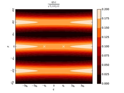
(a) $|{\psi}\rangle=\frac{1}{N_{1}}(|{-q_{0},0}\rangle+|{q_{0},0}\rangle)$
In phase superposition of two coherent states along the x -axis.
$q_{0}$=0.4

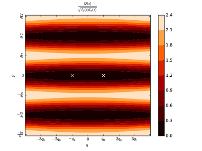
(b) $|{\psi}\rangle=\frac{1}{N_{2}}(|{-q_{0},0}\rangle-|{q_{0},0}\rangle)$
Out of phase superposition of two coherent states along the x -axis. $q_{0}$=0.4

Figure 2: Plot of $\frac{Q(z)}{\sqrt{I_{1}(z)I_{2}(z)}}$ in phase space for a superposition of two coherent states along the x-axis. We have divided the $Q$ distribution by $\sqrt{I_{1}(z)I_{2}(z)}$ to make the interference fringes more obvious. The positions of the coherent states are denoted by white crosses on the figure. Look at Eqn (56) for the relevant expressions.

That superposition of coherent states can lead to squeezing has been known for a while,Janszky and Vinogradov (1990) and has been interpreted Schleich et al. (1991); *Buzek1991; *Janszky_1993 using interference in phase space and the Wigner function of the superpositions. We will see later that this type of squeezing arising from in-phase superpositions becomes more dramatic as more and more coherent states are included. At the risk of repetition, we note that the purpose of the above exercise was to help the reader develop the following intuition, which will be borne out in the examples treated in the next Section.

• In-phase superposition of coherent states along a curve, tends to lead to the maximum of the $Q$ function lying on the curve.

• In-phase superposition along a curve leads to squeezing in the direction perpendicular to the curve.

• We saw in the above example that a shift in the relative phase between the two states in the superposition moves the fringes in a direction perpendicular to the line of superposition, without destroying the squeezing. In the continuum case, it continues to be expected that a phase gradient along the curve will shift the maximum in a direction perpendicular to the curve, maintaining the squeezing perpendicular to the curve.

III Phase space integral representations for position, momentum, and Fock states

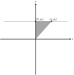
(a)  Orbit associated with $\hat{p}$

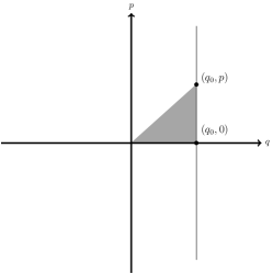
(b)   Orbit associated with $\hat{q}$

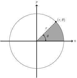
(c)  Orbit associated with $\hat{n}$

Figure 3: Phase plane orbits associated with the position, momentum and rotation generators in two dimensional phase space. The shaded areas (with appropriate signs) correspond to the phase factors which appear in the in-phase superpositions in Eqns. (65),(73),(82), as determined by Eqn. (46)

The position and momentum operators generate translations in phase space, while the number operator generates rotations. We will look at them in the sequence $\hat{p}$ (translations in $q$), $\hat{q}$ (translations in $p$), and the number operator $\hat{n}=\hat{a}^{\dagger}\hat{a}$ (rotations about the origin). These actions are associated with the corresponding orbits in the phase plane, leading to preferred in-phase integral representations for their eigenvectors. The first two will turn out to have global in-phase expansions, while for $\hat{n}$, we will obtain a local in-phase superposition.

III.1 Momentum eigenstates

The momentum operator $\hat{p}$ shifts the co-ordinate variable, leaving momentum unchanged:

$$e^{-iq^{\prime}\hat{p}} =D(q^{\prime},0),$$

$$D(q^{\prime},0)|{q,p_{0}}\rangle =e^{-\frac{i}{2}q^{\prime}p_{0}}|{q^{\prime}+q,p_{0}}\rangle.$$ (59)

Thus, the orbits in the phase plane associated with $\hat{p}$ action are, for each fixed $p_{0}$, the (horizontal) straight line $p_{0}\,=$ constant parallel to the $q$ axis. (Fig. 3(a))

Each such orbit, labelled by $p_{0}$, is a characteristic set. Therefore in principle, any $|{\psi}\rangle$ can be expanded in the form of a one-dimensional integral:

$$|{\psi}\rangle=\int_{-\infty}^{\infty}dq\,\,u(q)|{q,p_{0}}\rangle,\,\,p_{0}\,\,\text{fixed}.$$ (60)

Taking the overlaps with $\langle{q^{\prime},\text{pos}}|$ and $\langle{p^{\prime},\text{mom}}|$ leads to

$$\psi(q^{\prime}) =\frac{1}{{\pi}^{\frac{1}{4}}}\int_{-\infty}^{\infty}dq\,\,u(q)\exp[-\frac{1}{2}({q-q^{\prime}})^{2}+ip_{0}(q^{\prime}-\frac{q}{2})],$$

$$\tilde{\psi}(p^{\prime}) =\frac{1}{{\pi}^{\frac{1}{4}}}\exp[-\frac{1}{2}{(p_{0}-p^{\prime})}^{2}]\int_{-\infty}^{\infty}dq\,\,u(q)\exp[-iq(p^{\prime}-\frac{p_{0}}{2})].$$ (61)

The first relation is rather unwieldy, so we use the second. By Fourier inversion, we can express $u(q)$ in terms of $\tilde{\psi}(p^{\prime})$:

$$u(q)=\frac{1}{2\pi^{3/4}}e^{-\frac{i}{2}qp_{0}}\int_{-\infty}^{\infty}dp^{\prime}\,\,\tilde{\psi}(p^{\prime})e^{\frac{1}{2}{(p^{\prime}-p_{0})}^{2}+ip^{\prime}q}\leavevmode\nobreak\ \leavevmode\nobreak\ .$$ (62)

In general, for a square integrable $\tilde{\psi}(p^{\prime})$, $u(q)$ is a distribution. For any fixed $p_{0}$, as $u(q)$ is unambiguously determined by $|{\psi}\rangle$, the one–dimensional family of coherent states $\{|{q,p_{0}}\rangle,-\infty<q<\infty\}$ is linearly independent, and the expansion in Eqn. (60) is unique.

For the momentum eigenstate,

$$|{\psi}\rangle =|{p^{\prime}_{0},\text{mom}}\rangle,\quad\tilde{\psi}(p^{\prime})=\delta(p^{\prime}-p^{\prime}_{0}):$$

$$u(q) =\frac{1}{2\pi^{3/4}}\,\exp[\frac{1}{2}{(p_{0}-p^{\prime}_{0})}^{2}+iq(p^{\prime}_{0}-\frac{p_{0}}{2})],$$

$$|{p^{\prime}_{0},\text{mom}}\rangle =\frac{1}{2\pi^{3/4}}\,\exp[\frac{1}{2}{(p_{0}-p^{\prime}_{0})}^{2}]\int_{-\infty}^{\infty}dq\exp[iq(p^{\prime}_{0}-\frac{p_{0}}{2})]|{q,p_{0}}\rangle.$$ (63)

If we examine the integrand here, we find that in general these vectors are out of phase :

$$\phi_{P}\left(\exp[iq^{\prime}(p^{\prime}_{0}-\frac{1}{2}p_{0})]\,\,|{q^{\prime},p_{0}}\rangle,\exp[iq(p^{\prime}_{0}-\frac{1}{2}p_{0})]\,\,|{q,p_{0}}\rangle\right)=-(q^{\prime}-q)(p^{\prime}_{0}-p_{0}).$$ (64)

For given $|{p^{\prime}_{0},\text{mom}}\rangle$, the preferred expansion via such integrals is obtained when $p_{0}=p^{\prime}_{0}$, so that it becomes an in-phase superposition:

$$|{p^{\prime}_{0},\text{mom}}\rangle=\frac{1}{2\pi^{3/4}}\int_{-\infty}^{\infty}dq\exp[\frac{i}{2}qp^{\prime}_{0}]\,\,|{q,p^{\prime}_{0}}\rangle.$$ (65)

Now that we have constructed the in-phase superposition, we note the following points

1. In Eqn. (III.1), the momentum eigenstate $|{p^{\prime}_{0},\text{mom}}\rangle$ is concentrated along $p^{\prime}_{0}$, while the superposition which results in it is along the line $p_{0}$ in phase space. Splitting the phase factor $\exp[iq(p^{\prime}_{0}-\frac{p_{0}}{2})]$ as $\exp[iqp_{0}/2]\exp[iq(p^{\prime}_{0}-{p_{0}})]$, we see that in the absence of the phase gradient $\exp[iq(p^{\prime}_{0}-{p_{0}})]$, the R.H.S. of Eqn. (III.1), would have been an in-phase superposition and the result would have stayed put at the location $p_{0}$. The phase gradient drives the superposition precisely by the amount $p^{\prime}_{0}-p_{0}$ to $p^{\prime}_{0}$. Since the amplitude of the coherent states on $p_{0}$ is small on $p^{\prime}_{0}$ by the factor $\exp\left[-\frac{1}{2}(p_{0}-p^{\prime}_{0})^{2}\right]$, we need the extra compensatory factor of $\exp\left[\frac{1}{2}(p_{0}-p^{\prime}_{0})^{2}\right]$on the R.H.S. in Eqn. (III.1). Hence, the superposition of $|{p^{\prime}_{0},\text{mom}}\rangle$ along any other line $p_{0}\neq p^{\prime}_{0}$ is inefficient.

2. Since we have an integral along a straight line, any three points on it form a degenerate triangle with vanishing area, so this is a globally in-phase superposition of coherent states. We stress that while $p^{\prime}_{0}$ and $p_{0}$ are independent in the valid expansion Eqn. (III.1), from the insights of geometric phase theory, we find the in-phase superposition Eqn. (65) a preferred one.

3. Note that a globally in-phase superposition along the straight line $p=p_{0}^{\prime}$ necessitates the phase $\frac{1}{2}qp^{\prime}_{0}$ in Eqn. (65). This can be easily seen using Eqn. (51).

   $$\phi_{P}(|{0,p_{0}}\rangle,|{q,p^{\prime}_{0}}\rangle) =A(0,0;0,p^{\prime}_{0};q,p^{\prime}_{0})=\frac{qp^{\prime}_{0}}{2}$$ (66)

4. A momentum eigenstate is one in which the momentum is infinitely squeezed. We saw in Section II that in-phase superposition of two coherent states $|{\pm q_{0},0}\rangle$ on the $q$ axis leads to some squeezing in $\hat{p}$, as seen in Eqn. (II.4), with maximum squeezing when $\theta=0$. Standing in between these two cases, Eqn. (II.4) with $\theta=0$ and Eqn. (65) is this example involving a globally in phase superposition, but with Gaussian weight. Apart from overall normalization,

   $$|{\psi}\rangle =\int_{-\infty}^{\infty}dq\exp[-\frac{\sigma^{2}q^{2}}{2}+\frac{i}{2}qp_{0}]\,|{q,p_{0}}\rangle,$$

   $${\tilde{\psi}(p)} =\langle{p,\text{mom}}|{\psi}\rangle=\sqrt{2}\frac{{\pi}^{\frac{1}{4}}}{\sigma}\exp[-\frac{1}{2}{(p-p_{0})}^{2}(1+\frac{1}{\sigma^{2}})].$$ (67)

   This shows a variable degree of squeezing in momentum, gradually tending to a momentum eigenstate(infinite squeezing) as $\sigma\rightarrow 0$.

5. Also note that while a phase gradient shifts the superposition, it does not affect the squeezing, as anticipated in the last paragraph in subsection II.4.

We can in principle seek an expansion of the form of Eqn. (60) even for a position eigenstate; using Eqn. (62),

$$|{\psi}\rangle =|{q^{\prime},\text{pos}}\rangle:\tilde{\psi}(p^{\prime})=\sqrt{\frac{1}{2\pi}}\exp[-iq^{\prime}p^{\prime}],$$

$$u(q) =\frac{1}{2{\pi}^{3/4}}\frac{1}{\sqrt{2\pi}}\exp[-\frac{i}{2}q\,p_{0}]\int_{-\infty}^{\infty}dp^{\prime}\exp[\frac{1}{2}{(p^{\prime}-p_{0})}^{2}+ip^{\prime}(q-q^{\prime})].$$ (68)

However, this is a quite badly behaved distribution, hence better avoided.

III.2 Position eigenstates

The position operator $\hat{q}$ shifts the momentum leaving position unchanged:

$$e^{ip^{\prime}\hat{q}}=D(0,p^{\prime}),$$

$$D(0,p^{\prime})|{q_{0},p}\rangle =e^{\frac{i}{2}p^{\prime}q_{0}}|{q_{0},p^{\prime}+p}\rangle.$$ (69)

Now, the phase plane orbits are, for each fixed $q_{0}$, a vertical straight line parallel to the $p$ axis. (Fig. 3(b))   Each such orbit is again a characteristic set, so in place of Eqns. (60), (III.1), we have:

$$|{\psi}\rangle =\int_{-\infty}^{\infty}dp\,\,v(p)|{q_{0},p}\rangle,$$

$$\psi(q^{\prime}) =\frac{1}{{\pi}^{\frac{1}{4}}}\exp[-\frac{1}{2}({q_{0}-q^{\prime}})^{2}]\int_{-\infty}^{\infty}dp\,\,v(p)\exp[ip(q^{\prime}-\frac{q_{0}}{2})],$$

$$\tilde{\psi}(p^{\prime}) =\frac{1}{{\pi}^{\frac{1}{4}}}\int_{-\infty}^{\infty}dp\,\,v(p)\exp[-\frac{1}{2}({p-p^{\prime}})^{2}-iq_{0}(p^{\prime}-\frac{p}{2})].$$ (70)

This time the first relation is easier to handle and gives:

$$v(p)=\frac{1}{2{\pi}^{3/4}}e^{\frac{i}{2}\,\,q_{0}p}\int_{-\infty}^{\infty}dq^{\prime}\,\,\psi(q^{\prime})\exp[\frac{1}{2}(q^{\prime}-q_{0})^{2}-iq^{\prime}p].$$ (71)

We draw conclusions similar in spirit to those from Eqn. (62): For a general square integrable $\psi(q^{\prime})$, $v(p)$ is a distribution. Given any fixed $q_{0}$, as $v(p)$ is unambiguously given by $\psi(q^{\prime})$, the one dimensional family of coherent states $\{|{q_{0},p}\rangle,-\infty<p<\infty\}$ is linearly independent and the expansion in Eqn. (III.2) is unique.

For a general position eigenstate, we find :

$$|{\psi}\rangle =|{q_{0}^{{}^{\prime}},\text{pos}}\rangle,\,\,{\psi}(q^{\prime})=\delta(q^{\prime}-q^{\prime}_{0});$$

$$v(p) =\frac{1}{2\pi^{3/4}}\exp[\frac{1}{2}{(q_{0}-q^{\prime}_{0})}^{2}-ip(q^{\prime}_{0}-\frac{q_{0}}{2})],$$

$$|{q^{\prime}_{0},\text{pos}}\rangle =\frac{1}{2\pi^{3/4}}\exp[\frac{1}{2}{(q_{0}-q^{\prime}_{0})}^{2}]\int_{-\infty}^{\infty}dp\,\,\exp[-ip(q^{\prime}_{0}-\frac{q_{0}}{2})]\,\,|{q_{0},p}\rangle.$$ (72)

If $q_{0}\neq q^{\prime}_{0}$ this is not an in phase superposition. It becomes one (in fact globally so) if we choose $q_{0}=q^{\prime}_{0}$, and then we get the preferred expansion

$$|{q^{\prime}_{0},\text{pos}}\rangle=\frac{1}{{2\pi}^{\frac{3}{4}}}\int_{-\infty}^{\infty}dp\,\,e^{-i\frac{q^{\prime}_{0}p}{2}}\,\,|{q^{\prime}_{0},p}\rangle.$$ (73)

As in the case of momentum eigenstates, we see that the phase $\exp[-ip(q^{\prime}_{0}-\frac{q_{0}}{2})]$ in Eqn. (III.2) can be split up into

$$\exp[-ip(q^{\prime}_{0}-{q_{0}})]\exp[-ipq_{0}/2]$$

But for the factor of $\exp[-ip(q^{\prime}_{0}-{q_{0}})]$, we would have obtained an in-phase superposition along $q_{0}$. This phase gradient along $q_{0}$ drives the superposition from $q_{0}$ to $q^{\prime}_{0}$. Also, the inefficient superposition of $|{q^{\prime}_{0},\text{pos}}\rangle$ along $q_{0}$ necessitates the exponentially large compensatory factor $\exp\left[\frac{1}{2}(q_{0}-q^{\prime}_{0})^{2}\right]$, to make up for the exponentially small overlap of coherent states at $q_{0}$ on $q_{0}^{\prime}$.

Again, the phase in Eqn. (73) for global in-phase superposition along the straight line $q=q_{0}$ can be determined by using Eqn. (51)

$$\phi_{P}(|{q_{0},0}\rangle,|{q_{0},p}\rangle) =A(0,0;q_{0},0;q_{0},p)=-\frac{q_{0}p}{2}$$

where the negative sign accounts for the fact that the vertices are traversed clockwise.

III.3 Fock states

The operator $\hat{n}=\hat{a}^{\dagger}\hat{a}$ generates rotations in phase space

$$e^{i\theta\hat{n}}|{z}\rangle =|{ze^{i\theta}}\rangle$$

$$e^{i\theta\hat{n}}|{q,p}\rangle =|{q\cos\theta-p\sin\theta,p\cos\theta+q\sin\theta}\rangle.$$ (74)

The associated orbits are circles (Fig. 3(c)) centred on $q=p=0$. In essence, this describes what is “coherent” about coherent states– under time evolution by the Hamiltonian

$$H =\hat{a}^{\dagger}\hat{a}+\frac{1}{2}$$

$$e^{-i\hat{H}t}|{z}\rangle =e^{-it/2}|{ze^{-i\theta}}\rangle$$ (75)

the coherent state remains an eigenstate of $\hat{a}$ while being rotated around the classical constant energy circle $\frac{1}{2}({q}^{2}+{p}^{2})$. This example is very different from the two previous ones since the orbit here is a closed curve.

Each such orbit is a characteristic set, so in principle any $|{\psi}\rangle$ can be expanded as an integral over a circle of coherent states for any fixed $r>0$. However, such a subset is not a linearly independent set (in contrast to what we found in the cases of $\hat{p}$ and $\hat{q}$), as

$$\int_{0}^{2\pi}d\theta\leavevmode\nobreak\ e^{im\theta}|{r\cos\theta,r\sin\theta}\rangle=0,\,\,m\,=\,1,2,3\cdots$$ (76)

These states are overcomplete. Therefore in expanding $|{\psi}\rangle$ as an integral over them we can limit the ‘expansion coefficients’ suitably :

$$|{\psi}\rangle=\int_{0}^{2\pi}d\theta\,v(\theta)|{r\cos\theta,r\sin\theta}\rangle,$$

$$v(\theta)=\sum_{m=0}^{\infty}v_{m}e^{-im\theta}.$$ (77)

(Note that in Eqn. (III.3) negative values of $m$ do not appear in the expansion for $v(\theta)$.)

Then $v(\theta),v_{m}$ are unique for given $|{\psi}\rangle$:

$$|{\psi}\rangle =\int_{0}^{2\pi}d\theta\sum_{m=0}^{\infty}v_{m}e^{-im\theta}\sum_{n=0}^{\infty}\frac{e^{-\frac{r^{2}}{4}}}{\sqrt{n!}}{\left(\frac{r}{\sqrt{2}}\right)}^{n}\,e^{in\theta}|{n}\rangle$$

$$=2\pi e^{-\frac{r^{2}}{4}}\sum_{n=0}^{\infty}\frac{v_{n}}{\sqrt{n!}}{\left(\frac{r}{\sqrt{2}}\right)}^{n}|{n}\rangle;$$

$$v_{n} =\frac{{e^{\frac{r^{2}}{4}}}}{2\pi}\sqrt{n!}{\left(\frac{\sqrt{2}}{r}\right)}^{n}\,\psi_{n},\quad\psi_{n}=\langle{n}|{\psi}\rangle.$$ (78)

The result is that while $\{\psi_{n}\}$ is always an $l^{2}$ sequence for normalisable $|{\psi}\rangle$, in general $\{v_{n}\}$ is not so. This makes $v(\theta)$ in general non-$L^{2}$, but a distribution. Formally, we have

$$v(\theta)=\frac{1}{2\pi}e^{\frac{r^{2}}{4}}\sum_{n=0}^{\infty}\sqrt{n!}{\left(\frac{\sqrt{2}}{r}\right)}^{n}e^{-in\theta}\psi_{n},$$ (79)

and in all of Eqns. (76) to (79), $r$ can be chosen and kept fixed at any value.

Now, we choose $|{\psi}\rangle$ to be a Fock state $|{n}\rangle$, an eigenstate of $\hat{n}$ with eigenvalue $n$. Then $v(\theta)$ is just a single term in the sum in Eqn. (79) and we have the integral representation (valid for any $r\,\,>$  0). This is well-known, see, for example Gardiner (1983).

$$|{n}\rangle=\frac{e^{\frac{r^{2}}{4}}}{2\pi}\sqrt{n!}{\left(\frac{\sqrt{2}}{r}\right)}^{n}\,\int_{0}^{2\pi}d\theta e^{-in\theta}|{r\cos\theta,r\sin\theta}\rangle.$$ (80)

In general this is not an in-phase superposition since

$$\phi_{P}\left(e^{-in\theta}|{r\cos\theta,r\sin\theta}\rangle,e^{-in(\theta+\delta\theta)}|{r\cos(\theta+\delta\theta),r\sin(\theta+\delta\theta)}\rangle\right)=\left(\frac{r^{2}}{2}-n\right)\delta\theta.$$ (81)

We get a locally in phase superposition if given $n$, we choose $r^{2}=2n$; then we obtain the preferred integral representation

$$|{n}\rangle=\frac{e^{n/2}}{2\pi}\sqrt{n!}n^{-n/2}\int_{0}^{2\pi}d\theta e^{-in\theta}|{\sqrt{2n}\cos\theta,\sqrt{2n}\sin\theta}\rangle$$ (82)

for Fock states. Since the integration is over a circle (not a straight line as in Eqns. (65), (73), any three distinct points on it enclose a non-degenerate triangle with non-zero area. Thus, in contrast with the previous two examples, we have here only a locally in-phase superposition, not a global one.

Also note that in Eqn. (80), we could have split the phase factor as in the momentum and position eigenstates as

$$e^{-in\theta}=e^{-i\frac{r^{2}\theta}{2}}e^{i(\frac{r^{2}}{2}-n)\theta}$$

But for the phase gradient of $\left(\frac{r^{2}}{2}-n\right)\theta$ along the circle, the superposition would have been in phase and stayed put at $r$. The phase gradient drives the superposition away from the circle at radius $r$ to radius $\sqrt{2n}$.

We point out that the preferred in-phase superpositions for the Fock states satisfy the condition

$$\oint pdq=2\pi n$$ (83)

This would be the Bohr-Sommerfeld quantization condition of “old” quantum theory! (the area is $2\pi n$ instead of $2\pi(n+\frac{1}{2})$.) Further, this is not a semiclassical result, it is exact.

We now return to the discussion around Eqn. (56), where we had made a case for curves of in-phase superpositions being the maxima of $Q$ functions. We now explicitly demonstrate that this is indeed the case for the three states considered.

The $Q$ distribution of the position, momentum and Fock states $|{q_{0},\text{pos}}\rangle$, $|{p_{0},\text{mom}}\rangle$ and $|{n}\rangle$ are

$$Q_{|{q_{0},\text{pos}}\rangle}(q,p) =\frac{1}{2\pi^{3/2}}\exp\left[-(q-q_{0})^{2}\right]$$

$$Q_{|{p_{0},\text{mom}}\rangle}(q,p) =\frac{1}{2\pi^{3/2}}\exp\left[-(p-p_{0})^{2}\right]$$

$$Q_{|{n}\rangle}(q,p) =\frac{1}{2\pi n!}\left[\frac{1}{2}(p^{2}+q^{2})\right]^{n}\exp\left[-\frac{1}{2}(p^{2}+q^{2})\right]$$ (84)

which, as can easily be verified, are maximized along the preferred curves corresponding to in-phase superpositions, i.e. $q=q_{0}$, $p=p_{0}$ and $p^{2}+q^{2}=2n$ respectively.

For the particular case of of the Fock state $n=5$ , we discretize the integral representation in Eqn. (80) as

$$|{n}\rangle=\frac{e^{\frac{r^{2}}{4}}}{2\pi}\sqrt{n!}{\left(\frac{\sqrt{2}}{r}\right)}^{n}\,\sum\limits_{j=0}^{N}e^{-i\frac{2\pi nj}{N}}|{\,r\cos\frac{2\pi j}{N},r\sin\frac{2\pi j}{N}\,}\rangle$$

and take $N=500$. In Figures  4(a), 4(b) we display the 500 states appearing in the sum on the RHS for two values of $r$ together with the $Q$ function for the Fock state $n=5$.

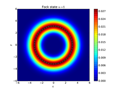
(a) (colour online) In-phase superposition along a circle of radius $\sqrt{2n}=\sqrt{10}$. Maximum of $Q$-function (black circles) located on the line of superposition. (white circles).

(b) (colour online) Superposition along a circle of radius $5$ (white circles). Maximum of Q-function is at $\sqrt{10}$, denoted by black circles

In Figure 4(a), the states are put on a circle of radius $\sqrt{2n}=\sqrt{10}$ (denoted by white dots) corresponding to their in-phase superposition. Note that in this case, the $Q$ function has a maximum (black circles) along the in-phase superposition. In contrast, as can be seen from Figure 4(b), this ceases to be so in the case when the states are put on a circle of radius $r=5$.

We conclude this section with a few clarifying comments. The overcompleteness of coherent states leads to enormous freedom in expanding a general vector $|{\psi}\rangle$ as an integral or sum over these states. With each of the generators $\hat{p},\hat{q},\hat{n}$, we are led in the first instance to consider one dimensional integral expansions for a general $|{\psi}\rangle$ over one of their associated orbits. For momentum eigenstates $|{p_{0},\text{mom}}\rangle$, in looking for an in-phase superposition we are led to a particular $\hat{p}$ orbit determined by $p_{0}$; similarly for the states $|{q_{0},\text{pos}}\rangle$ we are led to an in-phase integral over a corresponding $\hat{q}$ orbit determined by $q_{0}$; and lastly for Fock states $|{n}\rangle$ and corresponding $\hat{n}$ orbits, namely circles centred at the origin. The preferred eigenstate expansions in each case pick out a particular orbit of the concerned generator.

More generally, any locally in-phase sum or integral expansion, for any vector $|{\psi}\rangle$, of the form

$$|{\psi}\rangle =|{\psi_{1}}\rangle+|{\psi_{2}}\rangle+\cdots\,\,+|{\psi_{j}}\rangle+\cdots,\quad\text{arg}\langle{\psi_{j}}|{\psi_{j+1}}\rangle=0,$$

$$|{\psi}\rangle =\int ds|{\psi(s)}\rangle,\quad\text{arg}\langle{\psi(s)}|{\psi(s+\delta s)}\rangle=0,$$ (85)

retains these properties under any unitary transformation $U$, as inner products are preserved. As an example, if we start with the in-phase expansion in Eqn. (73) for a position eigenstate

$$|{q,\text{pos}}\rangle=\frac{1}{2\pi^{\frac{3}{4}}}\int_{-\infty}^{\infty}dp\,\,e^{-i\frac{qp}{2}}|{q,p}\rangle,$$ (86)

and apply the harmonic oscillator time evolution operator, we get using $\hat{H}=\hat{a}^{\dagger}\hat{a}+\frac{1}{2}$ along with Eqn. (III.3):

$$e^{-i\hat{H}t}|{q,\text{pos}}\rangle=\frac{1}{2\pi^{\frac{3}{4}}}\int_{-\infty}^{\infty}dp\,e^{-i\frac{qp}{2}-i\frac{t}{2}}|{q\cos t+p\sin t,p\cos t-q\sin t}\rangle,$$ (87)

and it is guaranteed that the right hand side is an in-phase superposition of a line of coherent states obtained from the line in Eqn. (86) by a clockwise rotation of amount $t$. Similarly, starting from the in-phase integral representation Eqn. (82) for Fock state $|{n}\rangle$ and applying the unitary displacement operator $D(q,p)$ (using Eqn (II.1)  ), we get the guaranteed-to-be in-phase superposition:

$$D(q,p)|{n}\rangle=\frac{e^{n/2}}{2\pi}\sqrt{n!}n^{-n/2}\int_{0}^{2\pi}d\theta\,e^{-in\theta+i\sqrt{\frac{n}{2}}(p\cos\theta-q\sin\theta)}|{q+\sqrt{2n}\cos\theta,p+\sqrt{2n}\sin\theta}\rangle.$$ (88)

So the integration is over a circle of radius $\sqrt{2n}$ with center $(q,p)$. We will exploit Eqns. (87) and (88) in the next section.

IV SOME APPLICATIONS OF THE FORMALISM

In this section, we present some sample calculations of overlaps of chosen state vectors, and some nontrivial matrix elements of interesting unitary operators of relevance to quantum optics, to convey the important features and advantages of the coherent state and geometric phase based in-phase superpositions. We illustrate how the one-dimensional integral in-phase representations of the position, momentum and number eigenstates derived in the previous section can be used to understand oscillations in state overlaps and make contact with previous work on interference in phase space.

IV.1 Sample state vector overlaps and matrix elements

In this subsection, we consider four examples of increasing complexity, to see how the ideas laid out in a general context in the preceding sections apply to specific state overlaps and matrix elements.

We have seen that the maximum of the $Q$ distribution lies along in-phase superpositions of coherent states. Guided by the intuition that state overlap is dominated by regions where the maximum of the corresponding $Q$ functions intersect, in each of the cases considered below, we calculate the critical point of the integrand. We see that it matches the geometric intersection of the in-phase integral representations, as we would expect without any calculation. We determine the overlap by expanding the integral about the critical point.

The first two examples, overlap of position-momentum eigenstates and the propagator for the harmonic oscillator, involve a single critical point and Gaussian integrals, and we recover well known exact results as expected.

The subsequent examples: Schrödinger wavefunction of a Fock state, and matrix elements of displacement operator in the Fock basis involve two critical points. Here, we get interference between the two contributions, resulting in oscillations. We connect the oscillations to areas by obtaining asymptotic results from the exact integral representations in the semiclassical limit of large quantum numbers. We demonstrate explicitly that the leading order contributions to the oscillatory part of the overlap can be determined from geometry and the in-phase superpositions alone, without actually evaluating any integrals.

1. We start with position-momentum overlap. It serves to illustrate some of the basic ideas outlined above in a simple setting.

   Use of the integral representations Eqns. (65), (73) followed by Eqn. (10b) leads to

   $$\langle q,\text{pos}|p,\text{mom}\rangle= {1\over 4\pi^{3/2}}\int_{-\infty}^{\infty}\int_{-\infty}^{\infty}dq^{\prime}dp^{\prime}e^{{i\over 2}(q^{\prime}p+p^{\prime}q)}\langle q,p^{\prime}|q^{\prime},p\rangle$$

   $$= {1\over 4\pi^{3/2}}e^{-{1\over 4}(q^{2}+p^{2})+{i\over 2}qp}\int_{-\infty}^{\infty}\int_{-\infty}^{\infty}dq^{\prime}dp^{\prime}e^{-\chi(q^{\prime},p^{\prime};q,p)}\,,$$

   $$\chi(q^{\prime},p^{\prime};q,p)= {1\over 4}(q^{\prime 2}+p^{\prime 2})-{1\over 2}(q^{\prime}q+p^{\prime}p)+{i\over 2}(q^{\prime}p^{\prime}-q^{\prime}p-p^{\prime}q)\,.$$ (89)

   The conditions ${\partial\chi\over\partial q^{\prime}}={\partial\chi\over\partial p^{\prime}}=0$ solve to give one critical point: $q^{\prime}=q$, $p^{\prime}=p$. This is precisely the point at which the phase plane orbits involved in the in-phase integral representations for $|p,\text{mom}\rangle$ and $|q,\text{pos}\rangle$ intersect, as was to be expected.

   Expanding about the point of intersection, we can rewrite the integral as

   $$\langle q,\text{pos}|p,\text{mom}\rangle= \frac{e^{iqp}}{4\pi^{3/2}}\int_{-\infty}^{\infty}\int_{-\infty}^{\infty}dq^{\prime}dp^{\prime}\exp(-\frac{1}{4}\left[(q^{\prime}-q)^{2}+(p^{\prime}-p)^{2}-2i(q^{\prime}-q)(p-p^{\prime})\right])$$

   Shifting the origin to the critical point,

   $$\langle q,\text{pos}|p,\text{mom}\rangle= \frac{e^{iqp}}{4\pi^{3/2}}\int_{-\infty}^{\infty}\int_{-\infty}^{\infty}dq^{\prime}dp^{\prime}e^{-\frac{1}{4}\left[{q^{\prime}}^{2}+{p^{\prime}}^{2}+2iq^{\prime}p^{\prime}\right]}$$

   $$=\frac{e^{iqp}}{4\pi^{3/2}}\int_{-\infty}^{\infty}\int_{-\infty}^{\infty}dq^{\prime}dp^{\prime}\exp\left[-\frac{1}{2}\begin{pmatrix}q^{\prime}&p^{\prime}\end{pmatrix}\begin{pmatrix}\frac{1}{2}&\frac{i}{2}\\ \frac{i}{2}&\frac{1}{2}\end{pmatrix}\begin{pmatrix}q^{\prime}\\ p^{\prime}\end{pmatrix}\right]$$

   $$=\frac{e^{iqp}}{4\pi^{3/2}}\times\frac{2\pi}{\sqrt{1/2}}\qquad\det\begin{pmatrix}\frac{1}{2}&\frac{i}{2}\\ \frac{i}{2}&\frac{1}{2}\end{pmatrix}=1/2$$

   $$=\frac{e^{iqp}}{\sqrt{2\pi}}$$ (90)

   In this case, we get the exact result as we are dealing with a Gaussian integral. Also, note that the phase of the overlap is determined entirely by the critical point.

2. Next, we consider the propagator of the simple harmonic oscillator in the position basis.

   

   Figure 4: Geometrical interpretation of the inner product $\langle q_{2},\,\mbox{pos}|e^{-iHt}|q_{1},\,\mbox{pos}\rangle$. The initial state $|q_{1}\rangle$ is given by an in phase superposition along the vertical line $q=q_{1}$ by Eqn. (73). $e^{-iHt}|q_{1},\,\mbox{pos}\rangle$ is determined by the rotated line. The stationary point of the exponent in the integrand, Eqn. (92) has a geometrical interpretation as the point of intersection of the in-phase superposition corresponding to $|q_{2},\,\mbox{pos}\rangle$ and the rotated line corresponding to $e^{-iHt}|q_{1},\,\mbox{pos}\rangle$.

   The effect of oscillator time evolution on a position eigenvector is given in Eqn. (87). Combining this with Eqn. (73) and (10b), we have the following configuration space kernel

   $$\langle q_{2},\text{pos}|e^{-i\hat{H}t}|q_{1},\text{pos}\rangle= {e^{-it/2}\over 4\pi^{3/2}}\int_{-\infty}^{\infty}dp_{1}\int_{-\infty}^{\infty}dp_{2}\leavevmode\nobreak\ e^{{i\over 2}(q_{2}p_{2}-q_{1}p_{1})}\langle q_{2},p_{2}|q_{1}C+p_{1}S,p_{1}C-q_{1}S\rangle$$

   $$= {e^{-it/2}\over 4\pi^{3/2}}\int_{-\infty}^{\infty}dp_{1}\int_{-\infty}^{\infty}dp_{2}\,\,e^{-Z}\,,$$

   $$Z={1\over 4}(p_{1}^{2}+p_{2}^{2})-{1\over 2}p_{1}p_{2}e^{-it} +{i\over 2}\left[(q_{1}-q_{2}e^{-it})p_{1}-(q_{2}-q_{1}e^{-it})p_{2}\right]+\frac{1}{4}(q_{1}^{2}+q_{2}^{2})-\frac{1}{2}q_{1}q_{2}e^{-it}\,,$$

   $$C= \cos t\leavevmode\nobreak\ ,\leavevmode\nobreak\ \leavevmode\nobreak\ S=\sin t\,.$$ (91)

   Alternatively, remembering how $\hat{n}$ rotates the coherent state $|{q,p}\rangle$, Eqn. (III.3)

   $$e^{i\theta\hat{n}}|{q,p}\rangle=|{q\cos\theta-p\sin\theta,p\cos\theta+q\sin\theta}\rangle.$$

   This leads to Fig. 4. Some geometry shows that the point of intersection has the co-ordinates

   $$p_{1}^{0}=q_{2}\mbox{ cosec}(t)-q_{1}\mbox{cot}(t);\leavevmode\nobreak\ \leavevmode\nobreak\ \leavevmode\nobreak\ p_{2}^{0}=q_{2}\mbox{cot}(t)-q_{1}\mbox{ cosec}(t)$$ (92)

   where $p_{1}^{0}$ is measured along the unrotated $|{q_{1},\text{ pos}}\rangle$ superposition. (Fig. 4)

   Indeed, we see that the stationary point of $Z(p_{1},p_{2})$ which would contribute maximally to the inner product leads to the same critical point, thus validating the geometrical interpretation.

   $$\frac{\partial Z}{\partial p_{1}}\bigg{|}_{(p_{1}^{0},p_{2}^{0})}=\frac{p_{1}^{0}}{2}-\frac{p_{2}^{0}}{2}e^{-it}+\frac{i}{2}(q_{1}-e^{-it}q_{2})=0;\leavevmode\nobreak\ \leavevmode\nobreak\ \frac{\partial Z}{\partial p_{2}}=\left(\frac{\partial Z}{\partial p_{1}}\right)^{\ast}=0$$ (93)

   Solving the real and imaginary parts of Eqn. (93), we again get back the stationary point with coordinates given by Eqn. (92).

   Expanding $Z$ about the critical point we get

   $$Z(p_{1},p_{2})-Z(p_{1}^{0},p_{2}^{0}) =\frac{1}{4}\left[(p_{1}-p_{1}^{0})^{2}+(p_{2}-p_{2}^{0})^{2}-2\,(p_{1}-p_{1}^{0})(p_{2}-p_{2}^{0})e^{-it}\right]$$

   $$Z(p_{1}^{0},p_{2}^{0}) =-i\left[\frac{\left(q_{1}^{2}+q_{2}^{2}\right)\cos t-2q_{1}q_{2}}{2\sin t}\right]$$ (94)

   Thus, we get

   $$\langle q_{2},\text{pos}|e^{-i\hat{H}t}|q_{1},\text{pos}\rangle= {e^{-it/2}\over 4\pi^{3/2}}\exp\left[-Z(p_{1}^{0},p_{2}^{0})\right]\int_{-\infty}^{\infty}dp_{1}\int_{-\infty}^{\infty}dp_{2}$$

   $$\exp\left(-\frac{1}{4}\left[(p_{1}-p_{1}^{0})^{2}+(p_{2}-p_{2}^{0})^{2}-2\,(p_{1}-p_{1}^{0})(p_{2}-p_{2}^{0})e^{-it}\right]\right)$$

   Shifting the origin to the critical point,

   $$\langle q_{2},\text{pos}|e^{-i\hat{H}t}|q_{1},\text{pos}\rangle =\exp\left[i\frac{(q_{1}^{2}+q_{2}^{2})\cos t-2q_{1}q_{2}}{2\sin t}\right]{e^{-it/2}\over 4\pi^{3/2}}\times$$

   $$\int_{-\infty}^{\infty}dp_{1}\int_{-\infty}^{\infty}dp_{2} \,\,\exp\left(-\frac{1}{4}\left[p_{1}^{2}+p_{2}^{2}-2p_{1}p_{2}e^{-it}\right]\right)$$

   $$=(2\pi i\sin t)^{-1/2}\exp\left[i\frac{(q_{1}^{2}+q_{2}^{2})\cos t-2q_{1}q_{2}}{2\sin t}\right]$$ (95)

   The special advantages of using in-phase integral representations for position eigenvectors when expanded in terms of coherent states should be evident.

3. In this third case, we encounter the first example where we have more than one critical point, and we get interference between their contributions. For the Schrödinger wave function of a Fock state, use of Eqns. (73), (82) followed by (10b) gives

   $$\langle q_{0},\text{pos}|n\rangle= {\mathcal{N}_{n}\over 4\pi^{7/4}}\int_{-\infty}^{\infty}dp_{1}\leavevmode\nobreak\ e^{{i\over 2}q_{0}p_{1}}\int_{0}^{2\pi}d\theta\leavevmode\nobreak\ e^{-in\theta}\langle q_{0},p_{1}|\sqrt{2n}\,C,\,\sqrt{2n}\,S\rangle$$

   $$= {\mathcal{N}_{n}\over 4\pi^{7/4}}\int_{0}^{2\pi}d\theta\leavevmode\nobreak\ e^{-in\theta-{1\over 4}(q_{0}-\sqrt{2n}C)^{2}+{i\over 2}q_{0}\sqrt{2n}S}$$

   $$\times\int_{-\infty}^{\infty}dp_{1}\leavevmode\nobreak\ e^{-{1\over 4}(p_{1}-\sqrt{2n}S)^{2}+{i\over 2}(q_{0}-\sqrt{2n}C)p_{1}}\,,$$

   $$C= \cos\theta\,,S=\sin\theta\,,\,\mathcal{N}_{n}=e^{n/2}n^{-n/2}\sqrt{n!}$$ (96)

   Shifting $p_{1}$, carrying out the Gaussian integral, remembering $n\geq 0$ and simplification by scaling leads to

   $$\langle q_{0},\text{pos}|n\rangle= {\mathcal{N}_{n}\over 2\pi^{5/4}}\int_{0}^{2\pi}d\theta\leavevmode\nobreak\ e^{-in\theta}e^{-{1\over 2}(q_{0}-\sqrt{2n}C)^{2}+iq_{0}\sqrt{2n}S-inCS}$$

   $$= {\mathcal{N}_{n}\over 2\pi^{5/4}}e^{-{n\over 2}-{q_{0}^{2}\over 2}}\int_{0}^{2\pi}d\theta\leavevmode\nobreak\ e^{-in\theta}e^{q_{0}\sqrt{2n}e^{i\theta}-{n\over 2}e^{2i\theta}}$$ (97a)

   $$= {\mathcal{N}_{n}\over\pi^{1/4}}e^{-{n\over 2}-{q_{0}^{2}\over 2}}\left[\frac{1}{2\pi i}\oint d\xi\frac{e^{q_{0}\sqrt{2n}\xi-\frac{n}{2}\xi^{2}}}{\xi^{n+1}}\right];\quad\xi=e^{i\theta}$$ (97b)

   $$= {\mathcal{N}_{n}\over\pi^{1/4}}{e^{{-n\over 2}-{q_{0}^{2}\over 2}}\over n!}\left({\partial^{n}\over\partial\xi^{n}}e^{q_{0}\sqrt{2n}\xi-{n\over 2}\xi^{2}}\right)_{\xi=0}$$

   $$= {\mathcal{N}_{n}\over\pi^{1/4}}{e^{{-n\over 2}-{q_{0}^{2}\over 2}}\over n!}\left({n\over 2}\right)^{n/2}\left({\partial^{n}\over\partial\xi^{n}}e^{2q_{0}\xi-\xi^{2}}\right)_{\xi=0}$$

   $$= {\mathcal{N}_{n}\over\pi^{1/4}}{e^{{-n\over 2}-{q_{0}^{2}\over 2}}\over n!}\left({n\over 2}\right)^{n/2}H_{n}(q_{0})\left(\mbox{using }\quad e^{2xt-t^{2}}=\sum_{n=0}^{\infty}H_{n}(x)\frac{t^{n}}{n!}\right)$$

   $$= {1\over\pi^{1/4}2^{n/2}\sqrt{n!}}\leavevmode\nobreak\ e^{-{q_{0}^{2}\over 2}}H_{n}(q_{0})$$ (97c)

   where $H_{n}(q_{0})$ are the Hermite polynomials. Again this example is meant only to illustrate the present formalism, yet it appears to be a shade more substantial than the previous one.

   Now, we use the in-phase integral representations of the Fock and the position eigenstates to give a geometric interpretation to the inner product $\langle q_{0},\text{pos}|n\rangle$ and simultaneously derive an asymptotic formula for the Hermite polynomials valid in the limit of large $n$.

   We start with Eqn. (97b). Analyticity of the integrand allows us to use the steepest descent formula. (accessible introductions can be found in Bleistein and Handelsman (1986); *krzywicki1996mathematics) We approximate

   $$I =\frac{1}{i}\oint d\xi\frac{e^{q_{0}\sqrt{2n}\xi-\frac{n}{2}\xi^{2}}}{\xi^{n+1}}$$

   $$=\frac{1}{i}\oint d\xi\frac{e^{nf(\xi)}}{\xi};\qquad f(\xi)=2C\xi-\frac{\xi^{2}}{2}-\log(\xi);\,q_{0}=\sqrt{2n}C$$

   In the limit of large $n$, the integral is dominated by contributions from the saddle point

   $$f^{\prime}(\xi_{0})=0; \quad\implies\xi_{0}=C\pm\sqrt{C^{2}-1}$$

   We are interested in the regime where the orbits of $|{n}\rangle$ and $|{q_{0},\text{pos}}\rangle$ intersect (at the two saddle points), and we get oscillatory behaviour due to interference from their contributions. Hence, we take $|C|<1$ and parametrize it as $C=\cos\theta_{0}$.

   Thus, the two saddle points are

   $$\xi_{0} =e^{\pm i\theta_{0}}$$ (98)

   Both these points satisfy $q_{0}=\sqrt{2n}\cos(\theta_{0})$, as expected from the intersection of the orbits in Fig.  5. $\pm\theta_{0}$ correspond to the points $P_{1}$ and $P_{2}$, respectively.

   

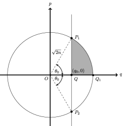
   Figure 5: The inner product $\langle q_{0},\text{pos}|n\rangle$ is determined in the steepest descent approximation by the two points $P_{1}$ and $P_{2}$ corresponding to the points of intersection of the in-phase superpositions of the Fock state $|n\rangle$ and the position eigenstate $|q_{0},\,\mbox{pos}\rangle$.

   In the neighbourhood of the critical points $\pm\theta_{0}$, $f^{\prime\prime}(e^{\pm i\theta_{0}})=\sin\theta_{0}\exp\left(\mp i(\theta_{0}+\frac{\pi}{2})\right)$.

   $$f(\xi)=f(\xi_{0})+r^{2}\sin(\theta_{0})e^{i\left[2\phi\mp(\frac{\pi}{2}+\theta)\right]};\quad\text{where }\,\xi-\xi_{0}=re^{i\phi};\quad\xi_{0}=e^{\pm i\theta_{0}}$$ (99)

   The direction of steepest descent $\phi$ in Eqn. (99) at the points $P_{1}$ and $P_{2}$ compatible with an anticlockwise contour turn out to be

   $$\phi{(\theta_{0})}=\frac{3\pi}{4}+\frac{\theta_{0}}{2};\qquad\phi{(-\theta_{0})}=\frac{\pi}{4}-\frac{\theta_{0}}{2}$$

   These are the directions along which the imaginary part stays constant and the real part decays. This allows us to extract the phase contribution from the critical point before integrating the Gaussian fluctuations. Adding up the contributions,

   $$I \approx\frac{e^{i(\frac{3\pi}{4}+\frac{\theta_{0}}{2})}}{ie^{i\theta_{0}}}\left[\int^{\infty}_{-\infty}dre^{-nr^{2}\sin\theta_{0}}\right]e^{nf(e^{i\theta_{0}})}+\frac{e^{i(\frac{\pi}{4}-\frac{\theta_{0}}{2})}}{ie^{-i\theta_{0}}}\left[\int^{\infty}_{-\infty}dre^{-nr^{2}\sin\theta_{0}}\right]e^{nf(e^{-i\theta_{0}})}$$

   $$e^{nf(e^{\pm i\theta_{0}})} =\exp\left[n\left(1+\frac{\cos 2\theta_{0}}{2}\right)\pm ni\left(\frac{\sin 2\theta_{0}}{2}-\theta_{0}\right)\right]$$

   After simplification,

   $$I \approx 2\sqrt{\frac{\pi}{n\sin\theta_{0}}}e^{n(1+\frac{\cos 2\theta_{0}}{2})}\cos\left[n\left(\frac{\sin 2\theta_{0}}{2}-\theta_{0}\right)+\frac{\pi}{4}-\frac{\theta_{0}}{2}\right]$$

   and hence

   $$\langle q_{0},\text{pos}|n\rangle\approx \frac{n^{-\frac{n}{2}}\sqrt{n!}}{\pi^{3/4}}\frac{e^{\frac{n}{2}}}{\sqrt{n\sin\theta_{0}}}\cos\left[\frac{\pi}{4}-\frac{\theta_{0}}{2}+n\left(\frac{\sin 2\theta_{0}}{2}-\theta_{0}\right)\right]$$

   $$\approx\left(\frac{2}{\pi^{2}n}\right)^{1/4}\frac{\cos\left[\frac{\pi}{4}-\frac{\theta_{0}}{2}+n\left(\frac{\sin 2\theta_{0}}{2}-\theta_{0}\right)\right]}{\sqrt{\sin\theta_{0}}}$$ (100)

   where in the last line we have used the Stirling approximation for $n!$.

   Now, note that the term proportional to $n$ in the argument of the cosine in Eqn. (100). is precisely half the area caught between the curves of in-phase superposition and is represented by the shaded portion in Fig.  5. It is

   $$\frac{1}{2}(\sqrt{2n})^{2}\theta_{0}-\frac{1}{2}(\sqrt{2n}\cos\theta_{0})(\sqrt{2n}\sin\theta_{0})=n\left(\theta_{0}-\frac{1}{2}\sin 2\theta_{0}\right)$$

   This is anticipated, considering the phase information in terms of areas was built into our integral representation through Eqn. (46). Phase associated with the Fock state at the point $P_{1}$ is $-n\theta_{0}$ = -Area ($P_{1}OQ_{1}$) subtended by the arc $P_{1}Q_{1}$ at the origin. Similarly, phase at $P_{1}$ for the position state is $-\frac{1}{2}q_{0}p(q_{0})=-\frac{n}{2}\sin(2\theta_{0})$. (the area of the triangle $P_{1}OQ$)

   So, the phase contribution to the inner product $\langle q_{0},\text{pos}|n\rangle$ is

   $$-\text{Area }(P_{1}OQ_{1})+\text{Area }(P_{1}OQ)=-\text{ Area }(P_{1}QQ_{1})$$

   which is precisely the negative of the shaded area.

   The extra term of $\frac{\pi}{4}$ in the argument of the cosine can be attributed to the turning point. The term $\frac{\theta_{0}}{2}$ comes with the factor of $\frac{\pi}{4}$ to enforce boundary conditions
   $H_{n}(q_{0}=0)\propto\cos\frac{n\pi}{2}$ (for $\theta_{0}=\frac{\pi}{2},\,q_{0}=0$.)

   Using the exact relation $\langle q_{0},\text{pos}|n\rangle={1\over\pi^{1/4}2^{n/2}\sqrt{n!}}\leavevmode\nobreak\ e^{-{q_{0}^{2}\over 2}}H_{n}(q_{0})$, we are led to an asymptotic expression of the Hermite polynomial

   $$e^{-\frac{q_{0}^{2}}{2}}H_{n}(q_{0}) \approx\left(2e\over n\right)^{\frac{n}{2}}\frac{n!}{\sqrt{\pi n\sin\theta_{0}}}\cos\left[\frac{\pi}{4}-\frac{\theta_{0}}{2}+n\left(\frac{\sin 2\theta_{0}}{2}-\theta_{0}\right)\right];\quad q_{0}=\sqrt{2n}\cos(\theta_{0})$$ (101)

   Using Stirling’s approximation for $n!$ we can simplify it to

   $$H_{n}(\sqrt{2n\cos\theta_{0}}) =\sqrt{\frac{2}{\sin\theta_{0}}}\left(2n\right)^{\frac{n}{2}}e^{\frac{n}{2}\cos 2\theta_{0}}\cos\left[\frac{\pi}{4}-\frac{\theta_{0}}{2}+n\left(\frac{\sin 2\theta_{0}}{2}-\theta_{0}\right)\right]$$ (102)

   Note that this expression is exactly the same as that obtained recently in Ref. Dominici (2007) through different techniques and was used for the estimation of zeros.

   

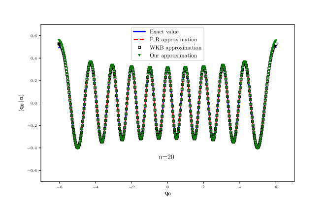
   Figure 6: Plot of $\langle q_{0}|n\rangle$ for n=20 using the exact value of the Hermite polynomial(solid blue line), Plancherel-Rotach approximation Eqn. (103) (dashed red line), WKB approximation Eqn. (104) (black squares) and our approximation Eqn. (100) (inverted green triangles). We interpolated between $q_{0}\in(-\sqrt{40}+0.3,\sqrt{40}-0.3)$ using 512 uniformly spaced points.

   We compare our results with the standard asymptotic expression due to Plancherel and Rotach Plancherel and Rotach (1929) ( referred to hereafter as the P-R approximation) available in the literature for $H_{n}(q_{0})$ as $n\rightarrow\infty$.

   $$e^{-\frac{q_{0}^{2}}{2}}H_{n}(q_{0}) \approx\frac{2^{n/2+1/4}\sqrt{n!}\left(\pi n\right)^{-\frac{1}{4}}}{\sqrt{\sin\theta}}\left\{\cos\left[\frac{\pi}{4}+(n+\frac{1}{2})\left(\frac{\sin 2\theta}{2}-\theta\right)\right]+O(n^{-1})\right\}$$ (103)

   $$q_{0} =\sqrt{2n+1}\cos\theta$$

   We also compare these with the WKB approximation, which yields

   $$\langle{q_{0},\text{ pos}}|n\rangle =\sqrt{\frac{2}{\pi\,p_{n}(q_{0})}}\cos\left(S_{n}(q_{0})-\frac{\pi}{4}\right)$$ (104)

   $$p_{n}(q_{0}) =\sqrt{2n+1-q_{0}^{2}}$$

   $$S_{n}(q_{0}) =(n+\frac{1}{2})\tan^{-1}\left(\frac{p_{n}(q_{0})}{q_{0}}\right)-\frac{1}{2}q_{0}p_{n}(q_{0})$$

   In Fig.  6, we display the plot for the exact $\langle q_{0},\text{pos}|n\rangle$ along with those corresponding to our asymptotic results, the P-R and WKB approximations. To the bare eye, all the approximations seem to be in good agreement with the exact result.

   $\,\,n\,\,$	RMSE (Our result)	RMSE(P-R)	RMSE (WKB)
   	Eqn. (100)	Eqn. (103)	Eqn. (104)
   20	0.0089	0.0053	0.0048
   30	0.0065	0.0041	0.0038
   40	0.0052	0.0035	0.0033
   50	0.0044	0.0030	0.0029

   Table 1: Root mean squared error for our, P-R and WKB approximation for ${1\over\pi^{1/4}2^{n/2}\sqrt{n!}}\leavevmode\nobreak\ e^{-{q_{0}^{2}\over 2}}H_{n}(q_{0})$ using $512$ equally spaced points for $q_{0}\in(-\sqrt{2n}+0.3,\sqrt{2n}-0.3)$ when compared with the exact result

   To probe the comparison between the three approximations further, we do a naive root mean squared error estimation from the exact value for a range of $n$ using $512$ equally spaced points between $(-\sqrt{2n}+0.3,\sqrt{2n}-0.3)$. These are summarised in Table 1.

   We see that the WKB approximation is better than the rest. Schleich Schleich (2001) has shown that the WKB approximation is equivalent to steepest descent such that the saddle points lie at a radial distance of $\sqrt{2n+1}$. Thus, it seems that for determining the values of Hermite polynomials, doing steepest descent over a contour of radius $\sqrt{2n+1}$ might be advantageous over $\sqrt{2n}$. As remarked before, Ref. Dominici (2007) obtains asymptotic expansions identical to ours for the purpose of estimating zeros of Hermite polynomials. Numerical approximations are not the subject of this paper, and we drop further investigations.

   We note here that all numerical results and plots presented in this section were generated with the mpmath library Johansson et al. (2013) with default precision, which translates to 15 decimal places.

4. The last case before moving on to squeezed states is the calculation of the Fock state matrix elements of the unitary displacement operator. In the now familiar fashion, using Eqns. (82), (88), (10b) and after simplification we have:

   $$\langle m|D(q,p)|n\rangle= {\mathcal{N}_{m}\mathcal{N}_{n}\over 4\pi^{2}}\int_{0}^{2\pi}d\theta\leavevmode\nobreak\ e^{im\theta}\int_{0}^{2\pi}d\theta^{\prime}\leavevmode\nobreak\ e^{-in\theta^{\prime}+i\sqrt{{n\over 2}}(pC^{\prime}-qS^{\prime})}$$

   $$\times\langle\sqrt{2m}C,\sqrt{2m}S|q+\sqrt{2n}C^{\prime},p+\sqrt{2n}S^{\prime}\rangle$$

   $$= {\mathcal{N}_{m}\mathcal{N}_{n}\over 4\pi^{2}}e^{-{1\over 2}(m+n)-{1\over 4}(q^{2}+p^{2})}\int_{0}^{2\pi}d\theta\leavevmode\nobreak\ e^{im\theta}\int_{0}^{2\pi}d\theta^{\prime}\leavevmode\nobreak\ e^{-in\theta^{\prime}}e^{Y}\,,$$

   $$Y= \sqrt{m}ze^{-i\theta}-\sqrt{n}z^{*}e^{i\theta^{\prime}}+\sqrt{mn}e^{i(\theta^{\prime}-\theta)},\,$$

   $$C= \cos\theta,\leavevmode\nobreak\ S=\sin\theta,\leavevmode\nobreak\ C^{\prime}=\cos\theta^{\prime},\leavevmode\nobreak\ S^{\prime}=\sin\theta^{\prime},\leavevmode\nobreak\ z={1\over\sqrt{2}}(q+ip)\,.$$ (105)

   Since $m,n\geq 0$ and $Y$ is a polynomial in $e^{-i\theta}$ and $e^{i\theta^{\prime}}$, putting $\xi=e^{-i\theta}$ and $\eta=e^{i\theta^{\prime}}$

   $$\langle m|D(q,p)|n\rangle={\mathcal{N}_{m}\mathcal{N}_{n}\over 4\pi^{2}}e^{-{1\over 2}(m+n)-{1\over 4}(q^{2}+p^{2})} \oint\limits_{\text{\tiny{clockwise}}}\frac{d\xi}{\xi^{m+1}}\oint\limits_{\text{\tiny{anticlockwise}}}\frac{d\eta}{\eta^{n+1}}e^{\sqrt{mn}\xi\eta+\sqrt{m}z\xi-\sqrt{n}z^{*}\eta}$$ (106a)

   $$={\mathcal{N}_{m}\mathcal{N}_{n}\over m!n!}e^{-{1\over 2}(m+n)-{1\over 4}(q^{2}+p^{2})} {\partial^{m}\over\partial\xi^{m}}{\partial^{n}\over\partial\eta^{n}}e^{\sqrt{mn}\xi\eta+\sqrt{m}z\xi-\sqrt{n}z^{*}\eta}|_{\xi=\eta=0}$$

   $$(\sqrt{m}\xi\rightarrow\xi,\,\sqrt{n}\eta\rightarrow\eta)\qquad ={e^{{1\over 4}(q^{2}+p^{2})}\over\sqrt{m!n!}}{\partial^{m}\over\partial\xi^{m}}{\partial^{n}\over\partial\eta^{n}}e^{(\eta+z)(\xi-z^{*})}|_{\xi=\eta=0}$$ (106b)

   $$={e^{{1\over 4}(q^{2}+p^{2})}\over\sqrt{m!n!}}{\partial^{m}\over\partial\xi^{m}}(\xi-z^{*})^{n}e^{z(\xi-z^{*})}|_{\xi=0}$$

   $$\left(\chi=z^{\ast}-\xi\right)\qquad ={e^{{1\over 4}(q^{2}+p^{2})}\over\sqrt{m!n!}}(-1)^{n-m}{\partial^{m}\over\partial\chi^{m}}(\chi^{n}e^{-z\chi})|_{\chi=z^{\ast}}$$

   $$z\chi\rightarrow\chi\qquad ={(-z)^{m-n}\over\sqrt{m!n!}}e^{{1\over 2}z^{*}z}\left({d^{m}\over d\chi^{m}}(e^{-\chi}\chi^{n})\right)_{\chi=z^{*}z}\,$$

   $$={\sqrt{m!}\over\sqrt{n!}}(-z^{*})^{n-m}e^{-{1\over 2}z^{*}z}L_{m}^{n-m}(z^{*}z)\,.$$ (106c)

   Alternatively, taking the $\xi$ derivative first in Eqn. (106b) yields

   $$\langle m|D(p,q)|n\rangle\, =\,\sqrt{\frac{n!}{m!}}z^{m-n}e^{-\frac{1}{2}z^{\ast}z}L_{n}^{m-n}\left(z^{\ast}z\right)$$ (107)

   The matrix element of the displacement operator in the Fock basis matches the form calculated in Cahill and Glauber (1969).

   We next use the in-phase integral representation in Eqn. $(\ref{a})$ for $\langle m|D(q,p)|n\rangle$ to obtain an asymptotic formula for $\langle m|D(q,p)|n\rangle$ valid in the limit of large $m,n$. This matrix element has been computed using phase space methods cited earlier Dowling et al. (1991),Mundarain and Stephany (2004).

   Since $\langle m|D(d\cos\phi,d\sin\phi)|n\rangle=e^{i\phi(m-n)}\langle m|D(d,0)|n\rangle$ it suffices to focus our attention on $\langle m|D(d,0)|n\rangle$, for which Eqn. (106a) yields:

   $$\langle m|D(d,0)|n\rangle=$$

   $$\frac{{\cal N}_{m}{\cal N}_{n}}{4\pi^{2}}e^{-{1\over 2}(m+n)-{1\over 4}d^{2}}\oint\limits_{\text{\tiny{clockwise}}}\frac{d\xi}{\xi^{m+1}}\oint\limits_{\text{\tiny{anticlockwise}}}\frac{d\eta}{\eta^{n+1}}e^{\sqrt{mn}\xi\eta+\sqrt{m}z\xi-\sqrt{n}z^{*}\eta}$$

   Rescaling, $\xi\rightarrow\sqrt{m}\xi$ and $\eta\rightarrow\sqrt{n}\eta$,

   $$\langle m|D(d,0)|n\rangle =C_{1}\oint\limits_{\text{\tiny{clockwise}}}d\xi\oint\limits_{\text{\tiny{anticlockwise}}}d\eta\frac{e^{f(\xi,\eta)}}{\xi\eta}$$ (108)

   $C_{1}=\frac{{\cal N}_{m}{\cal N}_{n}}{4\pi^{2}}m^{-\frac{m}{2}}n^{-\frac{n}{2}}e^{-{1\over 2}(m+n)-{1\over 4}d^{2}}$, $f(\xi,\eta)=mn\xi\eta+m\xi\frac{d}{\sqrt{2}}-n\eta\frac{d}{\sqrt{2}}-m\log(\xi)-n\log(\eta)$

   Henceforth, we will drop the clockwise and anticlockwise beneath the integrals. Now, the contours are defined as

   $$\xi=\frac{e^{-i\theta}}{\sqrt{m}};\quad \eta=\frac{e^{i\theta^{\prime}}}{\sqrt{n}}$$ (109)

   We take advantage of the analyticity of the integrand in ($\xi,\eta$) to calculate the matrix element in the semiclassical limit of large $m,n$ using the method of steepest descent. The saddle point of $f(\xi,\eta)$ yields

   $$\frac{\partial f(\xi,\eta)}{\partial\xi}\bigg{\rvert}_{\xi_{0}}=0. \qquad\mbox{ Solving, }\xi_{0}=\frac{1}{n\eta+\frac{d}{\sqrt{2}}},\qquad\frac{\partial^{2}f(\xi,\eta)}{\partial\xi^{2}}\bigg{\rvert}_{\xi_{0}}=\frac{m}{\xi_{0}^{2}}$$ (110)

   To integrate with respect to $\xi$, we expand $f(\xi,\eta)$ around the saddle point $\xi_{0}$ (which is now a function of $\eta$) and determine the direction of steepest descent

   $$f(\xi,\eta)-f(\xi_{0},\eta) =\frac{m}{2\xi_{0}^{2}}r^{2}e^{2i\phi}\qquad(\xi-\xi_{0}=re^{i\phi})$$

   Choice of $\phi$ compatible with a clockwise contour is $\phi=\mbox{arg}(\xi_{0})-\frac{\pi}{2}$. We calculate

   $$\langle{m}|D(d,0)|{n}\rangle =C_{1}\oint\frac{d\eta}{\xi_{0}\eta}e^{f(\xi_{0}(\eta),\eta)}\left(\int_{-\infty}^{\infty}dre^{-\frac{mr^{2}}{2|\xi_{0}|^{2}}}\right)(-i)e^{i\left[\text{{\small arg} }\xi_{0}\right]}$$

   $$=(-i)C_{1}\oint\frac{d\eta}{\xi_{0}\eta}e^{f(\xi_{0}(\eta),\eta)}\sqrt{\frac{2\pi}{m}}|\xi_{0}|e^{i\text{\small arg }(\xi_{0})}$$

   $$=(-i)C_{1}\sqrt{\frac{2\pi}{m}}\oint\frac{d\eta}{\eta}e^{f(\xi_{0}(\eta),\eta)}$$ (111)

   

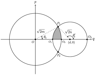
   Figure 7: Intersecting orbits of Fock state $m$ with another displaced Fock state $D(d,0)|n\rangle$

   Using Eqns. (110) and  (108), we get

   $$f(\xi_{0}(\eta),\eta) =m-n\eta\frac{d}{\sqrt{2}}+m\log\left(n\eta+\frac{d}{\sqrt{2}}\right)-n\log\eta$$ (112)

   Calculating the saddle point of $f(\xi_{0}(\eta),\eta)$ to compute the integral in $\eta$, we get

   $$\frac{\partial f(\xi_{0},\eta)}{\partial\eta}\bigg{\rvert}_{\eta_{0}}=0\,\,\implies\,\,\frac{1}{\eta_{0}}+\frac{d}{\sqrt{2}}=m\xi_{0}$$ (113)

   Putting the values from $\xi,\eta$ from Eqn. (109) in  (113) we get

   $$\sqrt{2m}e^{-i\theta_{0}}-\sqrt{2n}e^{-i\theta_{0}^{\prime}}=d \Leftrightarrow$$

   $$d=\sqrt{2m}\cos\theta_{0}-\sqrt{2n}\cos\theta_{0}^{\prime}\leavevmode\nobreak\ \leavevmode\nobreak\ ; \leavevmode\nobreak\ \leavevmode\nobreak\ \sqrt{2m}\sin\theta_{0}=\sqrt{2n}\sin\theta_{0}^{\prime}.$$ (114)

   Now, let us take a moment to appreciate this result in the light of Fig. 7. This is precisely the figure we would have drawn to depict the states $|{m}\rangle$ and $D(d,0)|{n}\rangle$, and would have been led to the same result as Eqn. (114). In other words, we could have anticipated the saddle point from geometry, guided by in-phase representations alone.

   As $\theta_{0},\theta^{\prime}_{0}$ are varied independently from $0$ to $2\pi$

   max. of $$|\sqrt{2m}e^{-i\theta_{0}}-\sqrt{2n}e^{-i\theta_{0}^{\prime}}|=\sqrt{2m}+\sqrt{2n},$$

   min. of $$|\sqrt{2m}e^{-i\theta_{0}}-\sqrt{2n}e^{-i\theta_{0}^{\prime}}|=|\sqrt{2m}-\sqrt{2n}|.$$

   Therefore, the necessary and sufficient conditions for existence of real solutions to the above conditions are

   $$|\sqrt{2m}-\sqrt{2n}|\leavevmode\nobreak\ \leq d\leavevmode\nobreak\ \leq\sqrt{2m}+\sqrt{2n}$$ (115)

   This is the regime we are going to be interested in. From Fig.  7, we can calculate the angles

   $$\theta_{0} =\cos^{-1}\left(\frac{d^{2}+2m-2n}{2\sqrt{2m}d}\right) \theta_{0}^{\prime}=\pi-\cos^{-1}\left(\frac{d^{2}+2n-2m}{2\sqrt{2n}d}\right)$$ (116)

   Using Eqns. (110), (113) in  (112) we get

   $$f(\xi_{0},\eta_{0}) =m+n-mn\xi_{0}\eta_{0}-m\log\xi_{0}-n\log\eta_{0}$$

   $$=m+n-\sqrt{mn}e^{\pm i(\theta_{0}^{\prime}-\theta_{0})}\pm i(m\theta_{0}-n\theta_{0}^{\prime})+\log(m^{\frac{m}{2}}n^{\frac{n}{2}})\text{ at }\pm(\theta_{0},\theta_{0}^{\prime})$$ (117)

   $$\frac{\partial^{2}f(\xi_{0},\eta)}{\partial\eta^{2}}\bigg{\rvert}_{\eta_{0}} =\frac{n}{\eta_{0}^{2}}-\frac{mn^{2}}{\left(n\eta_{0}+\frac{d}{\sqrt{2}}\right)^{2}}=\frac{n}{\eta_{0}^{2}}-\frac{mn^{2}}{\xi_{0}^{2}}$$

   Evaluating the value at the saddle points $\pm(\theta_{0},\theta_{0}^{\prime})$

   $$\frac{\partial^{2}f(\xi_{0},\eta)}{\partial\eta^{2}}\bigg{\rvert}_{\pm(\theta_{0},\theta_{0}^{\prime})} =2n^{2}\sin(\theta_{0}^{\prime}-\theta_{0})e^{\mp i\left(\theta_{0}+\theta_{0}^{\prime}+\frac{\pi}{2}\right)}$$ (118)

   We return to the integral

   $$\langle{m}|D(d,0)|{n}\rangle =(-i)C_{1}\sqrt{\frac{2\pi}{m}}\oint\frac{d\eta}{\eta}e^{f(\xi_{0},\eta)}$$

   $$\text{Let }I =\oint\frac{d\eta}{\eta}e^{f(\xi_{0},\eta)}$$

   In the neighbourhood of the critical points $\pm(\theta_{0},\theta_{0}^{\prime})$

   $$f(\xi_{0},\eta)-f(\xi_{0},\eta_{0})=r^{2}n^{2}\sin(\theta_{0}^{\prime}-\theta_{0})e^{i\left[2\phi\mp(\frac{\pi}{2}+\theta_{0}+\theta_{0}^{\prime})\right]};\quad\text{where }\,\xi-\xi_{0}=re^{i\phi};$$ (119)

   The directions of steepest descent at the points $\pm(\theta_{0},\theta_{0}^{\prime})$ compatible with a counterclockwise contour are $\frac{3\pi}{4}+\frac{\theta_{0}+\theta_{0}^{\prime}}{2}$ and $\frac{\pi}{4}-\frac{\theta_{0}+\theta_{0}^{\prime}}{2}$. Calculating the integral in $\eta$

   $$I =\int_{-\infty}^{\infty}dre^{-n^{2}r^{2}\sin(\theta_{0}^{\prime}-\theta_{0})}\left(\frac{e^{f(\xi_{0},\eta_{0})}}{\eta_{0}}\bigg{|}_{(\theta_{0},\theta_{0}^{\prime})}e^{i\left[\frac{3\pi}{4}+\frac{\theta_{0}+\theta_{0}^{\prime}}{2}\right]}+\frac{e^{f(\xi_{0},\eta_{0})}}{\eta_{0}}\bigg{|}_{(-\theta_{0},-\theta_{0}^{\prime})}e^{i\left[\frac{\pi}{4}-\frac{\theta_{0}+\theta_{0}^{\prime}}{2}\right]}\right)$$

   $$=\sqrt{\frac{\pi}{n\sin(\theta_{0}^{\prime}-\theta_{0})}}\left(e^{f(\xi_{0},\eta_{0})}\bigg{|}_{(\theta_{0},\theta_{0}^{\prime})}e^{i\left[\frac{3\pi}{4}+\frac{\theta_{0}-\theta_{0}^{\prime}}{2}\right]}-e^{f(\xi_{0},\eta_{0})}\bigg{|}_{(-\theta_{0},-\theta_{0}^{\prime})}e^{-i\left[\frac{3\pi}{4}+\frac{\theta_{0}-\theta_{0}^{\prime}}{2}\right]}\right)$$

   Using

   $$f(\xi_{0},\eta_{0})\bigg{|}_{(\theta_{0},\theta_{0}^{\prime})}=f(\xi_{0},\eta_{0})\bigg{|}_{(-\theta_{0},\theta_{0}^{\prime})}^{\ast}$$

   $$I =2i\sqrt{\frac{\pi}{n\sin(\theta_{0}^{\prime}-\theta_{0})}}\text{ Im}\left[e^{i\left(\frac{3\pi}{4}+\frac{\theta_{0}-\theta_{0}^{\prime}}{2}\right)}\times\exp{f(\xi_{0},\eta_{0})}\bigg{|}_{(\theta_{0},\theta_{0}^{\prime})}\right]$$

   $$=2i\,m^{\frac{m}{2}}n^{\frac{n}{2}}\sqrt{\frac{\pi}{n\sin(\theta_{0}^{\prime}-\theta_{0})}}\exp\left[m+n-\sqrt{mn}\cos(\theta_{0}^{\prime}-\theta_{0})\right]$$

   $$\times \sin\left[(m+\frac{1}{2})\theta_{0}-(n+\frac{1}{2})\theta_{0}^{\prime}+\frac{3\pi}{4}-\sqrt{mn}\sin(\theta^{\prime}_{0}-\theta_{0})\right]$$ (120)

   Using $\langle{m}|D(d,0)|{n}\rangle=(-i)C_{1}\sqrt{\frac{2\pi}{m}}I$, and simplifying, we get

   $$\langle m|D(d,0)|n\rangle \simeq\frac{n^{-\frac{n}{2}}m^{-\frac{m}{2}}}{\pi}\sqrt{\frac{m!n!}{2mn}}\,e^{n+m-\left[\frac{d^{2}}{4}+\sqrt{mn}\cos(\theta_{0}^{\prime}-\theta_{0})\right]}$$

   $$\times\dfrac{\cos[(m+{1\over 2})\theta_{0}-(n+{1\over 2})\theta_{0}^{\prime}+{\pi\over 4}-\sqrt{mn}\sin(\theta_{0}^{\prime}-\theta_{0})]}{\sqrt{\sin(\theta_{0}^{\prime}-\theta_{0})}}$$ (121)

   Use of Stirling’s formula ${\cal N}_{n}/{2\pi}\simeq(n/(2\pi)^{3})^{1/4}$ for large $n$ and likewise for ${\cal N}_{m}/{2\pi}$ for large $m$, we obtain:

   $$\langle m|D(d,0)|n\rangle \simeq\left(1\over{\pi^{2}mn}\right)^{1/4}e^{{1\over 2}(\sqrt{m}-\sqrt{n})^{2}-{d^{2}\over 4}}\times e^{\sqrt{mn}(1-\cos(\theta_{0}^{\prime}-\theta_{0}^{)})}$$

   $$\times\dfrac{\cos[(m+{1\over 2})\theta_{0}-(n+{1\over 2})\theta_{0}^{\prime}+{\pi\over 4}-\sqrt{mn}\sin(\theta_{0}^{\prime}-\theta_{0})]}{\sqrt{\sin(\theta_{0}^{\prime}-\theta_{0})}}.$$ (122)

   First, note that the leading order (in $m,n$) contributions to the oscillatory part of the overlap could have been obtained using the in-phase superpositions in Eqns. (82) and  (88) of $|{m}\rangle$ and $D(d,0)|{n}\rangle$ respectively, applied to the saddle point. Geometry determines the saddle point and hence leads to Eqn. (114). Thus, the contribution to the oscillatory phase due to the saddle points would be

   $$\text{Phase }D(d,0)|{n}\rangle-\text{ Phase }|{m}\rangle\,\bigg{|}_{P_{1}} =m\theta_{0}-n\theta_{0}^{\prime}-\sqrt{n}\sin\theta_{0}^{\prime}\frac{d}{\sqrt{2}}$$

   Using Eqn. (114) $$=m\theta_{0}-n\theta_{0}^{\prime}-\sqrt{mn}\sin(\theta_{0}^{\prime}-\theta_{0})$$

   which matches the leading order terms in the cosine, as expected. The phase at $P_{2}$ would just be negative of the term at $P_{1}$. The extra factors of $\frac{\pi}{4}$ can again be attributed to the turning point.

   Alternatively, we calculate the shaded area in Fig.  7

   $$n\pi+m\theta_{0}-n\theta_{0}^{\prime}+\frac{1}{2}(n\sin 2\theta_{0}^{\prime}-m\sin 2\theta_{0})$$

   $$= n\pi+m\theta_{0}-n\theta_{0}^{\prime}-\sqrt{mn}\sin(\theta_{0}^{\prime}-\theta_{0})$$ (123)

   The extra factor of $n\pi$ when we calculate areas, can be attributed to the fact that we determine the phase at the point $P_{1}$ for in-phase superpositions using the area swept out by the radius starting from $O_{3}$ to $P_{1}$, (with extra phase factors due to the action of $D(d,0)$) and not from $O_{1}$ to $P_{1}$. In fact, the in-phase superposition associates $0$ phase to $O_{3}$ and $-n\pi$ to $O_{1}$.

   For numerical comparison of the asymptotic expression for $\langle m|D(d,0)|n\rangle$ with the exact expression

   $$\langle m|D(d,0)|n\rangle={\sqrt{m!}\over\sqrt{n!}}\left(-{d\over{\sqrt{2}}}\right)^{n-m}e^{-{1\over 4}d^{2}}L_{m}^{n-m}\left({d^{2}\over{2}}\right)\,,$$ (124)

   we consider the cases $m=n$ and $m\neq n$ separately

   Case I) $m=n$

   In this case, the exact expression for $\langle m|D(d,0)|n\rangle$ becomes

   $$\langle m|D(d,0)|m\rangle=e^{-{1\over 4}d^{2}}L_{m}\left({d^{2}\over{2}}\right)\,.$$ (125)

   Further, Eqn. (116) for $\theta_{0}$ and $\theta_{0}^{\prime}$ in terms of $d$ and $m$ reduces to

   $$\theta_{0}=\cos^{-1}(d/2\sqrt{2m}),\quad\theta_{0}^{\prime}=\pi-\theta_{0}$$ (126)

   and the asymptotic expression for $\langle m|D(d,0)|m\rangle$ reads

   $$\langle m|D(d,0)|m\rangle \simeq\dfrac{m!}{\sqrt{2}\pi m^{m+1}}e^{2m+m\cos(2\theta_{0})-\frac{d^{2}}{4}}$$

   $$\times\dfrac{\cos[(2m+1)\theta_{0}-(m+{1\over 4})\pi-m\sin(2\theta_{0})]}{\sqrt{\sin(2\theta_{0})}}.$$ (127)

   Using Stirling’s approximation and simplifying:

   $$\langle m|D(d,0)|m\rangle \simeq\sqrt{\dfrac{1}{\pi m}}e^{-\frac{d^{2}}{4}+m(1+\cos(2\theta_{0}))}$$

   $$\times\dfrac{\cos[(2m+1)\theta_{0}-(m+{1\over 4})\pi-m\sin(2\theta_{0})]}{\sqrt{\sin(2\theta_{0})}}.$$ (128)

   Case II) $m\neq n$  

   In this case, we rewrite the Eqns. (116) and  (122) for convenience

   $$\theta_{0} =\cos^{-1}\left(\frac{d^{2}+2m-2n}{2\sqrt{2m}d}\right) \theta_{0}^{\prime}=\pi-\cos^{-1}\left(\frac{d^{2}+2n-2m}{2\sqrt{2n}d}\right)$$

   $$\langle m|D(d,0)|n\rangle \simeq\left(1\over{\pi^{2}mn}\right)^{1/4}e^{{1\over 2}(\sqrt{m}-\sqrt{n})^{2}-{d^{2}\over 4}}\times e^{\sqrt{mn}\left[1-\cos(\theta_{0}^{\prime}-\theta_{0})\right]}$$

   $$\times\dfrac{\cos[(m+{1\over 2})\theta_{0}-(n+{1\over 2})\theta_{0}^{\prime}+{\pi\over 4}-\sqrt{mn}\sin(\theta_{0}^{\prime}-\theta_{0})]}{\sqrt{\sin(\theta_{0}^{\prime}-\theta_{0})}}.$$

   It is instructive to compare our results for $\langle m|D(d,0)|n\rangle$ with those obtained using the asymptotic formulae for Laguerre polynomials due to Tricomi Tricomi (1949)

   $$e^{-\frac{1}{2}x}L_{n}^{\alpha}(x)=2(-1)^{n}(2\cos\theta)^{-\alpha}(\pi\nu\sin 2\theta)^{-1/2}\times$$

   $$\left(\sin\Theta+\frac{1}{12}\left(\frac{\nu\sin 2\theta}{4}\right)^{-1}\left[\frac{5}{4\sin^{2}\theta}-(1-3\alpha^{2})\sin^{2}\theta-1\right]\sin(\Theta+3\pi/2)+O(n^{-2})\right)$$

   $$\leavevmode\nobreak\ \leavevmode\nobreak\ \leavevmode\nobreak\ \leavevmode\nobreak\ \leavevmode\nobreak\ \leavevmode\nobreak\ \leavevmode\nobreak\ \leavevmode\nobreak\ \leavevmode\nobreak\ \leavevmode\nobreak\ \leavevmode\nobreak\ \leavevmode\nobreak\ x=\nu\cos^{2}\theta;\leavevmode\nobreak\ \leavevmode\nobreak\ \leavevmode\nobreak\ \nu=(4n+2\alpha+2)\qquad\Theta=\frac{\pi}{4}+\frac{\nu(2\theta-\sin(2\theta))}{4}$$ (129)

   valid in the ‘oscillatory region’ $0<x<\nu$ for large $n$. Using this formula in $(\ref{4.36})$ one obtains

   $$\langle m|D(d,0)|n\rangle\simeq(-1)^{n}\sqrt{\frac{m!}{n!}}\left(\frac{2}{\pi^{2}d^{2}}\right)^{1/4}\left(\frac{n+m+1}{2}\right)^{\frac{2n-2m-1}{4}}(\sin\theta)^{-1/2}$$

   $$\times\left(\sin\Theta+\frac{1}{12}\left(\frac{\nu\sin 2\theta}{4}\right)^{-1}\left[\frac{5}{4\sin^{2}\theta}-(1-3\alpha^{2})\sin^{2}\theta-1\right]\sin(\Theta+3\pi/2)\right)$$

   $$\nu=2(n+m+1);\alpha=n-m;\,\Theta=\frac{(n+m+1)}{2}(2\theta-\sin 2\theta)+\frac{\pi}{4};\,\,\theta=\cos^{-1}\left[\frac{d}{2\sqrt{n+m+1}}\right]$$ (130)

   As in the Hermite case, we also consider the WKB approximation (Dowling and Schleich Dowling et al. (1991)), who interpret their results in terms of interfering areas in phase space.

   $$\langle{m}|D(d,0)|{n}\rangle =2\sqrt{A_{m,n}}\cos(\phi_{m,n})$$ (131)

   $$A_{m,n}=\frac{1}{2\pi p_{m}(x_{c})}; \quad x_{c}=\frac{m-n}{d}+\frac{d}{2}$$

   $$p_{m}(x)=\sqrt{2m+1-x^{2}}; \quad\phi_{m,n}=S_{m,n}(x_{c})+\frac{\pi}{4}$$

   $$S_{m,n}=-\left(m+\frac{1}{2}\right)\sin^{-1}\left[\frac{x_{c}}{\sqrt{2m+1}}\right]+ \left(n+\frac{1}{2}\right)\sin^{-1}\left[\frac{x_{c}-d}{\sqrt{2n+1}}\right]-\frac{d}{2}\,\,p_{m}(x_{c})-(n-m)\frac{\pi}{2}$$

   

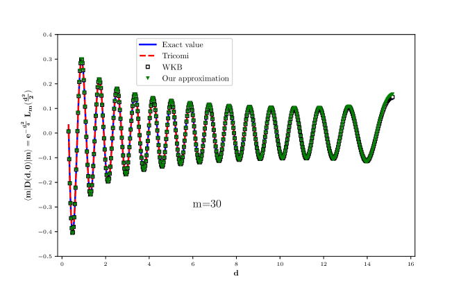
   Figure 8: Plot of $\langle{m}|D(d,0)|{m}\rangle$: Comparison of our approximation (128), Tricomi (130), and WKB (131) with the exact value.

   For $m=n=30$, Fig. 8 compares the exact results with the three approximations noted above. They match each other very well.

   For $m>n$ with $m=30$ and $n=20$, we compare our asymptotics with Tricomi in Fig. 9. Our approximation is visibly better than Tricomi’s. The performance of Tricomi’s approximation is particularly bad near the lower end at $d=\sqrt{2m}-\sqrt{2n}$. However, note that our results are similar to the WKB approximation in Fig. 10.

   

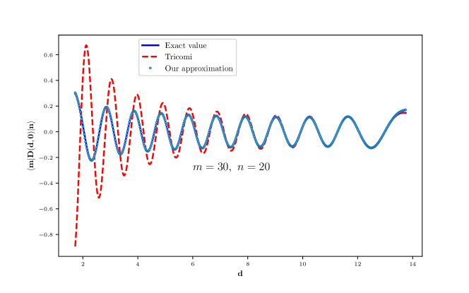
   Figure 9: Plot of $\langle{m}|D(d,0)|{n}\rangle$: Comparison of our approximation (122) and Tricomi (130)with the exact value.

   

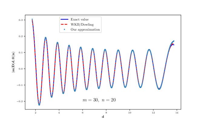
   Figure 10: Plot of $\langle{m}|D(d,0)|{n}\rangle$: Comparison of our approximation (122) and Dowling’s (131)with the exact value.

   To compare the closeness of the three approximations to the exact values we perform a simple root mean squared error analysis for $512$ equally spaced points in the range (a) $(\epsilon,2\sqrt{2m}+\epsilon)$ for the case when $m=n$ and (b) $(\sqrt{2m}-\sqrt{2n}+5,\sqrt{2m}+\sqrt{2n}-\epsilon)$ for the case when $m>n$ with $\epsilon=0.3$ as before. The results are summarised in the Tables 2 and 3.

   $\,\,m\,\,$	RMSE (Our result)	RMSE(Tricomi)	RMSE(WKB)
   	Eqn. (128)	Eqn. (130)	Eqn. (131)
   20	0.0048	0.0009	0.0036
   30	0.0032	0.0006	0.0025
   40	0.0023	0.0005	0.0018
   50	0.0018	0.0004	0.0013

   Table 2: Root mean squared error for our, Tricomi’s and the WKB approximation for
   $\langle{m}|D(d,0)|{m}\rangle$ using $512$ equally spaced points for $d\in(\epsilon,2\sqrt{2m}-\epsilon)$ when compared with the
   exact result. $\epsilon=0.3$ in the figure.

   $\,\,m\,\,$	$\,\,n\,\,$	RMSE (Our result)	RMSE(Tricomi)	RMSE (WKB)
   		Eqn. (122)	Eqn. (130)	Eqn. (131)
   30	20	0.0036	0.0143	0.0015
   40	30	0.0024	0.0099	0.0011
   50	40	0.0017	0.0076	0.0008
   30	10	0.0068	0.1198	0.0024

   Table 3: Root mean squared error for our, Tricomi’s and the WKB approximation for $\langle{m}|D(d,0)|{n}\rangle$ using $512$ equally spaced points for $d\in(\sqrt{2m}-\sqrt{2n}+\delta,\sqrt{2m}+\sqrt{2n}-\epsilon)$ when compared with the exact result. $\epsilon=0.3,\delta=5$ in the figure.We shift the lower limit asymmetrically so that Tricomi’s approximation does not produce large errors because of its poorer performance near the lower limit.

   This analysis shows that for $m=n$ Tricomi’s result works the best, for $m\neq n$, the WKB approximation fares better than the others. However, in each case, the approximations derived here have errors of the same order as the WKB method.

   As before, all the numerical results and plots in this section were generated with the mpmath library Johansson et al. (2013) with default precision. (15 decimal places)

IV.2 Selected squeezing operator matrix elements

In this subsection, we work with squeezed states. They are obtained by the action of the squeezing operator $S_{0}(\mu)$ on the vacuum state. We had remarked in the introduction that by the construction itself the generators of the $h_{4}$ algebra $\{\hat{q},\hat{p},\hat{a}^{\dagger}\hat{a}\}$ have simple actions on coherent states. In contrast, the squeezing operator has non-trivial action on coherent states. As a first step, we develop one dimensional in-phase integral representations in phase space for the squeezed vacuum. For any real $\mu$ let us define :

$$S_{0}(\mu) =e^{\frac{\mu}{4}\left[{(\hat{a}^{\dagger})}^{2}-\hat{a}^{2}\right]}$$ (132)

$$|\psi_{\mu}\rangle =S_{0}(\mu)|0\rangle\,.$$ (133)

The squeezing operator acts on the position and momentum operators as reciprocal scaling

$$S_{0}(\mu)(\hat{q},\hat{p})S_{0}(\mu)^{-1}= (e^{-\mu/2}\hat{q},\leavevmode\nobreak\ e^{\mu/2}\hat{p})\,,$$

$$S_{0}(\mu)D(q,p)S_{0}(\mu)^{-1}= D(e^{\mu/2}q,\leavevmode\nobreak\ e^{-\mu/2}p)\,,$$ (134)

From this the effects on position and momentum eigenstates follow:

$$S_{0}(\mu)|q,\text{pos}\rangle= e^{\mu/4}|e^{\mu/2}q,\text{pos}\rangle\,,$$

$$S_{0}(\mu)|p,\text{mom}\rangle= e^{-\mu/4}|e^{-\mu/2}p,\text{mom}\rangle\,.$$ (135)

As a result, for example, the Schrödinger wavefunction of a squeezed coherent state is, from Eqn. (II.1), read off immediately:

$$\langle q^{\prime},\text{pos}|S_{0}(\mu)|q,p\rangle={e^{-\mu/4}\over\pi^{1/4}}\exp\left\{-{1\over 2}(e^{-\mu/2}q^{\prime}-q)^{2}+ip(e^{-\mu/2}q^{\prime}-q/2)\right\}\,.$$ (136)

From Eqn. (136), the position and momentum space wavefunctions of the squeezed vacuum are:

$$\psi_{\mu}(q)={e^{-\mu/4}\over\pi^{1/4}}e^{-{1\over 2}e^{-\mu}q^{2}}\,,$$

$$\tilde{\psi}_{\mu}(p)={e^{\mu/4}\over\pi^{1/4}}e^{-{1\over 2}e^{\mu}p^{2}}\,.$$ (137)

Thus, consistent with Eqn. (135), for $\mu>0$ (respectively $\mu<0$), $|\psi_{\mu}\rangle$ is squeezed in momentum (respectively position). Therefore, we expect to obtain an integral representation along a horizontal line in the phase plane, as in Eqn. (60), if $\mu$ is positive; and along a vertical line as in Eqn. (III.2) if $\mu$ is negative. Indeed, following the steps given in Section III and using Eqns. (62), (71) in the two cases, we find the integral representations:

$$\mu>0,k= e^{\mu/2}:$$

$$|\psi_{\mu}\rangle= \sqrt{{k\over 2\pi(k^{2}-1)}}\,e^{k^{2}p^{2}_{0}/2(k^{2}-1)}\int_{-\infty}^{\infty}dq\leavevmode\nobreak\ e^{-q(q+i(k^{2}+1)p_{0})/2(k^{2}-1)}|q,p_{0}\rangle\,,\text{any}\leavevmode\nobreak\ p_{0}\,;$$ (138a)

$$\mu<0,k= e^{-\mu/2}:$$

$$|\psi_{\mu}\rangle= \sqrt{{k\over 2\pi(k^{2}-1)}}\,e^{k^{2}q^{2}_{0}/2(k^{2}-1)}\int_{-\infty}^{\infty}dp\leavevmode\nobreak\ e^{-p(p-i(k^{2}+1)q_{0})/2(k^{2}-1)}|q_{0},p\rangle\,,\text{any}\leavevmode\nobreak\ q_{0}\,;$$ (138b)

For general choices of $q_{0},p_{0}$ these are not in-phase integrals. For instance, for $\mu>0$, calculating the Pancharatnam phase between adjoining elements in the superposition one obtains

$$\phi_{P}\left[e^{-i(k^{2}+1)p_{0}q\over 2(k^{2}-1)}|q,p_{0}\rangle,e^{-i(k^{2}+1)p_{0}q^{\prime}\over 2(k^{2}-1)}|q^{\prime},p_{0}\rangle\right]=p_{0}(q-q^{\prime})\frac{k^{2}}{k^{2}-1}$$ (139)

which vanishes only when $p_{0}=0$. Similarly for $\mu<0$ this happens when $q_{0}=0$.

So we have the simpler preferred in-phase integral representations:

$$\mu>0:\leavevmode\nobreak\ \leavevmode\nobreak\ |\psi_{\mu}\rangle= \sqrt{{k\over 2\pi(k^{2}-1)}}\,\int_{-\infty}^{\infty}dq\leavevmode\nobreak\ e^{-q^{2}/2(k^{2}-1)}|q,0\rangle\,,$$ (140a)

$$\Delta p= {1\over k\sqrt{2}}\leavevmode\nobreak\ <\leavevmode\nobreak\ {1\over\sqrt{2}}\,;$$ (140b)

$$\mu<0:\leavevmode\nobreak\ \leavevmode\nobreak\ |\psi_{\mu}\rangle= \sqrt{{k\over 2\pi(k^{2}-1)}}\,\int_{-\infty}^{\infty}dp\leavevmode\nobreak\ e^{-p^{2}/2(k^{2}-1)}|0,p\rangle\,,$$ (140c)

$$\Delta q= {1\over k\sqrt{2}}\leavevmode\nobreak\ <\leavevmode\nobreak\ {1\over\sqrt{2}}\,;$$ (140d)

for the squeezed vacuum, with $k=e^{|\mu|\over 2}>1$. We note that these representations were first derived by Agarwal and Simon in Agarwal and Simon (1992), though without any particular reference to the in-phase nature of the superpositions involved.

In the final two examples, we study the overlap between Fock states and the squeezed coherent states and the squeezed number states. These have been extensively studied in the literature Yuen (1976),Satyanarayana (1985); *kral1990displaced and we compare our results for the matrix elements with the ones reported there. A detailed history of earlier works on these overlaps and comprehensive references may be found in Nieto (1997). In particular, we note that both these matrix elements have also been calculated in Földesi et al. (1995); *Janskysqueezedcoherent using a one dimensional representation of a squeezed displaced number state on a circle in conjunction with a one dimensional representation of a squeezed coherent state as a gaussian-weighted continuous superposition along the real axis.

a) As noted earlier, oscillations in the photon number distributions in the squeezed coherent states was one of the problems in which the notion of ‘interference in phase space’ first arose Schleich and Wheeler (1987); *Schleich_1988foundations, Schleich et al. (1988b), Schleich (2001),Mundarain and Stephany (2004). As a first application of the above integral representations, we compute the overlap between a Fock state and a squeezed coherent state which is a “mixed matrix element” of $S_{0}(\mu)$:

$$\langle n|S_{0}(\mu)|q,p\rangle=\langle n|S_{0}(\mu)D(q,p)|0\rangle\,.$$ (141)

Using Eqn. (134), we can move the displacement operator to the left of the squeezing operator with a change in the parameters:

$$S_{0}(\mu)D(q,p)=D(e^{\mu/2}q,\leavevmode\nobreak\ e^{-\mu/2}p)S_{0}(\mu)\,,$$ (142)

therefore we may equally well deal with the expression involving $|\psi_{\mu}\rangle$:

$$\langle n|D(q,p)S_{0}(\mu)|0\rangle=\langle n|D(q,p)|\psi_{\mu}\rangle\,.$$ (143)

Let us assume $\mu>0$. Then using (the conjugate of) Eqn. (88), followed by Eqns. (140a) and  (10b) we get:

$$\langle n|D(q,p)|\psi_{\mu}\rangle= {\mathcal{N}_{n}\over 2\pi}\sqrt{{k\over 2\pi(k^{2}-1)}}\int_{-\infty}^{\infty}dq^{\prime}\int_{0}^{2\pi}d\theta\leavevmode\nobreak\ e^{in\theta+i\sqrt{n\over 2}(pC-qS)-{q^{\prime 2}\over 2(k^{2}-1)}}$$

$$\times\langle\sqrt{2n}C-q,\sqrt{2n}S-p|q^{\prime},0\rangle\,$$

$$= {\mathcal{N}_{n}\over 2\pi}\sqrt{{k\over 2\pi(k^{2}-1)}}e^{-{n\over 2}-{1\over 4}(q^{2}+p^{2})}\int_{-\infty}^{\infty}dq^{\prime}\int_{0}^{2\pi}d\theta\leavevmode\nobreak\ e^{in\theta}e^{W}\,,$$

$$W= \sqrt{{n\over 2}}(q+ip+q^{\prime})e^{-i\theta}-{q^{\prime}\over 2}(q-ip)-{q^{\prime 2}\over 4}{k^{2}+1\over k^{2}-1}\,$$

$$C= \cos\theta,\leavevmode\nobreak\ S=\sin\theta\,.$$ (144)

As $n\geq 0$, the angular integration is immediate and leads to

$$\langle n|D(q,p)|\psi_{\mu}\rangle= {1\over\sqrt{2^{n}n!}}\sqrt{{k\over 2\pi(k^{2}-1)}}e^{-{1\over 4}(q^{2}+p^{2})}$$

$$\times\int_{-\infty}^{\infty}dq^{\prime}(q^{\prime}+q+ip)^{n}e^{-{q^{\prime 2}\over 4}{k^{2}+1\over k^{2}-1}-{q^{\prime}\over 2}(q-ip)}\,.$$ (145)

After a (complex) translation and then scaling the integration variable, we obtain a standard integral whose value involves a Hermite polynomial, and after simplification the final result is:

$$\langle n|D(q,p)|\psi_{\mu}\rangle= {i^{n}\over\sqrt{2^{n}n!}}\sqrt{{2k\over k^{2}+1}}\left({k^{2}-1\over k^{2}+1}\right)^{n/2}$$

$$\times\exp(-(q-ip)(q+ik^{2}p)/2(k^{2}+1))H_{n}\left({k^{2}p-iq\over\sqrt{k^{4}-1}}\right)\,.$$

$$k= e^{\mu/2}\leavevmode\nobreak\ ,\leavevmode\nobreak\ \leavevmode\nobreak\ \mu>0\,.$$ (146)

This result matches up with the one found in Yuen (1976),Satyanarayana (1985); *kral1990displaced. The case $\mu<0$ can be treated in a similar manner, but we forego the details.
b)  As a last example of the application of our phase space methods, we consider thematrix elements of the squeezing operator $S_{0}(\mu)$ in the Fock basis. This has relevance to the oscillations in the photon number distribution in squeezed Fock states. Ref Kim et al. (1989) analyzes it using the phase space approach, and finds four interfering regions instead of two as in the case of the photon distributions of squeezed coherent states.

Assume again $\mu>0$. The result Eqn. (146) just obtained comes in handy. Using Eqn. (82) for the ket in the matrix element of interest, we have with $k=e^{\mu/2}$, $C=\cos\theta$ and $S=\sin\theta$ as usual:

$$\langle n|S_{0}(\mu)|m\rangle= {\mathcal{N}_{m}\over 2\pi}\int_{0}^{2\pi}d\theta\leavevmode\nobreak\ e^{-im\theta}\langle n|S_{0}(\mu)|\sqrt{2m}C,\leavevmode\nobreak\ \sqrt{2m}S\rangle$$

$$= {\mathcal{N}_{m}\over 2\pi}\int_{0}^{2\pi}d\theta\leavevmode\nobreak\ e^{-im\theta}\langle n|S_{0}(\mu)D(\sqrt{2m}C,\sqrt{2m}S)|0\rangle$$

$$= {\mathcal{N}_{m}\over 2\pi}\int_{0}^{2\pi}d\theta\leavevmode\nobreak\ e^{-im\theta}\langle n|D(\sqrt{2m}kC,{\sqrt{2m}\over k}S)|\psi_{\mu}\rangle.$$ (147)

Here, we used Eqn. (134) in moving $S_{0}(\mu)$ to the right of the displacement operator. The matrix element inside the integrand is just what we computed in Eqn. (146), with the choices $q=\sqrt{2m}kC$, $p=\sqrt{2m}S/k$. After simplification of this expression to expose the $\theta$ dependencies, we have:

$$\langle n|S_{0}(\mu)|m\rangle= {\mathcal{N}_{m}\over 2\pi}{i^{n}\over\sqrt{2^{n}n!}}\sqrt{{}2k\over k^{2}+1}\left({k^{2}-1\over k^{2}+1}\right)^{n/2}e^{-m/2}$$

$$\times\int_{0}^{2\pi}d\theta\leavevmode\nobreak\ e^{-im\theta}e^{-{m\over 2}{k^{2}-1\over k^{2}+1}e^{2i\theta}}H_{n}\left({-ik\sqrt{2m}\over\sqrt{k^{4}-1}}e^{i\theta}\right)\,.$$ (148)

Note that $\langle n|S_{0}(\mu)|m\rangle$ is non-zero only when $m,n$ are both even(odd). The fact that this must be so follows from the fact that $S_{0}(\mu)$ is invariant under parity, and the eigenstates of the simple harmonic oscillator $|{m}\rangle$ and $|{n}\rangle$ have even(odd) parity depending upon whether $m,n$ is even(odd).

Carrying out the $\theta$-integration and after simplification we have the result for $\mu>0$:

$$\langle n|S_{0}(\mu)|m\rangle= \sqrt{{2k\over k^{2}+1}}{i^{n}\over\sqrt{2^{n}n!}}\left({k^{2}-1\over k^{2}+1}\right)^{n/2}{1\over\sqrt{m^{m}m!}}$$

$$\times{d^{m}\over d\xi^{m}}\left(e^{-{m\over 2}{k^{2}-1\over k^{2}+1}\xi^{2}}H_{n}\left({-ik\sqrt{2m}\over\sqrt{k^{4}-1}}\xi\right)\right)_{\xi=0}\,$$

$$=\frac{i^{n-m}}{\sqrt{2^{n}2^{m}}\sqrt{m!n!}}\sqrt{\frac{2k}{k^{2}+1}}{\left(\frac{k^{2}-1}{k^{2}+1}\right)}^{\frac{n+m}{2}}\frac{\partial^{m}}{\partial\xi^{m}}\left[e^{\xi^{2}}H_{n}\left(\frac{2k}{k^{2}-1}\xi\right)\right]_{\xi=0}$$ (149)

Using $H_{n}(x)={\left(-1\right)}^{n}e^{x^{2}}\frac{d^{n}}{dx^{n}}e^{-x^{2}}$ we get

$$\left[\frac{d^{m-p}}{d\xi^{m-p}}\,\,e^{\xi^{2}}\right]_{\xi=0}=-H_{m-p}(0)$$ (150)

Also,

$$\frac{d^{p}}{d\xi^{p}}\left[H_{n}\left(\frac{2k}{k^{2}-1}\xi\right)\right]_{\xi=0}=\left(\frac{4k}{k^{2}-1}\right)^{p}\frac{n!}{(n-p)!}H_{n-p}(0)$$ (151)

Using Leibnitz rule, we get

$$\langle n|S_{0}(\mu)|m\rangle =-\frac{i^{n-m}}{\sqrt{2^{n}2^{m}}\sqrt{m!n!}}\sqrt{\frac{2k}{k^{2}+1}}{\left(\frac{k^{2}-1}{k^{2}+1}\right)}^{\frac{n+m}{2}}\times$$ (152)

$$\sum_{p=0}^{\text{min}(m,n)}{m\choose p}\left(\frac{4k}{k^{2}-1}\right)^{p}\frac{n!}{(n-p)!}H_{n-p}(0)\,\,H_{m-p}(0)$$ (153)

Since,

$$H_{2n}(0)={\left(-1\right)}^{n}\frac{(2n)!}{n!};\,\,H_{2n+1}(0)=0;$$ (154)

we see that $\langle n|S_{0}(\mu)|m\rangle\,\,\neq 0$ only when $m-p$ and $n-p$ are simultaneously even which is only possible when $m,n$ have the same parity as previously noted. Thus, if $m-n$ is even

$$\langle n|S_{0}(\mu)|m\rangle=-i^{n-m} \frac{\sqrt{m!n!}}{\sqrt{2^{n}2^{m}}}\sqrt{\frac{2k}{k^{2}+1}}{\left(\frac{k^{2}-1}{k^{2}+1}\right)}^{\frac{n+m}{2}}\,\,\,\sum_{p=0}^{\text{min}(m,n)}\left(\frac{4k}{k^{2}-1}\right)^{p}\frac{\left(-1\right)^{\frac{m+n}{2}-p}}{p!\left(\frac{n-p}{2}\right)!\left(\frac{m-p}{2}\right)!}$$ (155)

where $p$ has the same parity as $m$ (or $n$). If $m-n$ is odd, $\langle n|S_{0}(\mu)|m\rangle=0$. Our result matches with the formula given in Ref. Satyanarayana (1985); *kral1990displaced.

V Concluding remarks

It is well known that owing to the overcompleteness of coherent states, a general vector in the Hilbert space can be expressed as a sum or integral over these states in many different ways. The question that we pose and answer in this work is : Can one find a useful general strategy that permits one to select a ‘preferred’ expansion from this multitude of possibilities ? In this work, guided by ideas and insights gained from the geometric phase theory, we propose one such scheme, which consists in demanding that the expansion be locally in-phase in the sense explained in the text. A particularly appealing feature of this strategy is that the property of an expansion being locally in phase is preserved under unitary transformations. The usefulness of the scheme proposed here is demonstrated by deriving exact and asymptotic expressions for a selection of overlaps and matrix elements of physical interest. Area considerations emerge naturally in this setting, and we discuss consequences of such superpositions on the behaviour of $Q$ functions. In-phase superpositions are seen to have bearing on squeezing too. Although the scheme developed in this work is in the context of the ‘harmonic oscillator’ or the Schrödinger coherent states, we have no doubt that the notion of ‘in-phase’ expansions based on the geometric phase theory will find useful applications in the context of other coherent state systems as well.

References

- Wigner (1932) E. Wigner, Phys. Rev. 40, 749 (1932).
- Dirac (1933) P. Dirac, 3, 64 (1933), phys. Zeits. Sowjetunion.
- Feynman (1949) R. P. Feynman, Phys. Rev. 76, 769 (1949).
- Feynman and Hibbs (1965) R. P. Feynman and A. R. Hibbs, Quantum Mechanics and Path Integrals (McGraw-Hill Companies, 1965).
- Schwinger (1951) J. Schwinger, Phys. Rev. 82, 914 (1951).
- Wick et al. (1952) G. C. Wick, A. S. Wightman, and E. P. Wigner, Phys. Rev. 88, 101 (1952).
- Giulini (2009) D. Giulini, in Compendium of Quantum Physics (Springer Science & Business Media, 2009) pp. 771–779, (A more recent account).
- Bartlett et al. (2007) S. D. Bartlett, T. Rudolph, and R. W. Spekkens, Rev. Mod. Phys. 79, 555 (2007).
- Klauder and Skagerstam (1985) J. Klauder and B. Skagerstam, Coherent States (World Scientific, 1985).
- Perelomov (1972) A. Perelomov, Communications in Mathematical Physics 26, 222 (1972).
- Perelomov (1986) A. Perelomov, Generalized Coherent States and Their Applications (Springer Science & Business Media, 1986).
- Misra and Sudarshan (1977) B. Misra and E. C. G. Sudarshan, J. Math. Phys. 18, 756 (1977).
- Berry (1984) M. V. Berry, Proceedings of the Royal Society A: Mathematical, Physical and Engineering Sciences 392, 45 (1984).
- Wilczek and Shapere (1989) F. Wilczek and A. Shapere, Geometric Phases in Physics (World Scientific, 1989).
- Bohm et al. (2003) A. Bohm, A. Mostafazadeh, H. Koizumi, Q. Niu, and J. Zwanziger, The Geometric Phase in Quantum Systems (Springer Science & Business Media, 2003).
- Xiao et al. (2010) D. Xiao, M.-C. Chang, and Q. Niu, Rev. Mod. Phys. 82, 1959 (2010).
- Prange and Girvin (1990) R. E. Prange and S. M. Girvin, eds., The Quantum Hall Effect (Springer New York, 1990).
- Macdonald (1994) A. H. Macdonald, arXiv preprint cond-mat/9410047 (1994).
- Girvin (1999) S. M. Girvin, in Aspects topologiques de la physique en basse dimension. Topological aspects of low dimensional systems (Springer, 1999) pp. 53–175.
- Stern (2008) A. Stern, Annals of Physics 323, 204 (2008).
- Tong (2016) D. Tong, arXiv preprint arXiv:1606.06687 (2016).
- Hasan and Kane (2010) M. Z. Hasan and C. L. Kane, Rev. Mod. Phys. 82, 3045 (2010).
- Qi and Zhang (2011) X.-L. Qi and S.-C. Zhang, Rev. Mod. Phys. 83, 1057 (2011).
- Bernevig and Hughes (2013) B. A. Bernevig and T. L. Hughes, Topological insulators and topological superconductors (Princeton university press, 2013).
- Franz and Molenkamp (2013) M. Franz and L. Molenkamp, “Contemporary concepts of condensed matter science: Topological insulators, vol. 6,” (2013).
- Rao (2016) S. Rao, arXiv preprint arXiv:1603.02821 (2016).
- Burkov (2018) A. A. Burkov, Annual Review of Condensed Matter Physics 9, 359 (2018).
- Armitage et al. (2018) N. P. Armitage, E. J. Mele, and A. Vishwanath, Rev. Mod. Phys. 90, 015001 (2018).
- Einstein et al. (1935) A. Einstein, B. Podolsky, and N. Rosen, Phys. Rev. 47, 777 (1935).
- Amico et al. (2008) L. Amico, R. Fazio, A. Osterloh, and V. Vedral, Rev. Mod. Phys. 80, 517 (2008).
- Horodecki et al. (2009) R. Horodecki, P. Horodecki, M. Horodecki, and K. Horodecki, Rev. Mod. Phys. 81, 865 (2009).
- Weyl (1927) H. Weyl, Zeitschrift für Physik 46, 1 (1927).
- Weyl (1950) H. Weyl, The theory of groups and quantum mechanics (Courier Corporation, 1950).
- Moyal (1949) J. E. Moyal, in Mathematical Proceedings of the Cambridge Philosophical Society, Vol. 45 (Cambridge Univ Press, 1949) pp. 99–124.
- Chaturvedi et al. (2006) S. Chaturvedi, E. Ercolessi, G. Marmo, G. Morandi, N. Mukunda, and R. Simon, J. Phys. A: Math. Gen. 39, 1405 (2006).
- Chaturvedi et al. (2010) S. Chaturvedi, N. Mukunda, and R. Simon, Journal of Physics A: Mathematical and Theoretical 43, 075302 (2010).
- Simon (1983) B. Simon, Phys. Rev. Lett. 51, 2167 (1983).
- Aharonov and Anandan (1987) Y. Aharonov and J. Anandan, Phys. Rev. Lett. 58, 1593 (1987).
- Samuel and Bhandari (1988) J. Samuel and R. Bhandari, Phys. Rev. Lett. 60, 2339 (1988).
- Mukunda and Simon (1993a) N. Mukunda and R. Simon, Annals of Physics 228, 205 (1993a).
- Mukunda and Simon (1993b) N. Mukunda and R. Simon, Annals of Physics 228, 269 (1993b).
- Pancharatnam (1956) S. Pancharatnam, Proceedings of the Indian Academy of Sciences - Section A 44, 247–262 (1956).
- Bargmann (1964) V. Bargmann, Journal of Mathematical Physics 5, 862 (1964).
- Wigner (1959) E. Wigner, Group Theory (Academic Press, New York, 1959) pp. 233-236.
- Simon et al. (2008) R. Simon, N. Mukunda, S. Chaturvedi, and V. Srinivasan, Physics Letters A 372, 6847 (2008).
- Simon et al. (2014) R. Simon, N. Mukunda, S. Chaturvedi, V. Srinivasan, and J. Hamhalter, Physics Letters A 378, 2332 (2014).
- Bargmann (1961) V. Bargmann, Communications on pure and applied mathematics 14, 187 (1961).
- Wheeler (1985) J. A. Wheeler, Letters in Mathematical Physics 10, 201 (1985).
- Schleich and Wheeler (1987) W. Schleich and J. A. Wheeler, Nature 326, 574 (1987).
- Schleich et al. (1988a) W. Schleich, H. Walther, and J. A. Wheeler, Foundations of Physics 18, 953 (1988a).
- Schleich et al. (1988b) W. Schleich, D. F. Walls, and J. A. Wheeler, Phys. Rev. A 38, 1177 (1988b).
- Dowling et al. (1991) J. P. Dowling, W. P. Schleich, and J. A. Wheeler, Ann. Phys. 503, 423 (1991).
- Schleich (2001) W. P. Schleich, Quantum Optics in Phase Space (Wiley-Blackwell, 2001).
- Xue et al. (2017) Y. Xue, T. Li, K. Kasai, Y. Okada-Shudo, M. Watanabe, and Y. Zhang, Scientific Reports 7, 2291 (2017).
- Mehmet et al. (2010) M. Mehmet, H. Vahlbruch, N. Lastzka, K. Danzmann, and R. Schnabel, Phys. Rev. A 81, 013814 (2010).
- Dutta et al. (1993) B. Dutta, N. Mukunda, R. Simon, and A. Subramaniam, Journal of the Optical Society of America B 10, 253 (1993).
- D. Krähmer and Schleich (1994) K. D. Krähmer, E. Mayr and W. Schleich, in Current Trends in Optics, edited by J.C.Dainty (Academic Press, London, 1994) Chap. 3, pp. 37–50.
- Janszky and Vinogradov (1990) J. Janszky and A. V. Vinogradov, Phys. Rev. Lett. 64, 2771 (1990).
- Schleich et al. (1991) W. Schleich, M. Pernigo, and F. L. Kien, Phys. Rev. A 44, 2172 (1991).
- Bužek and Knight (1991) V. Bužek and P. Knight, Optics Communications 81, 331 (1991).
- Janszky et al. (1993) J. Janszky, P. Domokos, and P. Adam, Phys. Rev. A 48, 2213 (1993).
- Kim et al. (1989) M. S. Kim, F. A. M. de Oliveira, and P. L. Knight, Phys. Rev. A 40, 2494 (1989).
- Milburn (1989) G. J. Milburn, in Squeezed and Nonclassical Light (Springer Science Business Media, 1989) pp. 151–159.
- Mundarain and Stephany (2004) D. F. Mundarain and J. Stephany, Journal of Physics A: Mathematical and General 37, 3869 (2004).
- Dominici (2007) D. Dominici, Journal of Difference Equations and Applications 13, 1115 (2007).
- Wineland (2013) D. J. Wineland, Rev. Mod. Phys. 85, 1103 (2013).
- Ourjoumtsev et al. (2007) A. Ourjoumtsev, H. Jeong, R. Tualle-Brouri, and P. Grangier, Nature 448, 784 (2007).
- Furusawa (2014) A. Furusawa (AIP Publishing, 2014).
- Sanders (2012) B. C. Sanders, Journal of Physics A: Mathematical and Theoretical 45, 244002 (2012).
- Glancy and de Vasconcelos (2008) S. Glancy and H. M. de Vasconcelos, Journal of the Optical Society of America B 25, 712 (2008).
- Bargmann et al. (1971) V. Bargmann, P. Butera, L. Girardello, and J. R. Klauder, Reports on Mathematical Physics 2, 221 (1971).
- Mukunda and Sudarshan (1978) N. Mukunda and E. Sudarshan, Pramana 10, 227 (1978).
- Chaturvedi et al. (1987) S. Chaturvedi, M. Sriram, and V. Srinivasan, Journal of Physics A: Mathematical and General 20, L1071 (1987).
- Yong-de and Lei (1990) Z. Yong-de and M. Lei, Il Nuovo Cimento B (1971-1996) 105, 1343 (1990).
- Field and Anandan (2004) T. R. Field and J. S. Anandan, Journal of Geometry and Physics 50, 56 (2004).
- Gardiner (1983) C. W. Gardiner, Springer series in synergetics (Springer, Berlin, 1983) includes indexes (1983), see page 377.
- Bleistein and Handelsman (1986) N. Bleistein and R. A. Handelsman, Asymptotic Expansions of Integrals (Dover Publications, 1986).
- Dennery and Krzywicki (1996) P. Dennery and A. Krzywicki, Mathematics for physicists (Mineola NY: Dover Publications, 1996).
- Plancherel and Rotach (1929) M. Plancherel and W. Rotach, Commentarii Mathematici Helvetici 1, 227–254 (1929), also see Orthogonal polynomials, Gabor Szegö,1939, Page 201.
- Johansson et al. (2013) F. Johansson et al., mpmath: a Python library for arbitrary-precision floating-point arithmetic (version 0.18) (2013), http://mpmath.org/.
- Cahill and Glauber (1969) K. E. Cahill and R. J. Glauber, Phys. Rev. 177, 1857 (1969).
- Tricomi (1949) F. G. Tricomi, Annali di Matematica Pura ed Applicata 28, 263–289 (1949), see Also Higher Transcendental Functions, Vol II, H.Bateman and A. Erdélyi (McGraw-Hill, 1953).
- Agarwal and Simon (1992) G. Agarwal and R. Simon, Optics Communications 92, 105 (1992).
- Yuen (1976) H. P. Yuen, Phys. Rev. A 13, 2226 (1976).
- Satyanarayana (1985) M. V. Satyanarayana, Phys. Rev. D 32, 400 (1985).
- Král (1990) P. Král, Journal of Modern Optics 37, 889 (1990).
- Nieto (1997) M. M. Nieto, Physics Letters A 229, 135 (1997).
- Földesi et al. (1995) I. Földesi, P. Adam, and J. Janszky, Physics Letters A 204, 16 (1995).
- Adam et al. (1990) P. Adam, J. Janszky, and A. Vinogradov, Optics Communications 80, 155 (1990).