Hairy black holes, boson stars and non-minimal coupling to curvature invariants

Abstract

The Einstein-Klein-Gordon Lagrangian is supplemented by a non-minimal coupling of the scalar field to specific geometric invariants : the Gauss-Bonnet term and the Chern-Simons term. The non-minimal coupling is chosen as a general quadratic polynomial in the scalar field and allows – depending on the parameters – for large families of hairy black holes to exist. These solutions are characterized, namely, by the number of nodes of the scalar function. The fundamental family encompasses black holes whose scalar hairs appear spontaneously and solutions presenting shift-symmetric hairs. When supplemented by a an appropriate potential, the model possesses both hairy black holes and non-topological solitons : boson stars. These latter exist in the standard Einstein-Klein-Gordon equations; it is shown that the coupling to the Gauss-Bonnet term modifies considerably their domain of classical stability.

1 Introduction

Attempts to escape the rigidity of the minimal Einstein-Hilbert formulation of gravity and the limited number of parameters describing its fundamental solutions – the black holes –, lead naturally physicists to emphasize enlarged models of gravity. Besides their purely Academic interests, these attempts are largely motivated nowadays by intriguing problems such as inflation, dark matter and dark energy.

One of the most popular class of extensions of Einstein gravity consists in the inclusion of scalar fields and appeals for natural interactions between the scalar fields and the geometry through higher curvature terms, leaving a lot of freedom. The general construction of scalar-tensor gravity leading to second order field equations was first obtained in [1]. Recently this theory was revived in the context of Galileon theory [2] and different extensions of it, see e.g. [3].

Apart from their cosmological implications, the extended models of gravity (by scalar or other types of fields) offer possibilities to escape the limitations of the no-hair theorems [4, 5] holding in standard gravity. In the last few years, black holes endowed by scalar hairs have attracted a lot of attention and have been studied in numerous theories. One particularly interesting result is the family of hairy black holes constructed in [6] within the Einstein gravity minimally coupled to a complex scalar field. In this case, the no-hair theorems [4, 5] are bypassed by the rotation of the black hole and the synchronization of the spin of the black hole with the angular frequency of the scalar field. Recent reviews on the topic of black holes with scalar hairs can be found e.g. in [7],[8],[9].

The general theory of scalar-tensor gravity [1], [3] contains a lot of arbitrariness and the study of compact objects such as black holes, neutron stars or boson stars needs to be realized in some particular cases. As an example, the truncation of the Galileon theory to a lagrangian admitting a shift-symmetric scalar field was worked out by Sotiriou and Zhou (SZ in the following) [10] and still leads to a large family of models. Hairy black holes were constructed perturbatively and numerically in the particular case of a scalar field coupled linearly to the Gauss-Bonnet invariant [11].

Abandonning the hypothesis of shift-symmetry, several groups [12], [13], [14] considered during the past years, new types of coupling terms between a scalar field and specific geometric invariants (essentially the Gauss-Bonnet term). In these models the occurrence of hairy black holes results from an unstable mode of the scalar field equation in the background of a vacuum metric (the probe limit). The interacting term of the scalar field with the curvature invariant plays a role of potential and the coupling constant the role of a spectral parameter. By continuity, the hairy black holes then exist as solutions of the full system. It is used to say that the hairy black holes appear through a spontaneous scalarization for a sufficiently large value of the coupling constant.

In the present paper we will consider a model of scalar-tensor gravity encompassing the theories presenting a spontaneous scalarization and the shift-symmetry property. Families of classical solutions whose pattern extrapolates smoothly between shift-symmetric hairy black holes and spontaneous scalarized ones will be constructed . The type of structure found holds when coupling the scalar field to the Gauss-Bonnet invariant and to the Einstein-Chern-Simons invariant as well. All black holes solutions found are supported by the non-minimal coupling between the scalar field and the curvature invariant; however the field equations admit other types of solutions: boson stars. These regular solutions exist with a minimal coupling of scalar field to gravity but it will be shown that the non minimal coupling has important consequences on their stability properties.

The paper is organized as follow : in Sect. 2 we present the model to be studied. Namely the Einstein-Klein-Gordon Lagrangian extended by a non-minimal coupling. We discuss the spherically symmetric ansatz and the general form of the field equations. Sect. 3 is devoted to the presentation of the hairy black holes occurring in the model. The boson stars are presented in Sect. 4 with an emphasis on the influence of the non-minimal coupling of the spectrum of the solutions. Conclusions are drawn in Sect. 5. Similar results hold for Einstein-Chern-Simons gravity and are the object of the Appendix; the activation of the Chern-Simons term is realized by means of a NUT charge [15].

2 The model

2.1 The action

We are interested in solutions of the field equations associated with the action

$$S=\int\mathrm{d}^{4}x\sqrt{-g}\bigg{[}\frac{1}{16\pi\mathcal{G}}R-\nabla_{\mu}\phi^{*}\nabla^{\mu}\phi-V(\phi)+f(\phi){\cal I}(g)\bigg{]},$$ (2.1)

which extends the minimal Einstein-Klein-Gordon lagrangian. Here $R$ is the Ricci scalar and $\phi$ represents a complex scalar field which – in some circumstances – will be chosen real. The usual Klein-Gordon kinetic term is supplemented by a potential $V(\phi)$ which will actually be chosen as a function of the combination $|\phi|^{2}\equiv\phi\phi^{*}$ in order to ensure a $U(1)$ global symmetry for the scalar sector. In the following $V$ will be set in the form

$$V(\phi)=m^{2}|\phi|^{2}+\lambda_{4}|\phi|^{4}+\lambda_{6}|\phi|^{6}$$ (2.2)

which is used generically for obtaining Q-balls in the absence of gravity and boson stars when gravity is set in (see e.g. [16], [17] for reviews).

The gravity sector is supplemented by a non-minimal coupling between the scalar field and the geometrical invariant ${\cal I}(g)$. For this paper, we will be interested in the case where this invariant is the Gauss-Bonnet-scalar :

$${\cal I}(g)={\mathcal{L}}_{GB}\equiv R^{2}-4R_{ab}R^{ab}+R_{abcd}R^{abcd}.$$

It is well known that this invariant is a total derivative in four dimensions but it will contribute non trivially to the equations of motion through the non-minimal coupling to the scalar field via $f(\phi)$. For the seek of generality, we have also investigated the case of a coupling to the Chern-Simons invariant, see Appendix A.

In order to preserve the $U(1)$ symmetry of the “usual” scalar sector, we will assume that, just like the potential, $f(\phi)$ is a function of $|\phi|$. In this paper, we will emphasize the effects of a coupling function of the form

$$f(\phi)=\gamma_{1}|\phi|+\gamma_{2}|\phi|^{2}$$ (2.3)

where $\gamma_{1}$, $\gamma_{2}$ are independant coupling constants. Several forms of the function $f(\phi)$ have been emphasized in the literature where the scalar field is usually choosen real. The EGB theory with $\gamma_{2}=0$ and $V=0$ corresponds to a shift-symmetric theory studied by SZ [10], the case $\gamma_{1}=0$ is considered in [12], [13]. [14]. Several choices of the function $f(\phi)$ have been considered in [18] and very recently in [19],[20]. Solutions with the form of $f(\phi)$ above with two independant constants $\gamma_{1},\gamma_{2}$ was, to our knowledge, not yet investigated.

2.2 Equations of motion

The equations of motion (EOM) for the general action (2.1) read

$$G_{\mu\nu}=8\pi\mathcal{G}\left(T_{\mu\nu}^{(\phi)}+T_{\mu\nu}^{(\mathcal{I})}\right)$$ (2.4)

for the metric function, and

$$-\square\phi=-\frac{\partial V}{\partial\phi^{*}}+\frac{\partial f}{\partial\phi^{*}}\mathcal{I}(g)$$ (2.5)

for the scalar field. In these equations, $G_{\mu\nu}$ is the Einstein tensor and $\square=\nabla_{\mu}\nabla^{\mu}$. The energy momentum $T_{\mu\nu}^{(\phi)}$ arise from the variation of the standard Klein-Gordon lagrangian :

$$T_{\mu\nu}^{(\phi)}=\nabla_{\left(\mu\right.}\phi\nabla_{\left.\nu\right)}\phi^{*}-\left(\nabla_{\alpha}\phi^{*}\nabla^{\alpha}\phi+V(\phi)\right)g_{\mu\nu}\ \ .$$ (2.6)

Finally, $T_{\mu\nu}^{(\mathcal{I})}$ is the energy momentum tensor associated to the non-minimal coupling term $f(\phi)\mathcal{I}(g)$.

From Eq.(2.5), one can see that the invariant $\mathcal{I}(g)$ will act as a source term for the scalar field. Consequently, if one find a space-time solution of the EOM such that $\mathcal{I}(g)\neq 0$, this solution will automatically present a non-trivial scalar field. This mechanism is known as “curvature induced scalarization”.

2.3 The ansatz

2.3.1 Metric

We will be interested in spherically symmetric solutions. In this case, it is well known that (in the appropriate coordinate system) the metric can always be set in the form

$$\mathrm{d}s^{2}=-N(r)\sigma^{2}(r)\mathrm{d}t^{2}+\frac{1}{N(r)}\mathrm{d}r^{2}+g(r)(\mathrm{d}\theta^{2}+\sin^{2}\theta\mathrm{d}\varphi^{2})\ \ ,$$ (2.7)

where $\theta$ and $\varphi$ are the standard angles parameterising an $S^{2}$ with the usual range and $r$ and $t$ are the radial and time coordinates respectivelly.

The usual coordinate choice $g(r)=r^{2}$ will be used throughout this paper.

2.3.2 Scalar field

Within the same coordinate system, we choose a scalar field of the form

$$\phi(x^{\mu})=e^{-i\omega t}\phi(r),$$ (2.8)

where $\omega$, the frequency of the scalar field, is a real parameter and $\phi(r)$ a real function. The scalar field will be assumed to be real (i.e. $\omega=0$) in the case of hairy black holes.

This choice above is motivated by the construction of boson stars. Indeed, it is well known [16] that boson stars exist as solutions of the minimal Einstein-Klein-Gordon equations provided the scalar field is chosen complex (typically of the form (2.8)) and supplemented by a mass term (or a more general potential (2.2)) in the equations.

2.3.3 Reduced equations

With the Ansatz (2.7)–(2.8), the equations (2.4)–(2.5) reduces to a system of three coupled differential equations (plus a constraint) for the radial functions $N,\sigma$ and $\phi$. Using suitable combinations of the equations, the system is amenable to the form

$$N^{\prime}=F_{1}(N,\sigma,\phi,\phi^{\prime})\ \ ,\ \ \sigma^{\prime}=F_{2}(N,\sigma,\phi,\phi^{\prime})\ \ ,\ \ \phi^{\prime\prime}=F_{3}(N,\sigma,\phi,\phi^{\prime})$$ (2.9)

where $F_{a}$, with $a=1,2,3$, are involved algebraic expressions whose explicit form is not illuminating enough to be given.

2.3.4 Rescaling and units

In the coming discussion we will set $c=1$ and $8\pi G=1$. The equations are then invariant under the rescaling

$$r\rightarrow\lambda r\ \ \ ,m^{2}\rightarrow\frac{m^{2}}{\lambda^{2}}\ \ \ ,\ \ \ \lambda_{4,6}\rightarrow\frac{\lambda_{4,6}}{\lambda^{2}}\ \ \ \gamma_{1,2}\rightarrow\lambda^{2}\gamma_{1,2}\ ,$$ (2.10)

where $\lambda$ has the dimension of length^-1. These rescaled quantities will be used in the following. In the case of black holes we will use it to set the event horizon to unit (i.e. $r_{h}=1$). In the case of boson stars (which have no horizon) we will set the mass parameter $m$ to one ($m=1$).

3 Hairy black holes

3.1 Boundary conditions

We now discuss the black holes solutions of the equations. As stated above these solutions exist for a real scalar field, so we set $\omega=0$ in the equations. Let us first consider the solutions occuring in the absence of potential (i.e. setting $m=\lambda_{4}=\lambda_{6}=0$ in (2.2)); the influence of a mass term will be emphasized separately, see Sect. 3.2.3.

For black holes, the metric is required to present a regular horizon at $r=r_{h}$, i.e. $N(r_{h})=0$. The occurence of this condition in the equations and the requirement of a regular function $\phi(r)$ at the horizon implies a non trivial relation for the scalar function and its derivative at $r=r_{h}$. The two conditions at the horizon are summarized as follows

$$N(r_{h})=0\ \ \ ,\ \ \ \phi^{\prime}(r_{h})=\frac{-r_{h}^{2}\pm\sqrt{\Delta}}{8r_{h}(\gamma_{1}+2\gamma_{2}\phi(r_{h}))}\ \ ,\ \ \Delta=r_{h}^{4}-96\gamma_{1}^{2}-384(\gamma_{2}^{2}\phi(r_{h})^{2}+\gamma_{1}\gamma_{2}\phi(r_{h}))$$ (3.11)

Remark that $\Delta\geq 0$ constitutes a necessary condition for solutions to exist. We will see in the next section that it largely determines the domain of the coupling constants $\gamma_{1}$,$\gamma_{2}$ for which solutions exist. The requirement for the solutions to be asymtotically Minkowski further implies

$$\sigma(r\to\infty)=1\ \ \ \ ,\ \ \ \ \phi(r\to\infty)=0\ \ .$$ (3.12)

The four conditions (3.11)-(3.12) constitute the boundary values of the field equations. The black holes can be characterized by their mass $M$ and the scalar charge $Q_{s}$. These are related respectively to the asymptotic decay of the functions $N(r)$ and $\phi(r)$ :

$$N(r)=1-\frac{2M}{8\pi r}+O(1/r^{2})\ \ \ ,\ \ \ \phi(r)=\frac{Q_{s}}{r}+O(1/r^{2})\ \ .$$ (3.13)

The entropy $S=\pi r_{h}^{2}$ and temperature $T_{H}=\sigma(r_{h})N^{\prime}(r_{h})/(4\pi)$ characterize the solutions at the horizon. Using the equations the temperature can further be specified  :

$$N^{\prime}(r_{h})=\frac{1}{r_{h}+4\phi^{\prime}(r_{h})(\gamma_{1}+2\gamma_{2}\phi(r_{h}))}\ \ .$$ (3.14)

Because the equations do not admit closed form solutions, we solved the system by using the numerical routine COLSYS [22] which is well adapted for the problem at hand. It is based on a collocation method for boundary-value differential equations and on damped Newton-Raphson iterations. The equations are solved with a mesh of a few hundred points and relative errors of the order of $10^{-6}$. The values $M,Q_{S},S,T_{H}$ can be extracted with such an accuracy from the numerical datas.

3.2 Numerical results

3.2.1 Fundamental branch

We now present the pattern of solutions in the $\gamma_{1},\gamma_{2}$ parameter space. Practically, we start from the hairy black holes constructed in [10], i.e. the shift-symmetric theory, corresponding to $\gamma_{2}=0$. A pair of solutions exist for $\gamma_{1}\leq\sqrt{1/96}\approx 0.1021$ (with our convention of the non minimal coupling); characterized by the sign $\pm$ appearing in the condition (3.11). We will essentially focus on the family of solutions corresponding to the “+” sign which, in the limit $\gamma_{1}\to 0$, smoothly approach the Schwarschild solution. Solutions corresponding to the “–” sign can be constructed as well (see e.g. [23]), forming a second branch whith higher mass. This branch, however is difficult to construct numerically. Moreover no regular solution can be associated to the $\gamma_{1}\to 0$ limit for this branch since the value $\phi^{\prime}(r_{h})$ in (3.11) clearly diverge in this case ($\gamma_{2}=0$) for the “$-$” sign. The understanding of this branch is then not aimed in the present paper.

For a fixed value of the parameter $\gamma_{1}$, the SZ solution can be deformed by increasing (or decreasing) gradually the coupling constant $\gamma_{2}$. The pattern of hairy black holes obtained in this way turns out to be quite different for the small values of $\gamma_{1}$ (say for $\gamma_{1}\leq 0.005$) and for $0.005<\gamma_{1}<\sqrt{1/96}$. For definiteness let us first discuss the family of black holes corresponding to $\gamma_{1}>0.005$.

1. Increasing gradually the coupling constant $\gamma_{2}$, it turns out that the value $\Delta$ approaches zero at some critical value, say $\gamma_{2,c}$. Accordingly, no solution exist for $\gamma_{2}>\gamma_{2,c}$. This is illustrated on Fig. 1 where the quantities $\Delta$ (solid lines) and $\phi(r_{h})$ (dashed lines) are plotted as functions of $\gamma_{2}$ for two values of $\gamma_{1}$ (see the purple and red lines). The corresponding values of the mass and of $\phi^{\prime}(r_{h})$ is presented on both sides of Fig. 2.

2. In the case $\gamma_{2}<0$, a Schwarzschild metric can be approached arbitrarily close, although not exactly. This is due to the fact that the scalar field never reaches $\phi(r)=0$ due to the presence of the non-homogeneous term in the scalar field equation. Indeed for the Schwarzschild black hole of mass $M$ we have ${\cal L}_{GB}=48M^{2}/r^{6}$.

The deformation of the SZ solutions in the region $\gamma_{1}\leq 0.005$ for $\gamma_{2}\neq 0$ leads to a richer pattern. For a fixed value of $\gamma_{1}\leq 0.005$ :

1. Starting from the shift-symmetric solution ($\gamma_{2}=0$) and increasing $\gamma_{2}>0$, we find that the SZ black holes forms a “first branch” of solutions which exists up to a maximal value, say for $\gamma_{2}\leq\gamma_{2,\max{}}$.

2. Then, decreasing $\gamma_{2}$ from $\gamma_{2,\max{}}$, a “second branch” of solutions exists for $\gamma_{2}\in[\gamma_{2,c},\gamma_{2,\max{}}]$. As before, the value $\gamma_{2,c}$ coincide with $\Delta=0$ and the two branches coincide in the limit $\gamma_{2}\to\gamma_{2,\max{}}$. Fig. 1 illustrates this phenomenon for $\gamma_{1}=0.0005$ (see the blue line; in this case we find $\gamma_{2,c}\approx 0.172$ and $\gamma_{2,\max{}}\approx 0.177$). We note that, on the interval of $\gamma_{2}$ where the two solutions coexist, the solution of the first branch has a lower mass than the corresponding solution on the second branch.

3. For $\gamma_{2}<0$, while decreasing $\gamma_{2}$, the black holes approach a Schwarzschild metric in the same way as point (ii) above.

To summarize, fixing low enough values of $\gamma_{1}$ and varying $\gamma_{2}>0$, the SZ solution deforms into a family of hairy black holes forming two branches which exist on specific intervals of $\gamma_{2}$. We can now emphasize how this ensemble behave when taking the limit $\gamma_{1}\to 0$. It turns out that the solutions of the first branch approach uniformly the Schwarzschild black hole (irrespectively of $\gamma_{2}$). By contrast, the solutions of the second branch have a non trivial limit and approach the set of so called “spontaneously scalarized black holes” for $\gamma_{2}\in[\gamma_{2,c},\gamma_{2,\max{}}]$. These solutions were constructed directly in [12],[13],[14]. The critical values $\gamma_{2,c}\approx 0.1734$ and $\gamma_{2,\max{}}\approx 0.1814$ found in these papers fit very well with our numerical datas. The occurence of these critical values have different explanations :

1. In the limit $\gamma_{2}\to\gamma_{2,c}$, the parameter $\Delta$ (see (3.11)) approaches zero.

2. In the limit $\gamma_{2}\to\gamma_{2,\max{}}$, the scalar hairs tends uniformly to zero.

The value $\gamma_{2,\max{}}$ in fact corresponds to an eigenvalue of the scalar field equation

$$\frac{1}{r^{2}}\frac{\mathrm{d}}{\mathrm{d}r}\left[r^{2}N(r)\frac{\mathrm{d}}{\mathrm{d}r}\phi\right]=\gamma_{2}\frac{48M}{r^{6}}\phi\ \ \ ,\ \ \ N(r)=1-\frac{2M}{r}$$ (3.15)

considered in the background of Schwarzschild solution. This value reflects a tachyonic instability of the Schwarzschild solution in the theory (2.1), opening the way for the vacuum solution to evolve into a hairy black hole. Details about the spectrum of this equation can be found, namely in [13], [21].

The question about the stability of our solutions raises naturally. In the case of the hairy black holes occuring by spontaneous scalarisation with a quadratic coupling to the Gauss-Bonnet term, it was shown in Refs. [19], [20] that the solutions present radial instabilities which can be removed when supplementing a quartic term in the coupling function. The study of the stability is not aimed in this paper; however we would like to argue about the (in)stability in the case where two solutions coexist with different masses on the interval $[\gamma_{2,c},\gamma_{2,\max{}}]$ (see Fig. 2). It is likely that the branch with the lower mass which approaches the Schwarzschild metric in the limit $\gamma_{1}\to 0$, is linearly stable while the branch with the higher mass, which approaches the spontaneously scalarized solutions, is unstable; this last statement being reinforced by a continuity argument applied to the results of [19], [20].

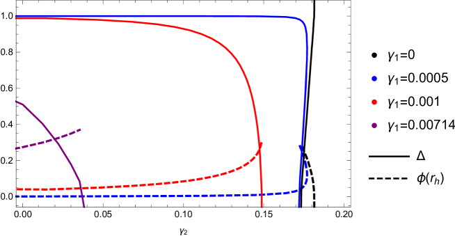
Figure 1: The parameter $\Delta$ (solid lines) and the value $\phi(r_{h})$ (dashed lines) as functions of $\gamma_{2}$ for several values of $\gamma_{1}$.

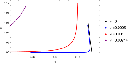
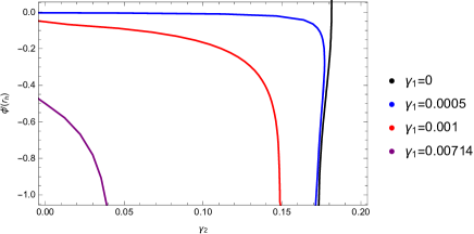
Figure 2: The mass as functions of $\gamma_{2}$ of the solutions of Fig.1. Right : Idem for the value $\phi^{\prime}(r_{h})$.

3.2.2 Excited solutions

In the shift-symmetric case, i.e. with $\gamma_{2}=0$, the condition (3.11) drastically reduces the spectrum of hairy black holes. For each value of $\gamma_{1}<1/\sqrt{96}$ a single solution is allowed whith “$+$” sign (since $\phi^{\prime}(r_{h})$ does not depend on $\phi(r_{h})$ but only on the fixed parameters $\gamma_{1}$ and $r_{h}$) and the scalar field is a monotonic function. Consequently, excited solutions (i.e. with $\phi(r)$ presenting nodes) do not occur. By contrast, for the spontaneously scalarized black holes (i.e. with $\gamma_{1}=0$), the linear equation (3.15) possesses – in principle – a series of critical values of $\gamma_{2}$ corresponding to normalizable eigenfunctions $\phi(r)$ presenting one or more nodes. Any of these solutions leads to a branch of excited hairy black holes of the coupled system ($\gamma_{1}\neq 0,\gamma_{2}\neq 0$). We constructed numerically the branch corresponding to the first excited (or one-node) solution. Values $\Delta$ and $\phi(x_{h})$ are reported on Fig. 3 as functions of $\gamma_{2}$ for a few values of $\gamma_{1}$ (the red lines correspond to $\gamma_{1}=0$). As for the fundamental (or no-node) solution discussed above, we see that the first excited hairy black holes exists for $\gamma_{2}\in[\gamma_{2,c},\gamma_{2,M}]$ where the lower (resp. upper) bound of this interval corresponds to $\Delta=0$ (resp. to the second eigenvalue of (3.15)).

Switching on the parameter $\gamma_{1}$ leads to a deformation of these excited hairy black holes. The results of Fig. 3 suggest that the excited black holes exist only for $\gamma_{2}\geq\gamma_{2,c}$. This contrasts drastically with the spectrum of fundamental solutions (see Fig.1). It is tempting to say that the fundamental solutions are “attracted” by the SZ solutions occurring in the $\gamma_{2}=0$ limit. Having no equivalent, the excited solutions exist only for large values of $\gamma_{2}$.

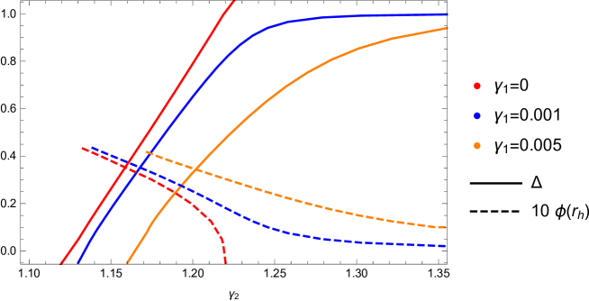
Figure 3: The value $\phi(r_{h})$ and the quantity $\Delta$ as function of $\gamma_{2}$ for several values of $\gamma_{1}$.

3.2.3 Influence of a mass term

In the previous section, the scalar field $\phi$ was supposed to be massless. In this section, we discuss the effect of a massive scalar field on the spectrum of hairy black holes. For simplicity we restrict the presentation to the spontaneously scalarized solutions – i.e. setting $\gamma_{1}=0$ – and to the mass term only in the potential (2.2) – i.e. $\lambda_{4}=\lambda_{6}=0$.

In the case of a massive scalar field, the regularity condition (3.11) is more involved :

$$\phi^{\prime}(r_{h})=\frac{-B\pm\sqrt{\Delta}}{2A}$$ (3.16)

with

$$A=-\phi_{0}(12\gamma_{2}-m^{2}r_{h}^{2}(r_{h}^{2}+8\gamma_{2}\phi_{0}^{2})+4\gamma_{2}r_{h}^{4}\phi_{0}^{4})\ \ ,\ \ B=8\gamma_{2}\phi_{0}(r_{h}^{2}-\phi_{0}^{2}(r_{h}^{4}+8\gamma_{2}r_{h}^{2}-64\phi_{0}^{2}\gamma_{2}^{2}))\ \ ,\ \$$ (3.17)

$$\Delta=(1-m^{2}\phi_{0}^{2}r_{h}^{2})^{2}\biggl{(}r_{h}^{2}(r_{h}^{4}-384\gamma_{2}^{2}\phi_{0}^{2})+256m^{2}\gamma_{2}^{2}\phi_{0}^{4}(r_{h}^{4}+12\gamma_{2}r_{h}^{2}-96\gamma_{2}^{2}\phi_{0}^{2})+4096m^{4}\gamma_{2}^{4}\phi_{0}^{8}r_{h}^{2}\biggr{)}$$ (3.18)

and we posed $\phi(r_{h})=\phi_{0}$. The temperature of the black hole can be evaluated by using :

$$N^{\prime}(r_{h})=\frac{1-m^{2}r_{h}^{2}\phi(r_{h})^{2}}{r_{h}+4\phi^{\prime}(r_{h})(\gamma_{1}+2\gamma_{2}\phi(r_{h}))}\ \$$ (3.19)

instead of (3.14). This suggests that hairy black holes occuring from a massive scalar field can eventually be extremal. However for all values of $m$ that we adressed (see Fig. 4), the parameter $\phi(r_{h})$ remains too small for extremal black holes to form.

The numerical results reveals that the inclusion of a massive scalar field results in shifting the interval of existence in $\gamma_{2}$ to larger values, as demonstrated by Fig. 4. The critical phenomena limiting the interval of existence is of the same as discussed above.

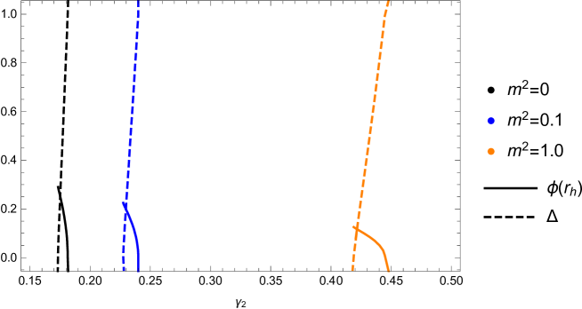
Figure 4: The value $\phi^{\prime}(r_{h})$ and the quantity $\Delta$ as function of $\gamma_{2}$ for several values of $\gamma_{1}$ for the solutions with $r_{h}=1$.

The shift to larger values of the interval of $\gamma_{2}$ while increasing $m$ can be understood by examining the field equation of the scalar field. With the assumptions made in this section (for instance : a real scalar field, a mass term only and $\gamma_{1}=0$), (2.5) reads

$$-\square\phi=2\left(\gamma_{2}\mathcal{I}(g)-m^{2}\right)\phi.$$

One can see that the mass act as a “negative shift constant” on the term $\gamma_{2}\mathcal{I}(g)$. For $m=0$ the scalarised solutions appears only when the Gauss-Bonnet term becomes sufficiently important (i.e. when $\gamma_{2}$ is large enough to ensure the term $\mathcal{I}(g)$ to trigger the scalar field). It is then intuitive to assert that, since the mass just shift down the trigger term of the scalar field, higher values of $\gamma_{2}$ are needed to allow for spontaneous scalarisation.

4 Boson stars

As we mentionned in Sect. 2, it is well known (see e.g. [16]) that regular solutions – boson stars – exist within a large subclass of the lagrangian (2.1). Let us first specify the conditions :

• The scalar field is complex, of the form (2.8) with $\omega\neq 0$. Accordingly, the Lagrangian possesses a $U(1)$-global symmetry.

• The linear coupling to the Gauss-Bonnet term will be set to zero so $\gamma_{1}=0$ in (2.3). This is because we want to limit ourselves to a polynomial lagrangian in $\phi$.

• The potential should contain at least a mass term, so $m>0$ in (2.2).

Asymptotically, the functions $N(r),\phi(r)$ behave according to

$$N(r)=1-\frac{2M}{8\pi r}+O(1/r^{2})\ \ \ ,\ \ \ \phi(r)\propto\exp(-r\sqrt{m^{2}-\omega^{2}})\ \ ,$$ (4.20)

contrasting with (3.13). The exponential decay of the scalar field demonstrates the crucial role of frequency parameter $\omega$ and of the mass $m$; in particular boson stars exist for $\omega<m$. Beside the mass $M$, the solutions are further characterized by the Noether charge associated to the U(1)-symmetry of the Lagrangian. The Noether current and the calculation of the charge $Q$ can be found in numerous papers (see e.g.[24]), for brevity we give the final form of the integral to be computed to evaluate the charge :

$$Q=8\pi\omega\int\frac{r^{2}\phi^{2}}{N\sigma}\mathrm{d}r.$$ (4.21)

This quantity is interpreted as the number of elementary bosons of mass $m$ constituting the star .

The construction of boson stars is achieved by solving the field equations of Sect. 2.2 for $r\in[0,\infty]$. The regularity at the origin, the asymptotic flatness and the localization of the scalar field imply the following set of boundary conditions :

$$N(0)=1\ \ ,\ \ \phi(0)=F_{0}\ \ ,\ \ \phi^{\prime}(0)=0\ \ ,\ \ A(r\to\infty)=1\ \ ,\ \ \phi(r\to\infty)=0\$$ (4.22)

which determine the boundary value problem. Practically, the value $F_{0}$ at the center is used as control parameter in the numerical resolution; the frequency $\omega$ has to be fine-tuned as a function of $F_{0}$ for all boundary conditions to be obeyed. The frequency $\omega$, the mass $M$ and the Noether charge $Q$ can then be evaluated as functions of $F_{0}$.

4.1 Solutions without self-interaction

Let us first discuss the solutions for a pure mass potential (i.e. for $\lambda_{4}=\lambda_{6}=0$ in (2.2)). The minimally coupled boson stars (i.e. corresponding to $\gamma_{2}=0$) exist on a finite interval of the frequency $\omega/m$, that is to say for $\omega/m\in[\omega_{\min}/m,1.0]$ with $\omega_{\min}/m\approx 0.76$. The plot of the mass $M$ versus $\omega$ presents the form of a spiral as shown by the red line on Fig. 5. From this pattern, it results that two or more solutions can exist with the same frequency on specific sub-intervals of $\omega$. The vacuum (i.e. Minkowski space-time) is approached for $F_{0}\to 0$ which coincides with the limit $\omega/m\to 1$. The phenomenon limiting the boson stars in the center of the spiral is the following : while increasing $F_{0}$ the effects of gravity get stronger at the center of the lump, in particular the value $\sigma(0)$ decreases, finally approaching zero. Correspondingly the value $R(0)$ of the Ricci scalar gets arbitrarily large and a configuration with a singularity at the center is approached.

We now discuss the influence of the non-minimal coupling (i.e. with $\gamma_{2}>0$) on this pattern. A look at Fig. 5 reveals that the $M$ versus $\omega$ curve has the tendency to unwind for $\gamma_{2}>0$ and that the boson stars exist on a larger interval of $\omega$.

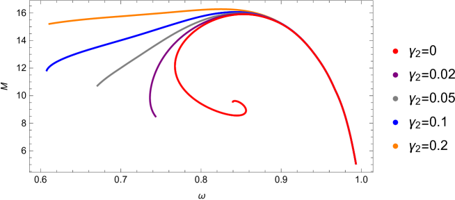
Figure 5: The mass of the boson star as a function $\omega$ for no-selfinteraction and for different values of $\gamma_{2}$.

The nature of the phenomenon limiting the curves corresponding to $\gamma_{2}>0$ on Fig. 5 is different from the case $\gamma_{2}=0$ mentionned above. Denoting $D(r)$ the denominator of the function $F_{3}$ in (2.9), it turns out that the values $\sigma(0)$, $D(0)$ both decrease when $F_{0}$ increases. However the numerical results strongly indicate that $D(0)$ tends to zero much quicker than $\sigma(0)$ once $\gamma_{2}>0$. This statement is hard to demonstrate because the numerical integration of the equations becomes particularly tricky in this limit. Within the coordinate system used both the numerator and denominator entering in $F_{3}$ become quite large in a region of the interval of integration and the accuracy of the numerical solution get lost. The situation is illustrated on Fig. 6 where the pattern of the solutions is shown in the $\omega-\sigma(0)$ plane (left-figure) and in the $\omega-\frac{D(0)}{D(\infty)}10^{9}$ plane (right-figure). In this plot, the quantity $D(r)$ has been normalized with respect to $D(\infty)$ in order to compare the curves for the different values of $\gamma_{2}$ considered. The logarithmic scale used on the vertical axis of the right plot illustrates the huge variation of $D(r)$ while approaching the critical configuration. The two plots confirm that for, $\gamma_{2}\neq 0$, the limit of existence of the boson stars is related to the behaviour of $D(0)$, rather than to $\sigma(0)$ whose values remain finite.

Note that the unwinding phenomenon of the $\omega-M$ relation seems to be closely related to the Gauss-Bonnet term. It was first observed in the construction of boson stars in Einstein-Gauss-Bonnet gravity in five dimensions [25]. In this case, the Gauss-Bonnet term is fully dynamic and does not need coupling to extra field.

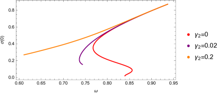
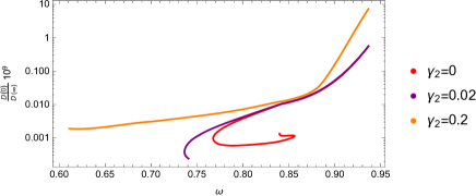
Figure 6: The value $\sigma(0)$ as function of $\omega$ for boson stars and three values of $\gamma_{2}$. Right : Idem for the discriminant of the system of equations.

4.2 Effect of a self-interacting term

Because the self-interacting potential depends on two independant parameters (namely $\lambda_{4},\lambda_{6}$), we limited the investigation to the potential of the form : $V=\phi^{2}(1-\phi^{2})^{2}$. Presenting three degenerate vacua ($\phi=0,\pm 1$), this potential offers rich possibilities for topological solitons [26]. Recently it was used in [27] for the study of kink-anti-kink collisions in 1+1 dimensions and in [28] to study boson stars in 3+1 dimensions.

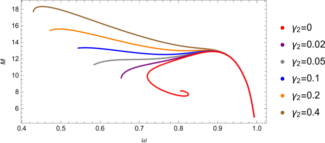
Figure 7: The mass of the boson star as a function $\omega$ for a self-interacting potential.

The general effect of the self-interacting potential on the solutions is that the interval of frequencies of the boson stars is significantly larger that for the mass potential. Especially the minimal value $\omega_{\min}$ is systematically lower (e.g. $\omega_{\min}\approx 0.72$ for $\gamma_{2}=0$). These features are illustrated by Fig. 7, to be compared with Fig. 5. The unwinding feature of the mass-frequency graphic occurring for the mass potential also takes place when the self-interaction is present. The minimal value $\omega_{\min}$ is again systematically lower although remaining strictly positive. The combination of self-interacting scalar field and non-minimal coupling to the Gauss-Bonnet term is therefore not suitable to allow for purely real soliton solutions.

One can also note that, in the presence of the self-interaction, an increase of $\gamma_{2}$ can lead to solutions with drastically higher mass compared to solutions with $\gamma_{2}=0$ (compare, for exemple, the difference between the curves corresponding to $\gamma_{2}=0$ (red) and $\gamma_{2}=0.2$ (orange) on Fig. 5 and Fig. 7).

4.3 Classical stability

We now address the stability of the boson stars by invoking a “classical argument”. With the interpretation of $Q$ as the number of bosons of mass $m$ in the lump, it is natural to compare the quantity $mQ$ to the total mass of the solution $M$. If $M<mQ$, the total mass of the boson star is lower than the sum of its components, i.e. the total energy of the system is lower than the energy corresponding to $Q$ “free” bosons. In such a case, as for the mass defect in atoms, we will say that the system is stable, in the sense that the $Q$ bosons can’t exist in a “free” form but have to be bounded within the star. Following the same lines, the case $M>mQ$ will correspond to unstable configurations (remember $m=1$ as fixing our scale, see section 2.3.4).

The quantity $M/Q$ is reported as a function of $\omega$ on Fig. 8 for several values of $\gamma_{2}$. The left part of Fig. 8 characterizes solutions with the mass term only. We see that the solutions emerging from the vacuum limit (i.e. $\omega/m=1$) are classically stable and remain so for sufficiently high values of $\omega$, say for $\omega\geq\omega_{s}$ where $\omega_{s}$ is such that $M/Q=1$. For values of $\omega$ such that several solutions coexist, the most massive is the most stable.

The most interesting result concern the influence of $\gamma_{2}$ on this pattern. As one can see on the plot, $\omega_{s}$ decreases when $\gamma_{2}$ increases while, for fixed $\omega$, $M/Q$ decreases when $\gamma_{2}$ increases. Consequently, the presence of the interaction between the scalar field and the geometry enhance the stability of the solutions.

This feature remains qualitatively the same for self-interacting solutions as illustrated on the right part of the figure. The presence of the self-interaction reinforces the effects of the curvature and the boson stars are even more stable compared to non-self-interacting ones. For sufficently high values of $\gamma_{2}$ (say for $\gamma_{2}>0.075$), the whole set of solutions is classically stable.

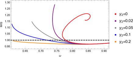
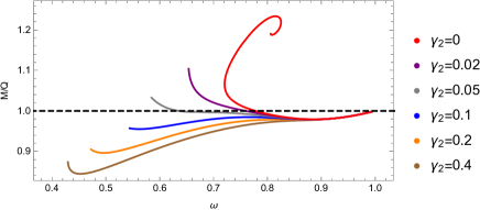
Figure 8: Left : The quantity $M/Q$ as function of $\omega$ for several values of $\gamma_{2}$ for solutions without self-interaction. Right : Idem for self-interacting solutions.

5 Conclusion

The investigation for hairy black holes in gravity extended by a Gauss-Bonnet term coupled to a scalar field was a source of huge activity over the past years. In particular the stability of such objects was examined in details in [19],[20]; the construction of such black holes in the presence of a cosmological constant was reported in [31]. The coupling function of the scalar field to the Gauss-Bonnet term is, up to now, left as an arbitrary freedom but its form lead to different patterns for the solutions and turns out to be important for the stability of the hairy black holes.

In this paper we considered as coupling a superposition of the linear and quadratic powers of the scalar field. While spontaneoulsy scalarized black holes – with purely quadratic coupling constant $\gamma_{2}$ – appear on a very limited interval of the coupling constant $\gamma_{2}$, we showed that, when adding a linear part (even with small coupling $\gamma_{1}$), two branches of hairy black holes exist. One of these branches is very close to the spontaneously scalarized black holes while the second extend backward to a solution with shift-symmetric scalar field. This feature is specific for the fundamental solutions and is not repeated for excited solution (i.e. with scalar field presenting nodes) .

Extending the scalar sector of scalar-tensor gravity to a massive, complex field, we were also able to construct boson star solutions in the full theory. The qualitative and quantitative effects of the Gauss-Bonnet term have been reported in details in Sect. 4 revealing, for instance, that the presence of the quadratic coupling constant $\gamma_{2}$ can drastically increase the maximal mass of these objects and the range of $\omega$ (the frequency of the complex scalar field) for which these solutions exist. In this context, we also show that the critical phenomenon limiting the existence of solutions is different in the minimally and non-minimally coupled case. Interestingly, our results demonstrate that the coupling to the Gauss-Bonnet invariant and/or the inclusion of a self-interacting potential of the scalar field enhances the domain of classical stability of the boson stars.

Finally, in the Appendix we studied the solutions for scalar-tensor gravity extended by the same kind of coupling of the scalar field to the Chern-Simons invariant. Here the space-time is endowed with a NUT charge. The pattern of Nutty-Hairy black holes is qualitatively similar to the Gauss-Bonnet case.

Appendix Appendix A : Coupling to the Chern-Simons invariant

In this appendix, we provide an analysis of hairy black holes in the model (2.1) where the curvature invariant is chosen as the Chern-Simons-scalar :

$${\cal I}(g)=\mathcal{L}_{CS}\equiv R\tilde{R}={\,{}^{\ast}\!}R^{a}{}_{b}{}^{cd}R^{b}{}_{acd}\ \ ,\ \ {{}^{\ast}}R^{a}{}_{b}{}^{cd}\equiv\frac{1}{2}\eta^{cdef}R^{a}{}_{bef}\,$$

where ${\,{}^{\ast}\!}R^{a}{}_{b}{}^{cd}$ is the Hodge dual of the Riemann-tensor, $\eta^{cdef}=\epsilon^{cdef}/\sqrt{-g}$ the 4-dimensional Levi-Civita tensor and $\epsilon^{cdef}$ the Levi-Civita tensor density.

The construction of classical solutions with a non-trivial Chern-Simons term can be performed by enforcing rotations in the metric or by endowing Space-Time with a NUT charge. Nutty-Hairy black holes in Einstein-Chern-Simons gravity were constructed in [29] and [21] for $\gamma_{2}=0$ and $\gamma_{1}=0$ respectively. Similar solutions within Einstein-Gauss-Bonnet (rather than Chern-Simons) gravity were obtained in [23]. The field equations are given by (2.4) and (2.5) with a different expression of $T_{\mu\nu}^{(\mathcal{I})}$ which can be found in [21] with the same notations as in Sect. 2.1.

The ansatz

To construct the solutions we use a metric of the form

$$\mathrm{d}s^{2}=-N(r)\sigma^{2}(r)(\mathrm{d}t+2n\cos\theta\mathrm{d}\varphi)^{2}+\frac{\mathrm{d}r^{2}}{N(r)}+g(r)(\mathrm{d}\theta^{2}+\sin^{2}\theta\mathrm{d}\varphi^{2})~{},$$

generalizing the Schwarzschild-NUT solution. Here $\theta$ and $\varphi$ are the standard angles on $S^{2}$ with the usual range while $r$ and $t$ are the “radial” and “time” coordinates respectivelly. The NUT parameter $n$ appears as a coefficient in the differential form $\mathrm{d}t+2n\cos\theta\mathrm{d}\varphi$ (note that $n\geqslant 0$, without any loss of generality). When evaluated with this metric, the Chern-Simons density $\mathcal{L}_{CS}$ is actually proportional to the NUT charge; so it vanishes identically for spherically symmetric solutions ($n=0$) but becomes non trivial for $n\neq 0$, ensuring a non-trivial behaviour of the scalar field via the curvature induced scalarization only for $n\neq 0$.

In the decoupling limit $\gamma_{1}=\gamma_{2}=0$ (implying $\phi=0$), the functions $N(r),\sigma(r)$ and $g(r)$ are known explicitely :

$$N(r)=1-\frac{2(Mr+n^{2})}{r^{2}+n^{2}}\ ,\qquad\sigma(r)=1\ ,\qquad g(r)=r^{2}+n^{2}\ .$$

This metric therefore possesses an horizon at

$$r_{h}=M+\sqrt{M^{2}+n^{2}}>0.$$

As in the Schwarzschild limit, $N(r_{h})=0$ is only a coordinate singularity where all curvature invariants are finite. In fact, a nonsingular extension across this null surface can be found [30]. Completing the metric (Appendix A), the ansatz for the scalar field is the same as Eq. (2.8).

Numerical results

In the same spirit as in the main part, we have constructed the black hole solutions in the Einstein-Chern-Simons (ECS) model with the mixed coupling (2.1) and using a Nutty space-time in order to make the Chern-Simons term non trivial.

For generic values of $\gamma_{1},\gamma_{2}$, no explicit solution can be found and, again, we relied on a numerical technique. For the construction, we used the gauge $\sigma(r)=1$. Then the Einstein-Chern-Simons equations can be transformed into a system of three coupled differential equations of the second order for the functions $N(r),g(r)$ and $\phi(r)$. The desired asymptotic form of the solutions require

$$N(r\to\infty)=1\ \ ,\ \ \sigma(r\to\infty)=1\ \ ,\ \ \phi(r\to\infty)=\frac{Q_{s}}{r}\$$

where $Q_{s}$ is the scalar charge. Imposing an horizon $r=r_{h}$, i.e. $N(r_{h})=0$, the conditions of regularity of the solution at the horizon can be determined on the first few coefficients of the Taylor expansion :

$$N(r)=N_{1}(r-r_{h})+O((r-r_{h})^{2})\ \ ,\ \ g(r)=g_{0}+g_{1}(r-r_{h})+O((r-r_{h})^{2})\ \ ,\ \ \phi(r_{h})=\phi_{0}+\phi_{1}(r-r_{h})+O((r-r_{h})^{2})$$

Two conditions are finally necessary :

$$g^{\prime}(r_{h})=\frac{1}{N_{1}}(2-g_{0}\phi_{0}m^{2}-2nN_{1}\phi_{1}(\gamma_{1}+2\gamma_{2}\phi_{0}))\ \ ,$$

$$24\gamma_{2}\phi_{0}^{2}\phi_{1}(N_{1})^{3}+N_{1}(2\gamma_{2}ng_{0}m^{2}\phi_{0}^{3}-12\gamma_{2}n\phi_{0}-g_{0}^{2}\phi_{1})+g_{0}^{2}\phi_{0}m^{2}=0.$$

The pattern of the solutions found for the ECS case is very similar to the case of EGB. In particular, the solutions available for non-zero values of $\gamma_{1},\gamma_{2}$ smoothly extrapolate between the limits $\gamma_{1}=0$ and $\gamma_{2}=0$ found in [21] and [29]. The results are summarized on Fig. 9 for $n=0.1$ but we have checked that they are qualitatively similar for different values of $n$.

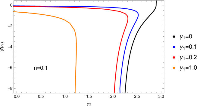
Figure 9: The value $\phi^{\prime}(r_{h})$ as function of $\gamma_{2}$ for several values of $\gamma_{1}$ for the solutions with $r_{h}=1$ and $n=0.1$.

References

- [1] G. W. Horndeski, Int. J. Theor. Phys. 10 (1974) 363.
- [2] A. Nicolis, R. Rattazzi and E. Trincherini, Phys. Rev. D 79 (2009) 064036.
- [3] C. Deffayet, X. Gao, D. A. Steer and G. Zahariade, Phys. Rev. D 84 (2011) 064039 [arXiv:1103.3260 [hep-th]].
- [4] J. D. Bekenstein, Phys. Rev. Lett. 28 (1972) 452; C. Teitelboim, Lett. Nuovo Cim. 3S2 (1972) 397.
- [5] J. D. Bekenstein, Phys. Rev. D 51 (1995) no.12, R6608.
- [6] C. A. R. Herdeiro and E. Radu, Phys. Rev. Lett. 112 (2014) 221101. [arXiv:1403.2757 [gr-qc]].
- [7] C. A. R. Herdeiro and E. Radu, Int. J. Mod. Phys. D 24 (2015) no.09, 1542014 [arXiv:1504.08209 [gr-qc]].
- [8] T. P. Sotiriou, Class. Quant. Grav. 32 (2015) no.21, 214002 [arXiv:1505.00248 [gr-qc]].
- [9] M. S. Volkov, arXiv:1601.08230 [gr-qc].
- [10] T. P. Sotiriou and S. Y. Zhou, Phys. Rev. Lett. 112 (2014) 251102 [arXiv:1312.3622 [gr-qc]].
- [11] T. P. Sotiriou and S. Y. Zhou, Phys. Rev. D 90 (2014) 124063 [arXiv:1408.1698 [gr-qc]].
- [12] D. D. Doneva and S. S. Yazadjiev, Phys. Rev. Lett. 120 (2018) no.13, 131103 [arXiv:1711.01187 [gr-qc]].
- [13] H. O. Silva, J. Sakstein, L. Gualtieri, T. P. Sotiriou and E. Berti, Phys. Rev. Lett. 120 (2018) no.13, 131104 [arXiv:1711.02080 [gr-qc]].
- [14] G. Antoniou, A. Bakopoulos and P. Kanti, Phys. Rev. Lett. 120 (2018) no.13, 131102 [arXiv:1711.03390 [hep-th]].
- [15] E. T. Newman, L.Tamburino and T. Unti, J. Math. Phys. 4 (1963) 915.
- [16] P. Jetzer, Phys. Rep. 220 (1992) 163.
- [17] F. E. Schunck and E. W. Mielke, Class. Quant. Grav. 20 (2003) R301. [arXiv:0801.0307 [astro-ph]].
- [18] G. Antoniou, A. Bakopoulos and P. Kanti, Phys. Rev. D 97 (2018) no.8, 084037. [arXiv:1711.07431 [hep-th]].
- [19] M. Minamitsuji and T. Ikeda, Phys. Rev. D 99 (2019) no.4, 044017. [arXiv:1812.03551 [gr-qc]].
- [20] H. O. Silva, C. F. B. Macedo, T. P. Sotiriou, L. Gualtieri, J. Sakstein and E. Berti, “On the stability of scalarized black hole solutions in scalar-Gauss-Bonnet gravity,” arXiv:1812.05590 [gr-qc].
- [21] Y. Brihaye, C. Herdeiro and E. Radu, Phys. Lett. B 788 (2019) 295 arXiv:1810.09560 [gr-qc].
-
[22]
U. Ascher, J. Christiansen, R. D. Russell,
Math. Comp. 33 (1979) 659;
U. Ascher, J. Christiansen, R. D. Russell, ACM Trans. 7 (1981) 209. - [23] A. Brandelet, Y. Brihaye, T. Delsate and L. Ducobu, Int. J. Mod. Phys. A 33 (2018) no.32, 1850189. [arXiv:1705.06145 [gr-qc]].
- [24] B. Kleihaus, J. Kunz and M. List, Phys. Rev. D 72 (2005) 064002. [gr-qc/0505143].
- [25] B. Hartmann, J. Riedel and R. Suciu, Phys. Lett. B 726 (2013) 906. [arXiv:1308.3391 [gr-qc]].
- [26] M. A. Lohe, Phys. Rev. D 20 (1979) 3120.
- [27] P. Dorey, K. Mersh, T. Romanczukiewicz and Y. Shnir, Phys. Rev. Lett. 107 (2011) 091602. [arXiv:1101.5951 [hep-th]].
- [28] Y. Brihaye, A. Cisterna, B. Hartmann and G. Luchini, Phys. Rev. D 92 (2015) no.12, 124061. [arXiv:1511.02757 [hep-th]].
- [29] Y. Brihaye and E. Radu, Phys. Lett. B 615 (2005) 1 [gr-qc/0502053].
- [30] S. W. Hawking and G. F. R. Ellis, “The Large Scale Structure of Space-Time,” doi:10.1017/CBO9780511524646
- [31] A. Bakopoulos, G. Antoniou and P. Kanti, “Novel Black-Hole Solutions in Einstein-Scalar-Gauss-Bonnet Theories with a Cosmological Constant,” arXiv:1812.06941 [hep-th].