Momen^et: Flavor the Moments in Learning to Classify Shapes

Abstract

A fundamental question in learning to classify 3D shapes is how to treat the data in a way that would allow us to construct efficient and accurate geometric processing and analysis procedures. Here, we restrict ourselves to networks that operate on point clouds. There were several attempts to treat point clouds as non-structured data sets by which a neural network is trained to extract discriminative properties.

The idea of using 3D coordinates as class identifiers motivated us to extend this line of thought to that of shape classification by comparing attributes that could easily account for the shape moments. Here, we propose to add polynomial functions of the coordinates allowing the network to account for higher order moments of a given shape. Experiments on two benchmarks show that the suggested network is able to provide state of the art results and at the same token learn more efficiently in terms of memory and computational complexity.

1 Introduction

In recent years the popularity and demand for 3D sensors has vastly increased. Applications using 3D sensors include robot navigation, stereo vision, and advanced driver assistance systems to name just a few. Recent studies attempt to adjust deep neural networks (DNN) to operate on 3D data representations for diverse geometric tasks. Motivated mostly by memory efficiency, our choice of 3D data representation is coordinates of point clouds. One school of thought indeed promoted feeding these geometric features as input to deep neural networks that operate on point clouds for classification of rigid objects.

From a geometry processing point of view, it is well known that moments characterize a surface and can be useful for the classification task. To highlight the importance of moments as class identifiers, we first consider the case of a continuous surface. In this case, geometric moments uniquely characterize an object. Furthermore, a finite set of moments is often sufficient as a compact signature that defines the surface [1]. This idea was classically used for estimation of surface similarity. For example, if all moments of two surfaces are the same, the surfaces are considered to be identical. Moreover, sampled surfaces, such as point clouds, can be identified by their estimated geometric moments, where it can be shown that the error introduced by the sampling is proportional to the sampling radius and uniformity.

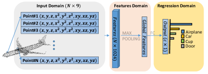
Figure 1: Illustration of the proposed object classification architecture. The input of the network includes the point cloud coordinates as well as second order polynomial functions of these coordinates. It enables the network to efficiently learn the shape moments.

Our goal is to allow a neural network to simply lock onto variations of geometric moments. One of the main challenges of this approach is that training a neural network to approximate polynomial functions requires the network depth and complexity to be logarithmically inversely proportional to the approximation error [2]. In practice, in order to approximate polynomial functions of the coordinates for the calculation of geometric moments the network requires a large number of weights and layers. Qi et al. [3] proposed a network architecture which processes point clouds for object classification. The framework they suggested includes lifting the coordinates of each point into a high dimensional learned space, while ignoring the geometric structure. An additional pre-processing transformation network was supposed to canonize a given point cloud, yet it was somewhat surprising to discover that the transformer results are not invariant to the given orientations of the point cloud. Learning to lift into polynomial spaces would have been a challenge using the architecture suggested in [3]. At the other end, networks that attempt to process other representations of low dimensional geometric structures such as meshes, voxels (volumetric grids), and multi-view projections are often less efficient when considering both computational and memory complexities.

In this paper, we propose a new network that favors geometric moments for point cloud object classification. The most prominent element of the network is supplementing the given point cloud coordinates together with polynomial functions of the coordinates, see Fig.1. This simple operation allows the network to account for higher order moments of a given shape. Thereby, the suggested network requires relatively low computational resources in terms of run-time, and memory in sense of the number of network’s parameters. Experiments on two benchmarks show that the suggested scheme is able to learn more efficiently compared to previous methods in terms of memory and actual computational complexity while providing more accurate results. Lastly, it is easy to implement the proposed concept by just calculating the polynomial functions and concatenating them as an additional vector to the current input of point cloud coordinates.

2 Related Efforts

This section reviews some early results relevant to our discussion. First, we relate to methods used for learning from processed point clouds such as voxels and trees based models. Next, we present a line of works that consume directly point clouds for object classification. The third part describes early studies of higher order networks, in which each layer applies polynomial functions to its inputs, defined by the previous layer’s output. We provide evidence that similar simple lifting ideas were applied quite successfully to geometric object recognition and classification in the late 80’s.

2.1 Learning features from processed point clouds

The most straightforward way to apply convolutional neural networks (CNNs) to 3D data is by transforming 3D models to grids of voxels, see for example [4, 5]. A grid of occupancy voxels is produced and used as input to a 3D CNN. This approach has produced successful results, but has some disadvantages such as loss of spatial resolution, and the use of excessively large memory. For some geometric tasks that require analysis of fine details, in some cases, implicit (voxel) representation would probably fail to capture fine features. Several methods replace the grid occupancy representation with radial basis functions [6], fisher vectors [7] and mean points [8] for convolving with 3D kernels. However, the 3D grid representation has an inherent drawback in terms of memory consumption.

KdNet [9] and OcNet [10] approaches exploit tree models to build a balanced and unbalanced (respectively) hierarchical structure partitions as a prepossessing stage. Nevertheless, rotation, noise or variation in number of points force rebuilding those trees from scratch.

In contrast to the methods mentioned above which encode point clouds in trees or in voxels, our method consumes the points directly.

2.2 Learning features directly from point clouds

A deep neural network applied to point clouds known as pointNet was introduced in [3]. That architecture processes the points’ coordinates for classification and segmentation. The classification architecture is based on fully connected layers and symmetry functions, like max pooling, to establish invariance to potential permutations of the points. In addition, all Multi-Layer Perceptrons (MLPs) operations are performed per point, thus, interrelations between points are accomplished only by weight sharing. Furthermore, the pointNet architecture also contains a transformer network for coping with input transformations. It is supposed to learn a set of transformations that transform the geometric input structure into some canonical configuration, however it is computationally expensive. The architecture pipeline commences with MLPs to generate a per point feature vector, then, applies max pooling to generate global features that serve as a signature of the point cloud. Finally, fully connected layers produce output scores for each class.

PointNet’s main drawback is its limited ability to capture local structures which has lead to an extensive line of work. PointNet++ [11] extracts features in local multiscale regions and aggregates local features in hierarchical manner. RSNet [12] employs recurrent neural networks (RNN) on point clouds slices for features extraction. KC-Net [13] uses point cloud local structures by kernel correlation and graph pooling. DGCNN [14] builds a k-nearest neighbor (kNN) graph in both point and feature spaces to leverage neighborhood structures. SO-Net [15] reorganizes the point cloud into a 2D map and learns node-wise features for the map. Those methods indeed capture the local structures by explicit or handcrafted methods of encoding the local information and have achieved state of the art results in 3D shape classification and segmentation tasks. However, the use of geometry context in the form of geometric moments of 3D shapes is still absent from the literature.

2.3 Learning high order features

Multi-layer perceptron (MLP) is a neural network with one or more hidden layers of perceptron units. The output $\phi$ of such a unit with an activation function $\sigma$, previous layer’s output $\eta$ and vector of learned weights $w$ is a first order perceptron, defined as $\phi=\sigma(\sum_{j}w_{j}\eta_{j})$. Where, $\sigma$ is a sigmoid function, $\sigma(a)=1/(1+e^{-a})$.

In the late 80’s, the early years of artificial intelligence, Giles et al. [16, 17] proposed extended MLP networks called higher-order neural networks. Their idea was to extend all the perceptron units in the network to include also the sum of products between elements of the previous layer’s output $\eta$. The extended perceptron unit named high-order unit is defined as

(1)

These networks included some or all of the summation terms. Theoretically, an infinite term of single high order layer can perform any computation of a first order multi-layer network [18]. Moreover, the convergence rate using a single high layer network is higher, usually by orders of magnitude, compared to the convergence rate of a multi-layer first order network [17]. Therefore, higher-order networks are considered to be powerful, yet, at the cost of high memory complexity. The number of weights grow exponentially with the number of inputs, which is a prohibitive factor in many applications.

A special case of high order networks is the square multi-layer perceptron proposed by Flake et al. [19]. They extend the perceptron unit with only the squared components of $\eta$, given by

$$\phi = \sigma\left(\sum_{i}w_{i}\eta_{i}+\sum_{j}w_{j}\eta_{j}^{2}\right).$$ (2)

The authors have shown that with a single hidden unit the network has the ability to generate localized features in addition to spanning large volumes of the input space, while avoiding large memory requirements.

3 Methods

The main contribution of this paper is leveraging the network’s ability to operate on point clouds by adding polynomial functions to their coordinates. Such a design can allow the network to account for higher order moments and therefore achieve higher classification accuracy with lower time and memory consumption. Next, we show that it is indeed essential to add polynomial functions to the input, as learning to multiply inputs items is a challenge for neural networks.

3.1 Problem definition

The goal of our network is to classify 3D objects given as point clouds embedded in $\mathbb{R}^{3}$. A given point cloud $X$ is defined as a cloud of $n$ points, where each point is described by its coordinates in $\mathbb{R}^{3}$. That is, $X=\{{\bf x}_{1},\ldots,{\bf x}_{n}\}$, where each point ${\bf x}_{j}$, is given by its coordinates $(x_{j},y_{j},z_{j})^{T}$. The output of the network, should allow us to select the class $Y\in\mathbf{L}$, where $\mathbf{L}=\{1,\ldots,L\}$ is a set of $L$ labels. For a neural network defined by the function $g:\mathbb{R}^{n\times 3}\rightarrow\mathbb{R}^{L}$, the desired output is a score vector in $\mathbb{R}^{L}$, such that $Y=\arg\max_{l\in\mathbf{L}}g(X;l)$.

3.2 Geometric Moments

The usage of invariant moments as shape descriptors is based on the theory of invariant algebra [20] which addresses mathematical objects that remain unchanged under linear transformations. Sadjadi and Hall [21], were the first to utilize moments as 3D shape descriptors. Since the 80’s, extensive research has been done exploring moments as descriptors of shapes in two and three dimensions [22, 23, 24, 25, 26, 27].

Geometric moments of increasing order represent distinct spatial characteristics of the point cloud distribution, implying a strong support for construction of global shape descriptors. By definition, first order moments represent the extrinsic centroid; second order moments measure the covariance and can also be thought of as moments of inertia. Second order moments of a set of points $X\subseteq\mathbb{R}^{3}$ can be compactly expressed in a $3\times 3$ symmetric matrix $\Sigma$, Eq. (3). where ${\bf x}_{j}\in X$ defines a point given as a vector of its coordinates ${\bf x}_{j}=(x_{j},y_{j},z_{j})^{T}$.

$$\Sigma=\sum_{j}{\bf x}_{j}{\bf x}_{j}^{T}.$$ (3)

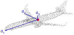
Figure 2: The first and second geometric moments displayed on a point cloud. Using the first order moments (red disc), the translation ambiguity can be removed. The principal directions $d_{1},d_{2},d_{3}$ (blue arrows) are defined by the second order geometric moments. Adding these moments to the input helps the network to resolve the rotation ambiguity.

 

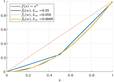
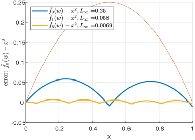
Figure 3: Approximation of the function $x^{2}$ by a fully-connected feed forward neural network $f_{n}(w)$ where $n$ denotes the number of hidden layers. Left: Approximation by different numbers of hidden layers. Right: The error of these functions.

Roughly speaking, we propose to relate between point clouds by learning to implicitly correlate their moments. Explicitly, the functions $(x^{2},y^{2},z^{2},xy,xz,yz)$ of each point are given to a neural network as input features in order to obtain better accuracy.

Geometric transformations. A desired geometric property is invariance to rigid transformations. Any rigid transformation in $\mathbb{R}^{3}$ can be decomposed into rotation and translation transformations, each defined by three parameters [1]. A rigid Euclidean transformation $T$ operating on a vector $v\in\mathbb{R}^{3}$ has the general form

$$T(v)=R\cdot v+t,$$ (4)

where $R$ is the rotation matrix and $t$ is the translation vector.

Once translation and rotation are resolved, a canonical form can be realized. The pre-processing procedure translates the origin to the center of mass given by the first order moments, and scales it into a unit sphere compensating for variations in scale. The rotation matrix, determined by three degrees of freedom, can be estimated by finding the principal directions of a given object, for example see Figure 2.

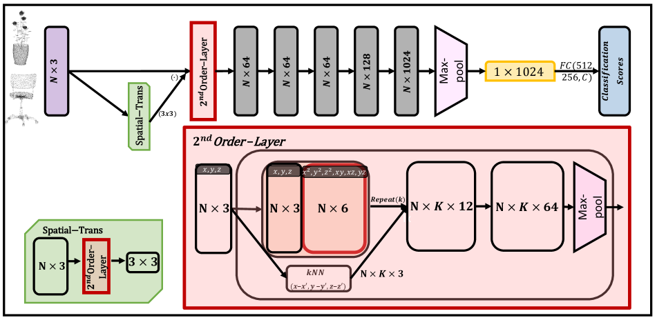
Figure 4: Momen^et Architecture. Momen^et takes as input $N$ points, applies a spatial transformation, and then aggregates the polynomial input multiplications with the k-nearest-neighbors graph as suggested in [14]. Next, point-wise MLP layers are followed by max-pooling. The output is a probability distribution over the $C$ classes. $\boldsymbol{2^{nd}}$ Order Layer aggregates each point separately with its second order polynomial expansions, then concatenates it with the point’s neighbors.

The principal directions are defined by the eigenvectors of the second order moments matrix $\Sigma$, see Eq. 3. They can be used to rotate and translate a given set of points into a canonical pose, where the axes align with directions of maximal variations of the given point cloud [28]. The first principal direction $d_{1}$, the eigenvector corresponding to the largest eigenvalue, is the axis along which the largest variance in the data is obtained. For a set of points $X\subseteq\mathbb{R}^{3}$, the $k$th direction can be found by

$$d_{k}=\operatorname*{arg\,max}_{\|d\|=1}d^{T}\left(X_{k}X_{k}^{T}\right)d,$$ (5)

where

$$X_{k}=X-\sum_{s=1}^{k-1}d_{s}d_{s}^{T}X.$$ (6)

3.3 Approximation of polynomial functions

In the suggested architecture we added low order polynomial functions as part of the input. The question arises whether a network can learn polynomial functions, obviating the need to add them manually. Here, we first provide experimental justification to the reason that one should take into account the ability of a network to learn such functions as a function of its complexity. Mathematically, we examined the ability of a network $\hat{f}(w,x)$ to approximate $f(x)$, where $w$ denotes the network parameters, such that

$$\operatorname*{arg\,min}_{\hat{f}(w,x)}\|\hat{f}(w,x)-f(x)\|_{L_{\infty}}<\epsilon,$$ (7)

for a given function $f:\mathbb{R}\rightarrow\mathbb{R}$. Theoretically, according to [29, 2], there exists a ReLU network that can approximate polynomial functions up to the above accuracy on the interval $[0,1]$, with network depth, number of weights, and computation units of $\mathcal{O}(\epsilon^{-1})$ each.

In order to verify these theoretical claims, we performed experiments to check whether a network can learn the geometric moments from the point cloud coordinates. Figure 3 shows an example for $f(x)=x^{2}$ and its approximation by a simple ReLU networks.

The pipeline can be described as follows. First we consider uniform sampling of the interval of $[0,1]$; the number of samples was chosen experimentally to be $1,000$ samples. Next, we arbitrarily chose the number of nodes in each layer to be $4$, each with ReLU activation, using fully connected layers (in contrast to the suggested network where we perform MLP separately per point). Lastly, we set the weight initialization to be taken from a normal distribution.

Ideally, networks with a larger number of layers could better approximate a given function. However, it is still a challenge to train such networks. Our experiments show that although a two layer network has achieved the theoretical bound, the network had difficulty to achieve more accurate results than $L_{\infty}=0.006$ even when we increased the number of layers above 6. Furthermore, we tried to add skip connections from the input to each node in the network; however, we did not observe a significant improvement.

Comparing two point clouds by comparing their moments is a well known method in the geometry processing literature. Yet, we have just shown that the approximation of polynomial functions is not trivial for a network. Therefore, adding polynomial functions of the coordinates as additional inputs could allow the network to learn the elements of $\Sigma$ in Eq. 3 and, assuming consistent sampling, should better capture the geometric structure of the data.

3.4 Momen^et Architecture

The network architecture is as follows (figure 4): the network takes N points as input, applies a spatial transformation resulting in a 3x3 transformation matrix. We multiply each input point with the transformation matrix to align the point cloud. Then, the transformed point cloud is fed to our second-order layer, which is a simple polynomial function of the point cloud coordinates concatenated with the point’s neighbors followed by an MLP layer. The higher order features are then processed by several point-wise MLP layers which map the points to higher dimensional space, followed by max-pooling. Finally, similarly to pointNet, we apply two fully connected layers of sizes $(512,256)$ and output a softmax over the classes.

The baseline architecture of the suggested Momen^et network is based on the pointNet architecture. Our main contribution is the addition of polynomial functions as part of the input domain. The addition of point coordinate powers to the input is a simple procedure that improves accuracy and decreases the run time during training and inference. We also calculated the k-Nearest-Neighbors (kNN) graph from the point coordinates as suggested in [14] with $k=20$. The output of the kNN block is the distance between a point to each of its $20$ neighbors, which is $(x-x^{\prime},y-y^{\prime},z-z^{\prime})$ where $(x,y,z)$ and $(x^{\prime},y^{\prime},z^{\prime})$ are the point and neighbor coordinates respectively. Then, we use a tile operation on our 2nd order polynomial expansions with the kNN output, followed by a point-wise MLP layer.

4 Experimental Analysis

4.1 Toy Problem

We first present a toy example to illustrate that extra polynomial expansions as an input can capture geometric structures well. Figure 5 (a+b) shows the data and the network predictions for $1000$ noisy 2D points, each point belongs to one of two spirals. We achieved $98\%$ success with extra polynomial multiplications, i.e $x^{2},y^{2},xy$, as input to a one layer network with only $8$ hidden ReLU nodes, contrary to the same network without the polynomial multiplications (only $53\%$ success). Figure 5(c) shows the decision boundaries that were formed from the 8 hidden nodes of network 5(b). As expected, radial boundaries can be formed from the additional polynomial extensions and are crucial to forming the entire decision surface.

(a)

(b)

(c)

Figure 5: Output response surfaces of a network comprised of 8 hidden nodes with polynomial expansions (a) and without (b). The output responses of each hidden node of (a) is presented in (c). The training set (data points) are colored in red/blue, which indicate positive/negative class respectively while orange/light blue areas are the corresponding network predictions.

4.2 Classification Performance

Dataset and data processing. Evaluation and comparison of the results to previous efforts is performed on the ModelNet40 benchmark [5]. ModelNet40 is a synthetic dataset composed of Computer-Aided Design (CAD) models, containing $12,311$ CAD models given as triangular meshes, split to $9,843$ samples for training and $2,468$ for testing. Pre-processing of each triangular mesh as proposed in [3] yields $1024$ points sampled from each triangular mesh using the farthest point sampling (FPS) algorithm. Rotation by a random angle, about the $y$ axis, and additive noise are used for data augmentation. The database contains samples of very similar categories, like the flower-pot, plant and vase, for which separation is subjective rather than objective and is a challenge even for a human observer.

Results. Table 1 shows the results of the ModelNet40 classification task for various methods that assume different representations of the data. Comparing to DGCNN, our method achieves slightly better results, doing so while using kNN only on the input points, and not on the input to all layers as in DGCNN. When DGCNN is used similarly with respect to the kNN usage, they report a significant drop in performance ($91.9\%$), this highlights the power of geometric moments as features for point clouds.

Method	Mean Class Accuracy	Overall Accuracy
PointNet [3]	86.2	89.2
Deep-Sets [30]	-	87.1
PointNet++ [11]	-	90.7
PointCNN [31]	-	91.7
ECC [32]	83.2	87.4
DGCNN [14]	90.2	92.2
Kd-Networks [9]	88.5	91.8
SO-Net [15]	87.3	90.9
KC-Net [13]	-	91.0
ShapeContexNet [33]	87.6	90.0
PCNN [6]	-	92.3
3DmFV-Net [7]	-	91.4
Momenet	90.3	92.4

Table 1: Comparison of classification accuracy (%) on ModelNet40.

4.3 Ablation Experiments

Robustness to point density and different orientations. We evaluate the robustness of our model to variations in point cloud density and to different orientations. For these tests, the model was trained in the same manner as we reported in previous sections, but was evaluated with the augmented data. Figure 6 shows results for the point density test. The model is fairly robust to sampling density variation when the ratio of dropped points is less than half.

Figure 6: Left: Point clouds with sparse to dense sampling. Right: Results of our model tested with random input dropout. The model is trained with 1024 points.

Next, we simulate different rotations of the point clouds along the y-axis. Figure 7 shows a comparison between our method and DGCNN, our model is more robust for almost all rotations when compared to DGCNN.

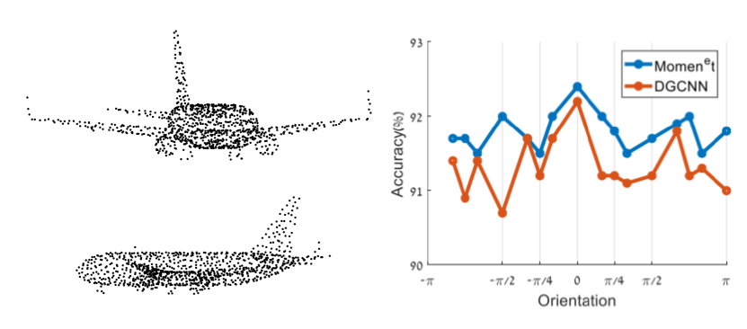
Figure 7: Left: Point clouds in different orientations. Right: Comparison of our model and DGCNN for different orientations along y-axis. The model is trained with random rotations along y-axis as DGCNN.

Variations of the Architecture. To verify the effectiveness of adding the $2^{nd}$-order layer, we test different variations in model architecture with respect to the ModelNet40 dataset. First, we examine different polynomial orders of the point cloud coordinates, see table 2. It can be seen that adding polynomial functions of order higher than $2$ does not yield improvements in performance.

Order	Overall Accuracy
$2^{nd}$	92.4
$2^{nd}+3^{rd}$	92.3
$3^{rd}$	91.9
Learnable	91.6

Table 2: Overall accuracy of modelNet40 for different order of polynomial expansions.

We also tested a variation in which the order of polynomial functions was learned by a special neural network layer defined as $exp(w\cdot log(|x|+\epsilon))$ where $w$ is the learnable kernel and $x$ is the input [34]. Second, we tested the effect of different components in our network, see table 3. Similar to our previous tests, removing the spatial transformer and reducing the number of layers in our network still achieves better accuracy than the baseline version of DGCNN ($91.2\%$).

Spatial Transformation Layers kNN Overall Accuracy ✗ [64,64,64,128,1024] ✗ 88.1 ✗ [256,1024] ✓ 91.4 ✗ [64,64,64,128,1024] ✓ 92.1 ✓ [64,64,64,128,1024] ✓ 92.4

Table 3: Variation of the network architecture. The effect of different components in our network on the accuracy with respect to ModelNet40 dataset.

   Method Memory (MB) Inference Time (msec) Acc PointNet [3] 40 5.6 89.2 PointNet++ [11] 12 10.4 90.7 DGCNN [14] 21 17.3 92.2 PCNN [6] 17 54.1 92.3 Momen^et 20 9.6 92.4

Table 4: Comparison of time and space complexity. Memory is the size of the model in mega-byte (MB) and the inference run-time was measured in milli-seconds (msec). Acc stands for the suggested network accuracy on ModelNet40.

Mean Air. Bag Cap Car Chair Ear. Guitar Knife Lamp Laptop Motor Mug Pistol Rocket Skate. Table PointNet [3] 83.7 83.4 78.7 82.5 74.9 89.6 73 91.5 85.9 80.8 95.3 65.2 93 81.2 57.9 72.8 80.6 DGCNN [14] 85.1 84.2 83.7 84.4 77.1 90.9 78.5 91.5 87.3 82.9 96.0 67.8 93.3 82.6 59.7 75.5 82.0 Kd-Net [9] 82.3 80.1 74.6 74.3 70.3 88.6 73.5 90.2 87.2 81.0 94.9 57.4 86.7 78.1 51.8 69.9 80.3 SO-Net [15] 84.9 82.8 77.8 88.0 77.3 90.6 73.5 90.7 83.9 82.8 94.8 69.1 94.2 80.9 53.1 72.9 83.0 KC-Net [13] 83.7 82.8 81.5 86.4 77.6 90.3 76.8 91.0 87.2 84.5 95.5 69.2 94.4 81.6 60.1 75.2 81.3 PCNN [6] 85.1 82.4 80.1 85.5 79.5 90.8 73.2 91.3 86.0 85.0 95.7 73.2 94.8 83.3 51.0 75.0 81.8 3DmFV-Net [7] 84.3 82.0 84.3 86.0 76.9 89.9 73.9 90.8 85.7 82.6 95.2 66.0 94.0 82.6 51.5 73.5 81.8 Momen^et 84.9 84.4 82.7 88.4 78.5 90.7 78.1 90.1 87.3 82.5 96.1 65.6 94.9 83.1 58.5 73.6 81.7

Table 5: Comparison of segmentation results on the ShapeNet database. The evaluation metric is mean Intersection over Union (IoU).

Memory and Computational Efficiency. Our network is implemented in tensorflow [35], we use ADAM optimizer [36] with initial learning rate 0.01. Table 4 presents computational requirements with respect to the number of the network’s parameters (memory) and with respect to the inference time required by the models.

The inference time is measured for one point cloud with 1024 points on nVidia Titan X GPU. In comparison with other methods, our results show that adding polynomial expansions to the input leads to better classification performance, as well as computational and memory efficiency.

4.4 Part Segmentation Performance

Dataset and data processing. Evaluation and comparison of the results to previous efforts is performed on the ShapeNet benchmark [5]. ShapeNet contains $16,881$ 3D models with $50$ annotated parts from $16$ categories. The dataset is considered challenging due to the imbalance of its labels. The aim of the part segmentation task is to predict a category label to each point in the point cloud. The splitting of the dataset to train/test and sampling of the points were done similarly to [3].

Training and test procedures. We extended our architecture to address the segmentation task, which requires local and global features. The network segmentation architecture is as follows: the network takes N points as input, applies a spatial transformation, then the transformed point cloud is fed to our second-order layer as in the classification network. The higher order point-wise features are processed by point-wise MLP layers and their outputs are concatenated to the $1024$ global features layer. Finally, we apply several point-wise MLP layers to produce a label to each point.

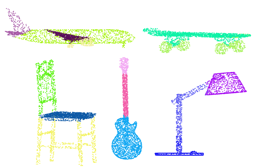
Figure 8: Qualitative results of Momen^et on the part segmentation task, performed on the ShapeNet database [5].

To reduce memory consumption, we decreased the k-nearest neighbors to only $15$, compared to $k=30$ in DGCNN. Decreasing the number of neighbors during the kNN computation also helps to substantially reduce the run-time of the network during both training and inference.

Results. The evaluation metric is mean Intersection over Union (IoU), and in order to calculate it we followed the same scheme as pointNet. We compute the IoU of each category by averaging the IoU of all the samples belonging to that category, and then average the IoU of all the categories. Lastly, we average the IoU of all the test samples to get our final performance metric. Table 5 shows detailed segmentation results on the ShapeNet dataset. Our network achieves similar results to state-of-the-art methods despite the fact that we use only $15$ neighbors, which leads to a reduction in memory consumption and run-time. Qualitative results are shown in Figure 8.

5 Conclusions

In this paper, we combined a geometric understanding about the ingredients required to construct compact shape signatures with neural networks that operate on clouds of points to leverage the network’s abilities to cope with the problem of rigid objects classification. By lifting the shape coordinates into a small dimensional, moments-friendly space, the suggested network, Momen^et, is able to learn more efficiently in terms memory and computational complexity and provide more accurate classifications compared to related methods. Experimental results on two benchmark datasets confirm the benefits of such a design. We demonstrated that lifting the input coordinates of points in $\mathbb{R}^{3}$ into $\mathbb{R}^{9}$ by simple second degree polynomial expansion, allowed the network to lock onto the required moments and classify the objects with better efficiency and accuracy compared to previous methods that operate in the same domain. We showed experimentally that it is beneficial to add these expansions for the classification and the segmentation tasks. We believe that the ideas introduced in this paper could be applied in other fields where geometry analysis is involved, and that the simple cross product of the input point with itself could improve networks abilities to efficiently and accurately handle geometric structures.

References

- [1] Alexander M Bronstein, Michael M Bronstein, and Ron Kimmel. Numerical geometry of non-rigid shapes. Springer Science & Business Media, 2008.
- [2] Dmitry Yarotsky. Error bounds for approximations with deep relu networks. Neural Networks, 94:103--114, 2017.
- [3] Charles R Qi, Hao Su, Kaichun Mo, and Leonidas J Guibas. Pointnet: Deep learning on point sets for 3d classification and segmentation. Proc. Computer Vision and Pattern Recognition (CVPR), IEEE, 1(2):4, 2017.
- [4] Daniel Maturana and Sebastian Scherer. Voxnet: A 3d convolutional neural network for real-time object recognition. In Intelligent Robots and Systems (IROS), 2015 IEEE/RSJ International Conference on, pages 922--928. IEEE, 2015.
- [5] Zhirong Wu, Shuran Song, Aditya Khosla, Fisher Yu, Linguang Zhang, Xiaoou Tang, and Jianxiong Xiao. 3d shapenets: A deep representation for volumetric shapes. In Proceedings of the IEEE conference on computer vision and pattern recognition, pages 1912--1920, 2015.
- [6] Matan Atzmon, Haggai Maron, and Yaron Lipman. Point convolutional neural networks by extension operators. ACM Trans. Graph., 37(4):71:1--71:12, July 2018.
- [7] Yizhak Ben-Shabat, Michael Lindenbaum, and Anath Fischer. 3dmfv: Three-dimensional point cloud classification in real-time using convolutional neural networks. IEEE Robotics and Automation Letters, 3(4):3145--3152, 2018.
- [8] Binh-Son Hua, Minh-Khoi Tran, and Sai-Kit Yeung. Pointwise convolutional neural networks. In Proceedings of the IEEE Conference on Computer Vision and Pattern Recognition, pages 984--993, 2018.
- [9] Roman Klokov and Victor Lempitsky. Escape from cells: Deep kd-networks for the recognition of 3d point cloud models. In Computer Vision (ICCV), 2017 IEEE International Conference on, pages 863--872. IEEE, 2017.
- [10] Gernot Riegler, Ali Osman Ulusoy, and Andreas Geiger. Octnet: Learning deep 3d representations at high resolutions. In Proceedings of the IEEE Conference on Computer Vision and Pattern Recognition, pages 3577--3586, 2017.
- [11] Charles Ruizhongtai Qi, Li Yi, Hao Su, and Leonidas J Guibas. Pointnet++: Deep hierarchical feature learning on point sets in a metric space. In Advances in Neural Information Processing Systems, pages 5105--5114, 2017.
- [12] Qiangui Huang, Weiyue Wang, and Ulrich Neumann. Recurrent slice networks for 3d segmentation of point clouds. In Proceedings of the IEEE Conference on Computer Vision and Pattern Recognition, pages 2626--2635, 2018.
- [13] Yiru Shen, Chen Feng, Yaoqing Yang, and Dong Tian. Mining point cloud local structures by kernel correlation and graph pooling. In Proceedings of the IEEE conference on computer vision and pattern recognition, pages 4548--4557, 2018.
- [14] Yue Wang, Yongbin Sun, Ziwei Liu, Sanjay E Sarma, Michael M Bronstein, and Justin M Solomon. Dynamic graph cnn for learning on point clouds. arXiv preprint arXiv:1801.07829, 2018.
- [15] Jiaxin Li, Ben M Chen, and Gim Hee Lee. So-net: Self-organizing network for point cloud analysis. In Proceedings of the IEEE conference on computer vision and pattern recognition, pages 9397--9406, 2018.
- [16] C Lee Giles and Tom Maxwell. Learning, invariance, and generalization in high-order neural networks. Applied optics, 26(23):4972--4978, 1987.
- [17] C Lee Giles, RD Griffin, and T Maxwell. Encoding geometric invariances in higher-order neural networks. In Neural information processing systems, pages 301--309, 1988.
- [18] YC Lee, Gary Doolen, HH Chen, GZ Sun, Tom Maxwell, and HY Lee. Machine learning using a higher order correlation network. Technical report, Los Alamos National Lab., NM (USA); Maryland Univ., College Park (USA), 1986.
- [19] Gary William Flake. Square unit augmented radially extended multilayer perceptrons. In Neural Networks: Tricks of the Trade, pages 145--163. Springer, 1998.
- [20] John Hilton Grace and Alfred Young. The algebra of invariants. Chelsea Pub. Co., 1903.
- [21] Firooz A Sadjadi and Ernest L Hall. Three-dimensional moment invariants. IEEE Transactions on Pattern Analysis and Machine Intelligence, (2):127--136, 1980.
- [22] Ming-Kuei Hu. Visual pattern recognition by moment invariants. IRE transactions on information theory, 8(2):179--187, 1962.
- [23] Yaser S Abu-Mostafa and Demetri Psaltis. Recognitive aspects of moment invariants. IEEE Transactions on Pattern Analysis & Machine Intelligence, (6):698--706, 1984.
- [24] Firooz A Sadjadi and Ernest L Hall. Numerical computations of moment invariants for scene analysis. In Proceedings of the IEEE Conference on Pattern Recognition and Image Processing, pages 127--136, 1978.
- [25] C-H Teh and Roland T Chin. On image analysis by the methods of moments. In Proceedings CVPR’88: The Computer Society Conference on Computer Vision and Pattern Recognition, pages 556--561. IEEE, 1988.
- [26] Alireza Khotanzad and Yaw Hua Hong. Invariant image recognition by zernike moments. IEEE Transactions on pattern analysis and machine intelligence, 12(5):489--497, 1990.
- [27] Anthony P. Reeves, Richard J Prokop, Susan E. Andrews, and Frank P. Kuhl. Three-dimensional shape analysis using moments and fourier descriptors. IEEE Transactions on Pattern Analysis and Machine Intelligence, 10(6):937--943, 1988.
- [28] NA Campbell and William R Atchley. The geometry of canonical variate analysis. Systematic Biology, 30(3):268--280, 1981.
- [29] Shiyu Liang and R Srikant. Why deep neural networks for function approximation? Proceedings of the International Conference on Learning Representations (ICLR), 2017.
- [30] Manzil Zaheer, Satwik Kottur, Siamak Ravanbakhsh, Barnabas Poczos, Ruslan R Salakhutdinov, and Alexander J Smola. Deep sets. In Advances in neural information processing systems, pages 3391--3401, 2017.
- [31] Yangyan Li, Rui Bu, Mingchao Sun, and Baoquan Chen. Pointcnn. arXiv preprint arXiv:1801.07791, 2018.
- [32] Martin Simonovsky and Nikos Komodakis. Dynamic edgeconditioned filters in convolutional neural networks on graphs. In Proc. CVPR, 2017.
- [33] Saining Xie, Sainan Liu, Zeyu Chen, and Zhuowen Tu. Attentional shapecontextnet for point cloud recognition. In Proceedings of the IEEE Conference on Computer Vision and Pattern Recognition, pages 4606--4615, 2018.
- [34] Andrew Trask, Felix Hill, Scott E Reed, Jack Rae, Chris Dyer, and Phil Blunsom. Neural arithmetic logic units. In Advances in Neural Information Processing Systems, pages 8046--8055, 2018.
- [35] Martín Abadi, Paul Barham, Jianmin Chen, Zhifeng Chen, Andy Davis, Jeffrey Dean, Matthieu Devin, Sanjay Ghemawat, Geoffrey Irving, Michael Isard, et al. Tensorflow: A system for large-scale machine learning. In 12th USENIX Symposium on Operating Systems Design and Implementation (OSDI 16), pages 265--283, 2016.
- [36] Diederik P Kingma and Jimmy Ba. Adam: A method for stochastic optimization. arXiv preprint arXiv:1412.6980, 2014.