Estimating QCD uncertainties in Monte Carlo event generators for gamma-ray dark matter searches

Abstract

Motivated by the recent galactic center gamma-ray excess identified in the Fermi-LAT data, we perform a detailed study of QCD fragmentation uncertainties in the modeling of the energy spectra of gamma-rays from Dark-Matter (DM) annihilation. When Dark-Matter particles annihilate to coloured final states, either directly or via decays such as $W^{(*)}\to q\bar{q}^{\prime}$, photons are produced from a complex sequence of shower, hadronisation and hadron decays. In phenomenological studies their energy spectra are typically computed using Monte Carlo event generators. These results have however intrinsic uncertainties due to the specific model used and the choice of model parameters, which are difficult to asses and which are typically neglected. We derive a new set of hadronisation parameters (tunes) for the Pythia 8.2 Monte Carlo generator from a fit to LEP and SLD data at the $Z$ peak. For the first time we also derive a conservative set of uncertainties on the shower and hadronisation model parameters. Their impact on the gamma-ray energy spectra is evaluated and discussed for a range of DM masses and annihilation channels. The spectra and their uncertainties are also provided in tabulated form for future use. The fragmentation-parameter uncertainties may be useful for collider studies as well.

1 Introduction

The existence of Dark Matter (DM), making up $\sim 85\%$ of the matter of the universe, is today an accepted part of the Standard Cosmological Model. Observations of cosmological large scale structure moreover favour that the DM was not relativistic when galaxies formed, the so called cold DM (CDM) scenario.

In particle physics, the CDM scenario is most straightforwardly realised by extending the Standard Model (SM) with weakly interacting massive particles (WIMPs). Unlike neutrinos, WIMPs can be non-relativistic and hence compatible with the CDM scenario. They can also provide a simple and compelling explanation of the density of DM we observe today in the Universe through a thermal mechanism Bertone:2004pz . Namely, WIMPs were in thermal equilibrium with the thermal bath when the temperature of the plasma was larger than their mass. As long the temperature was dropping their number density was decreasing due to the cooling of the Universe. Eventually they froze out due to the expansion of the Universe and the comoving number density was fixed. What is interesting is that weak interactions and WIMP masses $\sim 100$ GeV give rise to the relic abundance of DM observed by the Planck satellite ($\Omega_{DM}h^{2}=0.1188\pm 0.0010$) Ade:2015xua . This is the so-called WIMP miracle.

WIMPs could be detected indirectly through annihilation to gamma-rays, positrons, antiprotons, neutrinos and other particles that can be observed in experiments such as the Fermi Large Area Telescope (LAT), AMS-02 or IceCube. Those annihilation products might leave footprints in the fluxes of cosmic rays and any excess could be interpreted as a WIMP signature. This is the case of the excess detected in the gamma-ray data collected by the Fermi-LAT from the inner Galaxy TheFermi-LAT:2015kwa , the so-called Galactic Center Excess (GCE). Its spectral energy distribution and morphology are consistent with predictions from DM annihilation Goodenough:2009gk ; Vitale:2009hr ; Hooper:2010mq ; Gordon:2013vta ; Hooper:2011ti ; Daylan:2014rsa ; Calore:2014xka ; Abazajian:2014fta ; Zhou:2014lva .

There have been many attempts to explain the GCE in the particle physics framework, particularly in the supersymmetry context Caron:2015wda ; 2015arXiv150707008B ; Butter:2016tjc ; Achterberg:2017emt . In its minimal phenomenological realization, called the Minimal Supersymmetric Standard Model, it has been shown that the precision in the determination of the gamma-ray spectrum from DM annihilation plays a fundamental role in the quality of fitting the model to the data Caron:2015wda .

For dark-matter annihilation processes that produce hadronic final states — either directly or via the hadronic decays of intermediate resonances like $W$, $Z$, or $H$ bosons — the dominant source of particle production is QCD jet fragmentation (for dark-matter masses above a few GeV). Long-lived particles such as photons are then produced as the final result of a complex sequence of physical processes which include bremsstrahlung, hadronisation, and hadron decays. There is no first-principles solution to the problem of hadronisation. However, by exploiting that it is a long-distance effect, as compared to the scales involved in typical high-energy (sub-femtometre) production processes, it can be formally factorised off in a universal (process-independent) way and represented either by parametric fits (called Fragmentation Functions, or FFs for short; see Metz:2016swz ) or by explicit dynamical models, such as the string Artru:1974hr ; Andersson:1983ia or cluster Webber:1983if ; Winter:2003tt models which are embedded in Monte Carlo (MC) event generators Buckley:2011ms . Note that the former (FFs) typically only parametrise the spectra of one specific type of particle at a time, with all other degrees of freedom inclusively summed over. This allows to reach a higher formal accuracy, albeit typically only over a limited range in the energy fraction of the produced hadrons. In contrast, the MC models provide fully exclusive simulated “events” from which in principle any desired observable can be constructed, with formally less accuracy but typically a broader range of applicability. In both formalisms, the essential point is that the parameters governing the long-distance physics are to a good approximation independent of the detailed nature of the short-distance process; they can therefore be constrained by fits to data (such as $e^{+}e^{-}\to\mbox{hadrons}$) and applied universally to make predictions for other processes (such as dark-matter annihilation).

In the context of such predictions, a crucial question is what is the uncertainty on the predicted spectra? A recent comprehensive study Cembranos:2013cfa highlighted that different MC models make different default assumptions for which physics effects to include and over which dynamical ranges; this can result in large differences in particular in the tails of distributions, e.g. for very low photon energies (for which it becomes important whether and how photon radiation off hadrons is treated, and/or how soft radiation off leptons is regulated) or for very high photon energies (for which prompt QED bremsstrahlung, $q\to q\gamma$, dominates). However the study also showed that in the bulk of the distributions, well inside these limits, there was a high level of agreement between the codes. This agrees with what one would expect from the default parameter sets for the MC models being chosen to essentially provide “central” fits to roughly the same set of constraining data, comprised mostly of LEP measurements; see Buckley:2009bj ; Buckley:2010ar ; Skands:2010ak ; Platzer:2011bc ; Karneyeu:2013aha ; Skands:2014pea ; Fischer:2014bja ; Fischer:2016vfv ; Reichelt:2017hts ; Kile:2017ryy . This degeneracy of fitting different models to the same data, however, also implies that the envelope spanned by them is not a particularly systematic or exhaustive way of exploring the true region of allowed uncertainty. Thus, while there can be huge differences in the tails caused by intrinsically different modeling assumptions, we believe that the uncertainty in the bulk of the distributions is not well represented by the envelope of different MC models, or is at least not guaranteed to be well represented by it.

The question we wish to address in this paper is therefore: can we provide meaningful and exhaustive sets of alternative model parameters that are able to faithfully represent the uncertainty with respect to a given set of constraining measurement data, within a given modeling paradigm? To answer this question, we take the default Monash 2013 tune Skands:2014pea of the Pythia 8 event generator Sjostrand:2014zea as our baseline and — using a selection of fragmentation constraints from $e^{+}e^{-}$ colliders encoded in the Rivet Buckley:2010ar analysis preservation package combined with the Professor Buckley:2009bj parameter optimisation tool — define a small set of systematic parameter variations which we argue explores the uncertainty envelopes relevant for estimating QCD fragmentation uncertainties on dark-matter annihilation processes in a meaningful way, and could be useful for estimating at least the flavour-insensitive component of fragmentation uncertainties on collider observables as well. As will be discussed in the main part of the paper, a straightforward $\chi^{2}$ minimisation with uncertainty envelopes defined by parameter variations along the eigenvectors corresponding to $\Delta\chi^{2}=1$ variations (called “eigentunes” Buckley:2009bj ) does not immediately result in what we could call a faithful representation of the true uncertainty envelope, but with minor and well-motivated modifications can be adapted to produce such representations.

The paper is organized as follows. In Sec. 2 we describe how the photon spectra from DM annihilation is modeled in MC event generators. In Sec. 3 a detailed study of the origin of the gamma spectrum is presented while in Sec. 4 the tunning of the MC to data is performed and in Sec. 5 we present the results of the tuning and the QCD uncertainties with emphasis on the impact of those uncertainties on two benchmark points of the MSSM. We conclude in Sec. 6.

2 Physics Modeling

Consider a generic dark-matter annihilation process, $\chi\chi\to X$. Typically, we have a lowest-order picture in mind for what $X$ can be, in which additional physics (like sequential resonance decays, or fragmentation of coloured particles) are implicitly summed over. These aspects must be dealt with explicitly before final-state observables like photon spectra can be estimated.

If $X$ includes short-lived resonances such as $Z/W$ or $H$ bosons, then the narrow-width approximation allows us to factorise the complete physics process into a production part, $\chi\chi\to X_{1}\ldots X_{n}$, and a decay part, $X_{i}\to Y_{i1}\ldots Y_{in}$. This factorisation is reliable up to corrections of order $\Gamma_{i}/M_{i}$, and is hence a good approximation for states with $\Gamma\ll M$ such as the SM gauge and Higgs bosons. Note that at wavelengths above $(\hbar c)/\Gamma_{i}$, we would still expect interference effects between the decay products of different resonances, suppressed by boost effects if the resonances have non-zero relative velocities.

If $X$ (or decay products $Y$) includes photons or electrically charged particles, then those will undergo QED bremsstrahlung showers. Additional photons are produced via $X_{i}^{\pm}\to X_{i}^{\pm}\gamma$ branchings, which are enhanced for both soft (low $x_{\gamma}=E_{\gamma}/m_{\chi}$) and (quasi)collinear photons. Note that the latter type of photons can have high energies (the only requirement for the enhancement being a small angle between the photon and its parent particle) and tend to dominate the ultra-hard tail of the final-state photon spectra towards $x_{\gamma}\to 1$. Charged fermion-antifermion pairs can also be produced, at a subleading level, via $\gamma\to f\bar{f}$ branchings, which are enhanced at very low values of $Q^{2}/m_{\chi}^{2}=(p_{f}+p_{\bar{f}})^{2}/m_{\chi}^{2}$. The main modeling parameter that governs the rate of both types of QED processes is the effective value assumed for the QED fine-structure constant, $\alpha_{\mathrm{EM}}$, illustrated by fig. 1a. Nominally, this parameter is of course extremely well constrained by measurements, but it may still be useful to subject its effective value to variations, as a poor man’s way to estimate the possible effects of missing higher-order or non-universal (process-dependent) contributions to the spectra. Since this work focuses on DM annihilation to coloured particles, however, variations of $\alpha_{\mathrm{EM}}$ are quite subleading with respect to the larger variations in the QCD sector we shall discuss below, and are not considered further.

QED bremsstrahlung	QCD fragmentation and hadron decays
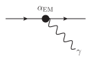
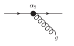
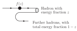
Dominates at high $x_{\gamma}$	Photons from $\pi^{0}\to\gamma\gamma$ dominate bulk (and peak) of spectra

Figure 1: Illustration of the main parameters that affect the $x_{\gamma}$ distributions in jets. From left to right: the electromagnetic coupling $\alpha_{\mathrm{EM}}$, the strong coupling $\alpha_{S}$, and the nonperturbative fragmentation function $f(z)$. For coloured final states, all three processes are active. QED bremsstrahlung is then only dominant at very high $x_{\gamma}$ where the total rate is low, while the QCD fragmentation parameters govern the bulk of the photon spectrum, via $\pi^{0}\to\gamma\gamma$ decays. (We note that $\tau\tau$ final states will also have some contributions from $\pi^{0}\to\gamma\gamma$ decays but these are controlled by the $\tau$ decay branching fractions and phase-space distributions and are independent of the $\alpha_{S}$ and $f(z)$ parameters.)

Obviously, there are also cases in which resonance decays and QED showers occur together, such as in $\chi\chi\to W^{+}W^{-}$; in an MC model like Pythia, this will be treated by first allowing the $W$ bosons to undergo QED showers, i.e. allowing for $W\to W\gamma$ branchings, with a phase space that is vanishing at the $WW$ threshold and proportional to $\Delta m_{\chi_{W}}=m_{\chi}-m_{W}$ above it. The $W$ bosons are then decayed, and their decay products undergo further showering (and hadronisation). Note that, as $m_{\chi}$ is increased, the QED shower off the $WW$ system is the only component that will become more active, due to the increasing phase space. The decays of each of the $W$ systems themselves are only affected by an overall boost (in the narrow-width limit). By Lorentz invariance, they therefore remain well constrained by measurements of decays of $W$ (or $Z$) bosons at rest as long as the range of well-measured rest-frame final-state energies still covers the region of interest in the boosted ($\chi\chi$ annihilation) frame.

If $X$ (or decay products $Y$) includes coloured particles, then those will undergo QCD showers + hadronisation. The QCD shower stage is modeled similarly to the QED one, reflecting the enhancement of soft and collinear emissions and of $g\to q\bar{q}$ splittings at low virtualities. The default treatment in Pythia is based on a combination of DGLAP splitting kernels for QED+QCD radiation with dipole ($2\to 3$) kinematics Sjostrand:2004ef . The main parameter governing the rate of QCD shower branchings is the effective value assumed for the strong coupling constant, $\alpha_{S}$, at each branching vertex, cf. fig. 1b. There are strong arguments in the literature that the renormalised coupling for shower branching processes should be evaluated at a scale proportional to the $p_{\perp}$ of each branching, and that a further set of universal corrections in the soft limit can be absorbed by using the so-called Monte Carlo, or CMW Catani:1990rr , scheme to define the running coupling, rather than the conventional $\overline{\mathrm{MS}}$ scheme. This has the net effect of increasing the effective value of $\alpha_{s}(M_{Z})$ by about 10%. In Pythia tunes, the effective value of the strong coupling is typically further increased by about 10%, to reach agreement with measured rates for $e^{+}e^{-}\to 3~{}\mathrm{jets}$; see e.g. Skands:2010ak ; Skands:2014pea . The standard recommendation for perturbative uncertainty estimates is to perform a variation of the renormalisation scale by a factor of 2 in each direction, but since this would actually destroy some of the universal corrections obtained from the CMW scheme, the framework for automated scale variations that was recently implemented in Pythia Mrenna:2016sih allows for a second-order compensation term to be imposed, which reduces the effect of the variations somewhat and reestablishes agreement with the CMW scheme at second order. This is the prescription we advocate for a realistic and still reasonably conservative uncertainty estimate on the perturbative part of the QCD fragmentation process. If desired, variations of the splitting functions by non-enhanced terms can also be included, as described in Mrenna:2016sih .

An example of a physical process that combines all of the elements of sequential resonance decays, QED showers, and QCD showers, is $\chi\chi\to t\bar{t}$. Here, the $t\bar{t}$ system will first undergo a QCD+QED shower, with a phase space proportional to how far above $t\bar{t}$ threshold the $\chi\chi$ annihilation process is. The top quarks will then decay, and the resulting $bW$ systems showered, upon which the $W$ bosons will decay, etc.

Finally, any produced coloured particles must be confined inside colourless hadrons. This process — hadronisation — takes place at a distance scale of order the proton size $\sim 10^{-15}$m and in Pythia is modelled by the Lund string model; see Andersson:1983ia for details. Since pions are the most copiously produced particles in jets and the branching fraction for $\pi^{0}\to\gamma\gamma$ is $\sim 99\%$ Patrignani:2016xqp , the vast majority of photons in jets are produced from decays of neutral pions, illustrated in fig. 2.

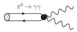
Figure 2: In hadronic jets, $\pi^{0}$ decays are the main source of photons.

The number and hardness of produced photons therefore correlates very strongly with the predicted pion spectra, and the uncertainties in turn are dominated by the quality of the available constraints on pion spectra, as well as the model’s ability to reproduce them. A crucial component of this description is the fragmentation function, $f(z)$, which parametrises the probability for a hadron to take a fraction $z\in[0,1]$ of the remaining energy at each step of the (iterative) string fragmentation process, cf. fig. 1c. While $f(z)$ cannot be calculated from first principles by current methods, its functional form is strongly constrained by self-consistency requirements (essentially, causality) within the string-fragmentation framework, so that its general form can be cast in terms of just two effective parameters, called $a$ and $b$:

$$f(z,m_{\perp h})=N\frac{(1-z)^{a}}{z}\exp\left(\frac{-bm_{\perp h}^{2}}{z}\right)~{},$$ (1)

where $N$ is a normalisation constant that ensures the distribution is normalised to unit integral, and $m_{\perp h}=\sqrt{m_{h}^{2}+p_{\perp h}^{2}}$ is called the “transverse mass”, with $m_{h}$ the mass of the produced hadron and $p_{\perp h}$ its momentum transverse to the string direction. For non-experts: if $f(z)$ is peaked near 1 (low $a$ and/or high $b$), then QCD jets will tend to consist of only a few hadrons, each taking a rather large fraction of the energy of the jet. Conversely, if $f(z)$ is peaked near zero (low $b$ and/or high $a$), then the prediction is for jets which consist of very many hadrons, each taking only a small fraction of the total available energy. An illustration of this is given in the left-hand pane of fig. 3, which shows the average number of charged particles produced in $Z\to d\bar{d}$ decays, after hadronisation, as a function of the $a$ and $b$ parameters, with all other parameters fixed to their Monash 2013 tune values Skands:2014pea . (The Monash values StringZ:aLund = 0.68 and StringZ:bLund = 0.98 are indicated by the white cross hair in the centre of the plot.)

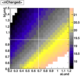
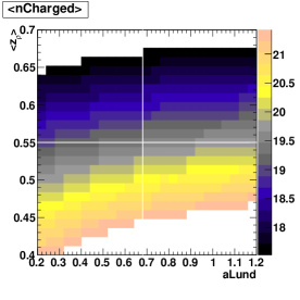
Figure 3: The average number of charged particles produced in $Z\to d\bar{d}$ decays at $E_{\mathrm{cm}}=M_{Z}=91.2$ GeV. Left: as a function of $a$ and $b$. Right: as a function of $a$ and $\left<z_{\rho}\right>$.

Since the average number of charged particles in jets is one of the most salient constraining observables, this plot also illustrates an oft-encountered problem; in tuning contexts, the $a$ and $b$ parameters are extremely highly correlated. This makes it meaningless to assign independent $\pm$ uncertainties on them; likewise sensitivity estimates and the like cannot be interpreted without taking the correlation into account carefully. Therefore, in the context of the current work, we have implemented an alternative parametrization of $f(z)$, with $b$ replaced by a parameter representing the average $z$ fraction taken by a typical hadron (specifically, primary $\rho$ mesons),

$$\left<z_{\rho}\right>=\int_{0}^{1}\mathrm{d}z\ zf(z,\left<m_{\perp\rho}\right>)~{},$$ (2)

which we solve (numerically) for $b$ at initialisation when the option StringZ:deriveBLund = on is selected in Pythia 8.235, using the following parameters:

$$\left<m_{\perp\rho}\right>^{2} = m^{2}_{\rho}+2(\mbox{{StringPT:sigma}})^{2}~{},$$ (3)

$$\left<z_{\rho}\right> = \mbox{{StringZ:avgZLund}}~{}.$$ (4)

As illustrated by the right-hand pane in fig. 3, a measurement of the mean charged multiplicity puts a rather tight bound on the value of $\left<z_{\rho}\right>$, and there is a much smaller degree of correlation with the $a$ parameter, the latter of which is essentially unconstrained by this observable. Below, this observation of reduced correlations and hence more meaningful independent $\pm$ uncertainty ranges for the new parameter set will be explored further and quantified in the context of full-fledged parameter optimisations (’tunes’).

3 Photon Origins and Measurements

3.1 Photon Origins

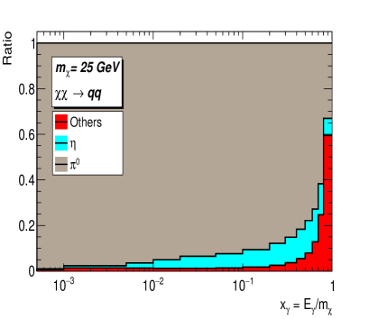
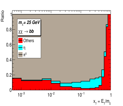
Figure 4: Ratio plots for photon origins in $\chi\chi$ annihilation into $q\bar{q},q=u,d,s$ (left panel) and $b\bar{b}$ (right panel) for $m_{\chi}=25$ GeV.

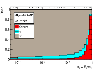
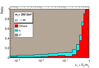
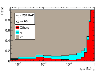
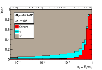
Figure 20: Contribution to $\gamma$-spectrum for dark matter annihilation into $q\bar{q}$ (top left), $c\bar{c}$ (top right), $b\bar{b}$ (bottom left) and $gg$ (bottom right) with $m_{\chi}=250$ GeV. The distribution is normalized to the total number of photons.

In the previous section, it was highlighted that the spectra of photons in QCD jets is dominated by $\pi^{0}\to\gamma\gamma$ decays. This will be studied in more details in this section. To do so, we identify the origin of photons in generic dark-matter annihilation processes with $m_{\chi}=25$ GeV and $m_{\chi}=250$ GeV. This allows the dark-matter candidate to be annihilated into quarks and gluons only for the former case and into all the SM particles in the latter case. Given that we are interested specifically in the modeling of QCD uncertainties here, final states such as $\ell^{+}\ell^{-}$ and $\gamma\gamma$ are not considered. We show in Fig. 4, the relative composition of the photon spectrum in terms of photons coming from $\pi^{0}$ decays, photons coming from $\eta^{0}$ decays, and “others” (for all other photon sources), resulting from a generic dark matter annihilation into $q\bar{q}$ and $b\bar{b}$ for $m_{\chi}=25~{}\mathrm{GeV}$. We see that the vast majority of photons indeed come from pion decays, about $95\%$ in the $q\bar{q}$ final state and $88\%$ in the $b\bar{b}$ one. The fraction is somewhat lower in the $b\bar{b}$ final state since most of these events will have one or two photons that come from $B^{*}$ decays (which are here lumped into the “others” category). However, as one goes to higher DM masses, far above the $b\bar{b}$ threshold – see Fig. 20 – the contribution from neutral pions eventually dominates again and one approaches the same distribution as in the $q\bar{q}$ case. Very subleading contributions come from photon bremsstrahlung off charged quarks; these typically dominate in the high $x_{\gamma}$ region but the total integrated rate is small. (We note however that the rate of these photons is proportional to the charge squared of the emitting particle, so there will be more such photons in $c\bar{c}$ final states, for example, than in $b\bar{b}$ ones.) On the other hand, the contribution from decays of $\eta$ mesons is about $4\%$ ($3\%$ in our $b\bar{b}$ final state example).

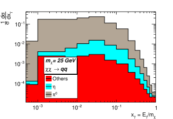
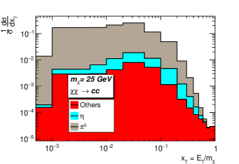
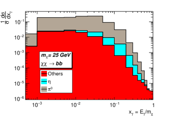
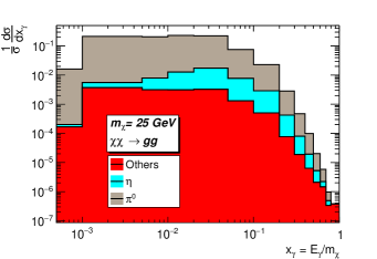
Figure 16: $\gamma$ momentum for DM annihilation into $q\bar{q}$, $c\bar{c}$, $b\bar{b}$ and $gg$ for $m_{\chi}=25$ GeV.

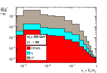
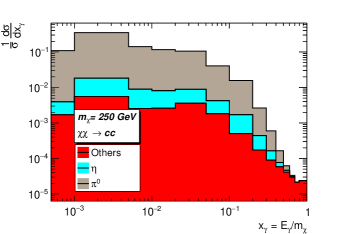
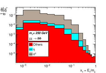
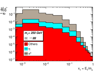
Figure 21: Same as Fig. 20 but with the differential distribution is shown.

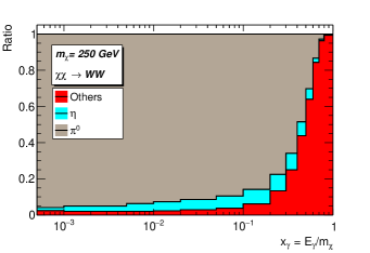
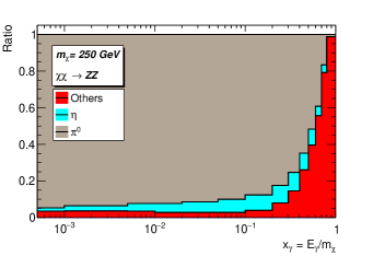
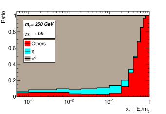
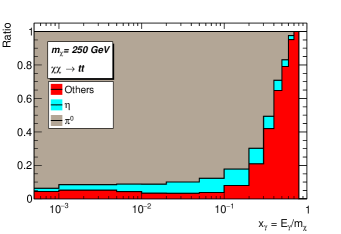
Figure 22: Same as Fig. 20 but for $WW$ (top left), $ZZ$ (top right), $hh$ (bottom left) and $t\bar{t}$ (bottom right) final states.

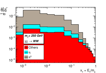
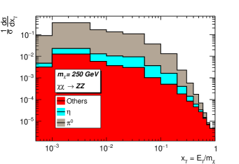
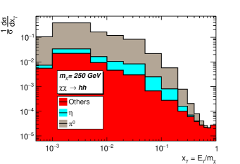
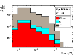
Figure 23: Same as Fig. 21 but for $WW$ (top left), $ZZ$ (top right), $hh$ (bottom left) and $t\bar{t}$ (bottom right) final states.

Photon origins in other final states and for the case of $m_{\chi}=250$ GeV are shown in the appendix specifically in Figs. 16, 20-23. For higher dark matter masses, the relative contribution of pions to the photon spectrum becomes similar in almost all final states. For other final states such as the di-Higgs, the “others” contributions occur from many sources since the full set of Higgs decay channels include not only $b\bar{b}$ but also $\tau\tau$, $c\bar{c}$, and $gg$ final states, the former three of which radiate photons before they hadronize or decay (for the case of $\tau$-leptons). Nevertheless, since this contribution is important in regions with low number of photons (see e.g Fig. 23) and, furthermore, is of QED nature, it will not affect QCD uncertainties that we estimate in what follows.

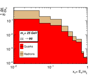
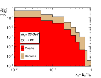
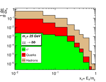
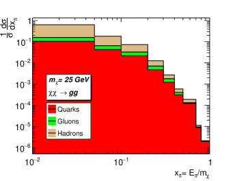
Figure 17: $\pi^{0}$ momentum for DM annihilation into $q\bar{q}$, $c\bar{c}$, $b\bar{b}$ and $gg$ for $m_{\chi}=25$ GeV.

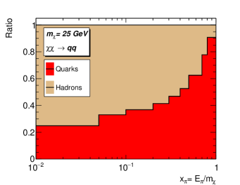
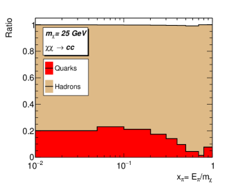
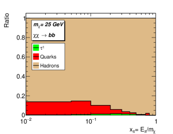
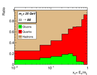
Figure 18: Different contributions to the $\pi^{0}$ scaled momentum for dark matter annihilation into $q\bar{q}$ (top left), $c\bar{c}$ (top right), $b\bar{b}$ (bottom left) and $gg$ (bottom right) for $m_{\chi}=25$ GeV.

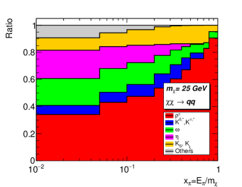
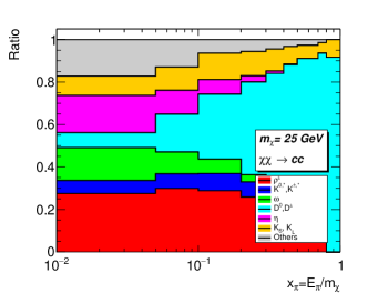
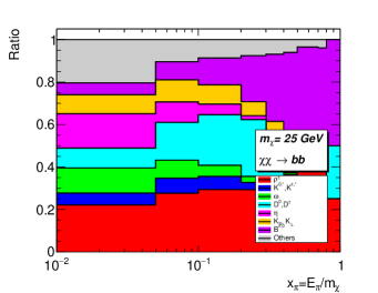
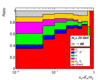
Figure 19: Same as Fig. 18 but for pions coming from hadrons

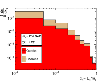
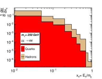
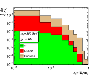
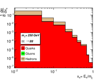
Figure 24: Same as Fig. 17 but for $m_{\chi}=250$ GeV.

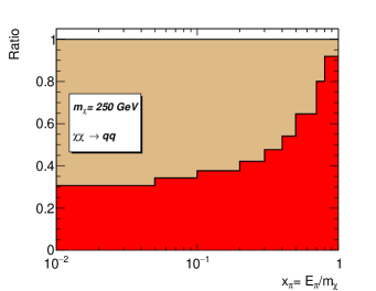
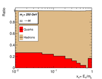
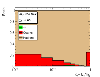
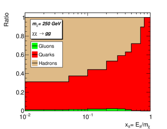
Figure 25: Same as Fig. 18 but for $m_{\chi}=250$ GeV.

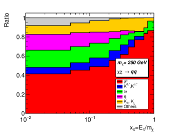
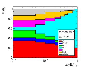
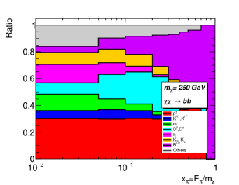
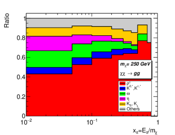
Figure 26: Same as Fig. 19 but for $m_{\chi}=250$ GeV.

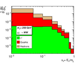
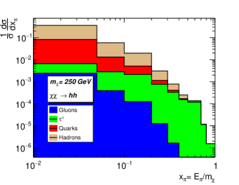
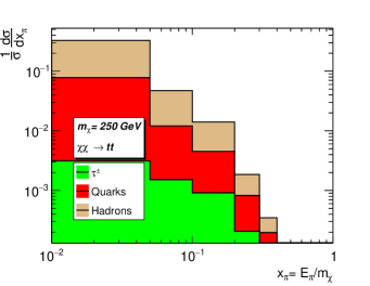
Figure 27: Same as Fig. 24 but for $WW$ (top left), $ZZ$ (top right), $hh$ (bottom left) and $t\bar{t}$ (bottom right) final states.

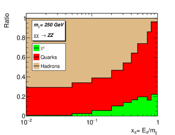
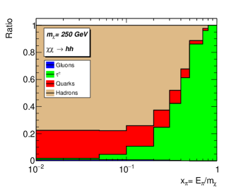
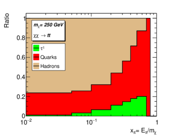
Figure 28: Same as Fig. 25 but for $WW$ (top left), $ZZ$ (top right), $hh$ (bottom left) and $t\bar{t}$ (bottom right) final states.

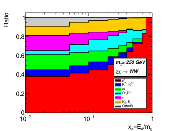
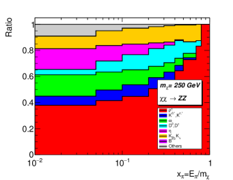
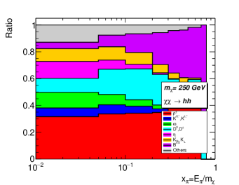
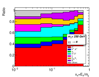
Figure 29: Same as Fig. 26 but for $WW$ (top left), $ZZ$ (top right), $hh$ (bottom left) and $t\bar{t}$ (bottom right) final states.

Given that most of the photons produced in jets come from pion decays, a study of QCD uncertainties on photon spectra ultimately boils down to a study of uncertainties on pion spectra, with a very small additional component coming from $\eta^{0}$ decays. The main experimental constraints on such spectra come from $e^{+}e^{-}\to\mathrm{hadrons}$. At CM energies of $m_{Z}=91.2$ GeV, experimental collaborations at Lep (and Sld) measured the mean pion multiplicities and found $\langle n_{\pi^{0}}\rangle=9.5$ Barate:1996fi and $\langle n_{\pi^{\pm}}\rangle=17.1$ Abreu:1996na compared to the mean charged multiplicity $\langle n_{\mathrm{ch}}\rangle=21$ Barate:1996fi . However, most of these pions are in fact themselves the decay products of more massive particles. One therefore roughly distinguishes between “primary” pions, produced directly in the quark/gluon fragmentation process, and “secondary” ones, produced from the decay of heavier hadrons and $\tau$-leptons; see e.g. Skands:2012ts ; Buckley:2011ms . To access these details, we studied the contributions to the spectra of $\pi^{0}$ in different final states and for $m_{\chi}=25$ GeV and $m_{\chi}=250$ GeV. To avoid clutter, the corresponding distributions and ratio plots are collected in the appendix (Figs. 17-19 for $m_{\chi}=25$ GeV and in Figs. 24-29 for $m_{\chi}=250$ GeV).

In all cases, the number of secondary pions is larger than the number of primary ones, with secondaries accounting for a fraction of $70\%$–$87\%$ of the total. The highest fraction of secondaries occurs in $b\bar{b}$ production for $m_{\chi}=25$ GeV (bottom left pane of Fig. 18); this is not surprising since a significant chunk of the energy is here tied up in the $B$ hadron masses, and any pions produced in the decay of those hadrons are secondaries by definition. As soon as we go far from the $b\bar{b}$ threshold, cf. Fig. 25, the fraction of $\pi^{0}$ coming from hadron decays becomes similar to that in e.g. $q\bar{q}$. Another observation is that in $gg$ final states, there is a possibility that no $g\to q\bar{q}$ branchings are produced in the parton shower, in which case the hadronising string system is a closed “gluon loop”; this is indicated in the plots by using the label “g” instead of “q” for the mother and happens about $10\%$ of the time for $m_{\chi}=25$ GeV, decreasing to about $2\%$ for $m_{\chi}=250$ GeV. The contribution from $\tau$ leptons only accounts for about $1.5\%$ ($0.5\%$) of the total number of pions for $hh$ ($b\bar{b}$) final states.

For completeness, we note that the secondary pions mainly come from five sources: $\rho^{\pm},\eta,\omega,D^{0,\pm}$ and $K_{S,L}$ (see e.g Fig. 19). In final states such as $b\bar{b}$, $B$ hadrons will naturally also contribute, with a fraction of about $7\%$ for $m_{\chi}=25$ GeV, dropping to about $3.5\%$ for $m_{\chi}=250$ GeV (Fig. 26).

In principle, one could follow the chain of secondaries further up, but the main point we wish to make here is simply that, in addition to the direct measurements of $\pi^{0}$ spectra, we are able to use information as well from a wide range of other measurements, in particular $\pi^{\pm}$ spectra (via isospin, see below), but also the spectra of the dominant immediate ancestors of the pions can provide relevant constraints.

3.2 Measurements

In the previous subsection, we reviewed the origins of photons and neutral pions in different dark-matter annihilation channels. The immediate conclusion is that, in addition to direct measurements of the photon spectrum itself, the modeling of photon spectra in QCD jets can be constrained by the following observables:

• $\pi^{0}$ spectrum: Since $\pi^{0}$ decays are the dominant source of photons in QCD jets, a correct modeling of $\pi^{0}$ is the sine qua non for modeling the $\gamma$ spectrum. There are several measurements carried out by LEP which can be used in our fit. We note however that, since the $\pi^{0}$ are reconstructed from their two-photon decays (see e.g. Adeva:1991it ; Adam:1995rf ; Barate:1996uh ; Ackerstaff:1998ap ), we do not expect these measurements to add much genuinely new information to our fits (i.e., we expect them to be highly correlated with the $\gamma$ spectrum measurements).

• $\pi^{\pm}$ spectrum: Since they are members of the same $SU(2)$ multiplet, $\pi^{\pm}$ are related to $\pi^{0}$ by isospin symmetry, i.e. one expects $\langle n_{\pi^{\pm}}\rangle\sim 2\langle n_{\pi^{0}}\rangle$. Slight breakings of this relation due to isospin-violating effects are accounted for by the event-generator modeling, and we may therefore include the constraints on the fragmentation-function parameters obtained for charged pions, which are typically far better measured in collider experiments. In particular, whereas the photon and $\pi^{0}$ measurements typically do not cover the peak region of the spectra well, the $\pi^{\pm}$ spectra are well measured down to much lower momenta, with small uncertainties on both sides of the peak; this is illustrated in Fig. 5 below. The ability to include these constraints therefore adds significantly to the overall constraining power, especially in the peak region, and is statistically independent of the $\pi^{0}$ and $\gamma$ constraints.

• $\eta$ spectrum: These are the second-most important source of photons in QCD jets; they contribute both directly through $\eta\to\gamma+X$ or via cascade decays $\eta\to\pi^{0}+X\to\gamma\gamma+X$. At LEP, the multiplicity of $\eta$ mesons was about 10% of the $\pi^{0}$ one. Again, we expect there to be a significant correlation with the $\gamma$, $\pi^{0}$, and $\pi^{\pm}$ measurements, since the $\eta$ mesons are reconstructed from their $\eta\to\gamma\gamma$ or $\eta\to\pi^{+}\pi^{-}\pi^{0}$ decays (see e.g. Buskulic:1992hn ; Adriani:1992hd ; Ackerstaff:1998ap ; Heister:2001kp ).

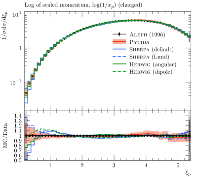
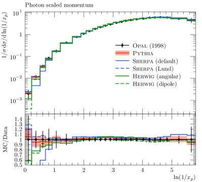
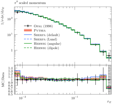
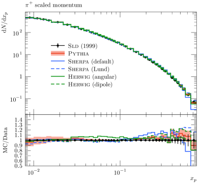
Figure 5: Comparison between MC event generators and LEP and SLD measurements for the log of scaled momentum (top left pane), $\gamma$ spectrum (top right pane), $\pi^{0}$ spectrum (bottom left pane) and $\pi^{\pm}$ spectrum (bottom right pane). Data is taken from Barate:1996fi ; Ackerstaff:1998ap ; Abe:1998zs

In addition to the particle spectra, it is important to ensure that a nonperturbative tuning does not produce “too large” corrections to infrared and collinear safe observables. In the following, we focus on the Thrust and $C$-parameter event shapes as IRC safe controls, which the baseline Monash 2013 tune is known to describe reasonably well Skands:2014pea . (The full set of observables is described in appendix A.) Note that we include the full range of these observables, including also the back-to-back region near $\tau=1-T\to 0$ and $C\to 0$, where the nonperturbative corrections are not power suppressed; this provides a complementary sensitivity to the fragmentation function parameters. Specifically, whereas the particle spectra are only sensitive to the total magnitude of the momentum of the produced hadrons, the nonperturbative corrections to the event shapes are mostly sensitive to the transverse components (the property of IRC safety implies that the correction vanishes for a purely longitudinal breakup), hence they provide important additional sensitivity to the StringPT:sigma parameter in particular.

For completeness and as a cross check on the validity of the often used method of estimating QCD uncertainties by comparing the predictions of different MC generators, we compare several different multi-purpose MC event generators to measurements of the most important observables that we included in the tunes in Figs. 5 and 6. Three event generators are considered in these comparisons; Herwig 7.1.3 Bellm:2015jjp using both the angular-ordered Gieseke:2003rz and dipole Platzer:2009jq ; Platzer:2011bc shower algorithms and a cluster based hadronisation model Webber:1983if , Pythia 8.2.35 with the default model of hadronisation (and using our central tune parameters) Sjostrand:2014zea and Sherpa 2.2.5 Gleisberg:2008ta with the CSS parton shower Schumann:2007mg using both the Ahadic Winter:2003tt (based on the cluster model) and the Pythia 6.4 Lund hadronisation Sjostrand:2006za models. The curve corresponding to Pythia is shown with an uncertainty band (red) obtained using the results of our new tune, based on the recent Monash tune but refitting the three main hadronisation parameters (see below). We can see from Fig. 5 that the multi-purpose event generators agree pretty well except in a few regions;

• In the tails towards hard high-energy fragmentation $\xi=\log(1/x_{\gamma})<1$ (corresponding to $x_{\gamma}\simeq 0.35$ in the bottom-row plots), where a substantial fraction of the energy of the jet is carried by a single particle.

• For very soft photons ($\log(1/x_{p})>4.5$) in the top right-hand plot, the Sherpa curve (corresponding to the Cluster hadronization model) is above all the other predictions (differences are within $5\%$-$10\%$)

• In the momentum of charged pions, Herwig (with the angular shower algorithm) disagrees with the other generators by less than $10\%$ in $0.03<x_{p}<0.1$.

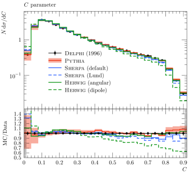
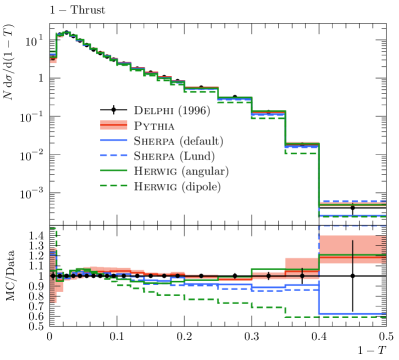
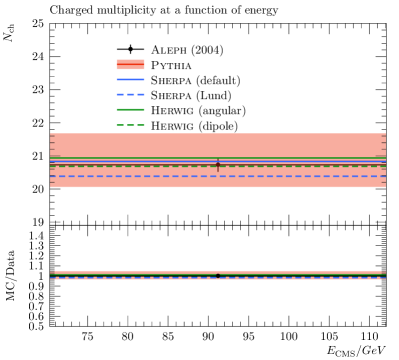
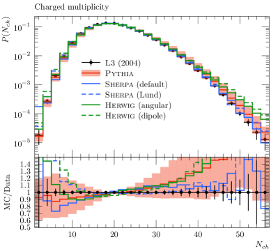
Figure 6: Same as in Fig. 5 but for $C$-parameter (top left pane), $1-T$ (top right pane), mean of charged multiplicity (bottom left pane) and Total charged multiplicity (bottom right pane). Data is taken from Abreu:1996na ; Heister:2003aj ; Achard:2004sv

For the event shapes shown in Fig. 6, the Pythia prediction agrees fairly well with the experimental measurements while there are some tensions with some of the other multi-purpose event generators; e.g. the Herwig dipole shower in the 3-jet regions at large values of the $C$ and $T$ parameters. We conclude that the relative differences between multi-purpose event generators do not faithfully map out the allowed range of uncertainty allowed by data (at least not in the whole spectrum). This finding agrees with the results shown in Cembranos:2013cfa where they find that differences between event generators are more important in the edges and not in the peak region of the photon spectrum. Furthermore, in the context of dark matter searches through $\gamma$-rays, the high $x_{\gamma}$ region of the photon spectrum usually has low statistics and therefore, relative differences between MC event generators, in that region, won’t have a significant impact on the interpretation of the results.

4 Tuning

Pythia8 version 8.235 is used throughout this study. The most recent Monash Skands:2014pea tune is used as baseline for the parameter optimisation (“tuning”). The tuning is performed using Professor v2.2 Buckley:2009bj for the fit to the data, and Rivet v2.5.4 Buckley:2010ar for the implementation of the measurements. The method implemented in Professor permits the simultaneous optimisation of several parameters by using an analytic approximation for the dependence of the physical observables on the model parameters, an idea first introduced in Ref. Abreu:1996na . Polynomials of fourth-order are used to parametrise the response of the observables to the generator parameter. The coefficients in the polynomials are obtained by fitting MC predictions generated at a set of randomly selected parameter points, called anchor points. The optimal values of the model parameters are then obtained with a standard $\chi^{2}$ minimisation of the analytic approximation to the corresponding data using Minuit James:1975dr .

These are the $a$ and $b$ parameters of the Lund fragmentation function ($a$ and $<z_{\rho}>$ in the new parametrization), which govern the longitudinal momentum fractions of produced primary hadrons relative to the jet direction, and the $\sigma$ parameter which governs the transverse components (see e.g. Skands:2012ts ). The default values of the parameters and their allowed range in Pythia8 are shown in Table 1.

To protect against over-fitting effects and as a baseline sanity limit for the achievable accuracy in both the perturbative and nonperturbative modeling regimes, we introduce an additional $5\%$ uncertainty on each bin and for each observable. This also substantially reduces the value of the goodness-of-fit measure so that the resulting $\chi^{2}/\textrm{ndf}$ is consistent with unity (see Table 2). The absence of such an additional uncertainty in the tune leads to an overconstrained fit with a large central $\chi^{2}$ value and artificially small parameter variations which cannot be interpreted as conservative estimate of the uncertainty. The MC statistical uncertainties are treated as uncorrelated and included in the definition of the $\chi^{2}$ function, which thus becomes:

$$\frac{\chi^{2}}{N_{\textrm{DoF}}}=\frac{1}{\sum_{\mathcal{O}}\omega_{\mathcal{O}}|b\in\mathcal{O}|}\frac{\sum_{\mathcal{O}}\omega_{\mathcal{O}}\sum_{b\in\mathcal{O}}(f_{(b)}(\textbf{p})-\mathcal{R}_{b})^{2}}{(\Delta_{b}^{2}+(0.05f_{(b)}(\textbf{p}))^{2})}~{}.$$ (5)

Here $\omega_{\mathcal{O}}$ represents the weight per observable and per bin, $f_{(b)}(\textbf{p})$ is the interpolation function per bin $b$, $\mathcal{R}_{b}$ is the experimental value of the observable $\mathcal{O}$ and $\Delta_{b}$ is the experimental error per bin. A fourth-order polynomial was used as interpolating function $f_{(b)}$. We have checked the robustness of the interpolations by comparing the response functions to the real generated runs at the minimum and found excellent agreement. To get a good tune, we have to use a large number of MC runs. For this study, 120 random combinations of 1000 independent runs, with 2M events for each, have been used.

parameter	Pythia8 setting	Variation range	Monash
$\sigma_{\perp}$ [GeV]	StringPT:Sigma	0.0 – 1.0	0.335
$a$	StringZ:aLund	0.0 – 2.0	0.68
$b$	StringZ:bLund	0.2 – 2.0	0.98
$\left<z_{\rho}\right>$	StringZ:avgZLund	0.3 – 0.7	(0.55)

Table 1: Parameter ranges used for the Pythia 8 tuning, and their corresponding value in the Monash tune. The parenthesis around the Monash value of the $\left<z_{\rho}\right>$ parameter indicates that this is a derived quantity, not an independent parameter.

As a first step in the tuning to the $e^{+}e^{-}$ measurements, a study of the sensitivity of the various observables to the MC parameters is performed. The results of the sensitivity study is used to guide the selection of the observables to use for tuning. The sensitivity of each observable bin to a set of parameters $p_{i}$, is estimated from the interpolated response of the observables to the parameters, with the following formula:

$$\mathcal{S}_{i}=\frac{\partial\mathrm{MC}(p)}{|\mathrm{MC}(p_{0})|+\epsilon w_{\rm MC}}\frac{|p_{0,i}|+\epsilon w_{p_{i}}}{\partial p_{i}},$$ (6)

where $p_{0}$ is the centre of the parameters range, MC$(p_{0})$ is the interpolated MC prediction at $p_{0}$ and the $\epsilon$ terms, set to 1% of the parameter range, are introduced to avoid the ill defined case MC$(p_{0})=0$, $\partial p_{i}=0$. $w_{p_{i}}$ corresponds to 80% of the original sampling range and is used to construct $w_{\rm MC}$.

The sensitivity of different observables to the Lund fragmentation function parameters’ is shown in Figs. 7 and 8. The observables are selected from different measurements and corresponding to the charged multiplicity, log of scaled momentum, spectra of charged pions, neutral pions, photons and $\eta$-mesons, the Thrust and the $C$-parameter. As we can see from Figs. 7-8, all the observables are sensitive to the variations of the parameters notably to avgZLund.

We tune the parameters of the string fragmentation function in Pythia 8 to a set of sensitive Lep and Slc measurements at the $Z$-boson peak produced by Aleph Decamp:1991uz ; Buskulic:1992hn ; Buskulic:1995au ; Barate:1996fi ; Barate:1996uh ; Heister:2001kp ; Heister:2003aj , Delphi Abreu:1990cc ; Adam:1995rf ; Abreu:1996na , L3 Adeva:1991it ; Adriani:1992hd ; Acciarri:1994gza ; Achard:2004sv , Opal Akers:1994ez ; Ackerstaff:1998ap ; Ackerstaff:1998hz ; Abbiendi:2004qz and Sld Abe:1996zi ; Abe:1998zs ; Abe:2003iy . Several qualitatively different tunes are made, by including or excluding different data sets (and/or by modifying their weights). Our first tune, labeled T1, only includes the spectra of $\pi^{0,\pm},\gamma$ and $\eta$ particles. A second tune, labeled T2, also includes event-shapes and jet-rate observables, and hence represents a more global fit. The weights assigned to each measurement in these two tunes are colled in Tables 9-14. Further, to access to the compatibility between the different experiments, we tune to each experiment individually including all the aforementioned observables with unit weights. The resulting five independent tunes are labeled by the names of the corresponding experiments.

At the technical level, we set up the event generation for an incoming $e^{+}e^{-}$ pair with QED initial-state effects switched off. (This corresponds to the definition of the unfolded experimental measurements used in the tuning.) We adopted the same definition of particle stability as it was used by LEP, i.e a given particle is stable if its mean lifetime satisfies $c\tau_{0}>100$ mm. Finally, the strong coupling constant for Final State Radiation (FSR) was set to be $\alpha_{S}(M_{Z}^{2})=0.1365$ with a one-loop running as in the Monash tune. All the other parameters and settings in Pythia are fixed to their default values. The specific commands used in the tuning setup are shown in appendix C.

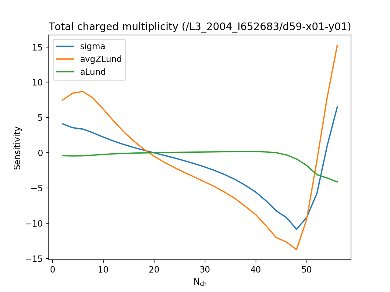
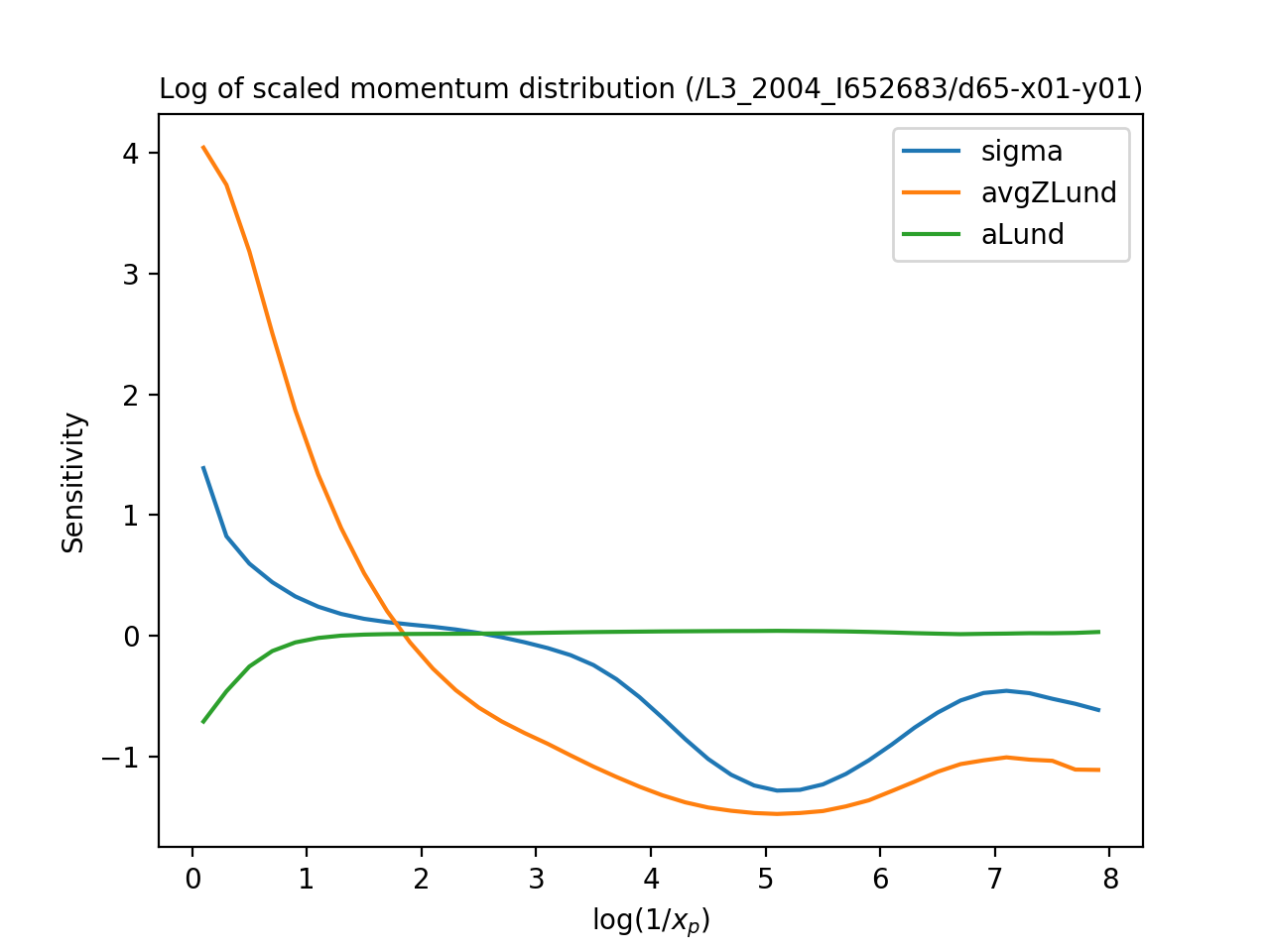
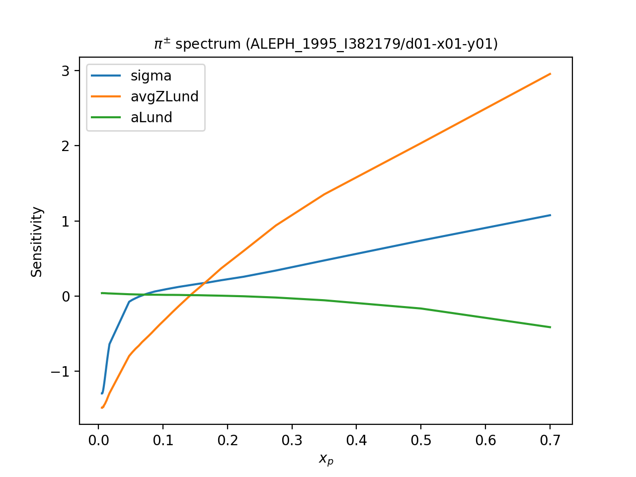
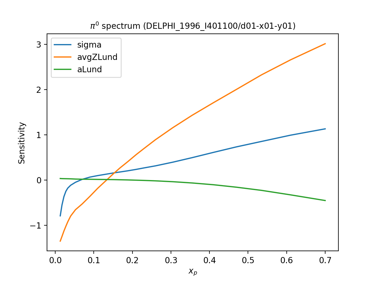
Figure 7: Sensitivity of the different observables to the Pythia 8 fragmentation parameters $\sigma_{\perp}$ (blue), $\left<z_{\rho}\right>$ (orange), $a$ (green). The sensitivities are shown as functions of the charged particle multiplicity $N_{\rm ch}$ (a), the total scaled momentum $x_{p}$ (b), the $\pi^{\pm}$ scaled momentum (c), and the $\pi^{0}$ scaled momentum (d).

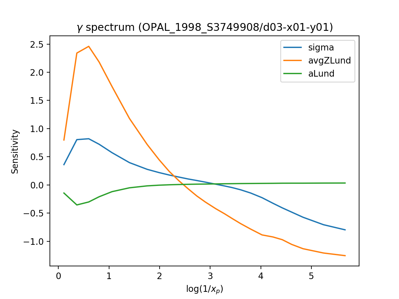
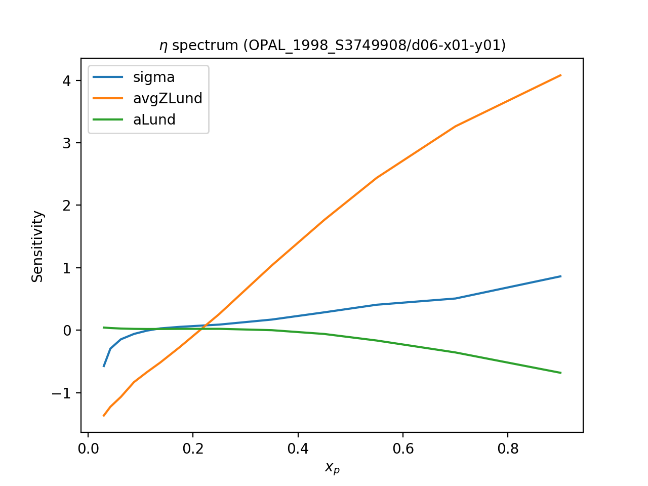
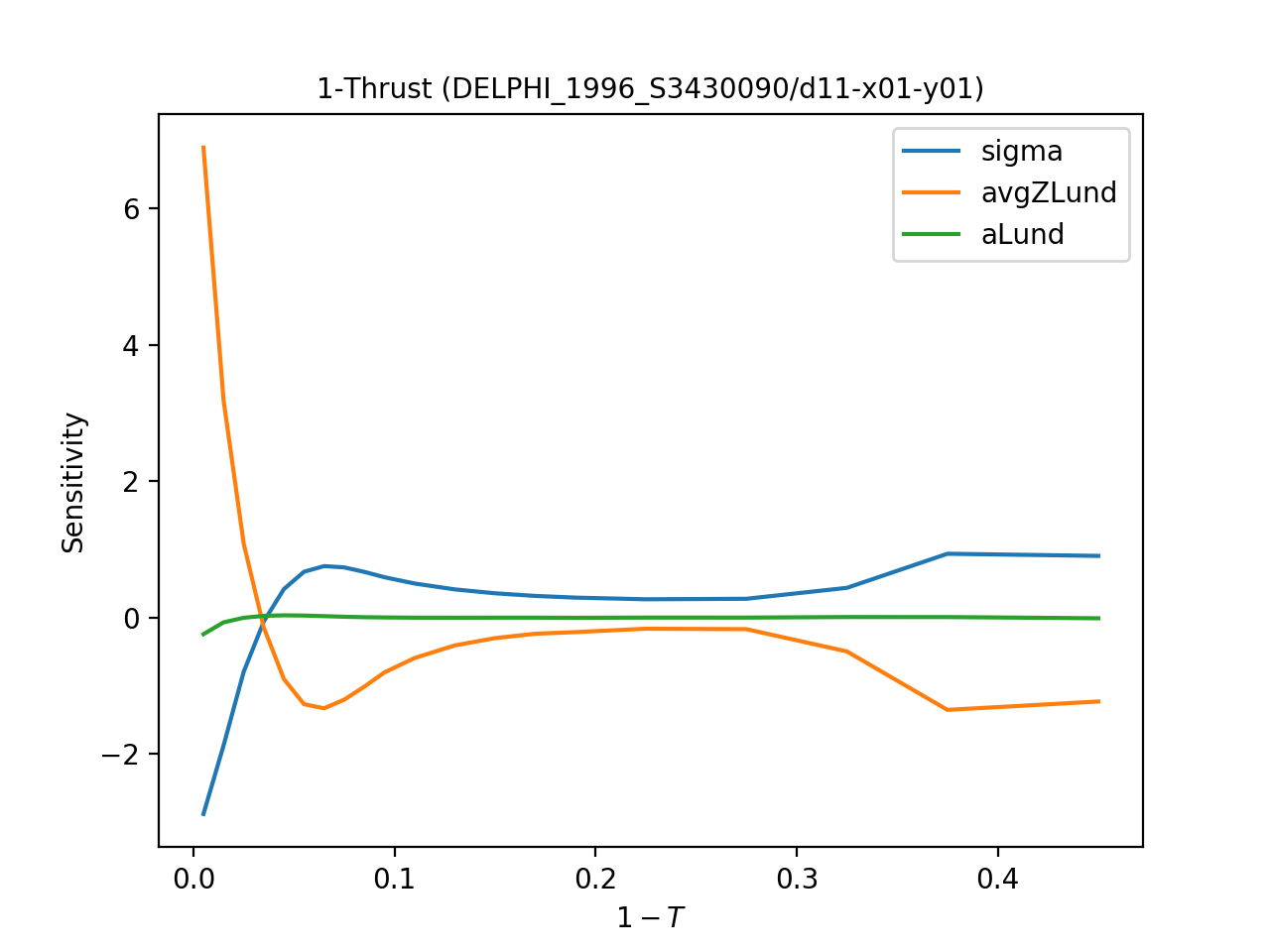
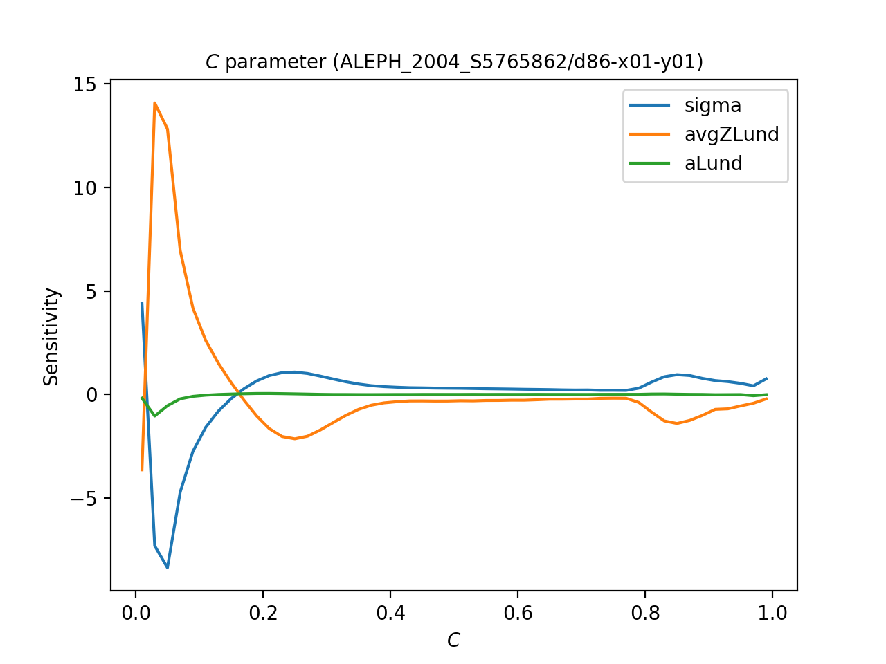
Figure 8: Same as in Fig. 7 but for the $\gamma$ scaled momentum (a), the $\eta$ scaled momentum (b), the Thrust distribution (c) and the $C$-parameter distribution (d).

5 Results

In this section, we present results of our tunes and related uncertainties. We compare two different methods: eigentunes and manual variations of parameters. We find that the eigentune method does not provide acceptably conservative uncertainty estimates and therefore advocate for a more elaborate method which we describe in section 5.2.

5.1 Tunes

We start by discussing the correlation among the parameters in the two parameterizations of the Lund fragmentation function. To illustrate this, we show in Fig. 9, the correlation matrix $C_{ij}$ obtained from the T2 tune in the old (left) and the new (right) parameterizations of the Lund fragmentation function. Clearly StringZ:aLund and StringZ:bLund are highly correlated ($C_{12}=89\%$). Using the new parametrization reduces the correlation by about $13\%$ where now the StringZ:bLund is replaced by StringZ:avgZLund. Furthermore, we note that the remaining correlation is almost entirely associated with the mean multiplicities. If these are removed from the fit, the strong correlation between StringZ:aLund and StringZ:avgZLund is considerably reduced. Furthermore, in the old parametrization, StringZ:aLund and StringPT:sigma have a correlation coefficient of $44\%$ which is reduced to $-9\%$ in the new parametrization of the Lund function.

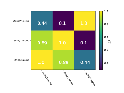
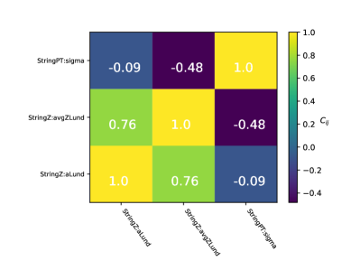
Figure 9: The parameters correlation ($C_{ij}$) as evaluated from the Hessian matrix at the fit minimum. (a) shows result with standard parametrization of the Lund string in terms of the $a$, $b$ parameters, (b) results with a new parametrization in terms of the $a$ and $<z_{\rho}>$ parameters.

Since these are just two different parametrisations of the same function, it is interesting to check whether one gets compatible values for the tune parameters when fitting the two different forms to the same data. For this purpose, we make a comparison between the two parameterizations showing, as an example, the T2 tune. We show the results of this comparison in the (StringPT:sigma, StringZ:aLund) plane in Fig. 10. While it looks obvious from Fig. 10 that the two tunes give inconsistent results even at the $3\sigma$ level, the two tunes are in good agreement with each other on data as can be seen in Fig. 11 (the same conclusion applies for all the other measurements which are not shown here). This can explained via the correlation with the remaining parameter, $b$: while the two tunes gives very different central values for StringZ:aLund and StringPT:sigma, the obtained value for StringZ:bLund is also different. This is a clear reminder that misleading conclusions can be reached if correlations are neglected.

As pointed out in the previous section, including the $5\%$ theory uncertainty affects significantly the quality of the tune. This is can be seen in Table 2, where the results of the tune before and after including the $5\%$ uncertainty are compared. While the resulting parameters are consistent in the two fits, the goodness-of-fit per degree of freedom is improved by a factor of $~{}7$, bringing it close to unity for the second fit. The uncertainties on the parameter’s determination are also affected, being significantly larger when the additional 5% uncertainty is added to the fit. We therefore consider that the added $5\%$ uncertainty does provide a useful basic protection against overfitting, and prefer the more conservative uncertainties this way, being consistent with a $\Delta\chi^{2}\pm 1$ around a central $\chi^{2}$ of order unity.

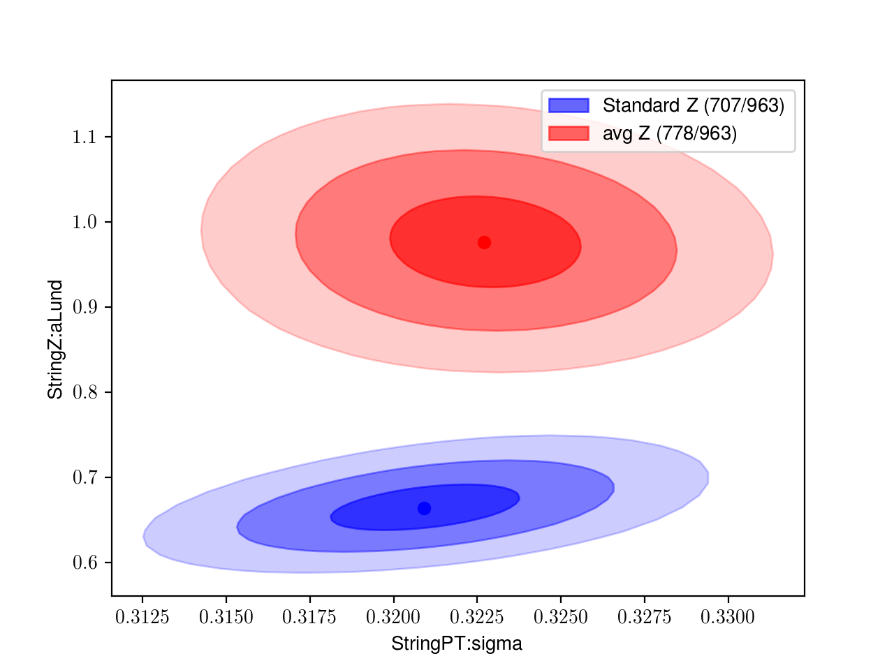
Figure 10: Results of tunes using the standard parametrization of the Lund string (blue) in terms of the $a$, $b$ parameters, and with a new parametrization (red) in terms of the $a$ and $\left<z_{\rho}\right>$ parameters.

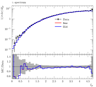
Figure 11: Comparison between the results of the tune in the old (StandardZ) and the new (AvgZ) parametrization of the Lund fragmentation function for scaled momentum distribution of charged particles (left) and photon scaled momentum (right). Data is taken from Barate:1996fi .

Parameter	without $5\%$	with $5\%$
StringPT:Sigma	$0.3151\begin{subarray}{c}+0.0010\\ -0.00010\end{subarray}$	$0.3227\begin{subarray}{c}+0.0028\\ -0.0028\end{subarray}$
StringZ:aLund	$1.028\begin{subarray}{c}+0.031\\ -0.031\end{subarray}$	$0.976\begin{subarray}{c}+0.054\\ -0.052\end{subarray}$
StringZ:avgZLund	$0.5534\begin{subarray}{c}+0.0010\\ -0.0010\end{subarray}$	$0.5496\begin{subarray}{c}+0.0026\\ -0.0026\end{subarray}$
$\chi^{2}$/ndf	5169/963	778/963

Table 2: Results of tunes using the new parametrization of the Lund fragmentation function in terms of the $a$ and $\left<z_{\rho}\right>$ parameters. The second (third) column shows the result before (after) including a flat $5\%$ uncertainty to the theory prediction.

Tune	StringZ:aLund	StringZ:avgZLund	StringPT:sigma	$\chi^{2}$/ndf
Aleph	$0.827\begin{subarray}{c}+0.066\\ -0.062\end{subarray}$	$0.5447\begin{subarray}{c}+0.0044\\ -0.0044\end{subarray}$	$0.3105\begin{subarray}{c}+0.0045\\ -0.0045\end{subarray}$	284.7/382
Delphi	$0.67\begin{subarray}{c}+0.11\\ -0.09\end{subarray}$	$0.5290\begin{subarray}{c}+0.0062\\ -0.0063\end{subarray}$	$0.3110\begin{subarray}{c}+0.0062\\ -0.0061\end{subarray}$	82/113
L3	$1.186\begin{subarray}{c}+0.093\\ -0.10\end{subarray}$	$0.5708\begin{subarray}{c}+0.0054\\ -0.0055\end{subarray}$	$0.3303\begin{subarray}{c}+0.0072\\ -0.0072\end{subarray}$	98/155
Opal	$0.55\begin{subarray}{c}+0.11\\ -0.095\end{subarray}$	$0.511\begin{subarray}{c}+0.011\\ -0.012\end{subarray}$	$0.318\begin{subarray}{c}+0.013\\ -0.013\end{subarray}$	82.4/184
Sld	$0.95\begin{subarray}{c}+0.12\\ -0.11\end{subarray}$	$0.5271\begin{subarray}{c}+0.0097\\ -0.010\end{subarray}$	$0.327\begin{subarray}{c}+0.017\\ -0.017\end{subarray}$	34.4/116
COMBINED	$0.976\begin{subarray}{c}+0.054\\ -0.052\end{subarray}$	$0.5496\begin{subarray}{c}+0.0026\\ -0.0026\end{subarray}$	$0.3227\begin{subarray}{c}+0.0028\\ -0.0028\end{subarray}$	778/963

Table 3: Results of the tunes performed separately to all the considered measurements from a given experiment. The COMBINED result corresponds to the T2 tune given in Table 2.

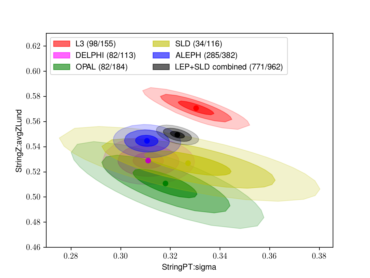
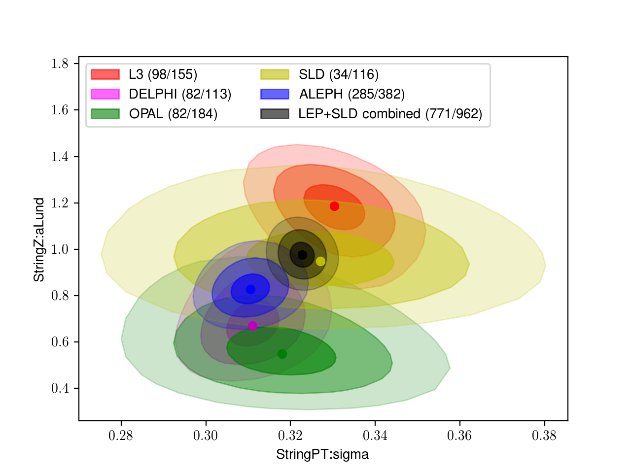
Figure 12: Results of tunes performed separately to all of the measurements from a given experiment; Aleph (blue), Delphi (magenta), L3 (red), Opal (green), Sld (yellow) and COMBINED (gray). The contours corresponding to one, two and three sigma deviations are also shown.

We now turn to a study of possible tensions in the data measured by the different experiments by making independent tunes including all of the sensitive measurements by each experiment. Five independent tunes are performed corresponding to the data measured by Aleph, Delphi, L3, Opal and Sld. The results of these tunes are shown in figure 12 and Table 3. We can see that the tunes to Aleph, Delphi, Opal and Sld are in agreement regarding the obtained value of StringZ:avgZLund contrarily to L3. Again, due to the correlations of $a$ with $b$ (or $<z_{\rho}$), we cannot conclude anything from comparisons of each individual parameters and, therefore, when compared on data, various tunes are expected to be in good agreement with each other.

Tune	StringZ:aLund	StringZ:avgZLund	StringPT:sigma	$\chi^{2}$/ndf
Charged multiplicity	$1.061\begin{subarray}{c}+0.089\\ -0.096\end{subarray}$	$0.518\begin{subarray}{c}+0.011\\ -0.012\end{subarray}$	$0.410\begin{subarray}{c}+0.017\\ -0.016\end{subarray}$	43.4/104
Scaled momentum	$0.598\begin{subarray}{c}+0.053\\ -0.049\end{subarray}$	$0.5295\begin{subarray}{c}+0.0070\\ -0.0072\end{subarray}$	$0.324\begin{subarray}{c}+0.012\\ -0.012\end{subarray}$	70.7/180
$\gamma$	$0.61\begin{subarray}{c}+0.32\\ -0.23\end{subarray}$	$0.517\begin{subarray}{c}+0.035\\ -0.039\end{subarray}$	$0.344\begin{subarray}{c}+0.067\\ -0.062\end{subarray}$	52.4/70
$\pi^{0}$	$1.22\begin{subarray}{c}+0.18\\ -0.16\end{subarray}$	$0.566\begin{subarray}{c}+0.014\\ -0.014\end{subarray}$	$0.340\begin{subarray}{c}+0.020\\ -0.020\end{subarray}$	31/117
$\pi^{\pm}$	$0.757\begin{subarray}{c}+0.082\\ -0.073\end{subarray}$	$0.5029\begin{subarray}{c}0.0098\\ -0.0099\end{subarray}$	$0.336\begin{subarray}{c}+0.011\\ -0.011\end{subarray}$	72.5/205
$T$	$1.34\begin{subarray}{c}+0.27\\ -0.20\end{subarray}$	$0.498\begin{subarray}{c}+0.018\\ -0.019\end{subarray}$	$0.241\begin{subarray}{c}+0.022\\ -0.023\end{subarray}$	124/194
$C$-parameter	$1.65\begin{subarray}{c}+0.35\\ -0.42\end{subarray}$	$0.621\begin{subarray}{c}+0.053\\ 0.038\end{subarray}$	$0.390\begin{subarray}{c}+0.067\\ -0.043\end{subarray}$	23.4/71
$\gamma,\pi^{0,\pm}$ (T1)	$0.821\begin{subarray}{c}0.065\\ -0.060\end{subarray}$	$0.5291\begin{subarray}{c}+0.0057\\ -0.0057\end{subarray}$	$0.3304\begin{subarray}{c}+0.0060\\ -0.0060\end{subarray}$	321/514
All (T2)	$0.976\begin{subarray}{c}+0.054\\ -0.052\end{subarray}$	$0.5496\begin{subarray}{c}+0.0026\\ -0.0026\end{subarray}$	$0.3227\begin{subarray}{c}+0.0028\\ -0.0028\end{subarray}$	778/963

Table 4: Results of tunes performed separately to measurements of charged multiplicity, charged scaled momentum, $\gamma$ spectra, $\pi^{0}$ spectra, $\pi^{\pm}$ spectra, Thrust distribution and $C$-parameter. Results of tunes combining measurements of $\gamma$,$\pi^{\pm}$ and $\pi^{0}$ (T1) or all measurements (T2) are also reported.

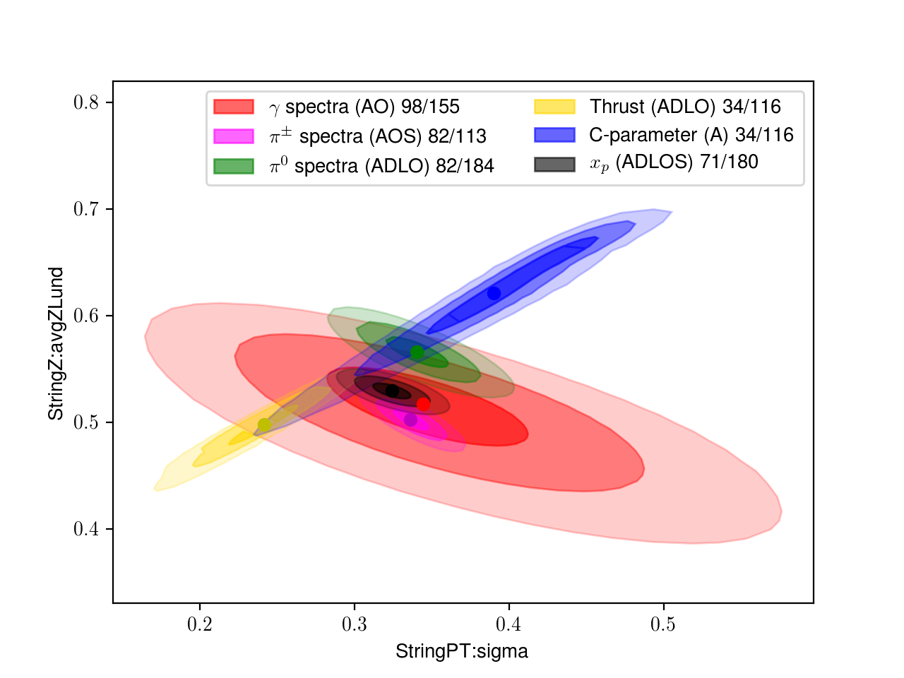
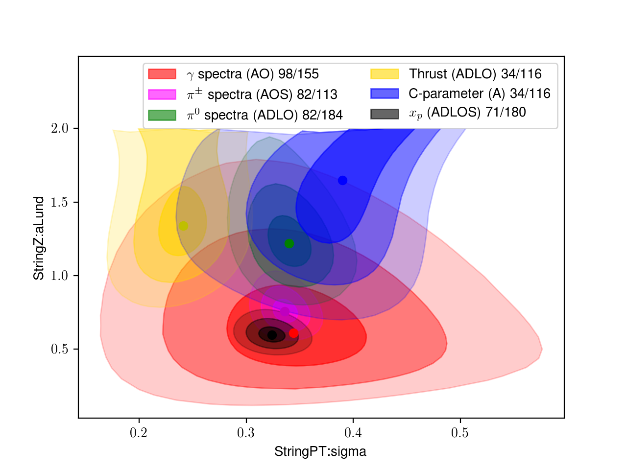
Figure 13: Results of tunes performed separately to measurements of $\gamma$ spectra (red), $\pi^{\pm}$ spectra (magenta), $\pi^{\pm}$ spectra (green), Thrust distribution (yellow), $C$-parameter (blue) and charged particles scaled momentum (black). Measurements from Aleph (A), Delphi (D), Opal (O), L3 (L) and Sld (S) are used. The contours corresponding to a one, two and three standard deviations are also shown.

Tuning the same observable from different experiments is very important to assess the constraining power of a given observable and to validate sensitivity studies which were carried in section 4. The results of these fits are depicted in Fig. 13 and Table 4. In this part of the tuning, we focused on charged multiplicity, $\gamma$, $\pi^{0}$, $\pi^{\pm}$, and charged particles’ spectra, $C$-parameter and the Thrust distribution. We, first, observe that the obtained value of StringZ:aLund from the tuning to the $C$ and $T$ parameters is not consistent at all either with the well established Monash tune or with the other results. This is an expected result given the fact that the $C$ and $T$ parameters have less sensitivity (expect in their first few bins) on the fragmentation model and they are mainly sensitive to the shower parameters, which are not varied in this study. Furthermore, for the same observables, the StringZ:avgZLund and StringPT:sigma parameters are highly correlated as can be seen from Fig. 13.

Variation	StringZ:aLund	StringZ:avgZLund	StringPT:sigma
Central	0.9757	0.5496	0.3227
OneUp	0.9233	0.5476	0.3230
OneDw	1.0300	0.5516	0.3225
TwoUp	0.9757	0.5509	0.3200
TwoDw	0.9758	0.5483	0.3255
ThreeUp	0.9757	0.5507	0.3233
ThreeDw	0.9758	0.5485	0.3222

Table 5: The Hessian variations (eigentunes) for the nominal tune including all observables corresponding to a one standard deviation (68% CL) interval.

Parameter	Value
StringZ:aLund	$0.5999\pm 0.2$
StringZ:avgZLund	$0.5278^{+0.027}_{-0.023}$
StringPT:sigma	$0.3174^{+0.042}_{-0.037}$

Table 6: Result of the single fit to all the measurements as obtained from Fig. 14. The quoted errors correspond to the $68\%$ CL uncertainty on the fit.

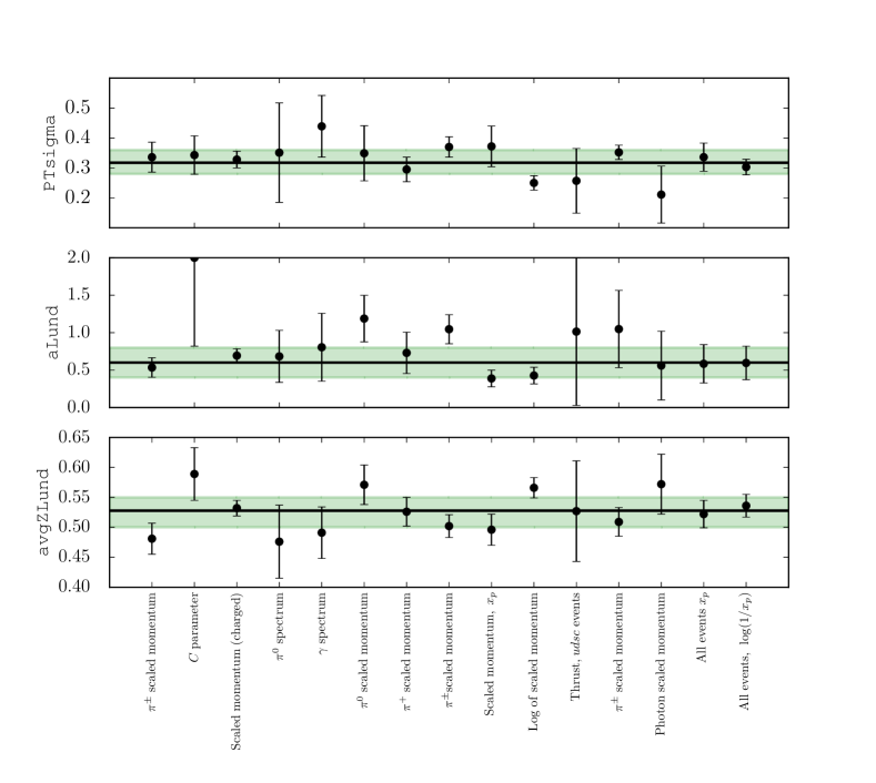
Figure 14: Results of tunes performed separately to each of the observables. The weighted average of the tunes to the individual measurements is shown with a black line. A green shaded area indicated the 68% CL interval on the parameters.

5.2 Uncertainties

After discussing in details the results of the tuning and independent fits, we move to the question of QCD uncertainties. Those can be separated into the perturbative uncertainties, related to the parton showers evolution, and the non-perturbative ones, related to the determination of the parameters of the fragmentation model. Uncertainties on the non-perturbative part, are specific to the chosen model and the data used to constrain them, leaving more ambiguities in the uncertainty estimate.

Uncertainties on parton showering in Pythia8 are estimated using the automatic setup developed in (Mrenna:2016sih, ) which aims for a comprehensive uncertainty bands by variation the central renormalization scale by a factor of $2$ in the two directions with a full NLO scale compensation. Such perturbative uncertainties are investigated independently from those on the parameters of the Lund fragmentation function. Furthermore, the framework also allows for variations of non-singular terms in the Dokshitzer-Gribov-Lipatov-Altarelli-Parisi (DGLAP) splitting kernels as an additional, complementary handle on the perturbative uncertainties (the singular part of the DGLAP functions is universal while non-singular terms can be used to represent potential effects of process dependence). In most of the cases, variations of the non-singular terms give small uncertainties ($\simeq 1\%$) and can safely be neglected.

On the non-perturbative side, two methods are employed to obtain uncertainties on the parameters of the Lund fragmentation function. The Professor toolkit allows to estimate uncertainties on the fitted parameters through the eigentunes method. This method diagonalises the $\chi^{2}$ covariance matrix around the best fit point, and uses variations along the principal directions (eigenvectors) in the space of the optimised parameters to build a set of $2\cdot N_{\textrm{params}}$ variations. Variations are obtained moving along the eigenvectors for direction corresponding to a fixed change in the goodness-of-fit (GoF) measure. If the GoF measure follows a $\chi^{2}$ statistics, one can define the $\Delta\chi^{2}$ corresponding to a given confidence level interval. However, due to the intrinsic limitations of the phenomenological models used in event generators and the lack of correlation in systematic uncertainties between observables and bins in the tunes, this is usually not the case. Heuristic choices of $\Delta\chi^{2}$ are typically chosen in tunes to obtain a reasonable coverage of the uncertainties in the experimental data. In our study this is obtained by the addition of a 5% uncertainty to the MC predictions, allowing for $\chi^{2}$/NDoF of order one in our tunes. The resulting eigentunes are however still found to provide small uncertainties which cannot be interpreted as conservative. The uncertainty on the parameters of the Lund fragmentation function are very small (below the one percent level) and inconsistent with the uncertainties of the data used in the tune. In Table 7 we also show the uncertainties from QCD on the photon spectra in the peak region for $\chi\chi\to gg$ for $m_{\chi}=25$ GeV where the nominal values of the parameters correspond to the result of T2 tune and the corresponding eigentunes are shown in Table 5.

Therefore, we use an alternative method to estimate the uncertainty on the Lund fragmentation function’s parameters. We, first, make a fit each measurement. Thus, for $N$ measurements, we get $N$ best-fit points for each parameter. We then take the $68\%$ CL errors on the parameters to be our estimate of the uncertainty taking care to exclude observables with little or no sensitivity to the given parameters. The results of these fits along with their $68\%$ CL errors are shown in both Fig. 14 and Table 6. We checked, that the predictions of this single fit agree fairly well with the T2 tune. We discuss how to obtain comprehensive uncertainty bands from the $68\%~{}\textrm{CL}$ errors on the parameter. We denote a variation on the parameters $\verb|(StringPT:sigma, StringZ:avgZLund, StringZ:aLund)|\equiv(\sigma,z_{\rho},a)$ by $(X_{1},X_{2},X_{3})$ with $X_{i}=+,-,0$. The $+$($-$) corresponds to a variation of the parameter $X_{i}$ in the positive (negative) direction with respect to the nominal value denoted by $0$. Besides the nominal tune corresponding to $(0,0,0)$, there are $3^{3}-1=26$ possible variations. However, there are some variations which don’t give observable effects on the spectra and, therefore, can be neglected. To understand this, we discuss the effects of different parameters on the most significant observables, i.e the event shapes and scaled momenta. If one increases $\sigma$, we get few hard hadrons because if a particle takes more mean transverse momentum $<p_{T}>$ then there will be no enough phase space for the other hadrons. On the other hand, decreasing $\sigma$ will result in many low $p_{T}$ hadrons. The effect of $z_{\rho}$ is similar to $\sigma$ but on the total momentum. The $a$ parameter has a similar effect on the particle momenta but with an reversed behavior in a sense that if $z_{\rho}$ and $a$ are varied in the same direction, their effect will almost compensate and therefore one gets no bands in the high energy bins. The same $a$ parameter has no effect on the event shapes as $\sigma$ and $z_{\rho}$ do. We stress finally that varying $\sigma$, and $z_{\rho}$ in opposite directions has large effect on the lowest bins of the event shapes (Thrust for example). Hence, the $(+,-,X)$ and $(-,+,X)$ have the most significant effects on the event shapes. In conclusion, the envelope that we consider as a faithful representation of the QCD uncertainty is obtained from $10$ variations; $(+,+,0),(-,-,0),(+,+,+),(-,-,-),(+,-,+),(+,-,-),(-,+,+),(-,+,-),(-,+,0)$ and $(+,-,0)$ in addition to the nominal one. Their effects are shown in Figs. 5 and 6 and used in the impact on DM fits. Furthermore, the updated tables for particle spectra will be provided with their uncertainties (obtained from these variations and from shower uncertainties as well).

$x_{\gamma}$	$(\textrm{d}N/\textrm{d}x_{\gamma})_{\texttt{T2}}\pm\delta_{\textrm{had.}}\pm\delta_{\textrm{shower}}$
$0.00125$	$7.59\begin{subarray}{c}+0.05\%\\ -0.0\%\end{subarray}\begin{subarray}{c}+8.1\%\\ -4.8\%\end{subarray}$
$0.002$	$13.79\begin{subarray}{c}+0.18\%\\ -0.26\%\end{subarray}\begin{subarray}{c}+8.3\%\\ -4.9\%\end{subarray}$
$0.003$	$22.29\begin{subarray}{c}+0.13\%\\ -0.0\%\end{subarray}\begin{subarray}{c}+8.2\%\\ -4.9\%\end{subarray}$
$0.005$	$31.95\begin{subarray}{c}+0.2\%\\ -0.04\%\end{subarray}\begin{subarray}{c}+8.1\%\\ -4.8\%\end{subarray}$
$0.008$	$40.74\begin{subarray}{c}+0.12\%\\ -0.05\%\end{subarray}\begin{subarray}{c}+7.7\%\\ -4.6\%\end{subarray}$
$0.0125$	$45.83\begin{subarray}{c}+0.08\%\\ -0.09\end{subarray}\begin{subarray}{c}+7.1\%\\ -4.3\%\end{subarray}$
$0.02$	$45.01\begin{subarray}{c}+0.13\%\\ -0.02\end{subarray}\begin{subarray}{c}+6.5\%\\ -4.0\%\end{subarray}$
$0.03$	$39.43\begin{subarray}{c}+0.13\%\\ -0.0\%\end{subarray}\begin{subarray}{c}+5.2\%\\ -3.3\%\end{subarray}$
$0.05$	$30.73\begin{subarray}{c}+0.0\%\\ -0.15\%\end{subarray}\begin{subarray}{c}+3.1\%\\ -2.1\%\end{subarray}$
$0.08$	$21.36\begin{subarray}{c}+0.0\%\\ -0.06\%\end{subarray}\begin{subarray}{c}+0.4\%\\ -0.5\%\end{subarray}$
$0.125$	$12.98\begin{subarray}{c}+0.13\%\\ -0.23\%\end{subarray}\begin{subarray}{c}+1.6\%\\ -3.0\%\end{subarray}$

Table 7: Scaled momentum of photons in the process $\chi\chi\to gg$ for $m_{\chi}=25$ GeV where only the peak region of the spectra is shown. In this table, we show the predictions from the weighted tune denoted by T2 (the central values of the parameters and their eigentunes are shown in Tables 2 and 5). The $68\%$ CL on hadronisation parameters are shown as first errors for each bin while uncertainties due to shower variations are the second errors.

$E_{\gamma}$ [GeV]	Hadronization	Shower	Herwig	Total
$0.4$	${}^{+6.17\%}_{-5.57\%}$	${}^{+8.24\%}_{-4.91}$	$-21.31\%$	${}^{+10.29\%}_{-22.56\%}$
$1.2$	${}^{+2.57\%}_{-2.47\%}$	${}^{+5.94\%}_{-3.68}$	$-6.57\%$	${}^{+6.47\%}_{-7.92\%}$
$2.0$	.${}^{+1.23\%}_{-1.28\%}$	${}^{+3.51\%}_{-2.24\%}$	$-1.51\%$	${}^{+3.71\%}_{-2.98\%}$
$2.8$	${}^{+0.70\%}_{-0.69\%}$	${}^{+1.78\%}_{-1.18\%}$	$-0.39\%$	${}^{+1.91\%}_{-2.34\%}$
$3.6$	${}^{+0.42\%}_{-1.03\%}$	${}^{+0.10\%}_{-0.15\%}$	$-0.31\%$	${}^{+0.43\%}_{-1.08\%}$
$4.4$	${}^{+1.08\%}_{-1.21\%}$	${}^{+0.68\%}_{-1.24\%}$	$-0.70\%$	${}^{+1.27\%}_{-2.14\%}$
$5.2$	${}^{+1.43\%}_{-1.63\%}$	${}^{+1.40\%}_{-2.46\%}$	$-0.97\%$	${}^{+2.00\%}_{-3.10\%}$
$6.0$	${}^{+1.84\%}_{-1.97\%}$	${}^{+2.09\%}_{-3.88\%}$	$-1.60\%$	${}^{+2.78\%}_{-4.63\%}$
$6.8$	${}^{+2.14\%}_{-2.33\%}$	${}^{+2.60\%}_{-4.56\%}$	$-1.61\%$	${}^{+3.36\%}_{-5.36\%}$
$7.6$	${}^{+2.86\%}_{-2.56\%}$	${}^{+3.02\%}_{-4.96\%}$	$-1.51\%$	${}^{+4.15\%}_{-5.78\%}$
$8.4$	${}^{+3.28\%}_{-3.04\%}$	${}^{+3.72\%}_{-5.97\%}$	$-1.40\%$	${}^{+4.95\%}_{-6.84\%}$
$9.2$	${}^{+2.72\%}_{-4.05\%}$	${}^{+4.10\%}_{-6.54\%}$	$-2.20\%$	${}^{+4.92\%}_{-8.00\%}$
$10$	${}^{+3.55\%}_{-4.12\%}$	${}^{+4.13\%}_{-6.73\%}$	$-2.04\%$	${}^{+5.44\%}_{-8.15\%}$
$14$	${}^{+4.34\%}_{-4.35\%}$	${}^{+6.30\%}_{-9.58\%}$	$-1.44\%$	${}^{+7.65\%}_{-10.62\%}$
$18$	${}^{+5.90\%}_{-4.99\%}$	${}^{+6.88\%}_{-10.58\%}$	$+0.76\%$	${}^{+9.09\%}_{-11.69\%}$
$22$	${}^{+4.15\%}_{-4.27\%}$	${}^{+7.58\%}_{-11.99\%}$	$+0.88\%$	${}^{+8.68\%}_{-12.72\%}$
$30$	${}^{+5.50\%}_{-5.18\%}$	${}^{+9.76\%}_{-8.91\%}$	$+2.41\%$	${}^{+11.45\%}_{-10.30\%}$
$38$	${}^{+6.77\%}_{-11.04\%}$	${}^{+8.97\%}_{-14.17\%}$	$-5.49\%$	${}^{+11.23\%}_{-18.78\%}$
$42$	${}^{+0.54\%}_{-10.74\%}$	${}^{+11.82\%}_{-8.57\%}$	$-15.15\%$	${}^{+11.83\%}_{-20.45\%}$
$52$	${}^{+25.19\%}_{-22.96\%}$	${}^{+5.75\%}_{-12.29\%}$	$-8.71\%$	${}^{+25.83\%}_{-27.46\%}$
$64$	${}^{+13.33\%}_{-53.33\%}$	${}^{+0.0\%}_{-9.25\%}$	$-46.81\%$	${}^{+13.33\%}_{-71.56\%}$

Table 8: Uncertainties on the photon spectra in the region ($0.4~{}$GeV $\leq E_{\gamma}\leq 64$ GeV for $W^{+}W^{-}$ annihilation channel of DM corresponding to $m_{\chi}=90.6$ GeV. We show hadronization uncertainties, shower uncertainties and uncertainties from the relative difference between Herwig and Pythia. Total uncertainties are shown by summing in quadrature.

5.3 Impact on Dark Matter Spectra and Fits

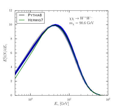
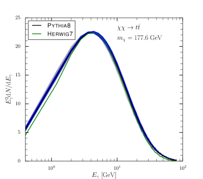
Figure 15: Photon energy distribution for dark matter annihilation into $W^{+}W^{-}$ with $m_{\chi}=90.6$ GeV (left) and into $t\bar{t}$ with $m_{\chi}=177.6$ GeV (right). In the two cases, the result corresponding to the new tune is shown in black line. Both the uncertainties from parton showering (gray bands) and from hadronisation (blue bands) are shown. Predictions from Herwig7 are shown as a gray solid line.

In this subsection, we study the impact of QCD fragmentation function, parton shower and MC event generators uncertainties on the photon spectra of two representative DM annihilation channels: $W^{+}W^{-}$ and $t\bar{t}$. Our motivation is to see how the best fit of the GCE, using PASS8 data performed in the pMSSM Achterberg:2017emt , can be affected upon including realistic uncertainties. In that analysis, the best-fit was found for two neutralino masses, i.e $m_{\chi}=90.6$ GeV and $m_{\chi}=177.6$ GeV corresponding to the $W^{+}W^{-}$ and $t\bar{t}$ DM annihilation channels respectively.

In Fig. 15 we show the photon spectra for $m_{\chi}=90.6$ GeV in the $W^{+}W^{-}$ channel (left panel) and for $m_{\chi}=177.6$ GeV in the $t\bar{t}$ channel (right panel) with the new tune (black line) and the Herwig prediction (green line). The bands show the Pythia parton-shower (gray bands) and hadronisation (blue bands) uncertainties. We can see that the predictions from Pythia and Herwig agree very well except for $E_{\gamma}\leqslant 2~{}$GeV where differences can reach about $21\%$ for $E_{\gamma}\sim 0.4$ GeV. Furthermore, one can see that uncertainties can be important for both channels. Particularly, in the peak region which corresponds to energies where the photon excess is observed in the galactic center region. Indeed combining them in quadrature assuming the different type of uncertainties are uncorrelated, they can go from few percents where the GCE lies to about 70% in the high energy bins. Furthermore hadronisation uncertainties are the dominant ones around the peak of the photon spectrum whereas the ones from parton showering are the main source of uncertainties while moving away toward the edges of the spectra.

In Table 8, we show the uncertainties in photon spectra for $0.4~{}\textrm{GeV}\leqslant E_{\gamma}\leqslant 64~{}\textrm{GeV}$ taking the example of the $WW$ final state where we can see that, for $1~{}\mathrm{GeV}\leqslant E_{\gamma}\leqslant 5~{}\mathrm{GeV}$, hadronization uncertainties are below $\simeq 2\%$. After including the other components they can reach up to about $\sim 4\%$-$8\%$. One possible reason for the smallness of hadronization uncertainties in this region is that Lep measurements of photon spectra at $\sqrt{s}=91.2$ GeV don’t allow for large variations in the peak region. On the other hand, for high energy bins, notably for $E_{\gamma}\geq 42$ GeV, differences between Herwig and Pythia becomes very important ($\sim-46.81\%$) which is expected due to differences in the algorithms used for QED bremmstrahlung off e.g. quarks. Besides, we notice that the region of high energy bins has low statistics (about $0.02$ permille of the total photons have energies between $50$ and $65$ GeV). However, constraining and including the large differences in the photon spectra at large energies as seen in Fig. 15 will become important to continue searches for relatively low mass Dark Matter particles with upcoming experiments (e.g. CTA Ong:2017ihp ). This is especially important if such experiments are mainly sensitive to high energetic photons at energies of around $100$-$1000$ GeV.

As demonstrated in this section, the set of QCD uncertainties we present in this study do provide a realistic and resonably conservative estimate of the uncertainties allowed by data. These uncertainties can have sizeable impacts on fits like the GCE in models like the pMSSM, hence we believe it will be relevant to include them in future phenomenological analyses of gamma-ray dark matter searches.

6 Conclusions

In this work, we presented for the first time a dedicated study of QCD uncertainties on photon spectra from DM annihilation processes in the context of Pythia 8. First, we showed predictions of several different modern MC event generators (Herwig 7.1.3, Pythia 8.235 and Sherpa 2.2.5) and demonstrated that their relative differences do not, in our opinion, give a reliable picture of the allowed uncertainty on the modeling of particle spectra; in some regions of the constraining observables, notably near the peaks of the spectra, their differences can be very small and do not exhaustively span the range allowed by the data, while in other regions, notably in the tails of distributions, their differences can vastly overestimate the uncertainties allowed by data.

The problem is that, while the generators do use qualitatively different physics models and this does lead to differences between them, their default parameter sets have largely been optimised to give “central” fits to the same data. There is no explicit intent behind the central fits to explore the allowed ranges of variation in a statistical sense. We therefore studied the complementary approach of defining a set of parametric variations within a single modeling paradigm, taking the current default Monash tune of Pythia 8.2 as our baseline. We performed several retunings of the light-quark fragmentation functions using selected measurements from LEP, which we report on in this paper. We then discussed the different ways QCD uncertainties can be estimated (manual and eigentunes) and use a combination of the two to obtain a fairly conservative estimate of the uncertainty.

Next, we have studied the impact of QCD uncertainties on two benchmark points of the pMSSM were the best fit of the Fermi-LAT Pass 8 GCE were found. Respectively, a neutralino mass of $m_{\chi}=90.6$ GeV annihilating to $W^{+}W^{-}$, and $m_{\chi}=177.6$ GeV annihilating to $t\bar{t}$. We have found that the variation of the photon spectrum, combining the uncertainties, can go from a few percent to about 50 %, which has a large impact on the fit of the GCE. Therefore QCD uncertainties should be taken into account in DM phenomenological studies when indirect detection searches with gamma-ray data are considered.

We have validated our findings against the standard reference in the field, the PPPC4DMID Cirelli:2010xx , and generally find good agreement, except for a few discrepancies in tails of distributions; these are remarked upon in appendix D in which we also summarize the salient changes that have happened during the roughly eight years between the release dates for the original Pythia version used for the PPPC4DMID study (8.135) and that used for our study (8.235). Full data tables which can be used to update those in the PPPC4DMID will be published online as a follow-up to this work.

Our findings motivate new directions for the study of QCD uncertainties and their applications. The list of applications includes but is not restricted to

• Studies of Higgs boson decays to hadrons at the LHC and future colliders. In particular, the conventional method of estimating the QCD uncertainties on the heavy quark fragmentation functions by comparing the central predictions of several different MC generators, may not span the full envelope. This can affect measurements related to both $H\to c\bar{c}$ and $H\to b\bar{b}$ decays. While the QCD uncertainties presented in this paper cannot be used directly for such studies, we remark that Pythia8 has two parameters that control the heavy-quark-to-hadron fragmentation function. These parameters are introduced in Bowler:1981sb and are correlated to StringZ:bLund. Therefore, a dedicated and more systematic study of the full fragmentation function (including the heavy component) may be in order for Higgs studies. We note that, in principle, the underlying event and the associated topic of colour reconnections (CR) could represent another source of QCD uncertainty, specific to $pp$ collisions, though due to the relatively long lifetime of the (SM) Higgs boson compared with the typical timescale of hadronisation ($\Gamma_{H}\sim 4~{}\mathrm{MeV}$ compared with $\Lambda_{\mathrm{QCD}}\sim 200~{}\mathrm{MeV}$) we would not expect Higgs decays to be sensitive to CR.

• Top quark mass measurements. The reconstruction of the top quark mass from final-state observables is sensitive to several processes that occur during and after top quark production, and also here $b$-quark fragmentation plays an important role. Moreover, since the top quark width is larger than the hadronisation scale and the produced top quarks are colour-connected to the initial states, CR effects are expected to be relevant Argyropoulos:2014zoa , with current mass determinations from the LHC citing a CR uncertainty of $+0.31\pm 0.08~{}$GeV Sirunyan:2018gqx . An estimate of QCD uncertainties on the fragmentation function (including the heavy part) and any dependence it exhibits on global and local event properties, could be relevant to achieve improved accuracy for top quark mass determinations.

• Other stable final-state products of DM annihilation. We plan to extend this study to include the spectra of antiprotons, positrons, and neutrinos (and in principle of electrons and protons as well), in future work.

• A final aspect not touched on in this work is QCD fragmentation uncertainties on the spectra of secondary particles produced from cosmic-ray interactions.

Acknowledgements

The reparameterisation of the Lund symmetric fragmentation function benefited from a pilot project carried out by Ms. Sophie Li, a student at Monash University. The authors would like to thank Marco Cirelli and Gennaro Corcella for useful discussions. SA acknowledges support from the Helmholtz Gemeinschaft. The work of AJ is sponsored by CEPC theory program and by the National Natural Science Foundation of China under the Grants No. 11875189 and No.11835005. R. RdA, has been supported by the Ramón y Cajal program of the Spanish MICINN and also thanks the support of the Spanish MICINN’s Consolider-Ingenio 2010 Programme under the grant MULTIDARK CSD2209-00064, the Invisibles European ITN project (FP7-PEOPLE-2011-ITN, PITN-GA-2011-289442-INVISIBLES, the “SOM Sabor y origen de la Materia" (FPA2014-57816-P) and the Spanish MINECO Centro de Excelencia Severo Ochoa del IFIC program under grant SEV-2014-0398. PS is supported in part by the Australian Research Council, contract FT130100744.

Appendix A Observables and their Weights

Observable	Associated Weight
$\pi^{0}$ spectrum	$34.0$
$\pi^{\pm}$ spectrum	$70.0$
$\gamma$ spectrum	$70.0$
$\eta$ spectrum	$1.0$

Table 9: Identified photon and meson spectra and their weights. Data from Buskulic:1994ft ; Barate:1996fi ; Heister:2001kp ; Adriani:1992hd ; Akers:1994ez ; Ackerstaff:1998ap ; Abe:1998zs .

Observable	Associated Weight
Mean charged multiplicity	$10.0$
Mean charged multiplicity for rapidity $|Y|<0.5$	$10.0$
Mean charged multiplicity for rapidity $|Y|<1.0$	$10.0$
Mean charged multiplicity for rapidity $|Y|<1.5$	$10.0$
Mean charged multiplicity for rapidity $|Y|<2.0$	$10.0$
Mean $\pi^{0}$ multiplicity	$10.0$
Mean $\pi^{\pm}$ multiplicity	$10.0$

Table 10: Mean particle multiplicities and their weights. Data from Barate:1996fi ; Abreu:1996na ; Ackerstaff:1998hz ; Amsler:2008zzb .

Observable	Associated Weight
In(out-)-plane $p_{\bot}$ in GeV w.r.t. (thrust) sphericity axes	$2.0$
Mean out-of-plane $p_{\bot}$ in GeV w.r.t. thrust axis vs. $x_{p}$	$2.0$
Scaled momentum $x_{p}=|p|/|p_{\text{beam}}|$	$20.0$
Log of scaled momentum, $\log(1/x_{p})$	$20.0$
Energy-energy correlation, EEC	$2.0$
Sphericity, $S$	$2.0$
Aplanarity, $A$	$2.0$
Planarity, $P$	$2.0$
$D$ parameter	$2.0$
$C$ parameter	$2.0$

Table 11: Event shapes and the associated weights. Data from Decamp:1991uz ; Barate:1996fi ; Heister:2003aj ; Abreu:1996na ; Achard:2004sv ; Abbiendi:2004qz .

1-Thrust	$2.0$
Thrust major, $M$	$2.0$
Thrust minor, $m$	$2.0$
Oblateness, $O=M-m$	$2.0$
Charged multiplicity distribution	$20.0$
Two-jet resolution variable, $Y3$ (charged)	$2.0$
Rapidity w.r.t. thrust axes, $y_{T}$ (charged)	$2.0$
Heavy jet mass $(E_{\text{CMS}}=91.2\text{ GeV})$	$2.0$
Total jet broadening $(E_{\text{CMS}}=91.2\text{ GeV})$	$2.0$
Wide jet broadening $(E_{\text{CMS}}=91.2\text{ GeV})$	$2.0$
Jet mass difference $(E_{\text{CMS}}=91.2\text{ GeV})$	$2.0$
Rapidity w.r.t. sphericity axes, $y_{S}$	$2.0$
Mean $p_{\perp}$ in GeV vs. $x_{p}$	$2.0$
Planarity, $P$	$2.0$
Heavy hemisphere masses, $M_{h}^{2}/E_{\text{vis}}$	$2.0$

Table 12: Event shapes and the associated weights (contd). Data from Decamp:1991uz ; Barate:1996fi ; Heister:2003aj ; Abreu:1996na ; Achard:2004sv ; Abbiendi:2004qz .

Observable	Associated Weight
Light hemisphere masses, $M_{l}^{2}/E_{\text{vis}}$	$2.0$
Difference in hemisphere masses, $M_{d}^{2}/E_{\text{vis}}$	$2.0$
Wide hemisphere broadening, $B_{\text{max}}$	$2.0$
Narrow hemisphere broadening, $B_{\text{min}}$	$2.0$
Total hemisphere broadening, $B_{\text{sum}}$	$2.0$
Difference in hemisphere broadening, $B_{\text{diff}}$	$2.0$
Moments of event shapes at $91$ GeV	$2.0$

Table 13: Event shapes and the associated weights (contd). Data from Decamp:1991uz ; Barate:1996fi ; Heister:2003aj ; Abreu:1996na ; Achard:2004sv ; Abbiendi:2004qz .

Observable	Associated Weight
Differential $3$-jet rate in the Durham algorithm	$2.0$
Differential $3$-jet rate in the Jade algorithm	$2.0$
Differential $4$-jet rate in the Durham algorithm	$2.0$
Differential $4$-jet rate in the Jade algorithm	$2.0$
Differential $5$-jet rate in the Durham algorithm	$1.0$
Differential $5$-jet rate in the Jade algorithm	$1.0$
Durham jet resolution $2\to 1$ and $3\to 2$	$2.0$
Durham jet resolution $4\to 3$, $5\to 4$ and $6\to 5$	$1.0$
$2$-jet fraction $(E_{\text{CMS}}=91.2\text{ GeV})$	$2.0$
$3$-jet fraction $(E_{\text{CMS}}=91.2\text{ GeV})$	$2.0$
$4$-jet fraction $(E_{\text{CMS}}=91.2\text{ GeV})$	$2.0$
$5$-jet fraction $(E_{\text{CMS}}=91.2\text{ GeV})$	$1.0$
$n\geq 6$-jet fraction $(E_{\text{CMS}}=91.2\text{ GeV})$	$1.0$

Table 14: Jet rates and their weights. Data from Abreu:1996na ; Heister:2003aj .

Appendix B Photon and Pion Spectra for $m_{\chi}=25$ GeV and $m_{\chi}=250$ GeV

]

Appendix C Code

In this section, we show the flags that can used by a Pythia program to generate the spectra with the uncertainties. In Pythia 8, there is an example program (called main07.cc) which can be used to generate a generic (model-independent) resonance that decays into SM particles. Another option is to generate parton level events using an external tool and read the output (usually in the form of LHEF files, see Alwall:2006yp ) by Pythia to add (cascades of) resonance decays, showering, and hadronisation. However, final-state particle spectra depend more on the kinematics of the process from which they originate (either a resonant or non-resonant production of e.g. jets), and the dark matter mass. Therefore, photon spectra in DM annihilation typically do not depend sensitively on the new physics model that predict it. The main difference is a normalization factor which is equal to the annihilation cross section for a given benchmark point in a given new physics scenario. Below, we provide a list of flags that were used to produce our photon spectra.

Beams:idA  = -11
Beams:idB  =  11
Beams:eCM  = 1000.0
PDF:lepton = off
SpaceShower:QEDShowerByL = off

The first two flags set up the initial state beams as an electron and positron. The third flag sets the center-of-mass energy of the collision which is twice the DM mass (here we have $E_{cm}=2m_{\chi}=1000$ GeV). The fourth and the fifth flags switch off QED radiation from the incoming leptons (these flags are switched on by default). This is important since the incoming DM particles have no electric charge.

The main07.cc example program sets up a generic production process for a fictitious resonance that decays to a pair of SM particles. Below, we show the necessary options needed to generate the spectra

! id:all = name antiName spinType chargeType colType m0 mWidth mMin mMax tau0
999999:all= GeneralResonance void 1 0 0 1000. 1. 0. 0. 0.
999999:isResonance = true

! id:addChannel = onMode bRatio meMode product1 product2
!999999:addChannel = 1 0.15 101 1 -1 # for \chi \chi \to d\bar{d}
!999999:addChannel = 1 0.15 101 2 -2 # for \chi \chi \to u\bar{u}
!999999:addChannel = 1 0.15 101 3 -3 # for \chi \chi \to s\bar{s}
!999999:addChannel = 1 0.15 101 4 -4 # for \chi \chi \to c\bar{c}
!999999:addChannel = 1 0.15 101 5 -5 # for \chi \chi \to b\bar{b}
999999:addChannel = 1 0.15 101 6 -6 # for \chi \chi \to t\bar{t}
!999999:addChannel = 1 0.15 101 11 -11 # for \chi \chi \to e^+ e^-
!999999:addChannel = 1 0.15 101 13 -13 # for \chi \chi \to \mu^+ \mu^-
!999999:addChannel = 1 0.15 101 15 -15 # for \chi \chi \to \tau^+ \tau^-
!999999:addChannel = 1 0.15 101 21 21  # for \chi \chi \to g g
!999999:addChannel = 1 0.15 101 22 22  # for \chi \chi \to \gamma \gamma
!999999:addChannel = 1 0.15 101 23 23  # for \chi \chi \to Z^0 Z^0
!999999:addChannel = 1 0.15 101 24 -24 # for \chi \chi \to W^+ W^-
!999999:addChannel = 1 0.15 101 25 25  # for \chi \chi \to h^0 h^0

In this setup a fictitious spin-$0$ resonance (with a PDG code $9999999$) is produced in $e^{+}e^{-}$ collisions and then decays into a pair of SM particles. The flag 999999:isResonance = true is important especially for low dark matter masses because if it is set to false then there will be no shower added after the decay of the resonance. Note that in the above example, all channels except the $t\bar{t}$ final state are shown commented out; this represents a simple way to focus on one specific channel at a time. (Pythia automatically rescales the total branching fraction to unity.)

The following two commands define particle stability. As shown below, a particle is treated to be stable if its proper lifetime larger than $100$ $\textrm{mm}/c$. At the LHC and LEP, tau0Max should be setup to $10$ and $100$ respectively

ParticleDecays:limitTau0 = on
ParticleDecays:tau0Max   = 100.0

However, particles produced from DM annihilation travel for very long distances and therefore some particles (treated as stable in e.g. LEP) will decay before reaching the detector. There are five particles that are treated as stable in LEP but they decay in astrophysical processes; $\pi^{\pm},\mu^{\pm},K^{\pm},K_{0}^{L},$ and the neutron. There are two ways to set these particles as unstable; either to change ParticleDecays:tau0Max to a very large value $\simeq 10^{15}$ or to force them to decay (which is more safe) using the following commands

13:mayDecay   = true
211:mayDecay  = true
321:mayDecay  = true
130:mayDecay  = true
2112:mayDecay = true

Which will force $\mu^{\pm},\pi^{\pm},K^{\pm},K_{L}^{0}$ and the neutron to decay. The parameters of the Lund fragmentation function can be changed using the following commands

StringZ:deriveBLund = on
StringZ:aLund        = 0.5999 #0.80 #0.40
StringZ:avgZLund     = 0.5278 #0.50 #0.55
StringPT:Sigma       = 0.3174 #0.28 #0.36

Where the first number for each parameter corresponds to the result of the central tune while the the last two numbers are obtained as $68\%$ CL error (we refer the reader to section 5 for more details about the uncertainties). Finally, uncertainty on the parton showering can be obtained by using the following commands;

UncertaintyBands:doVariations = on
        UncertaintyBands:List = {
                alphaShi fsr:muRfac = 0.5,
                alphaSlo fsr:muRfac = 2.0,
                hardHi fsr:cNS      = 2.0,
                hardLo fsr:cNS      = -2.0}

Where the first command is needed to switch on the shower variations and the last four commands to select the variations with required amount, e.g. $\texttt{alphaShi fsr:muRfac}=\texttt{0.5}$ $(\texttt{alphaSlo fsr:muRfac}=2)$ refer to the variation of the renormalization scale by a factor of 2 in the negative (positive) direction. hardHi fsr:cNS corresponds to variation of the non-singular term in the DGLAP splitting function.

Finally, we recommend that the other parameters and changes which occurred in different Pythia versions (see next section) to be kept with their default value to guarantee a correct modeling of particle spectra. Most importantly the flag TimeShower:QEDshowerByOther should not be set off especially for heavy charged SM particles far from their threshold.

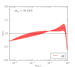
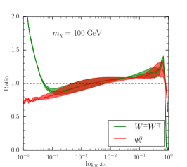
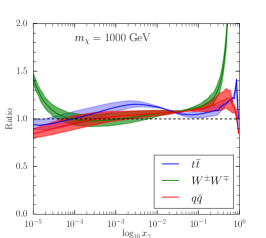
Figure 30: Photon spectra obtained using our tune normalized to the results of Cirelli:2010xx for $m_{\chi}=10$ GeV (left pane), $m_{\chi}=100$ GeV (center pane) and $m_{\chi}=1000$ GeV (right pane). The spectra are shown for DM annihilation into $q\bar{q}$ (red), $W^{\pm}W^{\mp}$ (green) and $t\bar{t}$ (blue). The dashed bands show the QCD uncertainties on the parameters of the Lund fragmentation function.

Appendix D Our results relative to the PPPC4DMID

The PPPC4DMID Cirelli:2010xx is widely used for DM studies. The authors of Cirelli:2010xx made a detailed MC study of particle spectra in DM annihilation including Electro-Weak (EW) corrections Ciafaloni:2010ti . The output of this study was a complete recipe, in the form of interpolating grids, for particle spectra ($\gamma,e^{+},\bar{p},\bar{\nu}\ldots$) in DM annihilation covering a wide range of DM masses (from $5$ GeV to $100$ TeV) and annihilation channels.

The spectra currently available in the PPPC4DMID were obtained using Pythia version 8.135, which was published in January 2010. Since then, a number of salient changes and updates have been made to the Pythia code. Firstly, the original default tune parameters (which were poorly documented but dated from around 2009) were replaced, in Pythia 8.2, by the Monash 2013 tune Skands:2014pea , which included a complete overhaul of the final-state fragmentation parameters. Secondly, additional capabilities are available in the newer version we use for this study, such as QED showering off heavy charged particles (e.g., $W$ bosons and top quarks) which can have important contributions when they are produced very far from their threshold as was discussed in section 2. A more complete list of changes (relative to when the original PPPC4DMID study was done) relevant to the modeling of photon spectra in final-state fragmentation processes is as follows:

• Pythia 8.135: version used for the cookbook.

• Pythia 8.170: particle masses, widths, and decay branching fractions updated using the PDG 2012 values.

• Pythia 8.175: new option included (off by default) to allow photon radiation in leptonic two-body decays of hadrons, via ParticleDecays:allowPhotonRadiation = on.

• Pythia 8.175: The lower shower cutoff TimeShower:pTminChgL for photon radiation off charged leptons was reduced from $0.0005$ to $10^{-6}$.

• Pythia 8.176: new option for weak showers introduced (off by default).

• Pythia 8.200: default tune parameters changed to those of the Monash 2013 tune. The default tune parameter values from 8.135 are still available as an option using Tune:ee = 3.

• Pythia 8.219: new flag TimeShower:QEDshowerByOther allows charged resonances like $W^{\pm}$ to radiate photons.

We therefore believe that it would be useful to provide our results as updates to the PPPC4DMID tables. These are available from the authors of this study, and will also be released publicly in a future update. (We also note that the EW corrections considered in the PPPC4DMID study factorize off the non-perturbative QCD modeling and they can be added to our predictions without any problem).

To illustrate the numerical size of the differences, we display in Fig. 30 the ratio of our predictions to the results of Cirelli:2010xx in the photon spectra for three DM masses; $m_{\chi}=10,100$ and $1000$ GeV. We have chosen three final states, i.e $q\bar{q},q=u,d,s$, $W^{\pm}W^{\mp}$ and $t\bar{t}$. We can see that the relative differences between our tuning and the predictions of the Cookbook can be quite important, particularly in the edges of the distributions (small $x_{\gamma}$ and large $x_{\gamma}$). As these differences cannot be accounted for by QCD uncertainties (shown as dashed bands in Fig. 30), we urge to use the updated predictions from this study.

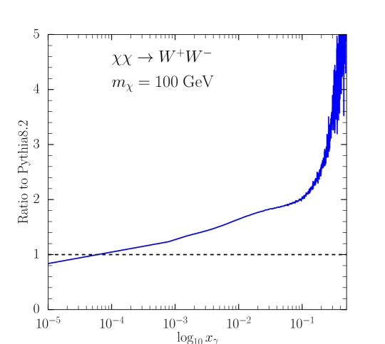
Figure 31: Photon spectra obtained using the fit functions given in Cembranos:2010dm normalized to the results of our tune for $\chi\chi\to W^{+}W^{-}$ and $m_{\chi}=100$ GeV.

Before closing this section, we would like to shortly discuss the comparison with the predictions of Pythia6-418 used in an analysis done by the authors of Cembranos:2010dm . In Cembranos:2010dm , a complete analysis of the photon spectra in WIMP DM annihilation has been performed and fitting functions have been provided for different DM masses, and annihilation channels. As an example, we compare our predictions with those obtained in Eqn. 8 of Cembranos:2010dm for $\chi\chi\to W^{+}W^{-}$ with $m_{\chi}=100$ GeV. We display the results of the comparisons in Fig. 31. We find that the agreement is relatively not so good as compared to the PPP 4 DMID (medium panel of Fig. 30) especially in the peak region. This suggests that the improvements in Pythia MC event generator are converging to solid picture thanks to the developments of the used models as well as the wealth of data that were used to tune the parameters.

References

- (1) G. Bertone, D. Hooper, and J. Silk, Particle dark matter: Evidence, candidates and constraints, Phys.Rept. 405 (2005) 279–390, [hep-ph/0404175].
- (2) Planck Collaboration, P. A. R. Ade et al., Planck 2015 results. XIII. Cosmological parameters, Astron. Astrophys. 594 (2016) A13, [arXiv:1502.01589].
- (3) Fermi/LAT Collaboration, Fermi-LAT Observations of High-Energy Gamma-Ray Emission Toward the Galactic Center, arXiv:1511.02938.
- (4) L. Goodenough and D. Hooper, Possible Evidence For Dark Matter Annihilation In The Inner Milky Way From The Fermi Gamma Ray Space Telescope, arXiv:0910.2998.
- (5) Fermi/LAT Collaboration, Indirect Search for Dark Matter from the center of the Milky Way with the Fermi-Large Area Telescope, arXiv:0912.3828.
- (6) D. Hooper and L. Goodenough, Dark Matter Annihilation in The Galactic Center As Seen by the Fermi Gamma Ray Space Telescope, Phys. Rev. B697 (2011) 412–428, [arXiv:1010.2752].
- (7) C. Gordon and O. Macias, Dark Matter and Pulsar Model Constraints from Galactic Center Fermi-LAT Gamma Ray Observations, Phys. Rev. D88 (2013) 083521, [arXiv:1306.5725].
- (8) D. Hooper and T. Linden, On The Origin Of The Gamma Rays From The Galactic Center, Phys. Rev. D84 (2011) 123005, [arXiv:1110.0006].
- (9) T. Daylan, D. P. Finkbeiner, D. Hooper, T. Linden, S. K. N. Portillo, et al., The Characterization of the Gamma-Ray Signal from the Central Milky Way: A Compelling Case for Annihilating Dark Matter, arXiv:1402.6703.
- (10) F. Calore, I. Cholis, and C. Weniger, Background model systematics for the Fermi GeV excess, JCAP 1503 (2015) 038, [arXiv:1409.0042].
- (11) K. N. Abazajian, N. Canac, S. Horiuchi, and M. Kaplinghat, Astrophysical and Dark Matter Interpretations of Extended Gamma-Ray Emission from the Galactic Center, Phys. Rev. D90 (2014), no. 2 023526, [arXiv:1402.4090].
- (12) B. Zhou, Y.-F. Liang, X. Huang, X. Li, Y.-Z. Fan, et al., GeV excess in the Milky Way: Depending on Diffuse Galactic gamma ray Emission template?, arXiv:1406.6948.
- (13) A. Achterberg, S. Amoroso, S. Caron, L. Hendriks, R. Ruiz de Austri, and C. Weniger, A description of the Galactic Center excess in the Minimal Supersymmetric Standard Model, JCAP 1508 (2015), no. 08 006, [arXiv:1502.05703].
- (14) G. Bertone, F. Calore, S. Caron, R. Ruiz de Austri, J. S. Kim, R. Trotta, and C. Weniger, Global analysis of the pMSSM in light of the Fermi GeV excess: prospects for the LHC Run-II and astroparticle experiments, ArXiv e-prints (July, 2015) [arXiv:1507.07008].
- (15) A. Butter, S. Murgia, T. Plehn, and T. M. P. Tait, Saving the MSSM from the Galactic Center Excess, Phys. Rev. D96 (2017), no. 3 035036, [arXiv:1612.07115].
- (16) A. Achterberg, M. van Beekveld, S. Caron, G. A. Gómez-Vargas, L. Hendriks, and R. Ruiz de Austri, Implications of the Fermi-LAT Pass 8 Galactic Center excess on supersymmetric dark matter, JCAP 1712 (2017), no. 12 040, [arXiv:1709.10429].
- (17) A. Metz and A. Vossen, Parton Fragmentation Functions, Prog. Part. Nucl. Phys. 91 (2016) 136–202, [arXiv:1607.02521].
- (18) X. Artru and G. Mennessier, String model and multiproduction, Nucl. Phys. B70 (1974) 93–115.
- (19) B. Andersson, G. Gustafson, G. Ingelman, and T. Sjostrand, Parton Fragmentation and String Dynamics, Phys. Rept. 97 (1983) 31–145.
- (20) B. R. Webber, A QCD Model for Jet Fragmentation Including Soft Gluon Interference, Nucl. Phys. B238 (1984) 492–528.
- (21) J.-C. Winter, F. Krauss, and G. Soff, A Modified cluster hadronization model, Eur. Phys. J. C36 (2004) 381–395, [hep-ph/0311085].
- (22) A. Buckley et al., General-purpose event generators for LHC physics, Phys. Rept. 504 (2011) 145–233, [arXiv:1101.2599].
- (23) J. A. R. Cembranos, A. de la Cruz-Dombriz, V. Gammaldi, R. A. Lineros, and A. L. Maroto, Reliability of Monte Carlo event generators for gamma ray dark matter searches, JHEP 09 (2013) 077, [arXiv:1305.2124].
- (24) A. Buckley, H. Hoeth, H. Lacker, H. Schulz, and J. E. von Seggern, Systematic event generator tuning for the LHC, Eur. Phys. J. C65 (2010) 331–357, [arXiv:0907.2973].
- (25) A. Buckley, J. Butterworth, L. Lonnblad, D. Grellscheid, H. Hoeth, J. Monk, H. Schulz, and F. Siegert, Rivet user manual, Comput. Phys. Commun. 184 (2013) 2803–2819, [arXiv:1003.0694].
- (26) P. Z. Skands, Tuning Monte Carlo Generators: The Perugia Tunes, Phys. Rev. D82 (2010) 074018, [arXiv:1005.3457].
- (27) S. Platzer and S. Gieseke, Dipole Showers and Automated NLO Matching in Herwig++, Eur. Phys. J. C72 (2012) 2187, [arXiv:1109.6256].
- (28) A. Karneyeu, L. Mijovic, S. Prestel, and P. Z. Skands, MCPLOTS: a particle physics resource based on volunteer computing, Eur. Phys. J. C74 (2014) 2714, [arXiv:1306.3436].
- (29) P. Skands, S. Carrazza, and J. Rojo, Tuning PYTHIA 8.1: the Monash 2013 Tune, Eur. Phys. J. C74 (2014), no. 8 3024, [arXiv:1404.5630].
- (30) N. Fischer, S. Gieseke, S. Plätzer, and P. Skands, Revisiting radiation patterns in collisions, Eur. Phys. J. C74 (2014), no. 4 2831, [arXiv:1402.3186].
- (31) N. Fischer, S. Prestel, M. Ritzmann, and P. Skands, Vincia for Hadron Colliders, Eur. Phys. J. C76 (2016), no. 11 589, [arXiv:1605.06142].
- (32) D. Reichelt, P. Richardson, and A. Siodmok, Improving the Simulation of Quark and Gluon Jets with Herwig 7, Eur. Phys. J. C77 (2017), no. 12 876, [arXiv:1708.01491].
- (33) J. Kile and J. von Wimmersperg-Toeller, Monte Carlo Tuning for Hadrons and Comparison with Unfolded LEP Data, arXiv:1706.02242.
- (34) T. Sjöstrand, S. Ask, J. R. Christiansen, R. Corke, N. Desai, P. Ilten, S. Mrenna, S. Prestel, C. O. Rasmussen, and P. Z. Skands, An Introduction to PYTHIA 8.2, Comput. Phys. Commun. 191 (2015) 159–177, [arXiv:1410.3012].
- (35) T. Sjostrand and P. Z. Skands, Transverse-momentum-ordered showers and interleaved multiple interactions, Eur. Phys. J. C39 (2005) 129–154, [hep-ph/0408302].
- (36) S. Catani, B. R. Webber, and G. Marchesini, QCD coherent branching and semiinclusive processes at large x, Nucl. Phys. B349 (1991) 635–654.
- (37) S. Mrenna and P. Skands, Automated Parton-Shower Variations in Pythia 8, Phys. Rev. D94 (2016), no. 7 074005, [arXiv:1605.08352].
- (38) Particle Data Group Collaboration, C. Patrignani et al., Review of Particle Physics, Chin. Phys. C40 (2016), no. 10 100001.
- (39) ALEPH Collaboration, R. Barate et al., Studies of quantum chromodynamics with the ALEPH detector, Phys. Rept. 294 (1998) 1–165.
- (40) DELPHI Collaboration, P. Abreu et al., Tuning and test of fragmentation models based on identified particles and precision event shape data, Z. Phys. C73 (1996) 11–60.
- (41) P. Skands, Introduction to QCD, in Proceedings, 2nd Asia-Europe-Pacific School of High-Energy Physics (AEPSHEP 2014): Puri, India, November 04–17, 2014, pp. 341–420, 2013. arXiv:1207.2389. [,63(2107)].
- (42) L3 Collaboration, B. Adeva et al., Measurement of the inclusive production of neutral pions and charged particles on the Z0 resonance, Phys. Lett. B259 (1991) 199–208.
- (43) DELPHI Collaboration, W. Adam et al., Measurement of inclusive pi0 production in hadronic Z0 decays, Z. Phys. C69 (1996) 561–574.
- (44) ALEPH Collaboration, R. Barate et al., Inclusive production of neutral pions in hadronic Z decays, Z. Phys. C74 (1997) 451–461.
- (45) OPAL Collaboration, K. Ackerstaff et al., Photon and light meson production in hadronic Z0 decays, Eur. Phys. J. C5 (1998) 411–437, [hep-ex/9805011].
- (46) ALEPH Collaboration, D. Buskulic et al., Measurement of the production rates of eta and eta-prime in hadronic Z decays, Phys. Lett. B292 (1992) 210–220.
- (47) L3 Collaboration, O. Adriani et al., Measurement of inclusive eta production in hadronic decays of the Z0, Phys. Lett. B286 (1992) 403–412.
- (48) ALEPH Collaboration, A. Heister et al., Inclusive production of the omega and eta mesons in Z decays, and the muonic branching ratio of the omega, Phys. Lett. B528 (2002) 19–33, [hep-ex/0201012].
- (49) SLD Collaboration, K. Abe et al., Production of pi+, K+, K0, K*0, phi, p and Lambda0 in hadronic Z0 decays, Phys. Rev. D59 (1999) 052001, [hep-ex/9805029].
- (50) J. Bellm et al., Herwig 7.0/Herwig++ 3.0 release note, Eur. Phys. J. C76 (2016), no. 4 196, [arXiv:1512.01178].
- (51) S. Gieseke, P. Stephens, and B. Webber, New formalism for QCD parton showers, JHEP 12 (2003) 045, [hep-ph/0310083].
- (52) S. Platzer and S. Gieseke, Coherent Parton Showers with Local Recoils, JHEP 01 (2011) 024, [arXiv:0909.5593].
- (53) T. Gleisberg, S. Hoeche, F. Krauss, M. Schonherr, S. Schumann, F. Siegert, and J. Winter, Event generation with SHERPA 1.1, JHEP 02 (2009) 007, [arXiv:0811.4622].
- (54) S. Schumann and F. Krauss, A Parton shower algorithm based on Catani-Seymour dipole factorisation, JHEP 03 (2008) 038, [arXiv:0709.1027].
- (55) T. Sjostrand, S. Mrenna, and P. Z. Skands, PYTHIA 6.4 Physics and Manual, JHEP 0605 (2006) 026, [hep-ph/0603175].
- (56) ALEPH Collaboration, A. Heister et al., Studies of QCD at e+ e- centre-of-mass energies between 91-GeV and 209-GeV, Eur. Phys. J. C35 (2004) 457–486.
- (57) L3 Collaboration, P. Achard et al., Studies of hadronic event structure in annihilation from 30-GeV to 209-GeV with the L3 detector, Phys. Rept. 399 (2004) 71–174, [hep-ex/0406049].
- (58) F. James and M. Roos, Minuit: A System for Function Minimization and Analysis of the Parameter Errors and Correlations, Comput. Phys. Commun. 10 (1975) 343–367.
- (59) ALEPH Collaboration, D. Decamp et al., Measurement of the charged particle multiplicity distribution in hadronic Z decays, Phys. Lett. B273 (1991) 181–192.
- (60) ALEPH Collaboration, D. Buskulic et al., First measurement of the quark to photon fragmentation function, Z. Phys. C69 (1996) 365–378.
- (61) DELPHI Collaboration, P. Abreu et al., Charged particle multiplicity distributions in Z0 hadronic decays, Z. Phys. C50 (1991) 185–194.
- (62) L3 Collaboration, M. Acciarri et al., Measurement of inclusive production of neutral hadrons from Z decays, Phys. Lett. B328 (1994) 223–233.
- (63) OPAL Collaboration, R. Akers et al., Measurement of the production rates of charged hadrons in e+ e- annihilation at the Z0, Z. Phys. C63 (1994) 181–196.
- (64) OPAL Collaboration, K. Ackerstaff et al., Measurements of flavor dependent fragmentation functions in Z0 –> q anti-q events, Eur. Phys. J. C7 (1999) 369–381, [hep-ex/9807004].
- (65) OPAL Collaboration, G. Abbiendi et al., Measurement of event shape distributions and moments in e+ e- —> hadrons at 91-GeV - 209-GeV and a determination of alpha(s), Eur. Phys. J. C40 (2005) 287–316, [hep-ex/0503051].
- (66) SLD Collaboration, K. Abe et al., Measurement of the charged multiplicities in b, c and light quark events from Z0 decays, Phys. Lett. B386 (1996) 475–485, [hep-ex/9608008].
- (67) SLD Collaboration, K. Abe et al., Production of pi+, pi-, K+, K-, p and anti-p in light (uds), c and b jets from Z0 decays, Phys. Rev. D69 (2004) 072003, [hep-ex/0310017].
- (68) CTA Collaboration, R. A. Ong, Cherenkov Telescope Array: The Next Generation Gamma-ray Observatory, PoS ICRC2017 (2018) 1071, [arXiv:1709.05434].
- (69) M. Cirelli, G. Corcella, A. Hektor, G. Hutsi, M. Kadastik, et al., PPPC 4 DM ID: A Poor Particle Physicist Cookbook for Dark Matter Indirect Detection, JCAP 1103 (2011) 051, [arXiv:1012.4515].
- (70) M. G. Bowler, e+ e- Production of Heavy Quarks in the String Model, Z. Phys. C11 (1981) 169.
- (71) S. Argyropoulos and T. Sjostrand, Effects of color reconnection on final states at the LHC, JHEP 11 (2014) 043, [arXiv:1407.6653].
- (72) CMS Collaboration, A. M. Sirunyan et al., Measurement of the top quark mass with lepton+jets final states using collisions at , Eur. Phys. J. C78 (2018), no. 11 891, [arXiv:1805.01428].
- (73) ALEPH Collaboration, D. Buskulic et al., Inclusive pi+-, K+- and (p, anti-p) differential cross-sections at the Z resonance, Z. Phys. C66 (1995) 355–366.
- (74) Particle Data Group Collaboration, C. Amsler et al., Review of Particle Physics, Phys. Lett. B667 (2008) 1–1340.
- (75) J. Alwall et al., A Standard format for Les Houches event files, Comput. Phys. Commun. 176 (2007) 300–304, [hep-ph/0609017].
- (76) P. Ciafaloni, D. Comelli, A. Riotto, F. Sala, A. Strumia, and A. Urbano, Weak Corrections are Relevant for Dark Matter Indirect Detection, JCAP 1103 (2011) 019, [arXiv:1009.0224].
- (77) J. A. R. Cembranos, A. de la Cruz-Dombriz, A. Dobado, R. A. Lineros, and A. L. Maroto, Photon spectra from WIMP annihilation, Phys. Rev. D83 (2011) 083507, [arXiv:1009.4936].