The initial-boundary value problems for the coupled derivative nonlinear Schrödinger equations on the half-line

Abstract: The unified transform method is used to analyze the initial-boundary value problem for the coupled derivative nonlinear Schrödinger(CDNLS) equations on the half-line. In this paper, we assume that the solution $u(x,t)$ and $v(x,t)$ of CDNLS equations are exists, and we show that it can be expressed in terms of the unique solution of a matrix Riemann-Hilbert problem formulated in the plane of the complex spectral parameter $\lambda$.

Keywords Riemann-Hilbert problem; CDNLS equations; Initial-boundary value problem; unified transform method
MSC(2010) 35G31, 35Q15, 35Q51

1 Introduction

Since the 1960s, the inverse scattering method with the initial value problem give mathematical physicists great power to find exact solution of the nonlinear partial differential equations. This includes continuity and discrete partial differential equations (usually we call soliton equations because they have soliton solutions). Thanks to four mathematicians Gardner, Greene, Kruskal and Miura. They initially studied KdV equation exact solution (1967,1974) with the initial value problem. Because this method can have the power of infinite life for the whole family of equations, and has been applied to many scientific and technological fields including geophysical prospecting, super symmetric quantum mechanics and so on. But for the initial boundary value(IBV) problem of the soliton equation, how to find their exact solution? This is a very big challenge problem. Fortunately, in general as long as the equation is integrable, these problems can be solved. Here integrable are equations which have Lax pairs.

In 1997, Fokas used inverse scattering transform(IST) thought to construct a new unified method, we call this method as Fokas method. He analyzed the IBV problems for linear and nonlinear integrable PDEs[1, 2, 3]. In the past 20 years, the unified method has been used to analyse boundary value problems for several of the most important integrable equations with $2\times 2$ matrix Lax pairs, such as the Korteweg-deVries(KdV) equation, the nonlinear Schrödinger(NLS) equation, the sine-Gordon(sG) equation, the derivative NLS(DNLS) equation and the complex Sharma-Tasso-Olver(CSTO) equation [4-8], etc. Just like the IST on the line, the unified method provides an expression for the solution of an IBV problem in terms of the solution of a Riemann-Hilbert problem. In particular, by analyzing the asymptotic behaviour of the solution based on this Riemann-Hilbert problem and by employing the nonlinear version of the steepest descent method introduced by Deift and Zhou [9] in 1993. In this way, the long time asymptotics for the solutions of decay initial value problem of NLS equation and the MKdV equation were analyzed respectively by Deift and Zhou [9, 10]. The DNLS and other integrable equations have been rigorously established [11-14]. For the asymptotics of the solution of IBV problem and step-like initial value problem for the DNLS also have been considered [15, 16].

In 2012, Lenells[17] applied the unified transform method to analyse IBV problems for integrable evolution equations whose Lax pairs involving $3\times 3$ matrices, and following this method, the IBV problems for the Degasperis-Procesi equation to be studied in[18]. After that, most important integrable equations IBV problems for integrable evolution equations with higher order Lax pairs to be studied [19-28]. we also have a good time to study partial differential equations with IBV problem on the basis of these giants. In this paper, we would like to analyse the IBV problem of the following coupled DNLS equation[29, 30, 31]:

$$\left\{\begin{array}[]{l}iu_{t}+u_{xx}+i\gamma[(|u|^{2}+|v|^{2})u]_{x}=0,\\ iv_{t}+v_{xx}+i\gamma[(|u|^{2}+|v|^{2})v]_{x}=0.\end{array}\right.$$ (1.3)

on the half-line domain $\Omega=\{0<x<\infty,0<t<T\}$. Throughout this paper, we consider the following IBV problems for the CDNLS equations

$$\begin{array}[]{l}$Initial values$:u_{0}(x)=u(x,t=0),\;v_{0}(x)=v(x,t=0);\\ $Dirichlet boundary values$:g_{0}(t)=u(x=0,t),\;h_{0}(t)=v(x=0,t);\\ $Neumann boundary values$:g_{1}(t)=u_{x}(x=0,t),\;h_{1}(t)=v_{x}(x=0,t).\end{array}$$ (1.7)

where $u_{0}(x)$ and $v_{0}(x)$ lie in the Schwartz space.

This paper is organized as follows. In the next section, we define two sets of eigenfunctions $\mu_{j}(j=1,2,3)$ and $M_{n}(n=1,2,3,4)$ of Lax pair for spectral analysis. In addition, we also get some spectral functions satisfying the so-called global relation in this part. In the last section, we show that $u(x,t),v(x,t)$ can be expressed in terms of the unique solution of a matrix Riemann-Hilbert problem.

2 The spectral analysis

Consider the Lax pair of equations (1.1) as follows[32]

$$\left\{\begin{array}[]{l}\psi_{x}=U\psi=(-\frac{1}{\gamma}i\lambda^{2}\Lambda+\lambda U_{1})\psi,\\ \psi_{t}=V\psi=(\frac{2}{\gamma^{2}}i\lambda^{4}\Lambda-\frac{2}{\gamma}\lambda^{3}U_{1}+i\lambda^{2}U_{2}-\gamma\lambda U_{3})\psi,\end{array}\right.$$ (2.3)

where

$$\begin{array}[]{l}\Lambda=\left(\begin{array}[]{ccc}-1&0&0\\ 0&1&0\\ 0&0&1\end{array}\right),U_{1}=\left(\begin{array}[]{ccc}0&u&v\\ \bar{u}&0&0\\ \bar{v}&0&0\end{array}\right),U_{2}=\left(\begin{array}[]{ccc}-(|u|^{2}+|v|^{2})&0&0\\ 0&|u|^{2}&\bar{u}v\\ 0&u\bar{v}&|v|^{2}\end{array}\right),\\ U_{3}=\left(\begin{array}[]{ccc}0&u(|u|^{2}+|v|^{2})-iu_{x}&v(|u|^{2}+|v|^{2})-iv_{x}\\ \bar{u}(|u|^{2}+|v|^{2})+i\bar{u}_{x}&0&0\\ \bar{v}(|u|^{2}+|v|^{2})+i\bar{v}_{x}&0&0\end{array}\right).\end{array}$$ (2.18)

where the overbar represents the complex conjugation (similarly hereinafter), $\lambda$ is a spectral parameter, and $\psi(x,t,\lambda)$ is a vector or a matrix function. Throughout this paper, we set $\gamma=1$ for the convenient of the analysis.

2.1 The closed one-form

We are not difficult to find that Eq.(2.1) is equivalent to

$$\left\{\begin{array}[]{l}\psi_{x}+i\lambda^{2}\Lambda\psi=V_{1}\psi,\\ \psi_{t}-2i\lambda^{4}\Lambda\psi=V_{2}\psi,\end{array}\right.$$ (2.21)

where

$$V_{1}=\lambda U_{1},\quad V_{2}=-2\lambda^{3}U_{1}+i\lambda^{2}U_{2}-\lambda U_{3}.$$ (2.22)

We assume that $u(x,t),v(x,t)$ is a sufficiently smooth function in the half-line region $\Omega=\{0<x<\infty,0<t<T\}$, and decays sufficiently when $x\rightarrow\infty.$ Introducing a new function $\mu(x,t,\lambda)$ by

$$\psi=\mu e^{-i\lambda^{2}\Lambda x+2i\lambda^{4}\Lambda t},$$ (2.23)

then the Lax pair Eq.(2.3) becomes

$$\left\{\begin{array}[]{l}\mu_{x}+i\lambda^{2}[\Lambda,\mu]=V_{1}\mu,\\ \mu_{t}-2i\lambda^{4}[\Lambda,\mu]=V_{2}\mu,\end{array}\right.$$ (2.26)

and Eq.(2.6) can be written to the differential form

$$d(e^{i\lambda^{2}\hat{\Lambda}x-2i\lambda^{4}\hat{\Lambda}t}\mu)=W(x,t,\lambda),$$ (2.27)

where $W(x,t,\lambda)$ defined by

$$W(x,t,\lambda)=e^{(i\lambda^{2}x-2i\lambda^{4}t)\hat{\Lambda}}(V_{1}dx+V_{2}dt)\mu,$$ (2.28)

and $\hat{\Lambda}$ represents a matrix operator acting on $3\times 3$ matrix B by $\hat{\Lambda}B=[\Lambda,B]$.

2.2 The eigenfunction

Based on the Volterra integral equation, there are three eigenfunctions $\mu_{j}(x,t,\lambda)(j=1,2,3)$ of Eq.(2.6) defined as

$$\mu_{j}(x,t,\lambda)=\mathbb{I}+\int_{\gamma_{j}}e^{(-i\lambda^{2}x+2i\lambda^{4}t)\hat{\Lambda}}W_{j}(\xi,\tau,\lambda),\quad j=1,2,3,$$ (2.29)

where $W_{j}$ is determined Eq.(2.8), it is only used $\mu_{j}$ in place of $\mu$, and the contours $\gamma_{j}(j=1,2,3)$ are shown in figure 1.

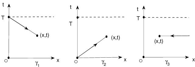
Figure 1: The three contours $\gamma_{1},\gamma_{2},\gamma_{3}$ in the $(x,t)$-domaint

The first, second, and third columns of the matrix equation (2.9) contain the following exponential term

$$\begin{array}[]{l}\mu_{j}^{(1)}:\quad e^{-2i\lambda^{2}(x-\xi)+4i\lambda^{4}(t-\tau)},e^{-2i\lambda^{2}(x-\xi)+4i\lambda^{4}(t-\tau)};\\ \mu_{j}^{(2)}:\quad e^{2i\lambda^{2}(x-\xi)-4i\lambda^{4}(t-\tau)};\\ \mu_{j}^{(3)}:\quad e^{2i\lambda^{2}(x-\xi)-4i\lambda^{4}(t-\tau)}.\end{array}$$ (2.33)

At the same time, the following inequalities hold true on the contours

$$\begin{array}[]{l}\gamma_{1}:\quad x-\xi\geq 0,\quad t-\tau\leq 0;\\ \gamma_{2}:\quad x-\xi\geq 0,\quad t-\tau\geq 0;\\ \gamma_{3}:\quad x-\xi\leq 0.\\ \end{array}$$ (2.37)

Thus, we can show that the eigenfunctions $\mu_{j}(x,t,\lambda)(j=1,2,3)$ are bounded and analytic for $\lambda\in\mathbb{C}$ such that $\lambda$ belongs to

$$\begin{array}[]{l}\mu_{1}$ is bounded and analytic for $\lambda\in(D_{4},D_{1},D_{1}),\\ \mu_{2}$ is bounded and analytic for $\lambda\in(D_{3},D_{2},D_{2}),\\ \mu_{3}$ is bounded and analytic for $\lambda\in(D_{1}\cup D_{2},D_{3}\cup D_{4},D_{3}\cup D_{4}),\\ \end{array}$$ (2.41)

where $D_{n}(n=1,2,3,4)$ denote four open, pairwisely disjoint subsets of the Riemann $\lambda$-plane shown in figure 2.

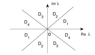
Figure 2: The sets $D_{j},j=1,2,3,4$, which decompose the complex $\lambda-$plane

And these sets $D_{n}(n=1,2,3,4)$ have the following properties:

$$\begin{array}[]{l}D_{1}=\{\lambda\in\mathbb{C}|Rel_{1}<Rel_{2}=Rel_{3},\quad Rez_{1}>Rez_{2}=Rez_{3}\},\\ D_{2}=\{\lambda\in\mathbb{C}|Rel_{1}<Rel_{2}=Rel_{3},\quad Rez_{1}<Rez_{2}=Rez_{3}\},\\ D_{3}=\{\lambda\in\mathbb{C}|Rel_{1}>Rel_{2}=Rel_{3},\quad Rez_{1}>Rez_{2}=Rez_{3}\},\\ D_{4}=\{\lambda\in\mathbb{C}|Rel_{1}>Rel_{2}=Rel_{3},\quad Rez_{1}<Rez_{2}=Rez_{3}\},\end{array}$$ (2.46)

where $l_{i}(\lambda)$ and $z_{i}(\lambda)$ are the diagonal elements of the matrix $-i\lambda^{2}\Lambda$ and $2i\lambda^{4}\Lambda$.

Specially, we can show that $\mu_{1}(0,t,\lambda)$ is bounded and analytic for $\lambda\in(D_{2}\cup D_{4},D_{1}\cup D_{3},D_{1}\cup D_{3})$, and $\mu_{2}(0,t,\lambda)$ is bounded and analytic for $\lambda\in(D_{1}\cup D_{3},D_{2}\cup D_{4},D_{2}\cup D_{4})$.

For each $n=1,2,3,4$, based on the following integral equation, the solution $M_{n}(x,t,\lambda)$ of Eq.(2.6) can be defined as

$$(M_{n}(x,t,\lambda))_{ij}=\delta_{ij}+\int_{\gamma_{ij}^{n}}(e^{(-i\lambda^{2}x+2i\lambda^{4}t)\hat{\sigma}}W_{n}(\xi,\tau,\lambda))_{ij},\quad i,j=1,2,3,$$ (2.47)

where $W_{n}(x,t,\lambda)$ is determined by Eq.(2.8), it is only used $M_{n}$ in place of $\mu$, and the contours $\gamma_{ij}^{n}(n=1,2,3,4;i,j=1,2,3)$ are defined as

$$\gamma_{ij}^{n}=\left\{\begin{array}[]{l}\gamma_{1}\quad if\quad Rel_{i}(\lambda)<Rel_{j}(\lambda)\quad and\quad Rez_{i}(\lambda)\geq Rez_{j}(\lambda),\\ \gamma_{2}\quad if\quad Rel_{i}(\lambda)<Rel_{j}(\lambda)\quad and\quad Rez_{i}(\lambda)<Rez_{j}(\lambda),for\lambda\in D_{n}\\ \gamma_{3}\quad if\quad Rel_{i}(\lambda)\geq Rel_{j}(\lambda).\end{array}\right.$$ (2.48)

Based on the definition of $\gamma^{n}$, we have

$$\begin{array}[]{l}\gamma^{1}=\left(\begin{array}[]{ccc}\gamma_{3}&\gamma_{1}&\gamma_{1}\\ \gamma_{3}&\gamma_{3}&\gamma_{3}\\ \gamma_{3}&\gamma_{3}&\gamma_{3}\end{array}\right),\quad\gamma^{2}=\left(\begin{array}[]{ccc}\gamma_{3}&\gamma_{2}&\gamma_{2}\\ \gamma_{3}&\gamma_{3}&\gamma_{3}\\ \gamma_{3}&\gamma_{3}&\gamma_{3}\end{array}\right),\\ \gamma^{3}=\left(\begin{array}[]{ccc}\gamma_{3}&\gamma_{3}&\gamma_{3}\\ \gamma_{2}&\gamma_{3}&\gamma_{3}\\ \gamma_{2}&\gamma_{3}&\gamma_{3}\end{array}\right),\quad\gamma^{4}=\left(\begin{array}[]{ccc}\gamma_{3}&\gamma_{3}&\gamma_{3}\\ \gamma_{1}&\gamma_{3}&\gamma_{3}\\ \gamma_{1}&\gamma_{3}&\gamma_{3}\end{array}\right).\end{array}$$ (2.63)

Next, the following proposition guarantees that the previous definition of $M_{n}$ has properties, namely, $M_{n}$ can be represented as a Rimann-Hilbert problem.

Proposition 2.1

For each $n=1,2,3,4$ and $\lambda\in D_{n}$, the function $M_{n}(x,t,\lambda)$ is defined well by Eq.(2.14). And for any identified point $(x,t)$, $M_{n}$ is bounded and analytical as a function of $\lambda\in D_{n}$ away from a possible discrete set of singularities $\{\lambda_{j}\}$ at which the Fredholm determinant vanishes. Moreover, $M_{n}$ admits a bounded and continuous extension to $\bar{D}_{n}$ and

$$M_{n}(x,t,\lambda)=\mathbb{I}+\mathcal{O}(\frac{1}{\lambda}).$$ (2.64)

Proof: The associated bounded and analytical properties have been established in Appendix B in [17]. Substituting the following expansion

$$M=M_{0}+\frac{M^{(1)}}{\lambda}+\frac{M^{(2)}}{\lambda^{2}}+\cdots\quad\quad\lambda\rightarrow\infty,$$

into the Lax pair Eq.(2.6) and comparing the coefficients of the same order of $\lambda$, we can obtain Eq.(2.17).

2.3 The jump matrix

Define the matrix-value functions as follows

$$S_{n}(\lambda)=M_{n}(0,0,\lambda),\quad\lambda\in D_{n},n=1,2,3,4.$$ (2.65)

Let $M$ be a sectionally analytical continuous function in Riemann $\lambda$-sphere which equals $M_{n}$ for $\lambda\in D_{n}$. Then $M$ satisfies the following jump conditions:

$$M_{n}(\lambda)=M_{m}J_{m,n},\quad\lambda\in\bar{D}_{n}\cap\bar{D}_{m},\quad n,m=1,2,3,4;n\neq m,$$ (2.66)

where

$$J_{m,n}=e^{(-i\lambda^{2}x+2i\lambda^{4}t)\hat{\Lambda}}(S_{m}^{-1}S_{n}).$$ (2.67)

2.4 The adjugated eigenfunction

To obtain the analyticity and boundedness properties of the minors of the matrices $\mu_{j}(x,t,\lambda)(j=1,2,3)$. We need consider the cofactor matrix $B^{A}$ of a $3\times 3$ matrix $B$ is defined by

$$B^{A}=\left(\begin{array}[]{ccc}m_{11}(B)&-m_{12}(B)&m_{13}(B)\\ -m_{21}(B)&m_{22}(B)&-m_{23}(B)\\ m_{31}(B)&-m_{32}(B)&m_{33}(B)\end{array}\right),$$

where $m_{ij}(B)$ denote the $(ij)$th minor of $B$.

From Eq.(2.6) we find that the adjugated eigenfunction $\mu^{A}$ have the following Lax pair equations:

$$\left\{\begin{array}[]{l}\mu_{x}^{A}-i\lambda^{2}[\Lambda,\mu^{A}]=-V_{1}^{T}\mu^{A},\\ \mu_{t}^{A}+2i\lambda^{4}[\Lambda,\mu^{A}]=-V_{2}^{T}\mu^{A},\\ \end{array}\right.$$ (2.70)

where the superscript $T$ denotes a matrix transpose. Then the eigenfunctions $\mu_{j}(j=1,2,3)$ satisfy the following integral equations

$$\mu_{j}^{A}(x,t,\lambda)=\mathbb{I}-\int_{\gamma_{j}}e^{(i\lambda^{2}(x-\xi)-2i\lambda^{4}(t-\tau))\hat{\Lambda}}(V_{1}^{T}dx+V_{2}^{T}dt),\quad j=1,2,3.$$ (2.71)

Thus, we can obtain the adjugated eigenfunction satisfies the following analyticity and boundedness properties:

$$\begin{array}[]{l}\mu_{1}^{A}$ is bounded and analytic for $\lambda\in(D_{1},D_{4},D_{4}),\\ \mu_{2}^{A}$ is bounded and analytic for $\lambda\in(D_{2},D_{3},D_{3}),\\ \mu_{3}^{A}$ is bounded and analytic for $\lambda\in(D_{3}\cup D_{4},D_{1}\cup D_{2},D_{1}\cup D_{2}).\end{array}$$ (2.75)

Specially, we can show that $\mu_{1}^{A}(0,t,\lambda)$ is bounded and analytic for $\lambda\in(D_{1}\cup D_{3},D_{2}\cup D_{4},D_{2}\cup D_{4})$, and $\mu_{2}^{A}(0,t,\lambda)$ is bounded and analytic for $\lambda\in(D_{2}\cup D_{4},D_{1}\cup D_{3},D_{1}\cup D_{3})$.

2.5 Symmetry

We can show that the eigenfunctions $\mu_{j}(x,t,\lambda)$ have an important symmetry by the following Lemma.

Lemma 2.2

The eigenfunction $\psi(x,t,\lambda)$ of the Lax pair Eq.(2.1) have the following symmetry

$$\psi^{-1}(x,t,\lambda)=A\overline{\psi(x,t,\bar{\lambda})}^{T}A,$$

with

$$A=\left(\begin{array}[]{ccc}1&0&0\\ 0&-\varepsilon&0\\ 0&0&-\varepsilon\end{array}\right),\quad and\quad\varepsilon^{2}=1.$$

where the superscript $T$ denotes a matrix transpose.

Proof: Analogous to the proof provided in [17]. We omit the proof.

Remark 2.3

From Lemma 2.2, we can show that the eigenfunctions $\mu_{j}(x,t,\lambda)$ of Lax pair Eq.(2.6) have the same symmetry.

2.6 The jump matrix computations

We also define the $3\times 3$ matrix value spectral function $s(\lambda)$ and $S(\lambda)$ as follows

$$\left\{\begin{array}[]{l}\mu_{3}(x,t,\lambda)=\mu_{2}(x,t,\lambda)e^{(-i\lambda^{2}x+2i\lambda^{4}t)\hat{\Lambda}}s(\lambda),\\ \mu_{1}(x,t,\lambda)=\mu_{2}(x,t,\lambda)e^{(-i\lambda^{2}x+2i\lambda^{4}t)\hat{\Lambda}}S(\lambda),\end{array}\right.$$ (2.78)

by $\mu_{2}(0,0,\lambda)=\mathbb{I}$, and from Eq.(2.24) we can obtain

$$s(\lambda)=\mu_{3}(0,0,\lambda),\quad\quad S(\lambda)=\mu_{1}(0,0,\lambda).$$ (2.79)

From the properties of $\mu_{j}$ and $\mu_{j}^{A}(j=1,2,3)$, we can drive that $s(\lambda),S(\lambda),s^{A}(\lambda)$ and $S^{A}(\lambda)$ have the following bounded and analytic properties

$$\begin{array}[]{l}s(\lambda)$ is bounded for $\lambda\in(D_{1}\cup D_{2},D_{3}\cup D_{4},D_{3}\cup D_{4}),\\ S(\lambda)$ is bounded for $\lambda\in(D_{2}\cup D_{4},D_{1}\cup D_{3},D_{1}\cup D_{3}),\\ s^{A}(\lambda)$ is bounded for $\lambda\in(D_{3}\cup D_{4},D_{1}\cup D_{2},D_{1}\cup D_{2}),\\ S^{A}(\lambda)$ is bounded for $\lambda\in(D_{1}\cup D_{3},D_{2}\cup D_{4},D_{2}\cup D_{4}).\end{array}$$ (2.84)

Moreover

$$M_{n}(x,t,\lambda)=\mu_{2}(x,t,\lambda)e^{(-i\lambda^{2}x+2i\lambda^{4}t)\hat{\Lambda}}S_{n}(\lambda),\quad\lambda\in D_{n}.$$ (2.85)

Proposition 2.4

The $S_{n}$ can be expressed with $s(\lambda)$ and $S(\lambda)$ elements as follows

$$\begin{array}[]{l}S_{1}=\left(\begin{array}[]{ccc}s_{11}&\frac{m_{33}(s)M_{21}(S)-m_{23}(s)M_{31}(S)}{(s^{T}S^{A})_{11}}&\frac{m_{32}(s)M_{21}(S)-m_{22}(s)M_{31}(S)}{(s^{T}S^{A})_{11}}\\ s_{21}&\frac{m_{33}(s)M_{11}(S)-m_{13}(s)M_{31}(S)}{(s^{T}S^{A})_{11}}&\frac{m_{32}(s)M_{11}(S)-m_{12}(s)M_{31}(S)}{(s^{T}S^{A})_{11}}\\ s_{31}&\frac{m_{23}(s)M_{11}(S)-m_{13}(s)M_{21}(S)}{(s^{T}S^{A})_{11}}&\frac{m_{22}(s)M_{11}(S)-m_{12}(s)M_{21}(S)}{(s^{T}S^{A})_{11}}\end{array}\right),\\ S_{2}=\left(\begin{array}[]{ccc}s_{11}&0&0\\ s_{21}&\frac{m_{33}(s)}{s_{11}}&\frac{m_{32}(s)}{s_{11}}\\ s_{31}&\frac{m_{23}(s)}{s_{11}}&\frac{m_{22}(s)}{s_{11}}\end{array}\right),\quad S_{3}=\left(\begin{array}[]{ccc}\frac{1}{m_{11}(s)}&s_{12}&s_{13}\\ 0&s_{22}&s_{23}\\ 0&s_{32}&s_{33}\end{array}\right),\\ S_{4}=\left(\begin{array}[]{ccc}\frac{S_{11}}{(S^{T}s^{A})_{11}}&s_{12}&s_{13}\\ \frac{S_{21}}{(S^{T}s^{A})_{11}}&s_{22}&s_{23}\\ \frac{S_{31}}{(S^{T}s^{A})_{11}}&s_{32}&s_{33}\end{array}\right).\end{array}$$ (2.101)

where $(S^{T}s^{A})_{11}$ and $(s^{T}S^{A})_{11}$ are defined as follows

$$\begin{array}[]{l}(S^{T}s^{A})_{11}=S_{11}m_{11}(s)-S_{21}m_{21}(s)+S_{31}m_{31}(s),\\ (s^{T}S^{A})_{11}=s_{11}m_{11}(S)-s_{21}m_{21}(S)+s_{31}m_{31}(S).\end{array}$$ (2.104)

Proof: We set that $\gamma_{3}^{X_{0}}$ is a contour when $(X_{0},0)\rightarrow(x,t)$ in the $(x,t)$-plane, here $X_{0}$ is a constant and $X_{0}>0$, for $j=3$, we introduce $\mu_{3}(x,t,\lambda;X_{0})$ as the solution of Eq.(2.9) with the contour $\gamma_{3}$ replaced by $\gamma_{3}^{X_{0}}$. Similarly, we define $M_{n}(x,t,\lambda;X_{0})$ as the solution of Eq.(2.14) with $\gamma_{3}$ replaced by $\gamma_{3}^{X_{0}}$. then, by simple calculation, we can use $S(\lambda)$ and $s(\lambda;X_{0})=\mu_{3}(0,0,\lambda;X_{0})$ to derive the expression of $S_{n}(\lambda,X_{0})=M_{n}(0,0,\lambda;X_{0})$ and the Eq.(2.28) will be obtained by taking the limit $X_{0}\rightarrow\infty$.

Firstly, we have the following relations:

$$M_{n}(x,t,\lambda;X_{0})=\mu_{1}(x,t,\lambda)e^{(-i\lambda^{2}x+2i\lambda^{4}t)\hat{\Lambda}}R_{n}(\lambda;X_{0}),$$ (2.105)

$$M_{n}(x,t,\lambda;X_{0})=\mu_{2}(x,t,\lambda)e^{(-i\lambda^{2}x+2i\lambda^{4}t)\hat{\Lambda}}S_{n}(\lambda;X_{0}),$$ (2.106)

$$M_{n}(x,t,\lambda;X_{0})=\mu_{3}(x,t,\lambda)e^{(-i\lambda^{2}x+2i\lambda^{4}t)\hat{\Lambda}}T_{n}(\lambda;X_{0}).$$ (2.107)

Secondly, we can get the definition of $R_{n}(\lambda;X_{0})$ and $T_{n}(\lambda;X_{0})$ as follows

$$R_{n}(\lambda;X_{0})=e^{-2i\lambda^{4}T\hat{\Lambda}}M_{n}(0,T,\lambda;X_{0}),$$ (2.108)

$$T_{n}(\lambda;X_{0})=e^{i\lambda^{2}X_{0}\hat{\Lambda}}M_{n}(X_{0},0,\lambda;X_{0}),$$ (2.109)

then equations(2.29),(2.30) and (2.31) mean that

$$s(\lambda;X_{0})=S_{n}(\lambda;X_{0})T_{n}^{-1}(\lambda;X_{0}),\;S(\lambda;X_{0})=S_{n}(\lambda;X_{0})R_{n}^{-1}(\lambda;X_{0}).$$ (2.110)

These equations constitute the matrix decomposition problem of $\{s,S\}$ by use $\{R_{n},S_{n},T_{n}\}$. In fact, by the definition of the integral equation (2.14) and $\{R_{n},S_{n},T_{n}\}$, we obtain

$$\left\{\begin{array}[]{l}(R_{n}(\lambda;X_{0}))_{ij}=0\quad if\quad\gamma_{ij}^{n}=\gamma_{1},\\ (S_{n}(\lambda;X_{0}))_{ij}=0\quad if\quad\gamma_{ij}^{n}=\gamma_{2},\\ (T_{n}(\lambda;X_{0}))_{ij}=\delta_{ij}\quad if\quad\gamma_{ij}^{n}=\gamma_{3}.\end{array}\right.$$ (2.111)

Thus equations (2.35) is the 18 scalar equations with 18 unknowns. The exact solution of these system can be obtained by solving the algebraic system, in this way, we can get a similar $\{S_{n}(\lambda),s(\lambda)\}$ as in Eq.(2.28) which just that $\{S_{n}(\lambda),s(\lambda)\}$ replaces by $\{S_{n}(\lambda;X_{0}),s(\lambda;X_{0})\}$ in Eq.(2.28).

Finally, taking $X_{0}\rightarrow\infty$ in this equation, we obtain the Eq.(2.28).

2.7 The residue conditions

Because $\mu_{2}$ is an entire function, and from Eq.(2.27) we know that $M$ only produces singularities in $S_{n}$ where there are singular points, from the exact expression Eq.(2.28), we know that $M$ may be singular as follows

(1) $[M_{1}]_{2}$ and $[M_{1}]_{3}$ could have poles in $D_{1}$ at the zeros of $(s^{T}S^{A})_{11}(\lambda)$,

(2) $[M_{2}]_{2}$ and $[M_{2}]_{3}$ could have poles in $D_{2}$ at the zeros of $s_{11}(\lambda)$,

(3) $[M_{3}]_{1}$ could have poles in $D_{3}$ at the zeros of $m_{11}(s)(\lambda)$,

(4) $[M_{4}]_{1}$ could have poles in $D_{4}$ at the zeros of $(S^{T}s^{A})_{11}(\lambda)$.

We use $\lambda_{j}(j=1,2\cdots N)$ denote the possible zero point above, and assume that these zeros satisfy the following assumptions

Assumption 2.5

We assume that

(1)$(s^{T}S^{A})_{11}(\lambda)$ has $n_{0}$ possible simple zeros in $D_{1}$ denoted by $\lambda_{j},j=1,2\cdots n_{0}$,

(2)$s_{11}(\lambda)$ has $n_{1}-n_{0}$ possible simple zeros in $D_{2}$ denoted by $\lambda_{j},j=n_{0}+1,n_{0}+2\cdots n_{1}$,

(3)$m_{11}(s)(\lambda)$ has $n_{2}-n_{1}$ possible simple zeros in $D_{3}$ denoted by $\lambda_{j},j=n_{1}+1,n_{1}+2\cdots n_{2}$,

(4)$(S^{T}s^{A})_{11}(\lambda)$ has $N-n_{2}$ possible simple zeros in $D_{4}$ denoted by $\lambda_{j},j=n_{2}+2,n_{2}+2\cdots N$,

And these zeros are each different, moreover assuming that there is no zero on the boundary of $D_{n}(n=1,2,3,4)$.

Proposition 2.6

Let $M_{n}(n=1,2,3,4)$ be the eigenfunctions defined by (2.14) and assume that the set $\lambda_{j}(j=1,2\cdots N)$ of singularities are as the above assumption. Then the following residue conditions hold true:

$$\begin{array}[]{l}Res_{\lambda=\lambda_{j}}[M]_{2}=\frac{m_{33}(s)(\lambda_{j})M_{11}(S)(\lambda_{j})-m_{13}(s)(\lambda_{j})M_{31}(S)(\lambda_{j})}{\dot{(s^{T}S^{A})_{11}(\lambda_{j})}s_{21}(\lambda_{j})}e^{\theta_{13}(\lambda_{j})}[M(\lambda_{j})]_{1},\\ \quad\quad\quad\quad\quad\quad\quad\quad\quad\quad\quad\quad\quad\quad\quad\quad\quad\quad\quad\quad 1\leq j\leq n_{0};\lambda_{j}\in D_{1}.\end{array}$$ (2.112)

$$\begin{array}[]{l}Res_{\lambda=\lambda_{j}}[M]_{3}=\frac{m_{32}(s)(\lambda_{j})M_{11}(S)(\lambda_{j})-m_{12}(s)(\lambda_{j})M_{31}(S)(\lambda_{j})}{\dot{(s^{T}S^{A})_{11}(\lambda_{j})}s_{21}(\lambda_{j})}e^{\theta_{13}(\lambda_{j})}[M(\lambda_{j})]_{1},\\ \quad\quad\quad\quad\quad\quad\quad\quad\quad\quad\quad\quad\quad\quad\quad\quad\quad\quad\quad\quad 1\leq j\leq n_{0};\lambda_{j}\in D_{1}.\end{array}$$ (2.113)

$$\begin{array}[]{l}Res_{\lambda=\lambda_{j}}[M]_{2}=\frac{m_{33}(s)(\lambda_{j})}{\dot{s_{11}(\lambda_{j})}s_{21}(\lambda_{j})}e^{\theta_{13}(\lambda_{j})}[M(\lambda_{j})]_{1},\quad n_{0}+1\leq j\leq n_{1};\lambda_{j}\in D_{2}.\end{array}$$ (2.114)

$$\begin{array}[]{l}Res_{\lambda=\lambda_{j}}[M]_{3}=\frac{m_{32}(s)(\lambda_{j})}{\dot{s_{11}(\lambda_{j})}s_{21}(\lambda_{j})}e^{\theta_{13}(\lambda_{j})}[M(\lambda_{j})]_{1},\quad n_{0}+1\leq j\leq n_{1};\lambda_{j}\in D_{2}.\end{array}$$ (2.115)

$$\begin{array}[]{l}Res_{\lambda=\lambda_{j}}[M]_{1}=\frac{s_{33}(\lambda_{j})[M_{(}\lambda_{j})]_{2}-s_{32}(\lambda_{j})[M_{(}\lambda_{j})]_{3}}{\dot{m_{11}(s)(\lambda_{j})}m_{21}(s)(\lambda_{j})}e^{\theta_{31}(\lambda_{j})},n_{1}+1\leq j\leq n_{2};\lambda_{j}\in D_{3}.\end{array}$$ (2.116)

$$\begin{array}[]{l}Res_{\lambda=\lambda_{j}}[M]_{1}=\frac{s_{33}(\lambda_{j})S_{21}(\lambda_{j})-s_{23}(\lambda_{j})S_{31}(\lambda_{j})}{\dot{(S^{T}s^{A})_{11}(\lambda_{j})}m_{11}(s)(\lambda_{j})}e^{\theta_{31}(\lambda_{j})}[M(\lambda_{j})]_{2}\\ \quad\quad\quad\quad\quad\quad+\frac{s_{22}(\lambda_{j})S_{31}(\lambda_{j})-s_{32}(\lambda_{j})S_{21}(\lambda_{j})}{\dot{(S^{T}s^{A})_{11}(\lambda_{j})}m_{11}(s)(\lambda_{j})}e^{\theta_{31}(\lambda_{j})}[M(\lambda_{j})]_{3},\\ \quad\quad\quad\quad\quad\quad\quad\quad\quad\quad\quad\quad\quad\quad\quad\quad\quad\quad\quad n_{2}+1\leq j\leq N;\lambda_{j}\in D_{4}.\end{array}$$ (2.117)

where $\dot{f}=\frac{df}{d\lambda}$ and $\theta_{ij}$ defined by

$$\theta_{ij}(x,t,\lambda)=(l_{i}-l_{j})x-(z_{i}-z_{j})t,\quad i,j=1,2,3;$$ (2.118)

thus

$$\theta_{ij}=0,\quad i,j=2,3;\quad\quad\theta_{12}=\theta_{13}=-\theta_{21}=-\theta_{31}=2i\lambda^{2}x+4i\lambda^{4}t.$$

Proof: We will only prove (2.41), (2.42) and the other conditions follow by similar arguments. The equation (2.27) mean that

$$M_{3}=\mu_{2}e^{(-i\lambda^{2}x+2i\lambda^{4}t)\hat{\Lambda}}S_{3},$$ (2.119)

$$M_{4}=\mu_{2}e^{(-i\lambda^{2}x+2i\lambda^{4}t)\hat{\Lambda}}S_{4}.$$ (2.120)

In view of the expressions for $S_{3}$ given in (2.28), the three columns of Eq.(2.44) read

$$[M_{3}]_{1}=\frac{1}{m_{11}(s)}[\mu_{2}]_{1},$$ (2.121)

$$[M_{3}]_{2}=[\mu_{2}]_{1}s_{12}e^{\theta_{13}}+[\mu_{2}]_{2}s_{22}+[\mu_{2}]_{3}s_{32},$$ (2.122)

$$[M_{3}]_{3}=[\mu_{2}]_{1}s_{13}e^{\theta_{13}}+[\mu_{2}]_{2}s_{23}+[\mu_{2}]_{3}s_{33}.$$ (2.123)

And in view of the expressions for $S_{4}$ given in (2.28), the three columns of Eq.(2.45) read

$$[M_{4}]_{1}=\frac{S_{11}}{(S^{T}s^{A})_{11}}[\mu_{2}]_{1}+\frac{S_{21}}{(S^{T}s^{A})_{11}}[\mu_{2}]_{2}e^{\theta_{31}}+\frac{S_{31}}{(S^{T}s^{A})_{11}}[\mu_{2}]_{3}e^{\theta_{31}},$$ (2.124)

$$[M_{4}]_{2}=[\mu_{2}]_{1}s_{12}e^{\theta_{13}}+[\mu_{2}]_{2}s_{22}+[\mu_{2}]_{3}s_{32},$$ (2.125)

$$[M_{4}]_{3}=[\mu_{2}]_{1}s_{13}e^{\theta_{13}}+[\mu_{2}]_{2}s_{23}+[\mu_{2}]_{3}s_{33}.$$ (2.126)

We suppose that $\lambda_{j}\in D_{3}$ is a simple zero of $m_{11}(s)(\lambda)$. Solving Eq.(2.47) and Eq.(2.48) for $[\mu_{2}]_{1}$ substituting the result into Eq.(2.46), we find

$$[M_{3}]_{1}=\frac{s_{33}[M_{3}]_{2}-s_{32}[M_{3}]_{3}}{m_{11}(s)m_{21}(s)}e^{\theta_{31}}-\frac{1}{m_{21}(s)}e^{\theta_{31}}[\mu_{2}]_{2}.$$ (2.127)

Taking the residue of this equation at $\lambda_{j}$, we find condition Eq.(2.41) in the case when $\lambda_{j}\in D_{3}$.

In the same way, we assume that $\lambda_{j}\in D_{4}$ is a simple zero of $(S^{T}s^{A})_{11}(\lambda)$. Solving Eq.(2.50) and Eq.(2.51) for $[\mu_{2}]_{2}$ and $[\mu_{2}]_{3}$ substituting the result into Eq.(2.49), we find

$$[M_{4}]_{1}=\frac{s_{33}S_{21}-s_{23}S_{31}}{(s^{T}S^{A})_{11}m_{11}(s)}e^{\theta_{31}}[M_{4}]_{2}+\frac{s_{33}S_{21}-s_{23}S_{31}}{(s^{T}S^{A})_{11}m_{11}(s)}e^{\theta_{31}}[M_{4}]_{3}+\frac{1}{m_{11}(s)}[\mu_{2}]_{1}.$$ (2.128)

Taking the residue of this equation at $\lambda_{j}$, we find condition Eq.(2.42) in the case when $\lambda_{j}\in D_{4}$.

2.8 The global relation

The spectral functions $S(\lambda)$ and $s(\lambda)$ are not independent which is of important relationship each other. In fact, from Eq.(2.24), we find

$$\mu_{3}(x,t,\lambda)=\mu_{1}(x,t,\lambda)e^{(-i\lambda^{2}x+2i\lambda^{4}t)\hat{\Lambda}}S^{-1}(\lambda)s(\lambda),\lambda\in(D_{1}\cup D_{2},D_{3}\cup D_{4},D_{3}\cup D_{4}),$$ (2.129)

as $\mu_{1}(0,t,\lambda)=\mathbb{I}$, when $(x,t)=(0,T)$, We can evaluate the following relationship which is the global relation as follows

$$S^{-1}(\lambda)s(\lambda)=e^{-2i\lambda^{4}T\hat{\Lambda}}c(T,\lambda),\quad\lambda\in(D_{1}\cup D_{2},D_{3}\cup D_{4},D_{3}\cup D_{4}),$$ (2.130)

where $c(T,\lambda)=\mu_{3}(0,t,\lambda)$.

3 The Riemann-Hilbert problem

In section 2, we define the sectionally analytical function $M(x,t,\lambda)$ that its satisfies a Riemann-Hilbert problem which can be formulated in terms of the initial and boundary values of $\{u(x,t),v(x,t)\}$. For all $(x,t)$, the solution of Eq.(1.1) can be recovered by solving this Riemann-Hilbert problem. So we can establish the following theorem.

Theorem 3.1

Suppose that $\{u(x,t),v(x,t)\}$ are solution of Eq.(1.1) in the half-line domain $\Omega$, and it is sufficient smoothness and decays when $x\rightarrow\infty$. Then the $\{u(x,t),v(x,t)\}$ can be reconstructed from the initial values $\{u_{0}(x),v_{0}(x)\}$ and boundary values $\{g_{0}(t),h_{0}(t),g_{1}(t),h_{1}(t)\}$ defined as follows

$$\begin{array}[]{l}u_{0}(x)=u(x,0),\quad v_{0}(x)=v(x,0);\\ g_{0}(t)=u(0,t),\quad h_{0}(t)=v(0,t);\\ g_{1}(t)=u_{x}(0,t),\quad h_{1}(t)=v_{x}(0,t).\end{array}$$ (3.4)

Like Eq.(2.24), by using the initial and boundary data to define the spectral functions $s(\lambda)$ and $S(\lambda)$, we can further define the jump matrix $J_{m,n}(x,t,\lambda)$. Assume that the zero points of the $(s^{T}S^{A})_{11}(\lambda),s_{11}(\lambda),m_{11}(s)(\lambda)$ and $(S^{T}s^{A})_{11}(\lambda)$ are $\lambda_{j}(j=1,2\cdots N)$ just like in assumption 2.5. We also have the following results

$$\begin{array}[]{l}u(x,t)=2i\lim_{\lambda\rightarrow\infty}(\lambda M(x,t,\lambda))_{12},\\ v(x,t)=2i\lim_{\lambda\rightarrow\infty}(\lambda M(x,t,\lambda))_{13}.\end{array}$$ (3.7)

where $M(x,t,\lambda)$ satisfies the following $3\times 3$ matrix Riemann-Hilbert problem:

(1)$M$ is a sectionally meromorphic on the Riemann $\lambda$-sphere with jumps across the contours on $\bar{D}_{n}\cap\bar{D}_{m}(n,m=1,2,3,4)$ (see figure 2).

(2)$M$ satisfies the jump condition with jumps across the contours on $\bar{D}_{n}\cap\bar{D}_{m}(n,m=1,2,3,4)$

$$M_{n}(\lambda)=M_{m}J_{m,n},\quad\lambda\in\bar{D}_{n}\cap\bar{D}_{m},n,m=1,2,3,4;n\neq m.$$ (3.8)

(3)$M(x,t,\lambda)=\mathbb{I}+\mathcal{O}(\frac{1}{\lambda}),\quad\lambda\rightarrow\infty.$

(4)The residue condition of $M$ is showed in Proposition 2.6.

Proof: We can use similar method with [19] to prove this Theorem, It only remains to prove Eq.(3.2) and this equation follows from the large $\lambda$ asymptotic of the eigenfunctions.

References

[1]
Fokas A S. A unified transform method for solving linear and certain nonlinear PDEs.
Proc R Soc Lond A, 1997, 453: 1411-1443
[2]
Fokas A S. Integrable nonlinear evolution equations on the half-line. Commun Math Phys,
2002, 230: 1-39
[3]
Fokas A S. A unified approach to boundary value problems, CBMS-NSF Regional Conference
Series in Applied Mathematics, Philadelphia, PA: Society of Industrial and Applied
Mathematics, 2008.
[4]
Lenells J, Fokas A S. Boundary-value problems for the stationary axisymmetric Einstein
equations. a rotating disc Nonlinearity, 2011, 24:177-206
[5]
Fokas A S, Its A R, Sung L Y. The nonlinear Schrödinger equation on the half-line.
Nonlinearity, 2005, 18: 1771-1822
[6]
Lenells J. The derivative nonlinear Schrödinger equation on the half line. Physica D, 2008, 237: 3008-3019
[7]
Lenells J. Boundary value problems for the stationary axisymmetric Einstein equations
a disk rotating around a black hole. Comm Math Phys, 2011, 304: 585-635
[8]
Zhang N, Xia T C, Hu B B. A Riemann-Hilbert Approach to the Complex Sharma-Tasso-Olver Equation on the Half Line. Arxiv: 1704.03456
[9]
Deift P, Zhou X. A steepest descent method for oscillatory Riemann-Hilbert problems. Ann Math, 1993, 137:295-368
[10]
Deift P, Its A R, Zhou X.P. Long-time asymptotics for integrable nonlinear wave equations. in: Important Developments
in Soliton Theory. in: Springer Ser Nonlinear Dynam Springer Berlin, 1993, 181-204
[11]
Boutet de Monvel A, Shepelsky D. Long-time asymptotics of the Camassa CHolm equation on the line, in: Integrable
Systems and Random Matrices, in: Contemp Math Amer Math Soc Providence, 2008, 458: 99-116
[12]
Deift P, Venakides S, Zhou X. The collisionless shock region for the long time behavior of the solutions of the KdV
equation. Comm Pure Appl Math, 1994, 47:199-206
[13]
Kamvissis S. On the long time behavior of the doubly infinite Toda lattice under initial data decaying at infinity. Comm
Math Phys, 1993, 153: 479-519
[14]
Xu J, Fan E G. Long-time asymptotic for the derivative nonlinear Schrödinger equation with decaying initial value. preprint, arXiv:1209.4245
[15]
Arruda L K, Lenells J. Long-time asymptotics for the derivative nonlinear Schrödinger equation on the half-line. arXiv:1702.02084
[16]
Xu J, Fan E G, Chen Y. Long-time asymptotic for the derivative nonlinear Schrödinger equation with step-like initial value. Math Phys Anal Geom, 2013, 16: 253-288
[17]
Lenells J. Initial-boundary value problems for integrable evolution equations with Lax pairs. Phys D, 2012, 241: 857-875
[18]
Lenells J. The Degasperis-Procesi equation on the half-line. Nonlinear Anal, 2013, 76: 122-139
[19]
Xu J, Fan E G. The unified method for the Sasa-Satsuma equation on the half-line. Proc R Soc A Math Phys Eng Sci, 2013, 469: 1-25
[20]
Xu J, Fan E G. The three wave equation on the half-line. Phys Lett A, 2014, 378: 26-33
[21]
Xu J, Fan E G. Initial-boundary value problem for the two-component nonlinear Schrödinger equation on
the half-line. Journal of Nonlinear Mathematical Physics, 2016, 23: 167-189
[22]
Geng X G, Liu H, Zhu J Y. Initial-boundary value problems for the coupled nonlinear Schrödinger equation on the half-line. Stud Appl Math, 2015, 135: 310-346
[23]
Liu H, Geng X G. Initial-boundary problems for the vector modified Korteweg-deVries equation via Fokas unified transform method. J Math Anal Appl, 2014, 440: 578-596
[24]
Tian S F. The mixed coupled nonlinear Schrödinger equation on the half-line via the Fokas method. Proc R Soc A, Math Phys Eng Sci, 2016, 472: 1-22
[25]
Tian S F. Initial-boundary value problems for the general coupled nonlinear Schrödinger equation on the interval via the Fokas method. Journal of Differential Equations. 2017, 262: 506-558
[26]
Hu B B, Xia T C. The coupled modified nonlinear Schrödinger equations on the half-line via the Fokas method. arxiv: 1704.03623
[27]
Yan Z Y. An initial-boundary value problem for the integrable spin-1 Gross-Pitaevskii equations with a Lax pair on the half-line. arXiv:1704.08534
[28]
Yan Z Y. An initial-boundary value problem of the general three-component nonlinear Schrödinger equation with a Lax pair on a finite interval. arXiv:1704.08561
[29]
Morris H C, Dodd P K. The Two Component Derivative Nonlinear Schrödinger Equation.
Phys Scr, 1979, 20: 505-508
[30]
Hisakado M, Wadati M. Integrable Multi-Component Hybrid Nonlinear Schrödinger Equations.
J Phys Soc Jpn, 1995, 64: 408-413
[31]
Zhang H Q, Tian B, L X, Li H, Meng X H.
Soliton interaction in the coupled mixed derivative nonlinear Schrödinger equations. Physics Letters A, 2009, 373: 4315-4321
[32]
Li M, Tian B, Liu W J, Jiang Y, Sun K.
Dark and anti-dark vector solitons of the coupled modified nonlinear Schrödinger equations from the birefringent optical fibers. Eur Phys J D , 2010, 59: 279-289