Description of Stability for Linear Time-Invariant Systems Based on the First Curvature

Abstract.

This paper focuses on using the first curvature $\kappa(t)$ of trajectory to describe the stability of linear time-invariant system. We extend the results for two and three-dimensional systems [Y. Wang, H. Sun, Y. Song et al., arXiv:1808.00290] to $n$-dimensional systems. We prove that for a system $\dot{r}(t)=Ar(t)$, (i) if there exists a measurable set whose Lebesgue measure is greater than zero, such that for all initial values in this set, $\lim\limits_{t\to+\infty}\kappa(t)\neq 0$ or $\lim\limits_{t\to+\infty}\kappa(t)$ does not exist, then the zero solution of the system is stable; (ii) if the matrix $A$ is invertible, and there exists a measurable set whose Lebesgue measure is greater than zero, such that for all initial values in this set, $\lim\limits_{t\to+\infty}\kappa(t)=+\infty$, then the zero solution of the system is asymptotically stable.

1. Introduction

It is well known that stability is an important subject in the control theory, and curvature is the core concept of differential geometry. We wish to establish the relationship between the curvatures of state trajectories and the stability of linear systems. In fact, in [8] the authors gave the description of stability for two and three-dimensional linear time-invariant systems $\dot{r}(t)=Ar(t)$ based on the curvature and torsion of curve $r(t)$.

In this paper, we focus on the higher dimensional systems and give them a geometric description for the stability. To achieve this goal, the definition of the higher curvatures of curves in $\mathbb{R}^{n}$ by Gluck [3] is used, where the first and second curvature are the generalization of curvature and torsion of curves in $\mathbb{R}^{3}$, respectively. We will develop the methods arised in [8], and use the first curvature to describe the stability of the zero solution of linear time-invariant system $\dot{r}(t)=Ar(t)$.

Our main results are as follows.

Theorem 1.1.

Suppose that $\dot{r}(t)=Ar(t)$ is a linear time-invariant system, where $A$ is an $n\times n$ real matrix, $r(t)\in\mathbb{R}^{n}$, and $\dot{r}(t)$ is the derivative of $r(t)$. Denote by $\kappa(t)$ the first curvature of trajectory of a solution $r(t)$. We have

$(1)$ if there exists a measurable set $E_{1}\subseteq\mathbb{R}^{n}$ whose Lebesgue measure is greater than $0$, such that for all $r(0)\in E_{1}$, $\lim\limits_{t\to+\infty}\kappa(t)\neq 0$ or $\lim\limits_{t\to+\infty}\kappa(t)$ does not exist, then the zero solution of the system is stable;

$(2)$ if $A$ is invertible, and there exists a measurable set $E_{2}\subseteq\mathbb{R}^{n}$ whose Lebesgue measure is greater than $0$, such that for all $r(0)\in E_{2}$, $\lim\limits_{t\to+\infty}\kappa(t)=+\infty$, then the zero solution of the system is asymptotically stable.

The paper is organized as follows. In Section 2, we review some basic concepts and propositions. In Section 3, we establish the relationship between curvatures of trajectories of two equivalent systems. In Section 4, we discuss four types of real Jordan blocks. In Section 5, we consider the case of real Jordan canonical form, and complete the proof of Theorem 1.1. Several examples are given in Section 6. Finally, Section 7 concludes the paper.

2. Preliminaries

In this paper, the norm $\|x\|$ denotes the Euclidean norm of $x=\left(x_{1},x_{2},\cdots,x_{n}\right)^{\mathrm{T}}\in\mathbb{R}^{n}$, namely, $\|x\|=\sqrt{\sum_{i=1}^{n}x_{i}^{2}}$. Denote by $\det A$ the determinant of matrix $A$. The eigenvalues of matrix $A$ are denoted by $\lambda_{i}(A)\,(i=1,2,\cdots,n)$, and the set of eigenvalues of matrix $A$ is denoted by $\sigma(A)$.

The following concepts and results can be found in [1, 2, 3, 4, 5, 6, 7].

2.1. Linear Time-Invariant Systems and Stability

Definition 2.1 (​​[7]).

The system of ordinary differential equations

(2.1) $$\dot{r}(t)=Ar(t)$$

is called a linear time-invariant system, where $A$ is an $n\times n$ real constant matrix, $r(t)\in\mathbb{R}^{n}$, and $\dot{r}(t)$ is the derivative of $r(t)$.

Proposition 2.2 (​​[7]).

Let $A$ be an $n\times n$ real matrix. Then for a given $r_{0}\in\mathbb{R}^{n}$, the initial value problem

(2.2) $$\left\{\begin{aligned} \dot{r}(t)&=Ar(t),\\ r(0)&=r_{0}\end{aligned}\right.$$

has a unique solution given by

(2.3) $$r(t)=\mathrm{e}^{tA}r_{0}.$$

The curve $r(t)$ is called the trajectory of system (2.2) with the initial value $r_{0}\in\mathbb{R}^{n}$.

Definition 2.3 (​​[2, 6]).

The solution $r(t)\equiv 0$ of differential equations (2.1) is called the zero solution of the linear time-invariant system. If for every constant $\varepsilon>0$, there exists a $\delta=\delta(\varepsilon)>0$, such that $\|r(0)\|<\delta$ implies that $\|r(t)\|<\varepsilon$ for all $t\in[0,+\infty)$, where $r(t)=\mathrm{e}^{tA}r(0)$ is a solution of (2.1), and $r(0)$ is the initial value of $r(t)$, then we say that the zero solution of system (2.1) is stable. If the zero solution is not stable, then we say that it is unstable.

Suppose that the zero solution of system (2.1) is stable, and there exists a $\delta_{1}\,(0<\delta_{1}\leqslant\delta)$, such that $\|r(0)\|<\delta_{1}$ implies that $\lim\limits_{t\to+\infty}r(t)=0$, then we say that the zero solution of system (2.1) is asymptotically stable.

Proposition 2.4 (​​[2]).

The zero solution of system (2.1) is stable if and only if all eigenvalues of matrix $A$ have nonpositive real parts, namely,

$$\mathrm{Re}\{\lambda_{i}(A)\}\leqslant 0\quad(i=1,2,\cdots,n),$$

and the eigenvalues with zero real parts correspond only to the simple elementary factors of matrix $A$.

The zero solution of system (2.1) is asymptotically stable if and only if all eigenvalues of matrix $A$ have negative real part, namely,

$$\mathrm{Re}\{\lambda_{i}(A)\}<0\quad(i=1,2,\cdots,n).$$

Proposition 2.5 (​​[2]).

Suppose that $A$ and $B$ are two $n\times n$ real matrices, and $A$ is similar to $B$, namely, there exists an $n\times n$ real invertible matrix $P$, such that $A=P^{-1}BP$. For system (2.1), let $v(t)=Pr(t)$. Then the system after the transformation becomes

(2.4) $$\dot{v}(t)=Bv(t).$$

System (2.4) is said to be equivalent to system (2.1), and $v(t)=Pr(t)$ is called an equivalence transformation.

Proposition 2.6 (​​[2]).

Let $A$ and $B$ be two $n\times n$ real matrices, and $A$ is similar to $B$. Then the zero solution of the system $\dot{r}(t)=Ar(t)$ is (asymptotically) stable if and only if the zero solution of the system $\dot{v}(t)=Bv(t)$ is (asymptotically) stable.

2.2. Curvatures of Curves in $\mathbb{R}^{n}$

Definition 2.7 (​​[1]).

Let $r:[0,+\infty)\to\mathbb{R}^{3}$ be a smooth curve. The functions

$$\kappa(t)=\frac{\left\|\dot{r}(t)\times\ddot{r}(t)\right\|}{\left\|\dot{r}(t)\right\|^{3}},\quad\tau(t)=\frac{\left(\dot{r}(t),\ddot{r}(t),\dddot{r}(t)\right)}{\left\|\dot{r}(t)\times\ddot{r}(t)\right\|^{2}}$$

are called the curvature and torsion of curve $r(t)$, respectively.

Gluck [3] gave the definition of higher curvatures of curves in $\mathbb{R}^{n}$, which is a generalization of curvature and torsion. Here we briefly review the results of [3].

Let $r:[0,+\infty)\to\mathbb{R}^{n}$ be a smooth curve, and $\dot{r}(t)\neq 0$ for all $t\in[0,+\infty)$. Suppose that for each $t\in[0,+\infty)$, the vectors

(2.5) $$\dot{r}(t),\ddot{r}(t),\cdots,r^{(m)}(t)$$

are linearly independent. Applying the Gram-Schmidt orthonormalization process to (2.5), we obtain the orthogonal vectors

$$E_{1}(t),E_{2}(t),\cdots,E_{m}(t),$$

and an orthonormal set whose elements are

$$H_{1}(t),H_{2}(t),\cdots,H_{m}(t),$$

where

(2.6) $$E_{1}(t)=\dot{r}(t),$$

$$E_{2}(t)=\ddot{r}(t)-\frac{\left\langle\ddot{r}(t),E_{1}(t)\right\rangle}{\left\langle E_{1}(t),E_{1}(t)\right\rangle}E_{1}(t),$$

$$\cdots\cdots$$

$$E_{m}(t)=r^{(m)}(t)-\sum_{i=1}^{m-1}\frac{\left\langle r^{(m)}(t),E_{i}(t)\right\rangle}{\left\langle E_{i}(t),E_{i}(t)\right\rangle}E_{i}(t).$$

and

$$H_{i}(t)=\frac{E_{i}(t)}{\left\|E_{i}(t)\right\|}\quad(i=1,2,\cdots,m).$$

Furthermore, we have

$$E_{m+1}(t)=r^{(m+1)}(t)-\sum_{i=1}^{m}\frac{\left\langle r^{(m+1)}(t),E_{i}(t)\right\rangle}{\left\langle E_{i}(t),E_{i}(t)\right\rangle}E_{i}(t).$$

Nevertheless, if $E_{m+1}(t)=0$, then we cannot form $H_{m+1}(t)$.

Definition 2.8 (​​[3]).

Let $r(s)$ be a smooth curve in $\mathbb{R}^{n}$, where $s$ is the arc length parameter, namely, $\left\|\dot{r}(s)\right\|\equiv 1$ for all $s\in[0,+\infty)$. Suppose that $\dot{r}(s),\ddot{r}(s),\cdots,r^{(m)}(s)$ are linearly independent, then we have

$$\begin{pmatrix}\dot{H}_{1}(s)\\[6.99997pt] \dot{H}_{2}(s)\\[6.99997pt] \vdots\\[6.99997pt] \dot{H}_{m-1}(s)\end{pmatrix}=\begin{pmatrix}0&\kappa_{1}(s)&&&\\[10.00002pt] -\kappa_{1}(s)&0&\kappa_{2}(s)&&\\[6.00006pt] &\kappa_{2}(s)&0&\ddots&\\[6.00006pt] &&\ddots&\ddots&\kappa_{m-2}(s)\\[10.00002pt] &&&-\kappa_{m-2}(s)&0&\kappa_{m-1}(s)\end{pmatrix}\begin{pmatrix}H_{1}(s)\\[6.99997pt] H_{2}(s)\\[6.99997pt] \vdots\\[6.99997pt] H_{m}(s)\end{pmatrix},$$

where $\kappa_{1}(s),\kappa_{2}(s),\cdots,\kappa_{m-1}(s)$ are called the first, second, $\cdots$, $(m-1)$-th curvature of the curve $r(s)$, respectively.

Moreover, for $s_{0}\in[0,+\infty)$, if $r^{(m+1)}(s_{0})$ is linearly independent of $\dot{r}(s_{0}),\ddot{r}(s_{0}),\cdots,r^{(m)}(s_{0})$, then this will also be true in some neighborhood of $s_{0}$ in $[0,+\infty)$. For $s$ in such a neighborhood, $H_{m+1}(s)$ can be defined, and we have $\dot{H}_{m}(s)=-\kappa_{m-1}(s)H_{m-1}(s)+\kappa_{m}(s)H_{m+1}(s)$, where $\kappa_{m}(s)$ is the $m$th curvature of the curve $r(s)$. Conversely, if $r^{(m+1)}(s_{0})$ can be represented as a linear combination of $\dot{r}(s_{0})$, $\ddot{r}(s_{0})$, $\cdots$, $r^{(m)}(s_{0}),$ then $\kappa_{m}(s_{0})=0$.

Remark 2.1.

$\kappa_{i}(s)>0$ for $i=1,2,\cdots,m-1$, and $\kappa_{m}(s)\geqslant 0$.

Remark 2.2.

Let $r(s)$ be a smooth curve in $\mathbb{R}^{3}$, where $s$ is the arc length parameter. Suppose that $\dot{r}(s),\ddot{r}(s),\dddot{r}(s)$ are linearly independent. Then we have Frenet-Serret formulas (cf. [1]), and $\kappa_{1}(s)=\kappa(s),\leavevmode\nobreak\ \kappa_{2}(s)=|\tau(s)|.$

Remark 2.3.

Gluck [3] gave the formula of each curvature of curve $r(t)$ in $\mathbb{R}^{n}$. In fact, suppose that $t$ is the parameter of curve $r(t)$, and $\dot{r}(t)\neq 0$ for all $t\in[0,+\infty)$. Let

$$V_{i}(t)=\prod_{p=1}^{i}\left\|E_{p}(t)\right\|,$$

namely, $V_{i}(t)$ denotes the $i$-dimensional volume of $i$-dimensional parallelotope with vectors $\dot{r}(t)$, $\ddot{r}(t)$, $\cdots$, $r^{(i)}(t)$ as edges, and we have a convention that $V_{0}(t)=1$. Then we have the following result.

Proposition 2.9 (​​[3]).

The $i$th curvature of curve $r(t)$ is

$$\kappa_{i}(t)=\frac{\left\|E_{i+1}(t)\right\|}{\left\|E_{1}(t)\right\|\left\|E_{i}(t)\right\|}=\frac{V_{i+1}(t)V_{i-1}(t)}{V_{1}(t)V_{i}^{2}(t)}\quad(i=1,2,\cdots,m).$$

We can give $V_{i}(t)$ by the derivatives of $r(t)$ with respect to $t$, and thus obtain the expression of $\kappa_{i}(t)$. In fact, write $r^{(i)}(t)=\left(r_{1}^{(i)}(t),r_{2}^{(i)}(t),\cdots,r_{n}^{(i)}(t)\right)^{\mathrm{T}}$, then by Cauchy-Binet formula, we have

$$V_{1}^{2}(t)=\left\|\dot{r}(t)\right\|^{2}=\sum_{i=1}^{n}\dot{r}_{i}^{2}(t),$$

(2.7) $$V_{2}^{2}(t)=\sum_{1\leqslant i<j\leqslant n}\begin{vmatrix}\dot{r}_{i}(t)&\ddot{r}_{i}(t)\\[6.99997pt] \dot{r}_{j}(t)&\ddot{r}_{j}(t)\end{vmatrix}^{2},$$

$$\cdots\cdots$$

$$V_{k}^{2}(t)=\sum_{1\leqslant i_{1}<i_{2}<\cdots<i_{k}\leqslant n}\begin{vmatrix}\dot{r}_{i_{1}}(t)&\ddot{r}_{i_{1}}(t)&\cdots&r_{i_{1}}^{(k)}(t)\\[6.99997pt] \dot{r}_{i_{2}}(t)&\ddot{r}_{i_{2}}(t)&\cdots&r_{i_{2}}^{(k)}(t)\\[6.99997pt] \vdots&\vdots&\ddots&\vdots\\[6.99997pt] \dot{r}_{i_{k}}(t)&\ddot{r}_{i_{k}}(t)&\cdots&r_{i_{k}}^{(k)}(t)\end{vmatrix}^{2},$$

$$\cdots\cdots$$

Hence we obtain the expression of each curvature of curve $r(t)$ in $\mathbb{R}^{n}$ by the coordinates of derivatives of $r(t)$. In particular, the first curvature of $r(t)$ satisfies

(2.8) $$\kappa_{1}(t)=\frac{\left\|E_{2}(t)\right\|}{\left\|E_{1}(t)\right\|^{2}}=\frac{V_{2}(t)}{V_{1}^{3}(t)}=\sqrt{\frac{\sum_{1\leqslant i<j\leqslant n}\begin{vmatrix}\dot{r}_{i}(t)&\ddot{r}_{i}(t)\\[6.99997pt] \dot{r}_{j}(t)&\ddot{r}_{j}(t)\end{vmatrix}^{2}}{\left(\sum_{k=1}^{n}\dot{r}_{k}^{2}(t)\right)^{3}}}.$$

We denote $\kappa(t)$ instead of $\kappa_{1}(t)$, the first curvature of $r(t)$, for simplicity.

2.3. Singular Value Decomposition

Definition 2.10 (​​[4]).

Let $A$ be an $m\times n$ complex matrix with rank $r$, and $\lambda_{1},\lambda_{2},\cdots,\lambda_{r}$ the non-zero eigenvalues of $AA^{\mathrm{H}}$, where $A^{\mathrm{H}}$ denotes the conjugate transpose of $A$. Then

$$\delta_{i}=\sqrt{\lambda_{i}}\quad(i=1,2,\cdots,r)$$

are called the singular values of $A$.

Proposition 2.11 (​​[4]).

Let $A$ be an $m\times n$ real matrix with rank $r$, and $\delta_{1}\geqslant\delta_{2}\geqslant\cdots\geqslant\delta_{r}$ the singular values of $A$. Then there exists an $m\times m$ orthogonal matrix $U$ and an $n\times n$ orthogonal matrix $V$, such that

$$A=UDV^{\mathrm{T}}=U\begin{pmatrix}\Delta&0\\ 0&0\end{pmatrix}V^{\mathrm{T}},$$

where $\Delta=\mathrm{diag}\{\delta_{1},\delta_{2},\cdots,\delta_{r}\}$.

2.4. Real Jordan Canonical Form

Proposition 2.12 (​​[4]).

Let $A$ be an $n\times n$ real matrix. Then $A$ is similar to a block diagonal real matrix

$$\begin{pmatrix}\begin{matrix}C_{n_{1}}(a_{1},b_{1})&&\\[3.01385pt] &C_{n_{2}}(a_{2},b_{2})&\\ &&\ddots\end{matrix}&&\text{\LARGE$0$}\\ &C_{n_{p}}(a_{p},b_{p})&\\[3.01385pt] \text{\LARGE$0$}&&\begin{matrix}J_{n_{p+1}}(\lambda_{p+1})&&\\ &\ddots&\\ &&J_{n_{r}}(\lambda_{r})\end{matrix}\end{pmatrix},$$

where

$(1)$ for $k\in\{1,2,\cdots,p\}$, $\lambda_{k}=a_{k}+\sqrt{-1}b_{k}$ and $\bar{\lambda}_{k}=a_{k}-\sqrt{-1}b_{k}$  $(a_{k},b_{k}\in\mathbb{R},\text{and}\ b_{k}>0)$ are eigenvalues, and

$$C_{n_{k}}(a_{k},b_{k})=\begin{pmatrix}\Lambda_{k}&I_{2}&&&\\[6.00006pt] &\Lambda_{k}&I_{2}&&\\ &&\Lambda_{k}&\ddots&\\ &&&\ddots&I_{2}\\[5.0pt] &&&&\Lambda_{k}\end{pmatrix}_{2n_{k}\times 2n_{k}},$$

where $\Lambda_{k}=\begin{pmatrix}a_{k}&b_{k}\\ -b_{k}&a_{k}\end{pmatrix},I_{2}=\begin{pmatrix}1&0\\ 0&1\end{pmatrix};$

$(2)$ for $j\in\{p+1,p+2,\cdots,r\}$, $\lambda_{j}\in\mathbb{R}$ is a real eigenvalue, and

$$J_{n_{j}}(\lambda_{j})=\begin{pmatrix}\lambda_{j}&1&&&\\[6.00006pt] &\lambda_{j}&1&&\\ &&\lambda_{j}&\ddots&\\ &&&\ddots&1\\[5.0pt] &&&&\lambda_{j}\end{pmatrix}_{n_{j}\times n_{j}}.$$

3. Relationship Between the Curvatures of Two Equivalent Systems

In this section, we establish the relationship between curvatures of trajectories of two equivalent systems.

Let curve $r(t)$ be the trajectory of system (2.2), and curve $v(t)$ the trajectory of system $\dot{v}(t)=Bv(t)$, $v(0)=v_{0}$, where $A=P^{-1}BP$, and $v_{0}=Pr_{0}$. Suppose that for each $t$, the vectors

$$\dot{r}(t),\ddot{r}(t),\cdots,r^{(m)}(t)$$

are linearly independent. Since $v^{(i)}(t)=Pr^{(i)}(t)\,(i=1,2,\cdots,m)$, we see that the vectors

$$\dot{v}(t),\ddot{v}(t),\cdots,v^{(m)}(t)$$

are also linearly independent. Hence, we can define curvatures $\kappa_{r,1}(t),\kappa_{r,2}(t),\cdots,\kappa_{r,m}(t)$ of curve $r(t)$, and curvatures $\kappa_{v,1}(t),\kappa_{v,2}(t),\cdots,\kappa_{v,m}(t)$ of curve $v(t)$, respectively.

Now, we prove the following theorem.

Theorem 3.1.

Suppose that linear time-invariant system $\dot{r}(t)=Ar(t)$ is equivalent to system $\dot{v}(t)=Bv(t)$, where $A=P^{-1}BP$, and $v(t)=Pr(t)$ is the equivalence transformation. Let $\kappa_{r,i}(t)$ and $\kappa_{v,i}(t)$ be the $i$th $(i=1,2,\cdots,m-1)$ curvatures of trajectories $r(t)$ and $v(t)$, respectively. Then we have

$$\lim\limits_{t\to+\infty}\kappa_{v,i}(t)=0 \iff\lim\limits_{t\to+\infty}\kappa_{r,i}(t)=0,$$

$$\lim\limits_{t\to+\infty}\kappa_{v,i}(t)=+\infty \iff\lim\limits_{t\to+\infty}\kappa_{r,i}(t)=+\infty,$$

$$\kappa_{v,i}(t)\leavevmode\nobreak\ \text{is a bounded function} \iff\kappa_{r,i}(t)\leavevmode\nobreak\ \text{is a bounded function}.$$

Proof.

First, recall that $A=P^{-1}BP$, where $P$ is an $n\times n$ real invertible matrix. Using Proposition 2.11, we obtain a singular value decomposition of $P$, namely,

$$P=U\Delta V^{\mathrm{T}},$$

where $U$ and $V$ are two $n\times n$ orthogonal matrices, and $\Delta=\mathrm{diag}\{\delta_{1},\delta_{2},\cdots,\delta_{n}\}\leavevmode\nobreak\ (\delta_{1}\geqslant\delta_{2}\geqslant\cdots\geqslant\delta_{n}>0)$. Let

$$a(t)=V^{\mathrm{T}}r(t),\quad b(t)=\Delta a(t)=\Delta V^{\mathrm{T}}r(t)=U^{-1}v(t).$$

Then we obtain two new linear time-invariant systems

$$\dot{a}(t)=Na(t),\quad\dot{b}(t)=\tilde{N}b(t),$$

where $N=V^{\mathrm{T}}A(V^{\mathrm{T}})^{-1}$, and $\tilde{N}=U^{\mathrm{-1}}BU$.

Since $U,V$ are $n\times n$ orthogonal matrices, we obtain

(3.1) $$\kappa_{r,i}(t)=\kappa_{a,i}(t),\quad\kappa_{v,i}(t)=\kappa_{b,i}(t)\quad(i=1,2,\cdots,m-1).$$

In fact, because $a(t)=V^{\mathrm{T}}r(t)$, we have $a^{(k)}(t)=V^{\mathrm{T}}r^{(k)}(t)\,(k=1,2,\cdots,m)$. Let $E_{a,i}(t)$ and $E_{r,i}(t)$ denote the $i$th vector obtained by Gram-Schmidt orthogonalization (2.6) for vectors $\dot{a}(t),\ddot{a}(t),\cdots,a^{(m)}(t)$ and vectors $\dot{r}(t),\ddot{r}(t),\cdots,r^{(m)}(t)$, respectively. Then we have $E_{a,i}(t)=V^{\mathrm{T}}E_{r,i}(t)\,(i=1,2,\cdots,m)$. Using Proposition 2.9, the $i$th curvature of curve $a(t)$ satisfies

$$\kappa_{a,i}(t) =\frac{\left\|E_{a,i+1}(t)\right\|}{\left\|E_{a,1}(t)\right\|\left\|E_{a,i}(t)\right\|}=\frac{\left\|V^{\mathrm{T}}E_{r,i+1}(t)\right\|}{\left\|V^{\mathrm{T}}E_{r,1}(t)\right\|\left\|V^{\mathrm{T}}E_{r,i}(t)\right\|}$$

$$=\frac{\left\|E_{r,i+1}(t)\right\|}{\left\|E_{r,1}(t)\right\|\left\|E_{r,i}(t)\right\|}=\kappa_{r,i}(t)\quad(i=1,2,\cdots,m-1).$$

Similarly, we have $\kappa_{b,i}(t)=\kappa_{v,i}(t)\,(i=1,2,\cdots,m-1)$.

The task is now to find the relationship between curvatures $\kappa_{a,i}(t)$ and $\kappa_{b,i}(t)$.

Noting that $b(t)=\Delta a(t)$, we have $b_{i}(t)=\delta_{i}a_{i}(t)$, and derivatives $b_{i}^{(k)}(t)=\delta_{i}a_{i}^{(k)}(t)\,(k=1,2,\cdots,m)$. Thus, the square of the $k$-dimensional volume of $k$-dimensional parallelotope with vectors $\dot{b}(t),\ddot{b}(t),\cdots,b^{(k)}(t)$ as edges is

$$V_{b,k}^{2}(t) =\sum_{1\leqslant i_{1}<i_{2}<\cdots<i_{k}\leqslant n}\begin{vmatrix}\dot{b}_{i_{1}}(t)&\ddot{b}_{i_{1}}(t)&\cdots&b_{i_{1}}^{(k)}(t)\\[6.99997pt] \dot{b}_{i_{2}}(t)&\ddot{b}_{i_{2}}(t)&\cdots&b_{i_{2}}^{(k)}(t)\\[6.99997pt] \vdots&\vdots&\ddots&\vdots\\[6.99997pt] \dot{b}_{i_{k}}(t)&\ddot{b}_{i_{k}}(t)&\cdots&b_{i_{k}}^{(k)}(t)\end{vmatrix}^{2}$$

$$=\sum_{1\leqslant i_{1}<i_{2}<\cdots<i_{k}\leqslant n}\begin{vmatrix}\delta_{i_{1}}\dot{a}_{i_{1}}(t)&\delta_{i_{1}}\ddot{a}_{i_{1}}(t)&\cdots&\delta_{i_{1}}a_{i_{1}}^{(k)}(t)\\[6.99997pt] \delta_{i_{2}}\dot{a}_{i_{2}}(t)&\delta_{i_{2}}\ddot{a}_{i_{2}}(t)&\cdots&\delta_{i_{2}}a_{i_{2}}^{(k)}(t)\\[6.99997pt] \vdots&\vdots&\ddots&\vdots\\[6.99997pt] \delta_{i_{k}}\dot{a}_{i_{k}}(t)&\delta_{i_{k}}\ddot{a}_{i_{k}}(t)&\cdots&\delta_{i_{k}}a_{i_{k}}^{(k)}(t)\end{vmatrix}^{2}$$

$$=\sum_{1\leqslant i_{1}<i_{2}<\cdots<i_{k}\leqslant n}\left\{\left(\prod_{p=1}^{k}\delta_{i_{p}}\right)\begin{vmatrix}\dot{a}_{i_{1}}(t)&\ddot{a}_{i_{1}}(t)&\cdots&a_{i_{1}}^{(k)}(t)\\[6.99997pt] \dot{a}_{i_{2}}(t)&\ddot{a}_{i_{2}}(t)&\cdots&a_{i_{2}}^{(k)}(t)\\[6.99997pt] \vdots&\vdots&\ddots&\vdots\\[6.99997pt] \dot{a}_{i_{k}}(t)&\ddot{a}_{i_{k}}(t)&\cdots&a_{i_{k}}^{(k)}(t)\end{vmatrix}\right\}^{2}$$

$$\leqslant\delta_{1}^{2k}\sum_{1\leqslant i_{1}<i_{2}<\cdots<i_{k}\leqslant n}\begin{vmatrix}\dot{a}_{i_{1}}(t)&\ddot{a}_{i_{1}}(t)&\cdots&a_{i_{1}}^{(k)}(t)\\[6.99997pt] \dot{a}_{i_{2}}(t)&\ddot{a}_{i_{2}}(t)&\cdots&a_{i_{2}}^{(k)}(t)\\[6.99997pt] \vdots&\vdots&\ddots&\vdots\\[6.99997pt] \dot{a}_{i_{k}}(t)&\ddot{a}_{i_{k}}(t)&\cdots&a_{i_{k}}^{(k)}(t)\end{vmatrix}^{2}=\delta_{1}^{2k}V_{a,k}^{2}(t).$$

Similarly, we have $V_{b,k}^{2}(t)\geqslant\delta_{n}^{2k}V_{a,k}^{2}(t)$. Hence

(3.2) $$\delta_{n}^{k}\leqslant\frac{V_{b,k}(t)}{V_{a,k}(t)}\leqslant\delta_{1}^{k}\quad(k=1,2,\cdots,m).$$

Due to the convention that $V_{a,0}(t)=V_{b,0}(t)=1$, inequality (3.2) also holds for $k=0$.

Finally, using Proposition 2.9 and equality (3.1), we have

$$\frac{\kappa_{v,i}(t)}{\kappa_{r,i}(t)} =\frac{\kappa_{b,i}(t)}{\kappa_{a,i}(t)}=\frac{V_{b,i+1}(t)}{V_{a,i+1}(t)}\frac{V_{b,i-1}(t)}{V_{a,i-1}(t)}\frac{V_{a,1}(t)}{V_{b,1}(t)}\left(\frac{V_{a,i}(t)}{V_{b,i}(t)}\right)^{2}$$

$$\in\left[\frac{\delta_{n}^{i+1}\delta_{n}^{i-1}}{\delta_{1}\delta_{1}^{2i}},\leavevmode\nobreak\ \frac{\delta_{1}^{i+1}\delta_{1}^{i-1}}{\delta_{n}\delta_{n}^{2i}}\right]=\left[\frac{\delta_{n}^{2i}}{\delta_{1}^{2i+1}},\leavevmode\nobreak\ \frac{\delta_{1}^{2i}}{\delta_{n}^{2i+1}}\right],$$

namely,

$$\frac{\delta_{n}^{2i}}{\delta_{1}^{2i+1}}\,\kappa_{r,i}(t)\leqslant\kappa_{v,i}(t)\leqslant\frac{\delta_{1}^{2i}}{\delta_{n}^{2i+1}}\,\kappa_{r,i}(t)\quad(i=1,2,\cdots,m-1).$$

It follows that

$$\lim\limits_{t\to+\infty}\kappa_{v,i}(t)=0 \iff\lim\limits_{t\to+\infty}\kappa_{r,i}(t)=0,$$

$$\lim\limits_{t\to+\infty}\kappa_{v,i}(t)=+\infty \iff\lim\limits_{t\to+\infty}\kappa_{r,i}(t)=+\infty,$$

$$\kappa_{v,i}(t)\leavevmode\nobreak\ \text{is a bounded function} \iff\kappa_{r,i}(t)\leavevmode\nobreak\ \text{is a bounded function}.$$

This completes the proof of Theorem 3.1. ∎

4. Real Jordan Blocks

In order to prove Theorem 1.1, we can transform $A$ to its real Jordan canonical form by using Proposition 2.12 and Theorem 3.1, and focus on the case of real Jordan canonical form.

Assume that $A$ is a matrix in real Jordan canonical form, then $A$ is a block diagonal matrix with the following four types of real Jordan blocks:

(1) $1\times 1$ block with real eigenvalue

$$\begin{pmatrix}\lambda\end{pmatrix}_{1\times 1}\quad(\lambda\in\mathbb{R}),$$

(2) $p\times p\leavevmode\nobreak\ (p>1)$ block with real eigenvalue

(4.1) $$\begin{pmatrix}\lambda&1&&&\\[3.00003pt] &\lambda&1&&\\[-3.00003pt] &&\lambda&\ddots&\\[-3.00003pt] &&&\ddots&1\\[1.99997pt] &&&&\lambda\end{pmatrix}_{p\times p}\quad(\lambda\in\mathbb{R}),$$

(3) $2\times 2$ block with complex eigenvalues

(4.2) $$\begin{pmatrix}a&b\\ -b&a\end{pmatrix}\quad(a,b\in\mathbb{R},\ b>0),$$

(4) $2m\times 2m\leavevmode\nobreak\ (m>1)$ block with complex eigenvalues

(4.3) $$\begin{pmatrix}\Lambda&I_{2}&&&\\[3.00003pt] &\Lambda&I_{2}&&\\[-3.00003pt] &&\Lambda&\ddots&\\[-3.00003pt] &&&\ddots&I_{2}\\[1.99997pt] &&&&\Lambda\end{pmatrix}_{2m\times 2m},$$

where $\Lambda=\begin{pmatrix}a&b\\ -b&a\end{pmatrix},I_{2}=\begin{pmatrix}1&0\\ 0&1\end{pmatrix}\leavevmode\nobreak\ (a,b\in\mathbb{R},\text{and}\ b>0).$

Remark 4.1.

In the remainder of this paper, we call these four types of real Jordan blocks R1, RH, C2 and CH block for short, respectively.

We examine these four types of blocks in the following subsections.

4.1. R1 Block and Real Diagonal Matrix

The case of R1 block is trivial. To study the general case, assume that the matrix $A$ is a real diagonal matrix, namely,

$$A=\mathrm{diag}\{\lambda_{1},\lambda_{2},\cdots,\lambda_{n}\}\quad(\lambda_{1},\lambda_{2},\cdots,\lambda_{n}\in\mathbb{R}).$$

Write $r(0)=\left(r_{10},r_{20},\cdots,r_{n0}\right)^{\mathrm{T}}$, where $r_{i0}\neq 0$ for $i=1,2,\cdots,n$. Noting that

$$A^{2}=\mathrm{diag}\{\lambda_{1}^{2},\lambda_{2}^{2},\cdots,\lambda_{n}^{2}\},\quad\mathrm{e}^{tA}=\mathrm{diag}\{\mathrm{e}^{\lambda_{1}t},\mathrm{e}^{\lambda_{2}t},\cdots,\mathrm{e}^{\lambda_{n}t}\},$$

we have

$$r(t)=\mathrm{e}^{tA}r(0)=\left(\mathrm{e}^{\lambda_{1}t}r_{10},\mathrm{e}^{\lambda_{2}t}r_{20},\cdots,\mathrm{e}^{\lambda_{n}t}r_{n0}\right)^{\mathrm{T}},$$

$$\dot{r}(t)=Ar(t)=\left(\lambda_{1}\mathrm{e}^{\lambda_{1}t}r_{10},\lambda_{2}\mathrm{e}^{\lambda_{2}t}r_{20},\cdots,\lambda_{n}\mathrm{e}^{\lambda_{n}t}r_{n0}\right)^{\mathrm{T}},$$

$$\ddot{r}(t)=A^{2}r(t)=\left(\lambda_{1}^{2}\mathrm{e}^{\lambda_{1}t}r_{10},\lambda_{2}^{2}\mathrm{e}^{\lambda_{2}t}r_{20},\cdots,\lambda_{n}^{2}\mathrm{e}^{\lambda_{n}t}r_{n0}\right)^{\mathrm{T}},$$

and

$$\dot{r}_{i}(t)=\lambda_{i}\mathrm{e}^{\lambda_{i}t}r_{i0},\quad\ddot{r}_{i}(t)=\lambda_{i}^{2}\mathrm{e}^{\lambda_{i}t}r_{i0}\quad(i=1,2,\cdots,n).$$

By formula (2.8), the square of the first curvature $\kappa(t)$ of $r(t)$ is

(4.4) $$\kappa^{2}(t)=\frac{V_{2}^{2}(t)}{V_{1}^{6}(t)}=\frac{\sum_{1\leqslant i<j\leqslant n}\left\{\lambda_{i}\lambda_{j}(\lambda_{j}-\lambda_{i})r_{i0}r_{j0}\right\}^{2}\mathrm{e}^{2(\lambda_{i}+\lambda_{j})t}}{\left\{\sum_{k=1}^{n}(\lambda_{k}r_{k0})^{2}\mathrm{e}^{2\lambda_{k}t}\right\}^{3}}\quad(n\geqslant 2).$$

Set

$$\lambda_{\mathrm{I}}=\max\{\sigma(A)\backslash\left\{0\right\}\},\quad\lambda_{\mathrm{II}}=\max\{\sigma(A)\backslash\left\{0,\lambda_{\mathrm{I}}\right\}\}.$$

Remark 4.2.

(1) If $A=0_{n\times n}$, then every trajectory $r(t)=\mathrm{e}^{tA}r(0)=r(0)$ is a constant point, and we have $\kappa(t)\equiv 0$.

(2) By (4.4), if the eigenvalues of $A$ are only $\lambda_{\mathrm{I}}$ and 0, then $\kappa(t)\equiv 0$.

The above two cases do not affect the proof of Theorem 1.1.

We observe the limit of $\kappa(t)$ as $t\to+\infty$ by comparing the exponents of $\mathrm{e}$ in the numerator $V_{2}^{2}(t)$ and denominator $V_{1}^{6}(t)$ of $\kappa^{2}(t)$. Let $\eta$ and $\theta$ denote the maximum values of $\mu$ in the terms of the form $\mathrm{e}^{\mu t}$ in $V_{2}^{2}(t)$ and $V_{1}^{6}(t)$, respectively. Then by (4.4), we have

$$\eta=2\left(\lambda_{\mathrm{I}}+\lambda_{\mathrm{II}}\right),\quad\theta=6\lambda_{\mathrm{I}}.$$

It follows that

$$\lim\limits_{t\to+\infty}\kappa(t)=0\iff\eta<\theta\iff 2\lambda_{\mathrm{I}}>\lambda_{\mathrm{II}},$$

$$\lim\limits_{t\to+\infty}\kappa(t)=C\iff\eta=\theta\iff 2\lambda_{\mathrm{I}}=\lambda_{\mathrm{II}},$$

$$\lim\limits_{t\to+\infty}\kappa(t)=+\infty\iff\eta>\theta\iff 2\lambda_{\mathrm{I}}<\lambda_{\mathrm{II}},$$

where $C>0$ is a constant depending on the initial value $r(0)=r_{0}\leavevmode\nobreak\ (r_{i0}\neq 0$ for $i=1,2,\cdots,n)$.

Remark 4.3.

We know that the eigenvalues of diagonal matrix $A$ correspond only to the $1\times 1$ Jordan blocks. By Proposition 2.4, if $A$ is a diagonal matrix, then the zero solution of the system (2.1) is stable if and only if $\mathrm{Re}\{\lambda_{i}(A)\}\leqslant 0\leavevmode\nobreak\ (i=1,2,\cdots,n).$

Remark 4.4.

We notice that the initial value $r(0)=\left(r_{10},r_{20},\cdots,r_{n0}\right)^{\mathrm{T}}$ may affect the first curvature $\kappa(t)$ of curve $r(t)$. For simplicity, in the calculations below, we always assume that $r_{i0}\neq 0$ for $i=1,2,\cdots,n$. It will be seen later (see subsection 5.6 of Section 5) that this assumption does not affect the proof of Theorem 1.1.

Remark 4.5.

By (4.4), for any given real diagonal matrix $A$, if for some initial value $r(0)\in\mathbb{R}^{n}$ that satisfies $\prod_{i=1}^{n}{r_{i0}}\neq 0$, such that $\lim\limits_{t\to+\infty}\kappa(t)=0$ (or $+\infty$, or a constant $C>0$, respectively), then for an arbitrary $r(0)\in\mathbb{R}^{n}$ satisfying $\prod_{i=1}^{n}{r_{i0}}\neq 0$, we still have $\lim\limits_{t\to+\infty}\kappa(t)=0$ (or $+\infty$, or a constant $\tilde{C}>0$, respectively).

There are similar results for the following cases in Section 4 and 5. In fact, we have Theorem 5.7 and Corollary 5.8 in Section 5.

Therefore, we have the following results.

(1) The zero solution of the system is unstable

$$\iff\lambda_{\mathrm{I}}>0\Longrightarrow 2\lambda_{\mathrm{I}}>\lambda_{\mathrm{II}}\iff\lim\limits_{t\to+\infty}\kappa(t)=0.$$

Hence, if $\lim\limits_{t\to+\infty}\kappa(t)\neq 0\leavevmode\nobreak\ \text{or}\leavevmode\nobreak\ \lim\limits_{t\to+\infty}\kappa(t)\leavevmode\nobreak\ \text{does not exist}$, then the zero solution of the system is stable.

(2) The zero solution of the system is not asymptotically stable

$$\iff\exists\lambda_{i}=0\leavevmode\nobreak\ \text{or}\leavevmode\nobreak\ \exists\lambda_{i}>0\leavevmode\nobreak\ (i\in\{1,2,\cdots,n\})$$

$$\iff\det A=0\leavevmode\nobreak\ \text{or}\leavevmode\nobreak\ \lambda_{\mathrm{I}}>0$$

$$\leavevmode\nobreak\ \Longrightarrow\leavevmode\nobreak\ \det A=0\leavevmode\nobreak\ \text{or}\leavevmode\nobreak\ \lim\limits_{t\to+\infty}\kappa(t)=0.$$

Hence, if $\det A\neq 0$, and $\lim\limits_{t\to+\infty}\kappa(t)\neq 0$ (or $\lim\limits_{t\to+\infty}\kappa(t)$ does not exist), then the zero solution of the system is asymptotically stable.

Thus, for the case of $A$ is a real diagonal matrix, we obtain the following result.

Proposition 4.1.

Under the assumptions of Theorem 1.1, together with the assumption that $A$ is a real diagonal matrix, for any given initial value $r(0)\in\mathbb{R}^{n},\leavevmode\nobreak\ \mathrm{s.t.,}\leavevmode\nobreak\ \prod_{i=1}^{n}{r_{i0}}\neq 0$, we have

$(1)$ if $\lim\limits_{t\to+\infty}\kappa(t)\neq 0$ or $\lim\limits_{t\to+\infty}\kappa(t)$ does not exist, then the zero solution of the system is stable;

$(2)$ if $A$ is invertible, and $\lim\limits_{t\to+\infty}\kappa(t)\neq 0$ or $\lim\limits_{t\to+\infty}\kappa(t)$ does not exist, then the zero solution of the system is asymptotically stable.

4.2. RH Block

Let $A$ be $p\times p$ matrix (4.1). Then

(4.5) $$A^{2}=\begin{pmatrix}\lambda^{2}&2\lambda&1&&\\ &\lambda^{2}&2\lambda&\ddots&\\ &&\lambda^{2}&\ddots&1\\ &&&\ddots&2\lambda\\[5.0pt] &&&&\lambda^{2}\end{pmatrix}_{p\times p},\quad\mathrm{e}^{tA}=\mathrm{e}^{\lambda t}\begin{pmatrix}1&t&\frac{t^{2}}{2!}&\frac{t^{3}}{3!}&\cdots&\frac{t^{p-1}}{(p-1)!}\\[5.0pt] &1&t&\frac{t^{2}}{2!}&\cdots&\frac{t^{p-2}}{(p-2)!}\\[5.0pt] &&1&t&\cdots&\frac{t^{p-3}}{(p-3)!}\\[5.0pt] &&&\ddots&\ddots&\vdots\\[5.0pt] &&&&1&t\\[5.0pt] &&&&&1\end{pmatrix}.$$

By (2.3) and the expression of $\mathrm{e}^{tA}$ in (4.5), we have

$$r_{k}(t)=\mathrm{e}^{\lambda t}\sum_{l=0}^{p-k}\frac{r_{k+l,0}}{l!}\,t^{l}=\mathrm{e}^{\lambda t}P_{k}(t)\quad(k=1,2,\cdots,p),$$

where $r_{k}(t)$ denotes the $k$th coordinate of $r(t)$, $r_{k0}$ denotes the $k$th coordinate of $r(0)$, and

$$P_{k}(t)=\sum_{l=0}^{p-k}\frac{r_{k+l,0}}{l!}\,t^{l}$$

is a polynomial in $t$, and $\deg(P_{k}(t))=p-k$.

For convenience, we have conventions that $r_{p+1}(t)=r_{p+2}(t)=0$, and $P_{p+1}(t)=P_{p+2}(t)=0$.

Since $\dot{r}(t)=Ar(t)$, we have

(4.6) $$\dot{r}_{k}(t)=\lambda r_{k}(t)+r_{k+1}(t)=\mathrm{e}^{\lambda t}\left(\lambda P_{k}(t)+P_{k+1}(t)\right)\quad(k=1,2,\cdots,p).$$

Hence

$$\sum_{k=1}^{p}\dot{r}_{k}^{2}(t)=\mathrm{e}^{2\lambda t}h(t),$$

where $h(t)=\sum_{k=1}^{p}\left(\lambda P_{k}(t)+P_{k+1}(t)\right)^{2}$ is a polynomial in $t$, and $\deg(h(t))=\left\{\begin{aligned} &2(p-1),&\lambda\neq 0,\\ &2(p-2),&\lambda=0.\end{aligned}\right.$

Therefore, the denominator of $\kappa^{2}(t)$ is

(4.7) $$V_{1}^{6}(t)=\left(\sum_{k=1}^{p}\dot{r}_{k}^{2}(t)\right)^{3}=\mathrm{e}^{6\lambda t}g(t),$$

where $g(t)=h^{3}(t)$, and

(4.8) $$\deg(g(t))=3\deg(h(t))=\left\{\begin{aligned} &6(p-1),&\lambda\neq 0,\\ &6(p-2),&\lambda=0.\end{aligned}\right.$$

From $\ddot{r}(t)=A^{2}r(t)$ and (4.5), we have

(4.9) $$\ddot{r}_{k}(t)=\lambda^{2}r_{k}(t)+2\lambda r_{k+1}(t)+r_{k+2}(t)=\mathrm{e}^{\lambda t}\left(\lambda^{2}P_{k}(t)+2\lambda P_{k+1}(t)+P_{k+2}(t)\right)$$

for $k=1,2,\cdots,p$.

By substituting (4.6) and (4.9) into (2.7), we obtain the numerator of $\kappa^{2}(t)$

(4.10) $$V_{2}^{2}(t)=\sum_{1\leqslant i<j\leqslant p}\begin{vmatrix}\dot{r}_{i}(t)&\ddot{r}_{i}(t)\\[6.99997pt] \dot{r}_{j}(t)&\ddot{r}_{j}(t)\end{vmatrix}^{2}=\mathrm{e}^{4\lambda t}f(t),$$

where $f(t)=\sum_{1\leqslant i<j\leqslant p}\left(\lambda^{2}\begin{vmatrix}P_{i}(t)&P_{i+1}(t)\\[6.99997pt] P_{j}(t)&P_{j+1}(t)\end{vmatrix}+\lambda\begin{vmatrix}P_{i}(t)&P_{i+2}(t)\\[6.99997pt] P_{j}(t)&P_{j+2}(t)\end{vmatrix}+\begin{vmatrix}P_{i+1}(t)&P_{i+2}(t)\\[6.99997pt] P_{j+1}(t)&P_{j+2}(t)\end{vmatrix}\right)^{2}$ is a polynomial in $t$, whose degree is shown in the following remark.

Remark 4.6.

(1) For $p=2$,

$$V_{2}^{2}(t)=\begin{vmatrix}\dot{r}_{1}(t)&\ddot{r}_{2}(t)\\[6.99997pt] \dot{r}_{1}(t)&\ddot{r}_{2}(t)\end{vmatrix}^{2}=\lambda^{4}r_{2}^{4}(t)=\mathrm{e}^{4\lambda t}\lambda^{4}r_{20}^{4}.$$

(2) For $p\geqslant 3$, if $\lambda\neq 0$, then

$$\deg(f(t))=\deg\left(\left(\lambda^{2}\begin{vmatrix}P_{1}(t)&P_{2}(t)\\[6.99997pt] P_{2}(t)&P_{3}(t)\end{vmatrix}\right)^{2}\right)=2\deg\left(\begin{vmatrix}P_{1}(t)&P_{2}(t)\\[6.99997pt] P_{2}(t)&P_{3}(t)\end{vmatrix}\right)=4(p-2);$$

if $\lambda=0$, then

$$\deg(f(t))=\deg\left(\begin{vmatrix}P_{2}(t)&P_{3}(t)\\[6.99997pt] P_{3}(t)&P_{4}(t)\end{vmatrix}^{2}\right)=2\deg\left(\begin{vmatrix}P_{2}(t)&P_{3}(t)\\[6.99997pt] P_{3}(t)&P_{4}(t)\end{vmatrix}\right)=4(p-3).$$

(If $p=3$ and $\lambda=0$, then $r_{4}(t)=P_{4}(t)=0$, but this does not affect the above results.)

By (4.7) and (4.10), the square of the first curvature is

$$\kappa^{2}(t)=\frac{V_{2}^{2}(t)}{V_{1}^{6}(t)}=\frac{\mathrm{e}^{4\lambda t}f(t)}{\mathrm{e}^{6\lambda t}g(t)}=\frac{f(t)}{\mathrm{e}^{2\lambda t}g(t)},$$

where the degrees of polynomials $f(t)$ and $g(t)$ are given in Remark 4.6 and (4.8), respectively.

(1) If $\lambda\neq 0$, then

$$\lim\limits_{t\to+\infty}\kappa^{2}(t)=\lim\limits_{t\to+\infty}\frac{f(t)}{\mathrm{e}^{2\lambda t}g(t)}=\left\{\begin{aligned} &0,&\lambda>0,\\ &+\infty,&\lambda<0.\end{aligned}\right.$$

(2) If $\lambda=0$ and $p=2$, then $\kappa(t)\equiv 0$; if $\lambda=0$ and $p\geqslant 3$, then

$$\deg(f(t))=4(p-3)<6(p-2)=\deg(g(t)),$$

thus

$$\lim\limits_{t\to+\infty}\kappa^{2}(t)=\lim\limits_{t\to+\infty}\frac{f(t)}{g(t)}=0.$$

In summary,

$$\lim\limits_{t\to+\infty}\kappa(t)=\left\{\begin{aligned} &0,&\lambda\geqslant 0,\\ &+\infty,&\lambda<0.\end{aligned}\right.$$

By Proposition 2.4, we obtain the following proposition.

Proposition 4.2.

Under the assumptions of Theorem 1.1, together with the assumption that $A$ is a $p\times p$ RH block with eigenvalue $\lambda$, for any given initial value $r(0)\in\mathbb{R}^{n},\leavevmode\nobreak\ \mathrm{s.t.,}\leavevmode\nobreak\ \prod_{i=1}^{p}{r_{i0}}\neq 0$, we have

$$\lim\limits_{t\to+\infty}\kappa(t)=+\infty\iff\lambda<0 \iff\text{the zero solution of the system is stable}$$

$$\iff\text{the zero solution of the system is asymptotically stable};$$

conversely,

$$\lim\limits_{t\to+\infty}\kappa(t)=0\iff\lambda\geqslant 0 \iff\text{the zero solution of the system is unstable}$$

$$\iff\text{the zero solution of the system is not asymptotically stable}.$$

4.3. C2 Block

Let $A$ be matrix (4.2). Then

(4.11) $$A^{2}=\begin{pmatrix}a^{2}-b^{2}&2ab\\[6.99997pt] -2ab&a^{2}-b^{2}\end{pmatrix},\quad\mathrm{e}^{tA}=\mathrm{e}^{at}\begin{pmatrix}\cos bt&\sin bt\\[6.99997pt] -\sin bt&\cos bt\end{pmatrix}.$$

By (2.3) and the expression of $\mathrm{e}^{tA}$ in (4.11), we have

$$r_{1}(t)=\mathrm{e}^{at}T_{1}(t),\quad r_{2}(t)=\mathrm{e}^{at}T_{2}(t),$$

where $T_{1}(t)=r_{10}\cos{bt}+r_{20}\sin{bt}$, and $T_{2}(t)=-r_{10}\sin{bt}+r_{20}\cos{bt}$.

Since $\dot{r}(t)=Ar(t)$, we have

(4.12) $$\dot{r}_{1}(t)=ar_{1}(t)+br_{2}(t)=\mathrm{e}^{at}(aT_{1}(t)+bT_{2}(t)),$$

$$\dot{r}_{2}(t)=-br_{1}(t)+ar_{2}(t)=\mathrm{e}^{at}(-bT_{1}(t)+aT_{2}(t)).$$

Hence

$$\dot{r}_{1}^{2}(t)+\dot{r}_{2}^{2}(t)=\mathrm{e}^{2at}\left(a^{2}+b^{2}\right)\left(r_{10}^{2}+r_{20}^{2}\right).$$

From $\ddot{r}(t)=A^{2}r(t)$ and (4.11), we have

(4.13) $$\ddot{r}_{1}(t)=\left(a^{2}-b^{2}\right)r_{1}(t)+2abr_{2}(t)=\mathrm{e}^{at}\left[\left(a^{2}-b^{2}\right)T_{1}(t)+2abT_{2}(t)\right],$$

$$\ddot{r}_{2}(t)=-2abr_{1}(t)+\left(a^{2}-b^{2}\right)r_{2}(t)=\mathrm{e}^{at}\left[-2abT_{1}(t)+\left(a^{2}-b^{2}\right)T_{2}(t)\right].$$

For C2 block, Wang et al. [8] has given the relationship between the curvature and stability.

Proposition 4.3 (​​[8]).

Under the assumptions of Theorem 1.1, additionally assuming that $A$ is the C2 block (4.2), for any given $r(0)\in\mathbb{R}^{2}\backslash\{0\}$, we have

$$\lim\limits_{t\to+\infty}\kappa(t)=0\iff a>0 \iff\text{the zero solution is unstable},$$

$$\lim\limits_{t\to+\infty}\kappa(t)=C\iff a=0 \iff\text{the zero solution is stable, but not asymptotically stable},$$

$$\lim\limits_{t\to+\infty}\kappa(t)=+\infty\iff a<0 \iff\text{the zero solution is asymptotically stable},$$

where $C>0$ is a constant depending on the initial value $r(0)$.

4.4. CH Block

Let $A$ be $2m\times 2m$ matrix (4.3). Then

(4.14) $$A^{2}=\begin{pmatrix}\Lambda^{2}&2\Lambda&I_{2}&&\\ &\Lambda^{2}&2\Lambda&\ddots&\\ &&\Lambda^{2}&\ddots&I_{2}\\[-1.00006pt] &&&\ddots&2\Lambda\\[5.0pt] &&&&\Lambda^{2}\end{pmatrix}_{2m\times 2m},\quad\mathrm{e}^{tA}=\mathrm{e}^{at}\begin{pmatrix}R&tR&\frac{t^{2}}{2!}R&\frac{t^{3}}{3!}R&\cdots&\frac{t^{m-1}}{(m-1)!}R\\[6.99997pt] &R&tR&\frac{t^{2}}{2!}R&\cdots&\frac{t^{m-2}}{(m-2)!}R\\[6.99997pt] &&R&tR&\cdots&\frac{t^{m-3}}{(m-3)!}R\\[6.99997pt] &&&\ddots&\ddots&\vdots\\[6.99997pt] &&&&R&tR\\[6.99997pt] &&&&&R\end{pmatrix},$$

where $\Lambda^{2}=\begin{pmatrix}a^{2}-b^{2}&2ab\\[6.99997pt] -2ab&a^{2}-b^{2}\end{pmatrix},$ and the rotation matrix $R=\begin{pmatrix}\cos bt&\sin bt\\[6.99997pt] -\sin bt&\cos bt\end{pmatrix}.$

Remark 4.7.

$\det A=\left(a^{2}+b^{2}\right)^{m}>0.$

Remark 4.8.

The matrix $A$ is similar to $\begin{pmatrix}J_{m}(a+b\sqrt{-1})&0\\[6.99997pt] 0&J_{m}(a-b\sqrt{-1})\end{pmatrix},$ where $J_{m}(\lambda)$ denotes the $m\times m$ Jordan block with eigenvalue $\lambda\in\mathbb{C}$. By Proposition 2.4, if $a=0$, then the zero solution of system (2.1) is unstable. Thus, the zero solution of the system is stable if and only if $a<0$.

Write

$$r(t) =\left(r_{1}(t),r_{2}(t),r_{3}(t),\cdots,r_{2m-1}(t),r_{2m}(t)\right)^{\mathrm{T}}$$

$$=\left(r_{11}(t),r_{12}(t),r_{21}(t),r_{22}(t),\cdots,r_{m1}(t),r_{m2}(t)\right)^{\mathrm{T}},$$

and $r(0)=\left(r_{11,0},\leavevmode\nobreak\ r_{12,0},\leavevmode\nobreak\ r_{21,0},\leavevmode\nobreak\ r_{22,0},\leavevmode\nobreak\ \cdots,\leavevmode\nobreak\ r_{m1,0},\leavevmode\nobreak\ r_{m2,0}\right)^{\mathrm{T}}$ which satisfies $\prod_{i=1}^{m}\prod_{j=1}^{2}r_{ij,0}\neq 0.$

By (2.3) and the expression of $\mathrm{e}^{tA}$ in (4.14), we have

$$r_{ij}(t)=\mathrm{e}^{at}T_{ij}(t)\quad(i=1,2,\cdots,m;\leavevmode\nobreak\ j=1,2),$$

where

$$T_{i1}(t) =\sum_{k=0}^{m-i}\frac{t^{k}}{k!}\left(r_{2i+2k-1,0}\cos{bt}+r_{2i+2k,0}\sin{bt}\right),$$

$$T_{i2}(t) =\sum_{k=0}^{m-i}\frac{t^{k}}{k!}\left(-r_{2i+2k-1,0}\sin{bt}+r_{2i+2k,0}\cos{bt}\right),$$

and we have a convention that if $i>m$, then $r_{ij}(t)=0\leavevmode\nobreak\ (j=1,2)$. Hence

(4.15) $$r_{i1}^{2}(t)+r_{i2}^{2}(t)=\mathrm{e}^{2at}\left(T_{i1}^{2}(t)+T_{i2}^{2}(t)\right)=\mathrm{e}^{2at}\left(\hat{C}t^{2(m-i)}+\sum_{\varphi=0}^{2(m-i)-1}\hat{B}_{\varphi}(t)t^{\varphi}\right),$$

where $\hat{C}=\frac{r_{m1,0}^{2}+r_{m2,0}^{2}}{\left[(m-1)!\right]^{2}}>0$ is a constant.

By (2.1), we have

(4.16) $$\dot{r}_{i1}(t)=ar_{i1}(t)+br_{i2}(t)+r_{i+1,1}(t)=\mathrm{e}^{at}\left(aT_{i1}(t)+bT_{i2}(t)+T_{i+1,1}(t)\right),$$

$$\dot{r}_{i2}(t)=-br_{i1}(t)+ar_{i2}(t)+r_{i+1,2}(t)=\mathrm{e}^{at}\left(-bT_{i1}(t)+aT_{i2}(t)+T_{i+1,2}(t)\right)$$

for $i=1,2,\cdots,m$. Hence

$$V_{1}^{2}(t)= \leavevmode\nobreak\ \sum_{k=1}^{2m}\dot{r}_{k}^{2}(t)=\sum_{i=1}^{m}\left(\dot{r}_{i1}^{2}(t)+\dot{r}_{i2}^{2}(t)\right)$$

$$= \leavevmode\nobreak\ \mathrm{e}^{2at}\sum_{i=1}^{m}\left\{\left(aT_{i1}(t)+bT_{i2}(t)+T_{i+1,1}(t)\right)^{2}+\left(-bT_{i1}(t)+aT_{i2}(t)+T_{i+1,2}(t)\right)^{2}\right\}$$

$$= \leavevmode\nobreak\ \mathrm{e}^{2at}\left\{(a^{2}+b^{2})\left(T_{11}^{2}(t)+T_{12}^{2}(t)\right)+\sum_{i=2}^{m}(a^{2}+b^{2}+1)\left(T_{i1}^{2}(t)+T_{i2}^{2}(t)\right)\right.$$

$$\left.+\sum_{i=1}^{m-1}\Big{[}2a\left(T_{i1}(t)T_{i+1,1}(t)+T_{i2}(t)T_{i+1,2}(t)\right)+2b\left(T_{i2}(t)T_{i+1,1}(t)-T_{i1}(t)T_{i+1,2}(t)\right)\Big{]}\right\}.$$

Noting that

$$T_{ij}(t)=\sum_{\psi=0}^{m-i}B_{ij,\psi(t)}t^{\psi}\quad(i=1,2,\cdots,m;\leavevmode\nobreak\ j=1,2),$$

where $B_{ij,\psi(t)}\leavevmode\nobreak\ (i=1,2,\cdots,m;\leavevmode\nobreak\ j=1,2)$ are bounded trigonometric functions, we have

(4.17) $$V_{1}^{2}(t)=\mathrm{e}^{2at}\left(Ct^{2m-2}+\sum_{\psi=0}^{2m-3}B_{\psi}(t)t^{\psi}\right),$$

where $C=\frac{\left(a^{2}+b^{2}\right)\left(r_{m1,0}^{2}+r_{m2,0}^{2}\right)}{\left[(m-1)!\right]^{2}}>0$ is a constant, and $B_{\psi}(t)\leavevmode\nobreak\ (\psi=0,1,\cdots,2m-3)$ are bounded functions.

From $\ddot{r}(t)=A^{2}r(t)$ and (4.14), we have

(4.18) $$\ddot{r}_{i1}(t) =\left(a^{2}-b^{2}\right)r_{i1}(t)+2abr_{i2}(t)+2ar_{i+1,1}(t)+2br_{i+1,2}(t)+r_{i+2,1}(t)$$

$$=\mathrm{e}^{at}\left[\left(a^{2}-b^{2}\right)T_{i1}(t)+2abT_{i2}(t)+2aT_{i+1,1}(t)+2bT_{i+1,2}(t)+T_{i+2,1}(t)\right],$$

$$\ddot{r}_{i2}(t) =-2abr_{i1}(t)+\left(a^{2}-b^{2}\right)r_{i2}(t)-2br_{i+1,1}(t)+2ar_{i+1,2}(t)+r_{i+2,2}(t)$$

$$=\mathrm{e}^{at}\left[-2abT_{i1}(t)+\left(a^{2}-b^{2}\right)T_{i2}(t)-2bT_{i+1,1}(t)+2aT_{i+1,2}(t)+T_{i+2,2}(t)\right]$$

for $i=1,2,\cdots,m$. Noticing the expressions of (4.16) and (4.18), write

$$\dot{r}_{ij}(t)=\mathrm{e}^{at}T_{ij}^{(\mathrm{I})}(t),\quad\ddot{r}_{ij}(t)=\mathrm{e}^{at}T_{ij}^{(\mathrm{II})}(t)$$

for $i=1,2,\cdots,m$ and $j=1,2$, where both $T_{ij}^{(\mathrm{I})}(t)$ and $T_{ij}^{(\mathrm{II})}(t)$ are linear combinations of functions $T_{kl}\leavevmode\nobreak\ (k=1,2,\cdots,m;\leavevmode\nobreak\ l=1,2)$. Thus

(4.19) $$V_{2}^{2}(t)=\sum_{1\leqslant k<l\leqslant m}\leavevmode\nobreak\ \sum_{p=1}^{2}\leavevmode\nobreak\ \sum_{q=1}^{2}\begin{vmatrix}\dot{r}_{kp}(t)&\ddot{r}_{kp}(t)\\[6.99997pt] \dot{r}_{lq}(t)&\ddot{r}_{lq}(t)\end{vmatrix}^{2}+\sum_{i=1}^{m}\begin{vmatrix}\dot{r}_{i1}(t)&\ddot{r}_{i1}(t)\\[6.99997pt] \dot{r}_{i2}(t)&\ddot{r}_{i2}(t)\end{vmatrix}^{2}=\mathrm{e}^{4at}f(t),$$

where $f(t)=\sum_{1\leqslant k<l\leqslant m}\sum_{p=1}^{2}\sum_{q=1}^{2}\begin{vmatrix}T_{kp}^{(\mathrm{I})}(t)&T_{kp}^{(\mathrm{II})}(t)\\[6.99997pt] T_{lq}^{(\mathrm{I})}(t)&T_{lq}^{(\mathrm{II})}(t)\end{vmatrix}^{2}+\sum_{i=1}^{m}\begin{vmatrix}T_{i1}^{(\mathrm{I})}(t)&T_{i1}^{(\mathrm{II})}(t)\\[6.99997pt] T_{i2}^{(\mathrm{I})}(t)&T_{i2}^{(\mathrm{II})}(t)\end{vmatrix}^{2}.$

Remark 4.9.

The function $f(t)$ can be expressed in the form of

(4.20) $$f(t)=\tilde{C}t^{4m-4}+\sum_{\varphi=0}^{4m-5}\tilde{B}_{\varphi}(t)t^{\varphi},$$

where $\tilde{C}=\frac{b^{2}\left(a^{2}+b^{2}\right)^{2}\left(r_{m1,0}^{2}+r_{m2,0}^{2}\right)^{2}}{\left[(m-1)!\right]^{4}}>0$ is a constant, and $\tilde{B}_{\varphi}(t)\leavevmode\nobreak\ (\varphi=0,1,\cdots,4m-5)$ are bounded functions.

Proof.

By (4.15),

$$r_{1}^{2}(t)+r_{2}^{2}(t)=\mathrm{e}^{2at}\left\{\frac{r_{m1,0}^{2}+r_{m2,0}^{2}}{\left[(m-1)!\right]^{2}}\,t^{2m-2}+\sum_{\varphi=0}^{2m-3}\hat{B}_{\varphi}(t)t^{\varphi}\right\}.$$

In (2.7), we can reach the highest power $t^{4m-4}$ in the expression of $f(t)$ by taking $i=1$ and $j=2$. In fact,

(4.21) $$\begin{vmatrix}\dot{r}_{1}(t)&\ddot{r}_{1}(t)\\[6.99997pt] \dot{r}_{2}(t)&\ddot{r}_{2}(t)\end{vmatrix}$$

$$= \begin{vmatrix}ar_{1}(t)+br_{2}(t)+r_{3}(t)&\leavevmode\nobreak\ \left(a^{2}-b^{2}\right)r_{1}(t)+2abr_{2}(t)+2ar_{3}(t)+2br_{4}(t)+r_{5}(t)\\[6.99997pt] -br_{1}(t)+ar_{2}(t)+r_{4}(t)&\leavevmode\nobreak\ -2abr_{1}(t)+\left(a^{2}-b^{2}\right)r_{2}(t)-2br_{3}(t)+2ar_{4}(t)+r_{6}(t)\end{vmatrix}$$

$$= \begin{vmatrix}ar_{1}(t)+br_{2}(t)&\leavevmode\nobreak\ \left(a^{2}-b^{2}\right)r_{1}(t)+2abr_{2}(t)\\[6.99997pt] -br_{1}(t)+ar_{2}(t)&\leavevmode\nobreak\ -2abr_{1}(t)+\left(a^{2}-b^{2}\right)r_{2}(t)\end{vmatrix}+\mathrm{e}^{2at}\sum_{\varphi=0}^{2m-3}D_{\varphi}(t)t^{\varphi}$$

$$= \leavevmode\nobreak\ \mathrm{e}^{2at}\left\{-b\left(a^{2}+b^{2}\right)\left(r_{1}^{2}(t)+r_{2}^{2}(t)\right)+\sum_{\varphi=0}^{2m-3}D_{\varphi}(t)t^{\varphi}\right\}$$

$$= \leavevmode\nobreak\ \mathrm{e}^{2at}\left\{\frac{-b\left(a^{2}+b^{2}\right)\left(r_{m1,0}^{2}+r_{m2,0}^{2}\right)}{\left[(m-1)!\right]^{2}}\,t^{2m-2}+\sum_{\varphi=0}^{2m-3}\tilde{D}_{\varphi}(t)t^{\varphi}\right\},$$

where both $D_{\varphi}(t)$ and $\tilde{D}_{\varphi}(t)\leavevmode\nobreak\ (\varphi=0,1,\cdots,2m-3)$ are bounded functions. By substituting (4.21) into (2.7), we obtain (4.20). ∎

By (4.17), (4.19) and (4.20), we obtain

$$\kappa^{2}(t)=\frac{V_{2}^{2}(t)}{V_{1}^{6}(t)}=\frac{\mathrm{e}^{4at}\left(\tilde{C}t^{4m-4}+\sum_{\varphi=0}^{4m-5}\tilde{B}_{\varphi}(t)t^{\varphi}\right)}{\mathrm{e}^{6at}\left(Ct^{2m-2}+\sum_{\psi=0}^{2m-3}B_{\psi}(t)t^{\psi}\right)^{3}}=\frac{\tilde{C}t^{4m-4}+\sum_{\varphi=0}^{4m-5}\tilde{B}_{\varphi}(t)t^{\varphi}}{\mathrm{e}^{2at}\left(\bar{C}t^{6m-6}+\sum_{\psi=0}^{6m-7}\bar{B}_{\psi}(t)t^{\psi}\right)},$$

where $\tilde{C}>0$ and $\bar{C}=C^{3}>0$ are constants, $\tilde{B}_{\varphi}(t)\leavevmode\nobreak\ (\varphi=0,1,\cdots,4m-5)$ and $\bar{B}_{\psi}(t)\leavevmode\nobreak\ (\psi=0,1,\cdots,6m-7)$ are bounded functions.

Therefore, we have the following results.

(1) For $a>0$, we have $\lim\limits_{t\to+\infty}\kappa(t)=0$.

(2) For $a=0$, we have

$$\lim\limits_{t\to+\infty}\kappa^{2}(t)=\frac{\tilde{C}t^{4m-4}+\sum_{\varphi=0}^{4m-5}\tilde{B}_{\varphi}(t)t^{\varphi}}{\bar{C}t^{6m-6}+\sum_{\psi=0}^{6m-7}\bar{B}_{\psi}(t)t^{\psi}}=0,$$

hence $\lim\limits_{t\to+\infty}\kappa(t)=0$.

(3) For $a<0$, we have $\lim\limits_{t\to+\infty}\kappa(t)=+\infty$.

In summary, we obtain the following proposition.

Proposition 4.4.

Under the assumptions of Theorem 1.1, additionally assuming that $A$ is a $2m\times 2m$ CH block with eigenvalues $a\pm b\sqrt{-1}$, for any given $r(0)\in\mathbb{R}^{n},\leavevmode\nobreak\ \mathrm{s.t.,}\leavevmode\nobreak\ \prod_{i=1}^{2m}{r_{i0}}\neq 0$, we have

$$\lim\limits_{t\to+\infty}\kappa(t)=+\infty\iff a<0 \iff\text{the zero solution of the system is stable}$$

$$\iff\text{the zero solution of the system is asymptotically stable};$$

conversely,

$$\lim\limits_{t\to+\infty}\kappa(t)=0\iff a\geqslant 0 \iff\text{the zero solution of the system is unstable}$$

$$\iff\text{the zero solution of the system is not asymptotically stable}.$$

5. General Case

In this section, we consider the general case, namely, $A$ is an $n\times n$ matrix, and prove Theorem 1.1. Since $A$ is similar to its real Jordan canonical form, we only need to focus on the case of real Jordan canonical form, and prove the following theorem.

Theorem 5.1.

Take the assumptions of Theorem 1.1, and additionally assume that $A$ is a matrix in real Jordan canonical form. For any given initial value $r(0)\in\left\{\left(r_{10},r_{20},\cdots,r_{n0}\right)^{\mathrm{T}}\in\mathbb{R}^{n}\Big{|}\prod_{i=1}^{n}{r_{i0}}\neq 0\right\}$, we have

$(1)$ if $\lim\limits_{t\to+\infty}\kappa(t)\neq 0$ or $\lim\limits_{t\to+\infty}\kappa(t)$ does not exist, then the zero solution of the system is stable;

$(2)$ if $A$ is invertible, and $\lim\limits_{t\to+\infty}\kappa(t)=+\infty$, then the zero solution of the system is asymptotically stable.

5.1. Review of Calculation Results

Let $A$ be an $n\times n$ matrix in real Jordan canonical form, then $A$ is a block diagonal real matrix whose diagonal consists of R1, RH, C2 and CH blocks. Through the analysis of Section 4, we have the following results.

(1) For R1 block $\begin{pmatrix}\lambda\end{pmatrix}_{1\times 1}(\lambda\in\mathbb{R})$, we have

(5.1) $$r(t)=\mathrm{e}^{\lambda t}r_{0},\quad\dot{r}(t)=\mathrm{e}^{\lambda t}\lambda r_{0},\quad\ddot{r}(t)=\mathrm{e}^{\lambda t}\lambda^{2}r_{0},\quad\dot{r}^{2}(t)=\mathrm{e}^{2\lambda t}\lambda^{2}r_{0}^{2}.$$

(2) For $p\times p\leavevmode\nobreak\ (p>1)$ RH block (4.1), we have

$$r_{k}(t)=\mathrm{e}^{\lambda t}P_{k}(t)\quad(k=1,2,\cdots,p),$$

where $P_{k}(t)=\sum_{l=0}^{p-k}\frac{r_{k+l,0}}{l!}\,t^{l}$, and we have a convention that $r_{p+1}(t)=r_{p+2}(t)=0$. If $1\leqslant k\leqslant p$, then $\deg(P_{k}(t))=p-k$; if $k>p$, then $P_{k}(t)=0$. Hence

$$\dot{r}_{k}(t)=\lambda r_{k}(t)+r_{k+1}(t)=\mathrm{e}^{\lambda t}\left(\lambda P_{k}(t)+P_{k+1}(t)\right),$$

(5.2) $$\sum_{k=1}^{p}\dot{r}_{k}^{2}(t)=\mathrm{e}^{2\lambda t}\sum_{k=1}^{p}\left(\lambda P_{k}(t)+P_{k+1}(t)\right)^{2}=\mathrm{e}^{2\lambda t}h(t),$$

where $\deg(h(t))=\left\{\begin{aligned} &2(p-1),&\lambda\neq 0,\\ &2(p-2),&\lambda=0,\end{aligned}\right.$  and we have

$$\ddot{r}_{k}(t)=\lambda^{2}r_{k}(t)+2\lambda r_{k+1}(t)+r_{k+2}(t)=\mathrm{e}^{\lambda t}\left(\lambda^{2}P_{k}(t)+2\lambda P_{k+1}(t)+P_{k+2}(t)\right).$$

(3) For C2 block (4.2), we have

$$r_{1}(t)=\mathrm{e}^{at}T_{1}(t),\quad r_{2}(t)=\mathrm{e}^{at}T_{2}(t),$$

where $T_{1}(t)=r_{10}\cos{bt}+r_{20}\sin{bt}$, and $T_{2}(t)=-r_{10}\sin{bt}+r_{20}\cos{bt}$. Hence

$$\dot{r}_{1}(t)=ar_{1}(t)+br_{2}(t)=\mathrm{e}^{at}\left(aT_{1}(t)+bT_{2}(t)\right),$$

$$\dot{r}_{2}(t)=-br_{1}(t)+ar_{2}(t)=\mathrm{e}^{at}\left(-bT_{1}(t)+aT_{2}(t)\right),$$

(5.3) $$\dot{r}_{1}^{2}(t)+\dot{r}_{2}^{2}(t)=\mathrm{e}^{2at}\left(a^{2}+b^{2}\right)\left(r_{10}^{2}+r_{20}^{2}\right),$$

$$\ddot{r}_{1}(t)=\left(a^{2}-b^{2}\right)r_{1}(t)+2abr_{2}(t)=\mathrm{e}^{at}\left[\left(a^{2}-b^{2}\right)T_{1}(t)+2abT_{2}(t)\right],$$

$$\ddot{r}_{2}(t)=-2abr_{1}(t)+\left(a^{2}-b^{2}\right)r_{2}(t)=\mathrm{e}^{at}\left[-2abT_{1}(t)+\left(a^{2}-b^{2}\right)T_{2}(t)\right].$$

(4) For $2m\times 2m\leavevmode\nobreak\ (m>1)$ CH block (4.3), write

$$r(t)=\left(r_{11}(t),r_{12}(t),r_{21}(t),r_{22}(t),\cdots,r_{m1}(t),r_{m2}(t)\right)^{\mathrm{T}},$$

then

$$r_{i1}(t)=\mathrm{e}^{at}T_{i1}(t),\quad r_{i2}(t)=\mathrm{e}^{at}T_{i2}(t)\quad(i=1,2,\cdots,m),$$

where $T_{i1}(t)=\sum_{k=0}^{m-i}\frac{t^{k}}{k!}(r_{2i+2k-1,0}\cos{bt}+r_{2i+2k,0}\sin{bt})$, $T_{i2}(t)=\sum_{k=0}^{m-i}\frac{t^{k}}{k!}(-r_{2i+2k-1,0}\sin{bt}+r_{2i+2k,0}\cos{bt})$, and we have a convention that if $i>m$, then $r_{ij}(t)=0\leavevmode\nobreak\ (j=1,2)$. Hence

$$\dot{r}_{i1}(t)=ar_{i1}(t)+br_{i2}(t)+r_{i+1,1}(t)=\mathrm{e}^{at}\left(aT_{i1}(t)+bT_{i2}(t)+T_{i+1,1}(t)\right),$$

$$\dot{r}_{i2}(t)=-br_{i1}(t)+ar_{i2}(t)+r_{i+1,2}(t)=\mathrm{e}^{at}\left(-bT_{i1}(t)+aT_{i2}(t)+T_{i+1,2}(t)\right)$$

for $i=1,2,\cdots,m$, and

(5.4) $$\sum_{k=1}^{2m}\dot{r}_{k}^{2}(t)=\mathrm{e}^{2at}\left(Ct^{2m-2}+\sum_{\psi=0}^{2m-3}B_{\psi}(t)t^{\psi}\right),$$

where $C=\frac{\left(a^{2}+b^{2}\right)\left(r_{m1,0}^{2}+r_{m2,0}^{2}\right)}{\left[(m-1)!\right]^{2}}>0$ is a constant, and $B_{\psi}(t)\leavevmode\nobreak\ (\psi=0,1,\cdots,2m-3)$ are bounded functions. Moreover,

$$\ddot{r}_{i1}(t) =\left(a^{2}-b^{2}\right)r_{i1}(t)+2abr_{i2}(t)+2ar_{i+1,1}(t)+2br_{i+1,2}(t)+r_{i+2,1}(t)$$

$$=\mathrm{e}^{at}\left[\left(a^{2}-b^{2}\right)T_{i1}(t)+2abT_{i2}(t)+2aT_{i+1,1}(t)+2bT_{i+1,2}(t)+T_{i+2,1}(t)\right],$$

$$\ddot{r}_{i2}(t) =-2abr_{i1}(t)+\left(a^{2}-b^{2}\right)r_{i2}(t)-2br_{i+1,1}(t)+2ar_{i+1,2}(t)+r_{i+2,2}(t)$$

$$=\mathrm{e}^{at}\left[-2abT_{i1}(t)+\left(a^{2}-b^{2}\right)T_{i2}(t)-2bT_{i+1,1}(t)+2aT_{i+1,2}(t)+T_{i+2,2}(t)\right]$$

for $i=1,2,\cdots,m$.

5.2. Denominator of $\kappa^{2}(t)$

We examine $V_{1}^{6}(t)$, the denominator of $\kappa^{2}(t)$, in this subsection.

Let $A$ be a matrix in real Jordan canonical form whose diagonal consists of $q$ real Jordan blocks, where the $i$th block is an $n_{i}\times n_{i}$ matrix. Then

$$V_{1}^{2}(t)=\sum_{i=1}^{q}\sum_{k=1}^{n_{i}}\dot{r}_{ik}^{2}(t),$$

where $\dot{r}_{ik}(t)$ denotes the coordinate of $\dot{r}(t)$ corresponding to the $k$th row of the $i$th real Jordan block. By (5.1), (5.1), (5.1) and (5.4), we have

$$\sum_{k=1}^{n_{i}}\dot{r}_{ik}^{2}(t)=\mathrm{e}^{2\mathrm{Re}(\lambda_{i})t}g_{i}(t),$$

where $\lambda_{i}$ is an eigenvalue of the $i$th block, and the expression of $g_{i}(t)$ depends on the type of the $i$th real Jordan block. In fact, we have the following results.

(1) For R1 block,

$$g_{i}(t)=\lambda_{i}^{2}r_{i1,0}^{2}=\left\{\begin{aligned} &C,&\lambda\neq 0,\\ &0,&\lambda=0,\end{aligned}\right.$$

where $C>0$ is a constant.

(2) For $p\times p$ RH block, $g_{i}(t)$ is a polynomial

$$g_{i}(t)=\sum_{k=1}^{p}\left(\lambda_{i}P_{k}(t)+P_{k+1}(t)\right)^{2},$$

and $\deg(g_{i}(t))=\left\{\begin{aligned} &2(p-1),&\lambda\neq 0,\\ &2(p-2),&\lambda=0.\end{aligned}\right.$

(3) For C2 block, $g_{i}(t)$ is the constant

$$g_{i}(t)=\left(a^{2}+b^{2}\right)\left(r_{i1,0}^{2}+r_{i2,0}^{2}\right)>0.$$

(4) For $2m\times 2m$ CH block,

$$g_{i}(t)=Ct^{2m-2}+\sum_{\psi=0}^{2m-3}B_{\psi}(t)t^{\psi},$$

where $C>0$ is a constant, and $B_{\psi}(t)\leavevmode\nobreak\ (\psi=0,1,\cdots,2m-3)$ are bounded functions.

Hence the denominator of $\kappa^{2}(t)$ is

$$V_{1}^{6}(t)=\left(\sum_{i=1}^{q}\mathrm{e}^{2\mathrm{Re}(\lambda_{i})t}g_{i}(t)\right)^{3}.$$

We see that $g_{i}(t)=0$ if and only if the $i$th block is an R1 block with $\lambda=0$, namely, the $i$th block is $0_{1\times 1}$, which causes $\mathrm{e}^{2\mathrm{Re}(\lambda_{i})t}$ of the block to vanish in $V_{1}^{6}(t)$. Let $\tilde{\sigma}(A)$ denote the set of eigenvalues of $A$ which excluding the zero eigenvalues in R1 blocks, and

(5.5) $$M=\max\{\mathrm{Re}(\lambda)|\lambda\in\sigma(A)\},\quad\tilde{M}=\max\{\mathrm{Re}(\lambda)|\lambda\in\tilde{\sigma}(A)\}.$$

Then

(5.6) $$V_{1}^{6}(t)=\mathrm{e}^{6\tilde{M}t}\left(\bar{C}t^{\xi}+\sum_{\psi=0}^{\xi-1}\bar{B}_{\psi}{(t)}t^{\psi}\right)+R(t),$$

where $\bar{C}>0$ is a constant, $\bar{B}_{\psi}(t)\leavevmode\nobreak\ (\psi=0,1,\cdots,\xi-1)$ are bounded functions, and $R(t)$ is a linear combination of terms in the form of $\mathrm{e}^{\mu t}t^{\nu}B_{\omega}(t)$, here $\mu<6\tilde{M}$, and $B_{\omega}(t)$ is a bounded function.

Hence we have

(5.7) $$\theta=6\tilde{M},$$

where $\theta$ denotes the maximum value of $\mu$ in the terms of the form $\mathrm{e}^{\mu t}t^{\nu}B_{\omega}(t)$ in $V_{1}^{6}(t)$.

Remark 5.1.

In (5.6), the integer $\xi\geqslant 0$, and

$$\xi=\max\{\xi_{R},\xi_{C}\}.$$

(1) If $\tilde{M}\neq 0$, then $\xi_{R}=6(p-1)$, and $\xi_{C}=6(m-1)$, where $p$ denotes the maximum order of R1 or RH blocks with $\tilde{M}$ as eigenvalue, and $m$ denotes half of the maximum order of C2 or CH blocks with $\tilde{M}\pm b\sqrt{-1}\leavevmode\nobreak\ (b\in\mathbb{R})$ as eigenvalues.

(2) If $\tilde{M}=0$, then the definition of $\xi_{C}$ is the same as (1), however, $\xi_{R}=6(p-2)$, where $p$ denotes the maximum order of RH blocks with eigenvalue $0$.

Remark 5.2.

Suppose that $A$ is a matrix in real Jordan canonical form. By (5.5) and Proposition 2.4, we obtain the following results.

(1) The zero solution of system (2.1) is stable if and only if $M\leqslant 0$, and the real Jordan blocks whose eigenvalues have zero real parts in the diagonal of $A$ are either R1 or C2.

(2) The zero solution of system (2.1) is asymptotically stable if and only if $M<0$.

5.3. Numerator of $\kappa^{2}(t)$

Now, we examine the numerator $V_{2}^{2}(t)$ of $\kappa^{2}(t)$.

By subsection 5.1, we see that all coordinates of $\dot{r}(t)$ and $\ddot{r}(t)$ of R1, RH, C2 and CH blocks can be expressed in the form of

$$\dot{r}_{ik}(t) =\mathrm{e}^{\mathrm{Re}(\lambda_{i})t}f_{ik}(t),$$

$$\ddot{r}_{ik}(t) =\mathrm{e}^{\mathrm{Re}(\lambda_{i})t}\tilde{f}_{ik}(t),$$

thus

(5.8) $$\begin{vmatrix}\dot{r}_{ik}(t)&\ddot{r}_{ik}(t)\\[6.99997pt] \dot{r}_{jl}(t)&\ddot{r}_{jl}(t)\end{vmatrix}^{2}=\begin{vmatrix}\mathrm{e}^{\mathrm{Re}(\lambda_{i})t}f_{ik}(t)&\leavevmode\nobreak\ \mathrm{e}^{\mathrm{Re}(\lambda_{i})t}\tilde{f}_{ik}(t)\\[10.00002pt] \mathrm{e}^{\mathrm{Re}(\lambda_{j})t}f_{jl}(t)&\leavevmode\nobreak\ \mathrm{e}^{\mathrm{Re}(\lambda_{j})t}\tilde{f}_{jl}(t)\end{vmatrix}^{2}=\mathrm{e}^{2\{\mathrm{Re}\left(\lambda_{i})+\mathrm{Re}(\lambda_{j})\right\}t}F(t),$$

where $F(t)=\begin{vmatrix}f_{ik}(t)&\tilde{f}_{ik}(t)\\[6.99997pt] f_{jl}(t)&\tilde{f}_{jl}(t)\end{vmatrix}^{2}$ is a linear combination of terms in the form of $B_{\varphi}(t)t^{\varphi}$, here $B_{\varphi}(t)$ is a bounded function. By substituting (5.8) into (2.7), we obtain

(5.9) $$\eta\leqslant 4M.$$

where $\eta$ denotes the maximum value of $\mu$ in the terms of the form $\mathrm{e}^{\mu t}t^{\nu}B_{\omega}(t)$ in $V_{2}^{2}(t)$.

5.4. Proof of Theorem 5.1(1)

In this subsection, we prove Theorem 5.1(1).

Lemma 5.2.

Under the assumptions above, if $M>0$, then $\lim\limits_{t\to+\infty}\kappa(t)=0$.

Proof.

Suppose $M>0$ in (5.5), then $\tilde{M}=M$. By (5.7) and (5.9), we have

$$\eta\leqslant 4M<6\tilde{M}=\theta.$$

It follows that $\lim\limits_{t\to+\infty}\kappa(t)=0$. ∎

Lemma 5.3.

Under the assumptions of Theorem 5.1, if $M=0$, and there exist RH or CH blocks whose eigenvalues have zero real parts in the diagonal of $A$, then $\lim\limits_{t\to+\infty}\kappa(t)=0$.

Proof.

Suppose $M=0$. By the assumption that there exist RH or CH blocks whose eigenvalues have zero real parts in the diagonal of $A$, we obtain $\tilde{\sigma}(A)=\sigma(A)$, and $\tilde{M}=M$. Thus we have

$$\eta\leqslant 4M=0,\quad\theta=6\tilde{M}=0.$$

(1) If $\eta<0$, then $\eta<\theta$, hence $\lim\limits_{t\to+\infty}\kappa(t)=0$.

(2) If $\eta=0$, then we compare the highest power of $t$ of terms in the form of $\mathrm{e}^{0t}t^{\nu}B_{\omega}(t)$ in the expression of $\kappa^{2}(t)$, where $B_{\omega}(t)$ is a bounded function. In fact, by Remark 5.1, we have

(5.10) $$\xi=\max\{6(p-2),6(m-1)\}$$

in $V_{1}^{6}(t)$, where $p$ denotes the maximum order of RH blocks with eigenvalue $0$, and $m$ denotes half of the maximum order of C2 or CH blocks with $\pm b\sqrt{-1}\leavevmode\nobreak\ (b\in\mathbb{R})$ as eigenvalues.

In $V_{2}^{2}(t)$, the highest power of $t$ of terms in the form of $\mathrm{e}^{0t}t^{\nu}B_{\omega}(t)$ depends on the orders of RH or CH blocks whose eigenvalues have zero real parts.

For a $p\times p$ RH block with $\lambda=0$, the first coordinates of $\dot{r}(t)$ and $\ddot{r}(t)$

$$\dot{r}_{1}(t)=r_{2}(t)=P_{2}(t),\quad\ddot{r}_{1}(t)=r_{3}(t)=P_{3}(t)$$

reach the highest power of $t$ of this block, where

(5.11) $$\deg(P_{2}(t))=p-2,\quad\deg(P_{3}(t))=\left\{\begin{aligned} &p-3,&p\geqslant 3,\\ &-\infty,&p=2.\end{aligned}\right.$$

Here we have a convention that $\deg(0)=-\infty$.

For a $2m\times 2m$ CH block with $a=\mathrm{Re}(\lambda)=0$, we have

(5.12) $$\dot{r}_{1}(t) =br_{2}(t)+r_{3}(t),\phantom{-}\quad\ddot{r}_{1}(t)=-b^{2}r_{1}(t)+2br_{4}(t)+r_{5}(t),$$

$$\dot{r}_{2}(t) =-br_{1}(t)+r_{4}(t),\quad\ddot{r}_{2}(t)=-b^{2}r_{2}(t)-2br_{3}(t)+r_{6}(t).$$

Note that

(5.13) $$r_{1}(t) =\frac{r_{2m-1,0}\cos{bt}+r_{2m,0}\sin{bt}}{(m-1)!}\,t^{m-1}+\sum_{\varphi=0}^{m-2}G_{\varphi}(t)t^{\varphi},$$

$$r_{2}(t) =\frac{-r_{2m-1,0}\sin{bt}+r_{2m,0}\cos{bt}}{(m-1)!}\,t^{m-1}+\sum_{\varphi=0}^{m-2}\tilde{G}_{\varphi}(t)t^{\varphi}$$

reach the highest power of $t$ of this block, where $G_{\varphi}(t)$ and $\tilde{G}_{\varphi}(t)$ are bounded functions. By (5.12), we conclude that $\dot{r}_{1}(t)$, $\ddot{r}_{1}(t)$, $\dot{r}_{2}(t)$, $\ddot{r}_{2}(t)$ can all reach the highest power $t^{m-1}$.

Let $\chi$ denote the maximum value of $\nu$ in the terms of the form $\mathrm{e}^{0t}t^{\nu}B_{\omega}(t)$ in the numerator of $\kappa^{2}(t)$, then by (2.7), (5.11) and (5.13), we obtain

(5.14) $$\chi\leqslant\max\{4(p-2),4(m-1)\},$$

where the definitions of $p$ and $m$ are the same as (5.10). From (5.10) and (5.14), we have $\chi<\xi$, it follows that $\lim\limits_{t\to+\infty}\kappa(t)=0$. ∎

By Lemma 5.2, 5.3, and Remark 5.2, if the zero solution of the system is unstable, then $\lim\limits_{t\to+\infty}\kappa(t)=0$. Consequently, Theorem 5.1(1) is proved.

5.5. Proof of Theorem 5.1(2)

Now, we prove Theorem 5.1(2).

By Lemma 5.2, we only need to prove the following result.

Lemma 5.4.

Under the assumptions of Theorem 5.1, if $\det A\neq 0$, and $M=0$, then $\exists t_{0}>0$, such that $\kappa(t)$ defined for $t\in[t_{0},+\infty)$ is bounded.

Proof.

Assume that $\det A\neq 0$, and $M=0$. Then $A$ has no eigenvalue $0$, and $\tilde{M}=M=0$. Thus, there exist C2 or CH blocks whose eigenvalues have zero real parts in the diagonal of $A$, and

$$\eta\leqslant 4M=0,\quad\theta=6\tilde{M}=0.$$

(1) If $\eta<0$, then $\lim\limits_{t\to+\infty}\kappa(t)=0$.

(2) If $\eta=0$, then we compare the highest power of $t$ of terms in the form of $\mathrm{e}^{0t}t^{\nu}B_{\omega}(t)$ in the numerator and denominator of $\kappa^{2}(t)$, namely, $\chi$ and $\xi$, where $B_{\omega}(t)$ is a bounded function. In fact, by Remark 5.1, we have

$$\xi=6(m-1),$$

in $V_{1}^{6}(t)$, where $m$ denotes half of the maximum order of C2 or CH blocks with $\pm b\sqrt{-1}\leavevmode\nobreak\ (b\in\mathbb{R})$ as eigenvalues.

For $V_{2}^{2}(t)$, in a C2 or CH block whose eigenvalues have zero real parts, $\dot{r}_{1}(t)$, $\ddot{r}_{1}(t)$, $\dot{r}_{2}(t)$, $\ddot{r}_{2}(t)$ can all reach the highest power $t^{m-1}$ in the block.

By (2.7), we see that the maximum value $\chi$ of $\nu$ in the terms of the form $\mathrm{e}^{0t}t^{\nu}B_{\omega}(t)$ in the numerator of $\kappa^{2}(t)$ satisfies

$$\chi\leqslant 4(m-1).$$

Therefore,

(A) for $m>1$, we have $\chi<\xi$, hence $\lim\limits_{t\to+\infty}\kappa(t)=0$;

(B) for $m=1$, we have $\chi=\xi=0$, thus the real Jordan blocks whose eigenvalues have zero real parts are all C2 blocks. From (4.12) and (4.13), we see that for $i,j$ that satisfy $\mathrm{Re}(\lambda_{i})=\mathrm{Re}(\lambda_{j})=0$, the function $F(t)$ in (5.8) is bounded. It follows that $\kappa(t)$ is a bounded function.

In summary, $\exists t_{0}>0$, such that $\kappa(t)$ defined for $t\in[t_{0},+\infty)$ is bounded. ∎

By Lemma 5.2, 5.4, and Remark 5.2, if $\det A\neq 0$, and the zero solution of the system is not asymptotically stable, then $\exists t_{0}>0$, such that $\kappa(t)$ defined for $t\in[t_{0},+\infty)$ is bounded, which completes the proof of Theorem 5.1(2), and therefore Theorem 5.1 is proved.

5.6. Proof of Theorem 1.1

We prove Theorem 1.1 and give several remarks in this subsection.

In what follows, we defind two subsets of $\mathbb{R}^{n}$ that

$$S =\left\{r(0)\Bigg{|}r(0)=\left(r_{10},r_{20},\cdots,r_{n0}\right)^{\mathrm{T}}\in\mathbb{R}^{n},\mathrm{s.t.,}\leavevmode\nobreak\ \prod_{i=1}^{n}{r_{i0}}\neq 0\right\},$$

and

$$\tilde{S} =\left\{P^{-1}v(0)\Bigg{|}v(0)=\left(v_{10},v_{20},\cdots,v_{n0}\right)^{\mathrm{T}}\in\mathbb{R}^{n},\mathrm{s.t.,}\leavevmode\nobreak\ \prod_{i=1}^{n}{v_{i0}}\neq 0\right\}.$$

We proved Theorem 5.1 in the previous subsections. Combined with Theorem 3.1, we have the following proposition.

Proposition 5.5.

Take the assumptions of Theorem 3.1, and additionally assume that $B$ is a matrix in real Jordan canonical form. Denote by $\kappa(t)$ the first curvature of trajectory of a solution $r(t)$. For an arbitrary initial value $r(0)\in\tilde{S}$, we have

$(1)$ if $\lim\limits_{t\to+\infty}\kappa(t)\neq 0$ or $\lim\limits_{t\to+\infty}\kappa(t)$ does not exist, then the zero solution of the system is stable;

$(2)$ if $A$ is invertible and $\lim\limits_{t\to+\infty}\kappa(t)=+\infty$, then the zero solution of the system is asymptotically stable.

Noting that the Lebesgue measure of $\mathbb{R}^{n}\backslash\tilde{S}$ is zero, we complete the proof of Theorem 1.1.

Remark 5.3.

If all eigenvalues of $A$ are real numbers, we can obtain the following proposition.

Proposition 5.6.

Under the assumptions of Theorem 1.1, together with the assumption that $A$ is invertible, and all eigenvalues of $A$ are real numbers, if there exists a measurable set $E\subseteq\mathbb{R}^{n}$ whose Lebesgue measure is greater than $0$, such that for all $r(0)\in E$, $\lim\limits_{t\to+\infty}\kappa(t)\neq 0$ or $\lim\limits_{t\to+\infty}\kappa(t)$ does not exist, then the zero solution of the system is asymptotically stable.

Proof.

Under the assumptions of Theorem 5.1, additionally assuming that all eigenvalues of $A$ are real numbers, if $\det A\neq 0$, and the zero solution of the system is not asymptotically stable, then $\exists\lambda\in\sigma(A)\subseteq\mathbb{R},\ \mathrm{s.t.,}\ \lambda>0$, namely, $M>0$. By Lemma 5.2, we have $\lim\limits_{t\to+\infty}\kappa(t)=0$.

Combined with Theorem 3.1, we complete the proof. ∎

Remark 5.4.

From the expression of $\kappa(t)$ in all cases, we see that the initial value $r(0)\in S$ does not affect the trend of the first curvature. Thus we obtain the following theorem.

Theorem 5.7.

Under the assumptions of Theorem 5.1, if for some initial value $r(0)\in S$, we have $\lim\limits_{t\to+\infty}\kappa(t)=0$ (or $+\infty$, or a constant $C>0$, or $\kappa(t)$ is a bounded function, respectively), then for an arbitrary $r(0)\in S$, we still have $\lim\limits_{t\to+\infty}\kappa(t)=0$ (or $+\infty$, or a constant $\tilde{C}>0$, or $\kappa(t)$ is a bounded function, respectively).

Combined with Theorem 3.1, we have the following corollary.

Corollary 5.8.

Under the assumptions of Proposition 5.5, if for some initial value $r(0)\in\tilde{S}$, we have $\lim\limits_{t\to+\infty}\kappa(t)=0$ (or $+\infty$, or $\kappa(t)$ is a bounded function, respectively), then for an arbitrary $r(0)\in\tilde{S}$, we still have $\lim\limits_{t\to+\infty}\kappa(t)=0$ (or $+\infty$, or $\kappa(t)$ is a bounded function, respectively).

Moreover, we note that if $A$ is a matrix in real Jordan canonical form whose all eigenvalues are real numbers, then for any given $r(0)\in\mathbb{R}^{n}$, we have $\lim\limits_{t\to+\infty}\kappa(t)=0$ or $C$ or $+\infty$, where $C>0$ is a constant.

6. Examples

In this section, we give two examples, which correspond to each case of Theorem 1.1, respectively.

Example 1 (Theorem 1.1(1))

Let $r(t)=\left(r_{1}(t),r_{2}(t),r_{3}(t),r_{4}(t)\right)^{\mathrm{T}}\in\mathbb{R}^{4}$, and

$$A=\begin{pmatrix}\phantom{-}10&-20&\phantom{-}20&-15\\[3.01385pt] -35&\phantom{-}20&-45&\phantom{-}15\\[3.01385pt] -23&\phantom{-}26&-33&\phantom{-}21\\[3.01385pt] \phantom{-}36&-32&\phantom{-}46&-27\end{pmatrix}.$$

Then (2.1) becomes a four-dimensional linear time-invariant system. If the initial value $r(0)=\left(r_{10},r_{20},r_{30},r_{40}\right)^{\mathrm{T}}\in\mathbb{R}^{4}$ satisfies $v_{20}v_{30}v_{40}\neq 0$, where $v_{20}=-r_{10}+2r_{20}+r_{30}+3r_{40}$, $v_{30}=r_{10}+3r_{20}+r_{30}+3r_{40}$, and $v_{40}=r_{10}-2r_{20}+r_{30}-2r_{40}$, then the square of the first curvature $\kappa(t)$ of curve $r(t)$ is

$$\textstyle\kappa^{2}(t)=\frac{5\mathrm{e}^{40t}\left(59\mathrm{e}^{20t}v_{20}^{2}v_{30}^{2}+396\mathrm{e}^{15t}v_{20}^{2}v_{30}v_{40}+756\mathrm{e}^{10t}v_{20}^{2}v_{40}^{2}-384\mathrm{e}^{10t}v_{20}v_{30}^{2}v_{40}-1188\mathrm{e}^{5t}v_{20}v_{30}v_{40}^{2}+666v_{30}^{2}v_{40}^{2}\right)}{2\left(10\mathrm{e}^{20t}v_{20}^{2}+22\mathrm{e}^{15t}v_{20}v_{30}+102\mathrm{e}^{10t}v_{20}v_{40}+18\mathrm{e}^{10t}v_{30}^{2}+132\mathrm{e}^{5t}v_{30}v_{40}+279v_{40}^{2}\right)^{3}},$$

and we have

$$\lim\limits_{t\to+\infty}\kappa(t)=\frac{\sqrt{59}\left|v_{30}\right|}{20v_{20}^{2}}=\frac{\sqrt{59}\left|r_{10}+3r_{20}+r_{30}+3r_{40}\right|}{20\left(-r_{10}+2r_{20}+r_{30}+3r_{40}\right)^{2}}>0.$$

By Theorem 1.1(1), the zero solution of the system is stable.

The graph of function $\kappa(t)$ is shown in Figure 6.2, where $r(0)=\left(1,1,1,2\right)^{\mathrm{T}}$.

In another way, the eigenvalues of $A$ are $-15$, $-10$, $-5$ and $0$, thus by Proposition 2.4, the zero solution of the system is stable.

Example 2 (Theorem 1.1(2))

Let $r(t)=\left(r_{1}(t),r_{2}(t),\cdots,r_{5}(t)\right)^{\mathrm{T}}\in\mathbb{R}^{5}$, and

$$A =\begin{pmatrix}\phantom{-}0&\phantom{-}4&\phantom{-}5&\phantom{-}4&\phantom{-}1\\[3.01385pt] -2&-2&\phantom{-}1&-2&-1\\[3.01385pt] -2&-4&-3&\phantom{-}4&\phantom{-}3\\[3.01385pt] \phantom{-}2&\phantom{-}4&\phantom{-}1&-2&\phantom{-}1\\[3.01385pt] -2&-4&-5&-4&-3\end{pmatrix}.$$

Then (2.1) becomes a five-dimensional linear time-invariant system, and $\det A=-800\neq 0$. If $r(0)=\left(r_{10},r_{20},\cdots,r_{50}\right)^{\mathrm{T}}\in\mathbb{R}^{5}$ satisfies $\left(r_{30}+r_{40}\right)\left(r_{40}+r_{50}\right)\neq 0$, then the square of the first curvature $\kappa(t)$ of curve $r(t)$ is

$$\kappa^{2}(t)=\frac{\mathrm{e}^{4t}\left(\tilde{C}t^{4}+\sum_{\varphi=0}^{3}\tilde{B}_{\varphi}(t)t^{\varphi}\right)}{\bar{C}(t)t^{6}+\sum_{\psi=0}^{5}\bar{B}_{\psi}(t)t^{\psi}},$$

where $\tilde{C}=102\leavevmode\nobreak\ \!400\leavevmode\nobreak\ \!C^{2}>0$ is a constant, $\tilde{B}_{\varphi}(t)\leavevmode\nobreak\ (\varphi=0,1,2,3)$, $\bar{B}_{\psi}(t)\leavevmode\nobreak\ (\psi=0,1,\cdots,5)$ and $\bar{C}(t)=\left\{20\leavevmode\nobreak\ \!C\left(5-3\sin(8t+\rho)\right)\right\}^{3}\in\left[64\leavevmode\nobreak\ \!000\leavevmode\nobreak\ \!C^{3},4\leavevmode\nobreak\ \!096\leavevmode\nobreak\ \!000\leavevmode\nobreak\ \!C^{3}\right]$ are bounded functions, where $C=\left(r_{30}+r_{40}\right)^{2}+\left(r_{40}+r_{50}\right)^{2}>0$ and $\rho\in\mathbb{R}$ are constants. Hence

$$\lim\limits_{t\to+\infty}\kappa(t)=+\infty.$$

By Theorem 1.1(2), the zero solution of the system is asymptotically stable.

The graph of function $\kappa(t)$ is shown in Figure 6.2, where $r(0)=\left(1,1,1,1,1\right)^{\mathrm{T}}$.

In another way, the eigenvalues of $A$ are $\lambda_{1}=\lambda_{2}=-2+4\sqrt{-1}$, $\lambda_{3}=\lambda_{4}=-2-4\sqrt{-1}$ and $\lambda_{5}=-2$, thus by Proposition 2.4, the zero solution of the system is asymptotically stable.

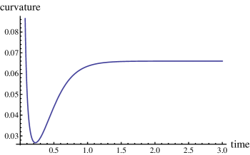
Figure 6.1. Example 1

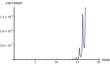
Figure 6.2. Example 2

7. Conclusion

The main result of this paper, Theorem 1.1, is proved. Firstly, through the analysis of higher curvatures of trajectories of systems, we give the relationship between curvatures of trajectories of two equivalent linear time-invariant systems. Secondly, for each type of real Jordan blocks, we analyze the relationship between the first curvature and stability. Finally, we prove a result for real Jordan canonical form, which completes the proof of the main theorem.

As Theorem 1.1 shows, two sufficient conditions for stability of the zero solution of linear time-invariant systems, based on the first curvature, are given. For each case of the theorem, we give an example to illustrate the result.

Further, we will investigate nonlinear control for the stability by using geometric description.

References

• [1] M. P. do Carmo, Differential Geometry of Curves and Surfaces, Prentice-Hall, 1976.
• [2] C.-T. Chen, Linear System Theory and Design, Third Edition, Oxford University Press, 1999.
• [3] H. Gluck, Higher Curvatures of Curves in Euclidean Space, American Mathematical Monthly, 73(1966), 699-704.
• [4] R. A. Horn and C. R. Johnson, Matrix Analysis, Second Edition, Cambridge University Press, 2013.
• [5] A. M. Lyapunov, The General Problem of the Stability of Motion (in Russian), Doctoral Dissertation, Univ. Kharkov, 1892.
• [6] J. E. Marsden, T. Ratiu and R. Abraham, Manifolds, Tensor Analysis, and Applications, Third Edition, Springer-Verlag, 2001.
• [7] L. Perko, Differential Equations and Dynamical Systems, Springer-Verlag, 1991.
• [8] Y. Wang, H. Sun, Y. Song, Y. Cao and S. Zhang, Description of Stability for Two and Three-Dimensional Linear Time-Invariant Systems Based on Curvature and Torsion, arXiv:1808.00290, August 1, 2018, preprint.