1 Introduction

Mathematical models of dynamical systems include physical or geometrical parameters, which are often affected by uncertainties. Thus the variability of the parameters has to be taken into account when using such models for predictive purposes. In parametric uncertainty quantification (UQ), the varying parameters are often replaced by random variables, see [27, 29]. The solutions of a dynamical system therefore become random processes, which encode the variability of the model output.

In this paper, we consider linear dynamical systems consisting of ordinary differential equations (ODEs) that have random input parameters. A time-dependent output is specified as a quantity of interest (QoI). Stochastic modelling via UQ yields a random QoI, which must be examined. Our main goal is to perform a sensitivity analysis of this random QoI with respect to the individual random parameters. One of the most popular approaches for this strategy, Sobol indices, is a technique for performing variance-based sensitivity analysis, see [20, 23, 24]. These sensitivity measures were employed to investigate dynamical systems in different applications, for example, a motor model [8], an epidemiological model [21] and a (discretised) heat equation [25]. Analysis via Sobol indices yields computationally tractable means of determining total effect sensitivity indices, which are defined by partial variances associated to each random parameter. Previous related work investigates the sensitivity of the transfer function associated to random ODEs in the frequency domain [14].

Our approach for computing sensitivities utilises polynomial chaos (PC) expansions; the random QoI is expanded into a separation-of-variables series, where each summand is the product of an orthogonal basis polynomial with a time-dependent coefficient function, see [28]. The stochastic Galerkin method with a PC ansatz yields a larger deterministic linear dynamical system, whose outputs are approximations to the time-dependent coefficients. In the previous work [16], the transfer function of the stochastic Galerkin system was examined componentwise to identify sparse approximations of the random QoI. We note that stochastic collocation approaches are likewise popular in parametric UQ settings, see [13], but analysis for collocation schemes is more difficult, so we restrict our attention to Galerkin methods.

We investigate system norms of the stochastic Galerkin method as sensitivity measures in the paper. Each partial variance can be written as a quadratic output of the stochastic Galerkin system. The first step in our approach transforms this system with a quadratic output into an equivalent linear dynamical system with multiple (linear) outputs. The norm of the output of these linear dynamical systems represents a single sensitivity coefficient for each random parameter. In particular, we investigate the Hankel norm and a Hardy norm of the systems in our analysis. The resulting sensitivity measures quantify the impact that each random parameter has on the random QoI, and upper bounds on this variability are derived. Thus the sensitivity analysis allows for the so-called screening, see [4], where random parameters with sufficiently low impact are detected and remodelled as constants to simplify the stochastic problem.

A major challenge in the above approach for sensitivity analysis is that the stochastic Galerkin dynamical system can be huge, and hence is computationally onerous to simulate. Our contribution is application of model order reduction (MOR) strategies to the high-dimensional stochastic Galerkin system, which results in a much smaller reduced-order model that is much easier to simulate. General information on MOR can be found in [1, 22]; in [15], the stochastic Galerkin method was reduced by a Krylov subspace method. In this paper, we use the technique of balanced truncation, where a-priori error bounds are available for the MOR. We provide analysis that bounds the proximity of the full-order model sensitivity measures and the reduced-order model sensitivity measures, so that our MOR approach is accompanied by a certifiable error estimate.

2 Random linear dynamical systems

We define the investigated problem in this section.

2.1 Linear dynamical systems

Let a time-invariant linear dynamical system be given in the form

$$\begin{split}E(p)\dot{x}(t,p)&=A(p)x(t,p)+B(p)u(t)\\[4.30554pt] y(t,p)&=C(p)x(t,p)\end{split}$$ (1)

for $t\geq 0$ with inputs $u:[0,\infty)\rightarrow\mathbbm{R}^{n_{\rm in}}$. The matrices $A,E\in\mathbbm{R}^{n\times n}$, $B\in\mathbbm{R}^{n\times n_{\rm in}}$, $C\in\mathbbm{R}^{n_{\rm out}\times n}$ depend on parameters $p\in\Pi\subseteq\mathbbm{R}^{q}$. We assume that the mass matrix $E$ is non-singular for all $p\in\Pi$, which implies a system of ODEs. Thus both the state variables $x:[0,\infty)\times\Pi\rightarrow\mathbbm{R}^{n}$ and the outputs $y:[0,\infty)\times\Pi\rightarrow\mathbbm{R}^{n_{\rm out}}$ are also parameter-dependent. Without loss of generality, we restrict the problem to a single output of the system ($n_{\rm out}=1$). Initial values

$$x(0,p)=x_{0}(p)$$ (2)

are predetermined by a function $x_{0}:\Pi\rightarrow\mathbbm{R}^{n}$. The state variables solving the initial value problem (1),(2) read as

$$x(t,p)={\rm e}^{E(p)^{-1}A(p)t}\left(x_{0}(p)+\int_{0}^{t}{\rm e}^{-E(p)^{-1}A(p)\tau}E(p)^{-1}B(p)u(\tau)\;{\rm d}\tau\right)$$ (3)

for $t\geq 0$ and each $p\in\Pi$ including the matrix exponential. However, this formula is not suitable for numerical evaluations.

Furthermore, we suppose that the system (1) is always asymptotically stable, i.e., all eigenvalues $\lambda\in\mathbbm{C}$ satisfying the condition

$$\det(\lambda E(p)-A(p))=0$$

have a negative real part for each $p\in\Pi$. Often the asymptotic stability of a model depends only on the topology of the underlying configuration and not on the values of the physical parameters, while still requiring positivity of some parameters. In [19, p. 124], the authors show a sufficient condition for linear electric circuits based on the topology. In [9], the asymptotic stability of a class of serial mass-spring-damper systems is proven.

2.2 Stochastic modelling

If the parameters are affected by uncertainties, then we use independent random variables on a probability space to model the parameter variations. The random variables are $p:\Omega\rightarrow\Pi$, $\omega\mapsto p(\omega)$ with an event space $\Omega$. Let a joint probability density function $\rho:\Pi\rightarrow\mathbbm{R}$ be given. If a measurable function $f:\Pi\rightarrow\mathbbm{R}$ depends on the parameters, then its expected value reads as

$$\mathbb{E}[f]=\int_{\Pi}f(p)\,\rho(p)\;{\rm d}p$$ (4)

provided that the integral is finite. The Hilbert space

$$\mathcal{L}^{2}(\Pi)=\left\{f:\Pi\rightarrow\mathbbm{R}\;:\;f\;\mbox{measurable and}\;\mathbb{E}[f^{2}]<\infty\right\}$$ (5)

is equipped with the inner product

$$\langle f,g\rangle=\int_{\Pi}f(p)g(p)\,\rho(p)\;{\rm d}p\qquad\mbox{for}\;\;f,g\in\mathcal{L}^{2}(\Pi).$$ (6)

The induced norm reads as $\|f\|_{\mathcal{L}^{2}(\Pi)}=\sqrt{\langle f,f\rangle}$. We assume that the matrices of the linear dynamical system (1) as well as the initial values (2) depend continuously on the parameters. The state variables are given by the formula (3). If the parameter domain $\Pi$ is compact, then the state variables $x(t,p)$ are uniformly bounded for all $p$ and fixed time $t$. It follows that the state variables are located in the Hilbert space (5) pointwise for each $t$. If the parameter domain $\Pi$ is infinite, then integrability conditions have to be satisfied to guarantee that the state variables belong to (5) pointwise in time. The output inherits the $\mathcal{L}^{2}(\Pi)$-property of the state variables if the matrix $C(p)$ is uniformly bounded for all $p\in\Pi$.

Let a complete orthonormal system $(\Phi_{i})_{i\in\mathbbm{N}}\subset\mathcal{L}^{2}(\Pi)$ consisting of polynomials be given, i.e.,

$$\langle\Phi_{i},\Phi_{j}\rangle=\left\{\begin{array}[]{ll}1&\mbox{for}\;i=j,\\ 0&\mbox{for}\;i\neq j.\\ \end{array}\right.$$

The theory of the generalised polynomial chaos (PC) implies a family of orthonormal polynomials for each traditional random distribution, see [29]. The multivariate polynomials are the products of univariate orthonormal polynomials. The total degree of a multivariate polynomial is the sum of the degrees in the univariate polynomials. Let the polynomials be ordered such that ${\rm degree}(\Phi_{i})\leq{\rm degree}(\Phi_{i+1})$ is satisfied. It follows that $\Phi_{1}$ is the unique constant polynomial.

Consequently, we expand the state variables as well as the output of the system (1) into

$$x(t,p)=\sum_{i=1}^{\infty}v_{i}(t)\Phi_{i}(p)\qquad\mbox{and}\qquad y(t,p)=\sum_{i=1}^{\infty}w_{i}(t)\Phi_{i}(p)$$ (7)

with coefficient functions $v_{i}:[0,\infty)\rightarrow\mathbbm{R}^{n}$ and $w_{i}:[0,\infty)\rightarrow\mathbbm{R}$. The series converge in the norm of the Hilbert space (5) and pointwise in time. The total variance of the random QoI becomes

$$V(t)=\sum_{i=2}^{\infty}w_{i}(t)^{2}$$ (8)

for each $t\geq 0$.

2.3 Stochastic Galerkin method

In a numerical approximation, we include all polynomials up to a total degree $d$ described by the set of integers

$$\mathcal{I}^{d}=\left\{i\in\mathbbm{N}\;:\;{\rm degree}(\Phi_{i})\leq d\right\}.$$ (9)

The cardinality is $|\mathcal{I}^{d}|=\frac{(d+q)!}{d!q!}$, see [29, p. 65]. Hence the infinite summation in (7) is restricted to

$$x^{(d)}(t,p)=\sum_{i\in\mathcal{I}^{d}}v_{i}(t)\Phi_{i}(p)\qquad\mbox{and}\qquad y^{(d)}(t,p)=\sum_{i\in\mathcal{I}^{d}}w_{i}(t)\Phi_{i}(p),$$ (10)

which represent truncated series. Inserting the approximations (10) into the linear dynamical system (1) yields a residual. The Galerkin approach requires the residual to be orthogonal to the space spanned by $\{\Phi_{i}:i\in\mathcal{I}^{d}\}$ with respect to the inner product (6). We obtain the larger linear system of ODEs

$$\begin{split}\hat{E}\dot{\hat{v}}(t)&=\hat{A}\hat{v}(t)+\hat{B}u(t)\\[4.30554pt] \hat{w}(t)&=\hat{C}\hat{v}(t)\end{split}$$ (11)

with state variables $\hat{v}:[0,\infty)\rightarrow\mathbbm{R}^{mn}$ and the same inputs $u$ as in (1). The system produces $m$ outputs $\hat{w}$ with $m=|\mathcal{I}^{d}|$, which represent approximations of the exact coefficient functions in (10). Let

$$S(p)=(\Phi_{i}(p)\Phi_{j}(p))_{i,j=1,\ldots,m}\quad\mbox{and}\quad s(p)=(\Phi_{i}(p))_{i=1,\ldots,m}$$

be auxiliary arrays. The definition of the matrices $\hat{A},\hat{E}\in\mathbbm{R}^{mn\times mn}$, $\hat{B}\in\mathbbm{R}^{mn\times n_{\rm in}}$, $\hat{C}\in\mathbbm{R}^{m\times mn}$ reads as

$$\hat{A}=\mathbb{E}[S\otimes A],\quad\hat{B}=\mathbb{E}[s\otimes B],\quad\hat{C}=\mathbb{E}[S\otimes C],\quad\hat{E}=\mathbb{E}[S\otimes E]$$ (12)

using Kronecker products, where the probabilistic integration (4) is applied componentwise. If the matrices $A,B,C,E$ consist of polynomials in the random variables, then the matrices (12) can be calculated analytically for traditional probability distributions. This property is an advantage in comparison to stochastic collocation techniques, where a quadrature error or sampling error emerges. More details on the stochastic Galerkin method for linear dynamical systems can be found in [15].

Initial values $\hat{v}(0)=\hat{v}_{0}$ have to be determined from the initial values (2) of the original system (1). If the initial values (2) are identical to zero, then the choice $\hat{v}(0)=0$ is obvious.

The stochastic Galerkin system (11) may be unstable even if all original systems (1) are asymptotically stable, see [18]. However, this loss of stability is rather seldom in practise. Thus we assume that the linear dynamical system (11) is asymptotically stable.

3 Sensitivity analysis

We investigate the sensitivity of the random output from the linear dynamical system (1) with respect to the individual random parameters. Local sensitivity measures are based on partial derivatives with respect to the parameters. Alternatively, we are interested in global variance-based sensitivity measures.

3.1 Partial variances and sensitivity indices

The Sobol indices provide a set of non-negative real numbers, which describe the interaction of each subset of random variables, see [23, 24]. Thus the number of Sobol indices is equal to the number of non-empty subsets, i.e., $2^{q}-1$. The Sobol indices yield the total effect sensitivity coefficients, which represent a variance-based sensitivity measure.

We consider an equivalent definition of the total effect sensitivity indices, which applies the PC expansion of a random-dependent function, cf. [26]. The random output of the system (1) exhibits the PC expansion (7). Let

$$\mathcal{I}_{j}=\left\{i\in\mathbbm{N}\;:\;\Phi_{i}\;\mbox{is non-constant in}\;p_{j}\right\}$$ (13)

be a set of integers for $j=1,\ldots,q$. Considering all polynomials up to a total degree $d$, we obtain the intersection of (9) and (13)

$$\mathcal{I}_{j}^{d}=\mathcal{I}_{j}\cap\mathcal{I}^{d}$$ (14)

for $j=1,\ldots,q$. The partial variance associated to the $j$th random variable becomes

$$V_{j}(t)=\sum_{i\in\mathcal{I}_{j}}w_{i}(t)^{2}$$ (15)

for $j=1,\ldots,q$ and each $t\geq 0$. It follows that $0\leq{V}_{j}(t)\leq{V}(t)$ for all $j$. We assume that the total variance (8) is positive for all $t>0$. (It would be a rare exception if the variance reduces exactly to zero at some positive time. In this case, variations of the QoI vanish and a UQ becomes obsolete.) The total effect sensitivity indices read as

$$S_{j}^{\rm T}(t)=\frac{V_{j}(t)}{V(t)}$$ (16)

for $j=1,\ldots,q$. It holds that $0\leq S_{j}^{\rm T}\leq 1$ for all $j$ and $1\leq S_{1}^{\rm T}+\cdots+S_{q}^{\rm T}\leq q$ pointwise in time. Often the sum of the sensitivity indices is close to one.

The stochastic Galerkin system (11) yields approximations of (16) by

$$\hat{S}_{j}^{\rm T}(t)=\frac{\hat{V}_{j}(t)}{\hat{V}(t)}$$ (17)

with

$$\hat{V}_{j}(t)=\sum_{i\in\mathcal{I}_{j}^{d}}\hat{w}_{i}(t)^{2}$$ (18)

using the outputs $\hat{w}_{1},\ldots,\hat{w}_{m}$ for the approximation of partial variances and, likewise, for the approximation $\hat{V}$ of the total variance (8).

In our context, the sensitivity indices (16) are time-dependent functions, which makes a sensitivity analysis more complicated. The choice of the input signals and the initial values determine these transient functions. Alternatively, we want to obtain a single number as sensitivity measure for each random variable, i.e., a finite set of $q$ non-negative coefficients.

3.2 Stochastic Galerkin system with quadratic outputs

Let $\hat{w}^{(j)}$ be the vector-valued function consisting of the components of $\hat{w}$ in $\mathcal{I}_{j}^{d}$ from (14). It follows that

$$\hat{V}_{j}(t)=\hat{w}^{(j)}(t)^{\top}\hat{w}^{(j)}(t)$$ (19)

for $j=1,\ldots,q$ due to (18). We arrange an own output matrix for this partial variance now. A square diagonal matrix is defined via

$$D_{j}={\rm diag}\left(d_{1}^{(j)},\ldots,d_{m}^{(j)}\right)\quad\mbox{with}\quad d_{\ell}^{(j)}=\left\{\begin{array}[]{rcl}1&\mbox{if}\;\ell\in\mathcal{I}_{j}^{d}\\ 0&\mbox{if}\;\ell\notin\mathcal{I}_{j}^{d}\\ \end{array}\right.$$

for each $j=1,\ldots,q$. The matrix-matrix product $\hat{C}_{j}^{\prime}=D_{j}\hat{C}$ replaces rows of $\hat{C}$ by zeros. The rank of $\hat{C}_{j}^{\prime}$ is $k=|\mathcal{I}_{j}^{d}|$, since the rank of $\hat{C}$ is $m$. We remove the rows identical to zero in $\hat{C}_{j}^{\prime}$ to obtain a condensed matrix $\hat{C}_{j}\in\mathbbm{R}^{k\times n}$. Observing (19), it follows that

$$\hat{V}_{j}(t)=\hat{w}^{(j)}(t)^{\top}\hat{w}^{(j)}(t)=\hat{v}(t)^{\top}\hat{C}_{j}^{\prime\top}\hat{C}_{j}^{\prime}\hat{v}(t)=\hat{v}(t)^{\top}\hat{C}_{j}^{\top}\hat{C}_{j}\hat{v}(t).$$ (20)

The partial variance of the $j$th random variable can be obtained from a stochastic Galerkin system

$$\begin{split}\hat{E}\dot{\hat{v}}(t)&=\hat{A}\hat{v}(t)+\hat{B}u(t)\\[4.30554pt] \hat{V}_{j}(t)&=\hat{v}(t)^{\top}\hat{C}_{j}^{\top}\hat{C}_{j}\hat{v}(t),\end{split}$$ (21)

where a single quadratic output is defined by the symmetric positive semi-definite matrix

$$M_{j}=\hat{C}_{j}^{\top}\hat{C}_{j}$$ (22)

for each $j=1,\ldots,q$.

Likewise, the total variance is given as the single quadratic output

$$\hat{V}(t)=\hat{v}(t)^{\top}\hat{C}^{\top}\hat{C}\hat{v}(t)$$

from the differential equations in the stochastic Galerkin system (11).

In [2, 3], the authors propose an approach for a general linear dynamical system with a quadratic output specified by a symmetric positive semi-definite matrix. A symmetric decomposition of this matrix is required like the (pivoted) Cholesky factorisation, for example. In our application, we already possess such a decomposition via (22). The alternative stochastic Galerkin systems

$$\begin{split}\hat{E}\dot{\hat{v}}(t)&=\hat{A}\hat{v}(t)+\hat{B}u(t)\\[4.30554pt] \hat{z}_{j}(t)&=\hat{C}_{j}\hat{v}(t)\end{split}$$ (23)

are arranged for $j=1,\ldots,q$ with multiple outputs ($n_{\rm out}=k=|\mathcal{I}_{j}^{d}|$). It holds that $\hat{V}_{j}=\hat{z}_{j}^{\top}\hat{z}_{j}$ for the quadratic output of (21) due to (20).

3.3 System norms

Given a vector-valued function $x\in\mathcal{L}^{2}([0,\infty))^{n}$ with $n$ components, its signal norm reads as

$$\|x\|_{\mathcal{L}^{2}([0,\infty))}=\sqrt{\int_{0}^{\infty}x(t)^{\top}x(t)\;{\rm d}t}\,.$$

Several norms are defined for a general linear dynamical system. Let $\hat{\Sigma}$ and $\hat{\Sigma}_{1},\ldots,\hat{\Sigma}_{q}$ represent the stochastic Galerkin systems (11) and (23), respectively. The Hankel norm denotes a bound on the signal norm of future outputs generated by inputs in the past (input is zero for $t\geq 0$). This norm exhibits the formula, cf. [1, p. 135],

$$\|\hat{\Sigma}\|_{\rm H}=\sup\left\{\frac{\|\hat{w}\|_{\mathcal{L}^{2}([0,\infty))}}{\|u\|_{\mathcal{L}^{2}((-\infty,0])}}\;:\;u\in\mathcal{L}^{2}((-\infty,0])^{n_{\rm in}},\;u\neq 0\right\}.$$ (24)

In addition, the Hankel norm is equal to the maximum Hankel singular value of the system, which will be specified in Section 4.1. The system norm directly describes the mapping from inputs to outputs provided that the initial values are zero, i.e.,

$$\|\hat{\Sigma}\|_{\mathcal{L}^{2}}=\sup\left\{\frac{\|\hat{w}\|_{\mathcal{L}^{2}([0,\infty))}}{\|u\|_{\mathcal{L}^{2}([0,\infty))}}\;:\;u\in\mathcal{L}^{2}([0,\infty))^{n_{\rm in}},\;u\neq 0,\;\hat{v}(0)=0\right\}.$$ (25)

Let $\hat{G}:\mathbbm{C}\backslash\Xi\rightarrow\mathbbm{C}^{m\times n_{\rm in}}$ be the transfer function of the stochastic Galerkin system (11) in the frequency domain. Therein, $\Xi\subset\mathbbm{C}$ is a finite set of poles. The magnitude of a transfer function can be characterised by the Hardy norms $\|\cdot\|_{\mathcal{H}_{2}}$ and $\|\cdot\|_{\mathcal{H}_{\infty}}$. The $\mathcal{H}_{\infty}$-norm of a transfer function coincides with its $\mathcal{L}^{\infty}$-norm, which is a frequency domain Lebesgue norm, provided that the system is asymptotically stable. It follows that, see [1, p. 149],

$$\|\hat{G}\|_{\mathcal{H}_{\infty}}=\sup_{\omega\in\mathbbm{R}}\;\sigma_{\max}(\hat{G}({\rm i}\omega)),$$ (26)

where $\sigma_{\max}$ is the maximum singular value of the matrix-valued transfer function and ${\rm i}=\sqrt{-1}$. The norms satisfy the relations

$$\|\hat{\Sigma}\|_{\rm H}\leq\|\hat{\Sigma}\|_{\mathcal{L}^{2}}=\|\hat{G}\|_{\mathcal{H}_{\infty}},$$ (27)

which are valid for any asymptotically stable system of ODEs.

3.4 Sensitivity measures

We use the norms of the stochastic Galerkin systems (23) from Section 3.3 to indicate the sensitivity of the random output in the original system (1). In contrast, the $\mathcal{H}_{2}$-norms and $\mathcal{H}_{\infty}$-norms of the separate components of the transfer function $\hat{G}$ were analysed to identify a sparse representation of the random output in [16].

The following two definitions introduce the key data in our investigations.

Definition 1

The sensitivity coefficients $\hat{\eta}_{j}$ are the real values

$$\hat{\eta}_{j}=\|\hat{\Sigma}_{j}\|_{\rm H}$$ (28)

for $j=1,\ldots,q$ using the Hankel norms (24) of the stochastic Galerkin systems (23).

Definition 2

The sensitivity coefficients $\hat{\theta}_{j}$ are the real values

$$\hat{\theta}_{j}=\|\hat{\Sigma}_{j}\|_{\mathcal{L}^{2}}=\|\hat{G}_{j}\|_{\mathcal{H}_{\infty}}$$ (29)

for $j=1,\ldots,q$ using the system norms (25) of the stochastic Galerkin systems (23).

The general relation (27) shows that

$$\hat{\eta}_{j}\leq\hat{\theta}_{j}\qquad\mbox{for each}\;\;j=1,\ldots,q.$$ (30)

The sensitivity measure (29) is more important than (28), because (28) does not directly relate to the input-output mapping for $t\geq 0$. However, the computation of an $\mathcal{H}_{\infty}$-norm is more costly than the calculation of a Hankel norm. We obtain an inequality between the system norms of the Galerkin system (11) and the modified Galerkin systems (23).

Lemma 1

Let $\hat{\Sigma}$ and $\hat{\Sigma}_{1},\ldots,\hat{\Sigma}_{q}$ represent the linear dynamical systems (11) and (23), respectively. It holds that $\|\hat{\Sigma}_{j}\|_{\mathcal{L}^{2}}\leq\|\hat{\Sigma}\|_{\mathcal{L}^{2}}$ for $j=1,\ldots,q$ in the system norm (25).

Proof:

The outputs of the system (11) and the systems (23) are $\hat{w}$ and $\hat{z}_{1},\ldots,\hat{z}_{q}$, respectively. We obtain the estimate

$$\|\hat{w}\|_{\mathcal{L}^{2}([0,\infty))}^{2} =\int_{0}^{\infty}\sum_{i\in\mathcal{I}^{d}}\hat{w}_{i}(t)^{2}\;{\rm d}t\geq\int_{0}^{\infty}\sum_{i\in\mathcal{I}_{j}^{d}}\hat{w}_{i}(t)^{2}\;{\rm d}t=\int_{0}^{\infty}\hat{z}_{j}(t)^{\top}\hat{z}_{j}(t)\;{\rm d}t$$

$$=\|\hat{z}_{j}\|_{\mathcal{L}^{2}([0,\infty))}^{2}$$

for $j=1,\ldots,q$. It follows that $\|\hat{z}_{j}\|_{\mathcal{L}^{2}([0,\infty))}\leq\|\hat{w}\|_{\mathcal{L}^{2}([0,\infty))}$ if the same input is supplied to all systems. Observing (25), we arrange the supremum and achieve the statement. $\Box$

We show a bound on the norm of partial variances in the time domain, which yields an interpretation of the sensitivity measure in Definition 2.

Lemma 2

The stochastic Galerkin systems (23) with initial values zero yield approximations of the partial variances, which satisfy the bounds

$$\|\hat{V}_{j}\|_{\mathcal{L}^{1}([0,\infty))}\leq\hat{\theta}_{j}^{2}\,\|u\|_{\mathcal{L}^{2}([0,\infty))}^{2}$$

for $j=1,\ldots,q$ including the sensitivity coefficients (29).

Proof:

We obtain

$$\|\hat{V}_{j}\|_{\mathcal{L}^{1}[0,\infty)} =\int_{0}^{\infty}\hat{V}_{j}(t)\;{\rm d}t=\int_{0}^{\infty}\hat{z}_{j}(t)^{\top}\hat{z}_{j}(t)\;{\rm d}t=\|\hat{z}_{j}\|_{\mathcal{L}^{2}([0,\infty))}^{2}$$

$$\leq\|\hat{\Sigma}_{j}\|_{\mathcal{L}^{2}}^{2}\|u\|_{\mathcal{L}^{2}([0,\infty))}^{2}=\hat{\theta}_{j}^{2}\|u\|_{\mathcal{L}^{2}([0,\infty))}^{2}$$

due to (25) and (29). $\Box$

The definition of the total effect sensitivity indices (16) motivates to establish relative sensitivity measures

$$\hat{\eta}_{j}^{\rm rel}=\frac{\|\hat{\Sigma}_{j}\|_{\rm H}}{\|\hat{\Sigma}\|_{\rm H}}\qquad\mbox{as well as}\qquad\hat{\theta}_{j}^{\rm rel}=\frac{\|\hat{\Sigma}_{j}\|_{\mathcal{L}^{2}}}{\|\hat{\Sigma}\|_{\mathcal{L}^{2}}}$$

for $j=1,\ldots,q$. Lemma 1 guarantees $\hat{\theta}_{j}^{\rm rel}\leq 1$, whereas $\hat{\eta}_{j}^{\rm rel}$ may be larger than one. However, since the denominators are identical for $j=1,\ldots,q$, we can investigate the normalised quantities

$$\hat{\eta}_{j}^{*} =\frac{\hat{\eta}_{j}}{\hat{\eta}_{1}+\cdots+\hat{\eta}_{q}},$$ (31)

$$\hat{\theta}_{j}^{*} =\frac{\hat{\theta}_{j}}{\hat{\theta}_{1}+\cdots+\hat{\theta}_{q}}$$ (32)

as well. Now it holds that $0\leq\hat{\eta}_{j}^{*},\hat{\theta}_{j}^{*}\leq 1$ for all $j=1,\ldots,q$.

3.5 Error bound in screening

The sensitivity measures identify the random variables with high impact and low impact. Random variables with low impact can be remodelled by constants to decrease the dimensionality of the random parameter space. This strategy is called screening, see [4], or freezing of unessential random variables, see [23]. We derive a bound on the error of this screening.

Theorem 1

Let the random variables be partitioned into $p=(a,b)$ with $a\in\Pi_{a}\subseteq\mathbbm{R}^{q^{\prime}}$, $b\in\Pi_{b}\subseteq\mathbbm{R}^{q-q^{\prime}}$. Let $\bar{y}(t,p)=y(t,a,\bar{b})$ with a constant $\bar{b}\in\Pi_{b}$. For each $\delta\in(0,1)$, there is a set $B_{\delta}\subset\Pi_{b}$ of probability larger $1-\delta$ such that

$$\left\|y-\bar{y}\right\|_{\mathcal{L}^{2}(\Pi\times[0,\infty))}^{2}<\left(1+{\textstyle\frac{1}{\delta}}\right)\sum_{j=q^{\prime}+1}^{q}\|V_{j}\|_{\mathcal{L}^{1}([0,\infty))}$$

for all $\bar{b}\in B_{\delta}$ in the norm of the product space $\Pi\times[0,\infty)$.

Proof:

The analysis in [23] shows that

$$\int_{\Pi}\left(y(t,a,b)-y(t,a,\bar{b})\right)^{2}\rho(p)\;{\rm d}p<\left(1+{\textstyle\frac{1}{\delta}}\right)\sum_{j=q^{\prime}+1}^{q}V_{j}(t)$$

pointwise for each $t\geq 0$. Time integration in $[0,\infty)$ yields

$$\left\|y-\bar{y}\right\|_{\mathcal{L}^{2}(\Pi\times[0,\infty))}^{2} =\int_{0}^{\infty}\int_{\Pi}\left(y(t,p)-\bar{y}(t,p)\right)^{2}\rho(p)\;{\rm d}p\;{\rm d}t$$

$$<\left(1+{\textstyle\frac{1}{\delta}}\right)\int_{0}^{\infty}\sum_{j=q^{\prime}+1}^{q}V_{j}(t)\;{\rm d}t=\left(1+{\textstyle\frac{1}{\delta}}\right)\sum_{j=q^{\prime}+1}^{q}\|V_{j}\|_{\mathcal{L}^{1}([0,\infty))},$$

because the partial variances are non-negative. $\Box$

The stochastic Galerkin systems generate approximations of the partial variances (15). Assuming that $\hat{V}_{j}-V_{j}$ is sufficiently small for $j=q^{\prime}+1,\ldots,q$, Lemma 2 and Theorem 1 imply the approximate bound

$$\left\|y-\bar{y}\right\|_{\mathcal{L}^{2}(\Pi\times[0,\infty))}<\sqrt{{\textstyle\left(1+\frac{1}{\delta}\right)}\sum_{j=q^{\prime}+1}^{q}\hat{\theta}_{j}^{2}\;\mbox{}}\;\|u\|_{\mathcal{L}^{2}([0,\infty))}.$$

This inequality shows that the random variables $b$ can be replaced by constants if the associated sensitivity measures (29) are sufficiently small.

4 Model order reduction

We examine the potential for a cheap computation of the sensitivity measures in Definition 1 and Definition 2 using methods of MOR.

4.1 Balanced truncation

We apply an MOR to the stochastic Galerkin system (11) using the technique of balanced truncation, see [1]. This MOR method is applicable to all asymptotically stable linear systems of ODEs. The controllability Gramian $P$ and the observability Gramian $Q$ are given by the solutions of the Lyapunov equations

$$\hat{A}P\hat{E}^{\top}+\hat{E}P\hat{A}^{\top}+\hat{B}\hat{B}^{\top} =0,$$ (33)

$$\hat{A}^{\top}Q\hat{E}+\hat{E}^{\top}Q\hat{A}+\hat{C}^{\top}\hat{C} =0.$$ (34)

We require symmetric decompositions $P=L_{P}{L_{P}}^{\top}$ and $Q=L_{Q}{L_{Q}}^{\top}$. For example, the Cholesky factorisation can be directly computed without solving for $P$ or $Q$ first, see [7]. The singular value decomposition (SVD)

$$U_{\rm l}S{U_{\rm r}}^{\top}={L_{Q}}^{\top}\hat{E}L_{P}$$ (35)

is calculated with a diagonal matrix $S={\rm diag}(\sigma_{1},\ldots,\sigma_{mn})$ and orthogonal matrices $U_{\rm l},U_{\rm r}\in\mathbbm{R}^{mn\times mn}$. The diagonal matrix includes the Hankel singular values in descending order ($\sigma_{\ell}\geq\sigma_{\ell+1}$).

Any reduced dimension $r<mn$ can be chosen. Let $\tilde{S}\in\mathbbm{R}^{r\times r}$ be the diagonal matrix including the $r$ largest singular values. Let $\tilde{U}_{\rm l},\tilde{U}_{\rm r}\in\mathbbm{R}^{mn\times r}$ be the matrices consisting of first $r$ columns in $U_{\rm l},U_{\rm r}$. We obtain projection matrices $T_{\rm l},T_{\rm r}\in\mathbbm{R}^{mn\times r}$ of full (column) rank by

$$T_{\rm l}=L_{Q}\tilde{U}_{\rm l}\tilde{S}^{-\frac{1}{2}}\qquad\mbox{and}\qquad T_{\rm r}=L_{P}\tilde{U}_{\rm r}\tilde{S}^{-\frac{1}{2}}.$$

Alternatively, just the $r$ dominant singular values and their singular vectors have to be computed to obtain these projection matrices.

The reduced matrices read as

$$\tilde{A}=T_{\rm l}^{\top}\hat{A}T_{\rm r},\quad\tilde{B}=T_{\rm l}^{\top}\hat{B},\quad\tilde{C}=\hat{C}T_{\rm r},\quad\tilde{E}=T_{\rm l}^{\top}\hat{E}T_{\rm r}.$$ (36)

The matrices produce a linear dynamical system of the same form but smaller dimension $r$. The reduced mass matrix $\tilde{E}$ is non-singular. Let $\tilde{w}$ be its multiple output, where the number of outputs is still $m$.

We use the same projection matrices for reductions of the linear dynamical systems (23). Just the matrices

$$\tilde{C}_{j}=\hat{C}_{j}T_{\rm r}$$

are changed for $j=1,\ldots,q$. Moreover, the balanced truncation technique guarantees that each reduced-order model (ROM) inherits the asymptotic stability of the full-order model (FOM).

Direct methods of linear algebra yield the numerical solution of the Lyapunov equations (33),(34), see [7]. Alternatively, approximate methods or iteration schemes are available like Krylov subspace techniques and the alternating direction implicit (ADI) method, see [6]. Such methods produce low-rank approximations of the Cholesky factors. However, the efficiency is often critical if the matrices $\hat{B}$ or $\hat{C}$ exhibit a high rank. The number of inputs typically satisfies $n_{\rm in}<n\ll mn$ and (33) can be solved efficiently. In contrast, it holds that ${\rm rank}(\hat{C})=m$ and thus the rank is relatively large for moderate $n$, where the approximate solution of (34) becomes critical.

4.2 Error bound for sensitivity measures

We show an a-priori error bound on our sensitivity measures from Definition 1 and Definition 2.

Theorem 2

Let $\hat{\Sigma}_{j}$ be the linear stochastic Galerkin system (23) and $\tilde{\Sigma}_{j}$ be its ROM of dimension $r$ obtained by balanced truncation of the complete stochastic Galerkin system (11). The error of the sensitivity measures (28) and (29) satisfy the bound

$$\max\left\{\big{|}\hat{\eta}_{j}-\tilde{\eta}_{j}\big{|},\big{|}\hat{\theta}_{j}-\tilde{\theta}_{j}\big{|}\right\}\leq 2\sum_{k=r+1}^{mn}\sigma_{k}$$ (37)

uniformly for all $j=1,\ldots,q$. The Hankel singular values $\sigma_{1}\geq\sigma_{2}\geq\cdots\geq\sigma_{mn}$ belong to the stochastic Galerkin system (11).

Proof:

It holds that $\hat{\eta}_{j}=\|\hat{\Sigma}_{j}\|_{\rm H}$, $\hat{\theta}_{j}=\|\hat{\Sigma}_{j}\|_{\mathcal{L}^{2}}$ and $\tilde{\eta}_{j}=\|\tilde{\Sigma}_{j}\|_{\rm H}$, $\tilde{\theta}_{j}=\|\tilde{\Sigma}_{j}\|_{\mathcal{L}^{2}}$ for the sensitivity measures from FOM and ROM, respectively. The reverse triangle inequality of the norms yields

$$\big{|}\hat{\eta}_{j}-\tilde{\eta}_{j}\big{|} =\left|\|\hat{\Sigma}_{j}\|_{\rm H}-\|\tilde{\Sigma}_{j}\|_{\rm H}\right|\leq\left\|\hat{\Sigma}_{j}-\tilde{\Sigma}_{j}\right\|_{\rm H},$$

$$\big{|}\hat{\theta}_{j}-\tilde{\theta}_{j}\big{|} =\left|\|\hat{\Sigma}_{j}\|_{\mathcal{L}^{2}}-\|\tilde{\Sigma}_{j}\|_{\mathcal{L}^{2}}\right|\leq\left\|\hat{\Sigma}_{j}-\tilde{\Sigma}_{j}\right\|_{\mathcal{L}^{2}}.$$

Let $\hat{G}$ and $\tilde{G}$ denote the transfer functions of FOM and ROM, respectively. Lemma 1 together with the general relation (27) show that

$$\left\|\hat{\Sigma}_{j}-\tilde{\Sigma}_{j}\right\|_{\rm H}\leq\left\|\hat{\Sigma}_{j}-\tilde{\Sigma}_{j}\right\|_{\mathcal{L}^{2}}\leq\left\|\hat{\Sigma}-\tilde{\Sigma}\right\|_{\mathcal{L}^{2}}=\left\|\hat{G}-\tilde{G}\right\|_{\mathcal{H}_{\infty}}$$

uniformly for $j=1,\ldots,q$, because the involved systems are asymptotically stable. Using balanced truncation, the error estimate

$$\left\|\hat{G}-\tilde{G}\right\|_{\mathcal{H}_{\infty}}\leq 2\sum_{k=r+1}^{mn}\sigma_{k}$$

holds true in the $\mathcal{H}_{\infty}$-norm (26), see [1, p. 212]. $\Box$

Theorem 2 demonstrates that the approximation of the sensitivity measures inherits the error bound of the balanced truncation MOR.

5 Illustrative example

We apply the sensitivity analysis from Section 3 to a test example now. We computed on a FUJITSU Esprimo P920 Intel(R) Core(TM) i5-4570 CPU with 3.20 GHz (4 cores) and operation system Microsoft Windows 7. The software package MATLAB [12] (version R2018a) was used for all computations.

5.1 Mass-spring-damper system

A general linear mass-spring-damper configuration is described by a second-order system of ODEs

$$M\ddot{z}(t)+D\dot{z}(t)+Kz(t)=f(t)$$ (38)

for the positions $z:[0,\infty)\rightarrow\mathbbm{R}^{\ell}$ with mass matrix $M$, damping matrix $D$, stiffness matrix $K$ and an excitation $f:[0,\infty)\rightarrow\mathbbm{R}^{\ell}$.

We examine a mass-spring-damper system introduced in [11], which is depicted in Figure 1. This mechanical configuration incorporates $q=14$ positive physical parameters: 4 masses, 6 spring constants and 4 damping constants. The single input is an excitation at the bottom spring, whereas the single output is the position of the top mass. The mathematical modelling yields the symmetric matrices $M={\rm diag}(m_{1},m_{2},m_{3},m_{4})$,

$$D=\begin{pmatrix}d_{1}&-d_{1}&0&0\\ -d_{1}&d_{1}+d_{2}&-d_{2}&0\\ 0&-d_{2}&d_{2}+d_{3}&-d_{3}\\ 0&0&-d_{3}&d_{3}+d_{4}\\ \end{pmatrix},$$

$$K=\begin{pmatrix}k_{1}+k_{2}+k_{5}&-k_{2}&0&-k_{5}\\ -k_{2}&k_{2}+k_{3}&-k_{3}&0\\ 0&-k_{3}&k_{3}+k_{4}&-k_{4}\\ -k_{5}&0&-k_{4}&k_{4}+k_{5}+k_{6}\\ \end{pmatrix}$$

together with the excitation $f(t)=(k_{1}u(t),0,0,0)^{\top}$. Obviously, if all parameters are positive, then $M$ is positive definite and $D$ as well as $K$ are positive semi-definite. A symbolic Cholesky decomposition is possible for both $D$ and $K$. Thus these matrices are also positive definite. It follows that the linear dynamical system is always asymptotically stable, see [10, p. 103].

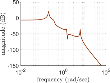
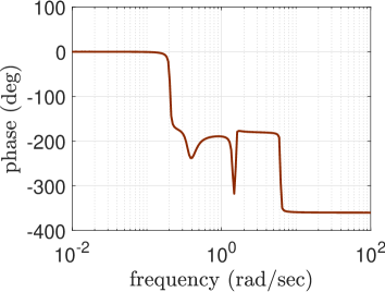
The system (38) is transformed into an equivalent first-order system (1) with dimension $n=8$. Figure 2 shows the Bode plot of the linear dynamical system in the case of a constant choice of the parameters from [11], i.e., $m_{1}=1$, $m_{2}=5$, $m_{3}=25$, $m_{4}=125$, $k_{1}=27$, $k_{2}=9$, $k_{3}=3$, $k_{4}=1$, $k_{5}=2$, $k_{6}=3$, $d_{1}=0.1$, $d_{2}=0.4$, $d_{3}=1.6$, $d_{4}=1$. This test example was also investigated in [16, 17].

Figure 1: Mass-spring-damper configuration.

Figure 2: Bode plot of mass-spring-damper system for deterministic parameters.

5.2 Stochastic modelling and Galerkin method

We replace the parameters by independent random variables with uniform probability distributions, which vary 10% around the used constant choice of the parameters. Consequently, the PC expansions (7) include the (multivariate) Legendre polynomials. We arrange finite sums (10) with all polynomials up to total degree $d=3$. The stochastic Galerkin system (11) exhibits the state space dimension $mn=5440$ and the number of outputs becomes $m=680$. The matrices of the Galerkin system can be computed analytically, because the entries of matrices in the underlying system (38) are linear functions of the physical parameters. Hence we calculate these matrices exactly except for round-off errors. Furthermore, the stochastic Galerkin system is asymptotically stable, because the maximum real part of the associated eigenvalues is computed to $-0.0048$ and thus negative.

5.3 Numerical results for sensitivity measures

We computed all Hankel norms by direct methods of linear algebra. In contrast, the $\mathcal{H}_{\infty}$-norm could only be calculated by approximation. We did not determine the $\mathcal{H}_{\infty}$-norm of the system (11), because the computational effort would be too large due to the high dimensionality.

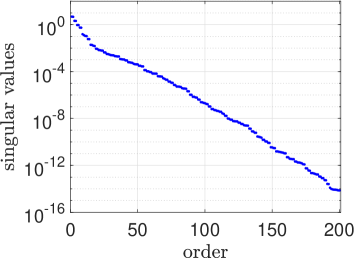
We generate ROMs of the FOM (11) by the balanced truncation technique from Section 4.1. A direct method of linear algebra yields the Cholesky factors of the solutions satisfying the Lyapunov equations (33),(34). More details on the numerical method are given in the following subsection. Figure 3 illustrates the dominant Hankel singular values in the decomposition (35). The largest Hankel singular value coincides with the Hankel norm $\|\hat{\Sigma}\|_{\rm H}=4.84$.

Figure 3: Hankel singular values of the stochastic Galerkin system (11) for the mass-spring-damper example.

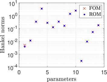
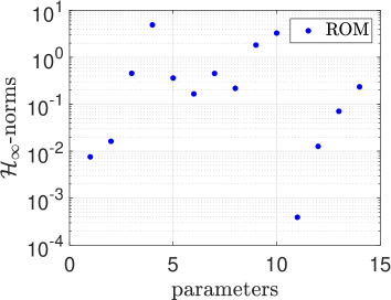
Now we analyse the sensitivities. On the one hand, the FOMs (23) yield the sensitivity measures (28). On the other hand, the ROMs of dimension $r=25$ produce approximations of the sensitivity coefficients (28) as well as (29). Figure 4 depicts the results, which demonstrate a good agreement between the sensitivity measures from FOM and ROM. Concerning the inequality (30), the $\mathcal{H}_{\infty}$-norms are just slightly larger than the Hankel norms. Furthermore, the system norm of the ROM for the stochastic Galerkin method (11) is $\|\tilde{\Sigma}\|_{\mathcal{L}^{2}}=\|\tilde{G}\|_{\mathcal{H}_{\infty}}=7.75$.

Figure 4: Sensitivity coefficients (28) from Hankel norms (left) and sensitivity coefficients (29) from Hardy norms (right) with respect to the random parameters (1-4: masses, 5-10: springs, 11-14: dampers).

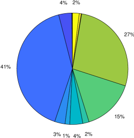
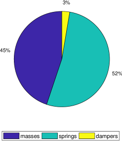
The sensitivities indicate the impact of the random parameters on the random QoI. The normalised sensitivity measures (32) are illustrated by Figure 5 (left). We observe that three parameters are dominant, which are the top mass, the spring above the top mass and the spring connecting bottom mass and top mass, cf. Figure 1. In contrast, five parameters exhibit a contribution less than 1%. Thus these parameters can be remodelled by constants to reduce the dimension of the random space. Furthermore, Figure 5 (right) shows the sum of the normalised sensitivity measures (32) for the three different types of parameters. We recognise that the dampers feature a relatively low impact on the random QoI.

Figure 5: Normalised sensitivity measures (32) for the random parameters (left) and merged normalised sensitivity measures for the three groups of physical parameters (right).

5.4 Comparison of MOR methods

We compare the error between FOM and ROM for the computed sensitivity measures (28). The error indicator is defined as

$$\max_{j=1,\ldots,q}\left|\hat{\eta}_{j}-\tilde{\eta}_{j}\right|.$$ (39)

We do not consider the errors of the sensitivity measures (29), because the computation work for the system norms of the FOMs (23) is too high to be performed on our computer.

The following three variants of MOR methods are applied in MATLAB:

• Balanced truncation with direct solution of the Lyapunov equations using the function lyapchol of the control system toolbox. In the direct method, we use the matrices $\hat{A}^{\prime}=\hat{E}^{-1}\hat{A}$, $\hat{B}^{\prime}=\hat{E}^{-1}\hat{B}$ and $\hat{E}^{\prime}=I$ (identity) to simplify the Lyapunov equations, because the numerical solution becomes significantly faster. These matrices can be computed with negligible effort by a sparse $LU$-decomposition of $\hat{E}$.

• Balanced truncation with iterative solution of the Lyapunov equations by the ADI method using the function lyapchol of the sss toolbox, see [5]. The iteration performs until a default tolerance is achieved, which yields approximate factors of rank 301.

• One-sided Arnoldi method, see [1, p. 334], with a single real expansion point $s_{0}=0$. The projection matrix $T_{\rm r}$ is determined by the matrices $\hat{A},\hat{B},\hat{E}$ of (11) and thus this approach is independent of the definition of outputs. It holds that $T_{\rm l}=T_{\rm r}$ used in (36).

In each technique, we calculate projection matrices $T_{\rm l},T_{\rm r}$ of rank $r_{\max}=100$. We extract the leading columns of the projection matrices to obtain ROMs of dimensions $r=5,10,15,\ldots,100$. Furthermore, the method (i) yields all Hankel singular values in the decomposition (35).

Figure 6 (left) shows the maximum error (39) for the techniques (i) and (ii). Therein, the error bound (37) obtained by Theorem 2 is also depicted. In the direct method (i), the true error is much below the predicted error bound. The approximate method (ii) produces significantly higher errors in comparison to the direct method, which indicates a critical behaviour due to the large number of outputs in the system (11). Nevertheless, the accuracy becomes better for increasing dimensions of the ROMs. Figure 6 (right) displays the maximum error (39) for the technique (iii). This error is larger for reduced dimensions $r\geq 50$ in comparison to (i) and (ii). Furthermore, the accuracy does not improve any more for dimensions $r\geq 100$ in the Arnoldi method. This is a well-known phenomenon due to the accumulation of round-off errors in the orthogonalisation procedure. Moreover, there is no prior or posterior error bound for the Arnoldi method.

Figure 6: Errors (39) for different reduced dimensions in balanced truncation techniques (left) and Arnoldi method (right).

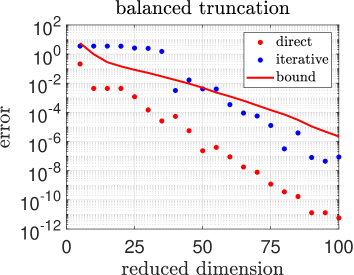
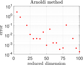
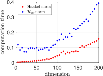
Table 1 provides the computation times, which represent elapsed real times in seconds, of the balanced truncation techniques. Only the $r_{\max}$ dominant singular values and their singular vectors are computed in the SVD (35) now. The Arnoldi method requires a computation time of only 1.3 seconds for the projection matrix of rank $r_{\max}$. Furthermore, the computation times for a single Hankel norm and a single system norm of an ROM are illustrated by Figure 7. In this case, we use the direct method (i) to arrange ROMs up to dimension $r=200$. Yet the computational effort depends mainly on the reduced dimension and not on the used MOR method. The work has to be done for each random variable, i.e., $q$ times. We recognise that this computation time is small in comparison to the construction of the ROMs by balanced truncation techniques.

Table 1: Computation times in seconds within balanced truncation MOR.

	direct method	ADI method
Lyapunov equation (33)	467	–
Lyapunov equation (34)	695	–
both Lyapunov equations	1162	26
singular value decomposition (35)	19	0.3

Figure 7: Computation times in seconds for a Hankel norm and a $\mathcal{H}_{\infty}$-norm depending on the dimension of a linear dynamical system with dense matrices.

The comparison demonstrates that there is a trade-off between accuracy and computational effort in the MOR methods. The balanced truncation using a direct solver is expensive, whereas an a-priori error bound is guaranteed. The direct method is still much cheaper than a computation of the system norms for the FOMs (23).

5.5 Transient simulation

Finally, we perform a transient simulation of the Galerkin system (11) for $t\in[0,1000]$ with initial values zero. The chirp signal

$$u(t)=\sin\left(\textstyle\frac{t^{2}}{10}\right)$$

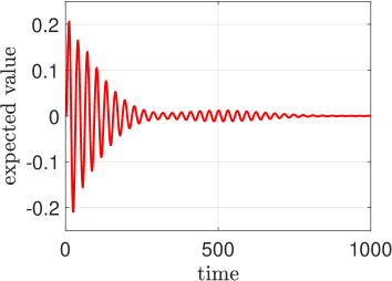
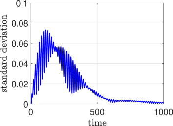
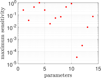
is supplied, which runs through a continuum of frequencies. We use the trapezoidal rule in the time integration. Figure 8 depicts the approximations of the expected value and the standard deviation for the random QoI. We compute the approximations (17) of the total effect sensitivity indices (16) for each random variable. Concerning the discrete time points, the maximum values are illustrated by Figure 9. The relative positions of the sensitivity indices are similar to the sensitivity measures (28),(29) shown in Figure 4.

Figure 8: Expected value (left) and standard deviation (right) of random output in transient simulation of mass-spring-damper system.

Figure 9: Maximum in time of total effect sensitivity indices (17) with respect to the random parameters (1-4: masses, 5-10: springs, 11-14: dampers).

References

- [1] A. Antoulas, Approximation of Large-Scale Dynamical Systems, SIAM Publications, 2005.
- [2] R. Van Beeumen, K. Meerbergen, Model reduction by balanced truncation of linear systems with a quadratic output, in: T.E. Simons, G. Psihoyios, Ch. Tsitouras (eds.), International Conference on Numerical Analysis and Applied Mathematics (ICNAAM), 2010, pp. 2033–2036.
- [3] R. Van Beeumen, K. Van Nimmen, G. Lombaert, K. Meerbergen, Model reduction for dynamical systems with quadratic output, Int. J. Numer. Meth. Engng. 91 (2012) 229-–248.
- [4] F. Campolongo, J. Cariboni, A. Saltelli, An effective screening design for sensitivity analysis of large models, Environmental Modelling & Software 22 (2007) 1509–1518.
- [5] A. Castagnotto, M. Cruz Varona, L. Jeschek, B. Lohmann, sss & sssMOR: Analysis and reduction of large-scale dynamic systems in MATLAB, Automatisierungstechnik 65 (2017) 134–150.
- [6] V. Druskin, L. Knizhnerman, V. Simoncini, Analysis of the rational Krylov subspace and ADI methods for solving the Lyapunov equation, SIAM J. Numer. Anal. 49 (2011) 1875–1898.
- [7] S.J. Hammarling, Numerical solution of stable non-negative definite Lyapunov equation, IMA J. Numer. Anal. 2 (1982) 303–323.
- [8] E. Haro Sandoval, F. Anstett-Collin, M. Basset, Sensitivity study of dynamic systems with polynomial chaos, Reliability Engineering & System Safety 104 (2012) 15–26.
- [9] J.B. Hoagg, J. Chandrasekar, D.S. Bernstein, On the zeros, initial undershoot, and relative degree of collinear lumped-parameter structures, ASME J. Dyn. Sys. Meas. Contr. 129 (2007) 493–502.
- [10] D.J. Inman, Vibration and Control, John Wiley & Sons, Ltd, 2006.
- [11] B. Lohmann, R. Eid, Efficient order reduction of parametric and nonlinear models by superposition of locally reduced models, in: G. Roppenecker, B. Lohmann (eds.), Methoden und Anwendungen der Regelungstechnik, Shaker, 2009.
- [12] MATLAB, version 9.4.0.813654 (R2018a), The Mathworks Inc., Natick, Massachusetts, 2018.
- [13] A. Narayan, T. Zhou, Stochastic collocation on unstructured multivariate meshes, Comm. Comput. Phys. 18 (2015) 1–36.
- [14] R. Pulch, E.J.W. ter Maten, F. Augustin, Sensitivity analysis and model order reduction for random linear dynamical systems, Math. Comput. Simulat. 111 (2015) 80–95.
- [15] R. Pulch, E.J.W. ter Maten, Stochastic Galerkin methods and model order reduction for linear dynamical systems, Int. J. Uncertain. Quantif. 5 (2015) 255–273.
- [16] R. Pulch, Model order reduction and low-dimensional representations for random linear dynamical systems. Math. Comput. Simulat. 144 (2018) 1–20.
- [17] R. Pulch, Stability preservation in Galerkin-type projection-based model order reduction. Numer. Algebra Contr. Optim. 9 (2019) 23–44.
- [18] R. Pulch, F. Augustin, Stability preservation in stochastic Galerkin projections of dynamical systems, SIAM/ASA J. Uncertainty Quantification 7 (2019) 634–651.
- [19] R. Riaza, C. Tischendorf, Qualitative features of matrix pencils and DAEs arising in circuit dynamics, Dyn. Syst. 22 (2007) 107–131.
- [20] A. Saltelli, P. Annoni, I. Azzini, F. Campolongo, M. Ratto, S. Tarantola, Variance based sensitivity analysis of model output. Design and estimator for the total sensitivity index, Comp. Phys. Comm. 181 (2010), 259–270.
- [21] F. Santonja, B. Chen-Carpentier, Uncertainty quantification in simulations of epidemics using polynomial chaos, Comput. Math. Methods Med. 2012 (2012) 742086.
- [22] W.H.A. Schilders, M.A. van der Vorst, J. Rommes (eds.), Model Order Reduction: Theory, Research Aspects and Applications, Mathematics in Industry Vol. 13, Springer, 2008.
- [23] I.M. Sobol, Sensitivity estimates for nonlinear mathematical models, MMCE 1 (1993) 407–414.
- [24] I.M. Sobol, S. Kucherenko, Derivative based global sensitivity measures and their link with global sensitivity indices, Math. Comput. Simulat. 79 (2009) 3009–3017.
- [25] T. Soll, R. Pulch, Sample selection based on sensitivity analysis in parameterized model order reduction, J. Comput. Appl. Math. 316 (2017) 271–286.
- [26] B. Sudret, Global sensitivity analysis using polynomial chaos expansions, Reliability Engineering & System Safety 93 (2008) 964–979.
- [27] T.J. Sullivan, Introduction to Uncertainty Quantification, Springer, 2015.
- [28] D. Xiu, G.E. Karniadakis, The Wiener-Askey polynomial chaos for stochastic differential equations, SIAM J. Sci. Comput. 24 (2002) 619–644.
- [29] D. Xiu, Numerical methods for stochastic computations: a spectral method approach, Princeton University Press, 2010.