Zero-Inflated Autoregressive Conditional Duration Model
for Discrete Trade Durations with Excessive Zeros

Abstract: In finance, durations between successive transactions are usually modeled by the autoregressive conditional duration model based on a continuous distribution omitting zero values. Zero or close-to-zero durations can be caused by either split transactions or independent transactions. We propose a discrete model allowing for excessive zero values based on the zero-inflated negative binomial distribution with score dynamics. This model allows to distinguish between the processes generating split and standard transactions. We use the existing theory on score models to establish the invertibility of the score filter and verify that sufficient conditions hold for the consistency and asymptotic normality of the maximum likelihood of the model parameters. In an empirical study, we find that split transactions cause between 92 and 98 percent of zero and close-to-zero values. Furthermore, the loss of decimal places in the proposed approach is less severe than the incorrect treatment of zero values in continuous models.

Keywords: Financial High-Frequency Data, Autoregressive Conditional Duration Model, Zero-Inflated Negative Binomial Distribution, Generalized Autoregressive Score Model.

JEL Codes: C22, C41, C58.

1 Introduction

An important aspect of financial high-frequency data analysis is modeling of durations between various events. These include times of recording of transactions (trade durations), times when price changes by a given level (price durations), and times when volume reaches a given level (volume durations). Financial durations exhibit strong serial correlation, i.e. long durations are usually followed by long durations and short durations are followed by short durations. To capture this time dependence, Engle and Russell (1998) proposed the autoregressive conditional duration (ACD) model. Since this seminal paper, various continuous distributions have been utilized in duration modeling; see Table 1 for an overview. The ACD model is analogous to the GARCH volatility model and enjoys similar popularity in the financial durations field. For a survey of duration analysis, see Pacurar (2008), Bauwens and Hautsch (2009), Hautsch (2012), and Saranjeet and Ramanathan (2018).

We focus on trade durations and one of their particular empirical characteristics – the frequent occurrence of zero durations, i.e. trades executed at the same time. Zero durations are typically assumed to be caused by so-called split transactions, i.e. large trades broken into two or more smaller trades (see e.g. Pacurar, 2008). Subsequently, observations with the same timestamp are merged and the resulting prices are calculated as the average of prices weighted by volume. From the perspective of time series of trade durations, zero values are simply discarded. There is an obvious issue with this approach – unrelated transactions that just occur at the same time but do not originate from the same source might be merged as well and their zero durations discarded. Nevertheless, this is the most common approach in the ACD literature dating back to Engle and Russell (1998). Dealing with zero values is even a necessity for ACD models based on distributions that do not contain zero in their support; as is the case of all distributions listed in Table 1 except the exponential distribution. Alternatively, Bauwens (2006) suggested setting zero durations to a small given value instead of discarding them. This transformation allows to keep all observations in the dataset but is quite arbitrary and distorts the distribution of durations near zero. From an economic point of view, however, it makes sense to consider split transactions as one single trade (see e.g. Grammig and Wellner, 2002).

The information about zero durations can also be utilized in the analysis. Zhang et al. (2001) included an indicator of multiple transactions as an explanatory variable in their ACD model. Veredas et al. (2002) noticed that many simultaneous transactions occur at round prices suggesting many traders post limit orders to be executed at round prices – this is an empirical phenomenon known as price clustering (see e.g. the literature review in Holý and Tomanová, 2021). More recently, Liu et al. (2018) examined the effect of zero durations on integrated volatility estimation.

Datasets analyzed by Engle and Russell (1998) and others at the turn of the millennium had timestamps with precision to one second. Nowadays it is standard that transactions are recorded with precision to one millisecond, one microsecond, or even one nanosecond by some exchanges. This high detail causes an additional problem – split transactions do not have to occur at the exact same time. An anecdotal evidence is presented in Table 2. This has already been recognized e.g. by Grammig and Wellner (2002) who treated successive trades with either non-increasing or non-decreasing prices within one second as one large trade. Let us take a closer look at a recent dataset consisting of 6 stocks traded on the EURONEXT, NYSE, and NASDAQ exchanges with precision to one millisecond obtained from the Thomson Reuters database. Figure 1 shows the density of the logarithm of durations estimated by the Parzen–Rosenblatt window method. Values equal to exactly zero are omitted from this figure. The density of log-durations is concentrated in two areas for each stock – a “hill” in the middle of the plot and a “wave” in the left part of the plot. The “wave” shape is caused by discreteness of the data and captures durations close to zero. The left-most spike corresponds to 0.001 seconds, the next to it to the right to 0.002, and so on. For better readability of these close-to-zero durations, Figure 2 shows their occurrence in data. First of all, we can see that exactly zero durations make up between 43 and 67 percent of all durations for the individual stocks. Durations equal to 0.001 are also quite frequent and make up between 5 and 8 percent. Durations equal to 0.002 make up about 2 percent and 0.003 durations about 1 percent. Other descriptive statistics are reported in Table 3. The main message here is that figures 1 and 2 suggest that durations are generated by two processes – one process generates dispersed values corresponding to unrelated transactions and the other process generates zero or close-to-zero values corresponding to split transactions.

The traditional approach which assumes that all split transactions have exactly zero duration and all zero durations correspond to a split transaction is therefore not very suitable. Firstly, as mentioned above, discarding all zero durations might also discard zero durations corresponding to unrelated transactions. Secondly, and more importantly, keeping all positive durations might also keep close-to-zero durations corresponding to split transactions. Discarding all zeros and no positive values then leads to distorted distribution caused by inaccurate representation of values near zero.

We propose to model durations by a mixture of two processes generating unrelated and split transactions respectively. We artificially reduce the precision of durations by rounding down the values to hundredths of a second, i.e. centiseconds, and operate within a discrete framework. With this reduced precision, we assume that all close-to-zero durations corresponding to split transactions fall into the new group of exactly zero durations, i.e. their original values are lower than 0.01 seconds. We then employ a zero-inflated distribution of Lambert (1992) for modeling of durations. This distribution assumes that one process generates integer values greater or equal to zero and another process generates only zero values. The probability of unrelated transactions with zero durations is then determined by the distribution of positive values while the probability of split transactions with zero durations is given by the inflation parameter of the zero-inflated distribution. We are therefore able to estimate the ratio between unrelated and split transactions. In the empirical study, we demonstrate that the loss of precision of durations is redeemed by the simplicity of our model and its ability to accommodate for both unrelated and split transactions.

Given the discussion above, we propose in this paper a new zero-inflated autoregressive conditional duration (ZIACD) model. We base our model on the negative binomial distribution to accommodate for overdispersion in durations (see Boswell and Patil, 1970; Cameron and Trivedi, 1986; Christou and Fokianos, 2014). The excessive zero durations caused by split transactions are captured by the zero-inflated modification of the negative binomial distribution (see Greene, 1994). We let the scale, dispersion, and inflation parameters of the distribution be time-varying and follow the dynamics of generalized autoregressive score (GAS) models, also known as dynamic conditional score models (see Creal et al., 2013; Harvey, 2013). In the GAS framework, time-varying parameters are dependent on their lagged values and a scaled score of the conditional observation density. GAS models belong to the class of observation-driven models, as defined by Cox (1981), and thus have their advantages, e.g. observation-driven models can be estimated in a straightforward manner by the maximum likelihood method and their parameters are perfectly predictable given the past information. Moreover, Blasques et al. (2015) investigated information-theoretic optimality properties of the score function of the predictive likelihood and showed that only parameter updates based on the score will always reduce the local Kullback–Leibler divergence between the true conditional density and the model-implied conditional density. Koopman et al. (2016) find that observation-driven models based on the score perform comparably to parameter-driven models in terms of predictive accuracy.

In this paper, we establish the invertibility of the GAS filter for the ZIACD model and the consistency and asymptotic normality of the maximum likelihood estimator for the case of time-varying scale parameter and static dispersion and zero-inflation parameters. In an empirical study of the stock market, we demonstrate that the proposed ZIACD model for durations rounded to centiseconds is usable in practice and is superior to continuous models with the incorrect treatment of zero values.

The rest of the paper is structured as follows. In Section 2, we propose the ZIACD model based on the zero-inflated negative binomial distribution. In Section 3, we verify the asymptotic properties of the maximum likelihood estimator for the case of time-varying scale. In Section 4, we describe characteristics of financial durations data, fit the proposed ZIACD model within a discrete framework, and compare it to a continuous model. In Section 5, we discuss the use of the proposed ZIACD model for low-precision data and alternative mixture ACD models as topics for future research. We conclude the paper in Section 6.

Table 1: The use of continuous distributions in ACD models.

Article	Distribution	Parameters
Engle and Russell (1998)	Exponential	1
Engle and Russell (1998)	Weibull	2
Lunde (1999)	Generalized Gamma	3
Grammig and Maurer (2000)	Burr	3
Hautsch (2005)	Generalized F	4
Bhatti (2010)	Birnbaum–Saunders	2
Xu (2013)	Log-Normal	2
Leiva et al. (2014)	Power-Exponential B–S	3
Leiva et al. (2014)	Student’s t B–S	3
Zheng et al. (2016)	Fréchet	2

Table 2: An excerpt from the limit order book of the MSFT stock on June 21, 2012.

Message Time	Order ID	Event	Direction	Size	Price
09:30:01.146	16333185	Submission	Buy	300	$30.99
⋮
09:30:01.370	16333185	Execution	Buy	100	$30.99
09:30:01.377	16333185	Execution	Buy	200	$30.99
⋮
09:30:03.550	16576783	Submission	Sell	3000	$30.99
⋮
09:30:03.553	16576783	Execution	Sell	400	$30.99
09:30:03.555	16576783	Execution	Sell	400	$30.99
09:30:03.555	16576783	Execution	Sell	300	$30.99
09:30:03.627	16576783	Deletion	Sell	1900	$30.99

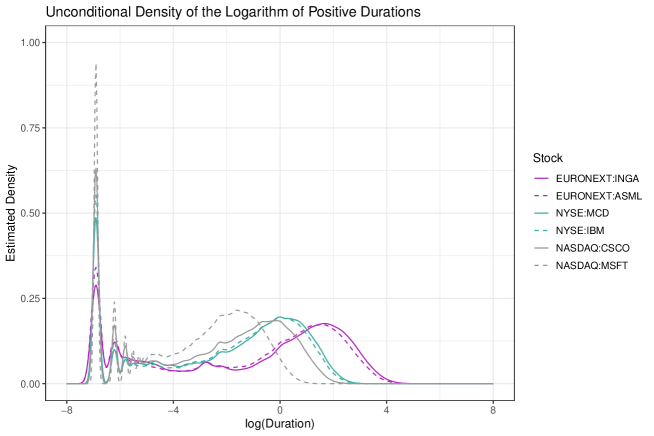
Figure 1: Density function of logarithmic durations estimated using the Gaussian kernel in June, 2021. Zero durations are excluded.

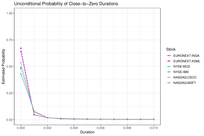
Figure 2: Probability of durations between 0 and 0.01 seconds in June, 2021.

2 Zero-Inflated ACD Model

Let $T_{0}\leq T_{1}\leq\cdots\leq T_{n}$ be random variables denoting times of transactions. Trade durations are then defined as $X_{i}=T_{i}-T_{i-1}$ for $i=1,\ldots,n$. As we operate in a discrete framework, we assume $T_{i}\in\mathbb{N}_{0}$, $i=0,\ldots,n$ and $X_{i}\in\mathbb{N}_{0}$, $i=1,\ldots,n$. We further assume trade durations $X_{i}$ to follow some given discrete distribution with conditional probability mass function $P[X_{i}=x_{i}|\theta]$, where $x_{i}$ are observations and $\theta=(\theta_{1},\ldots,\theta_{l})^{\prime}$ are parameters. First, we consider trade durations to follow the negative binomial distribution. Next, we extend the negative binomial distribution to capture excessive zeros using the zero-inflated model. Finally, we let parameters be time-varying with the generalized autoregressive score dynamics.

2.1 Negative Binomial Distribution

Non-negative integer variables are commonly analyzed using count data models based on specific underlying distribution, most notably the Poisson distribution and the negative binomial distribution (see Cameron and Trivedi, 2013). A distinctive feature of the Poisson distribution is that its expected value is equal to its variance. This characteristic is too strict in many applications as count data often exhibit overdispersion, a higher variance than the expected value. A generalization of the Poisson distribution overcoming this limitation is the negative binomial distribution with one parameter determining its expected value and another parameter determining its excess dispersion.

The negative binomial (NB) distribution can be derived in many ways (see Boswell and Patil, 1970). We use the NB2 parameterization of Cameron and Trivedi (1986) derived from the Poisson-gamma mixture distribution. It is the most common parametrization used in the negative binomial regression according to Cameron and Trivedi (2013). The probability mass function with scale parameter $\mu>0$ and dispersion parameter $\alpha\geq 0$ is

$$\mathrm{P}[X_{i}=x_{i}|\mu,\alpha]=\frac{\Gamma(x_{i}+\alpha^{-1})}{\Gamma(x_{i}+1)\Gamma(\alpha^{-1})}\left(\frac{\alpha^{-1}}{\alpha^{-1}+\mu}\right)^{\alpha^{-1}}\left(\frac{\mu}{\alpha^{-1}+\mu}\right)^{x_{i}}\quad\text{for }x_{i}=0,1,2,\ldots.$$ (1)

The expected value and variance is

$$\mathrm{E}[X_{i}] =\mu,$$ (2)

$$\mathrm{var}[X_{i}] =\mu(1+\alpha\mu).$$

Special cases of the negative binomial distribution include the Poisson distribution for $\alpha=0$ and the geometric distribution for $\alpha=1$.

2.2 Zero-Inflated Distribution

The zero-inflated distribution is an extension of a discrete distribution allowing the probability of zero values to be higher than the probability given by the original distribution. In the zero-inflated distribution, values are generated by two components – one component generates only zero values while the other component generates integer values (including zero values) according to the original distribution. Lambert (1992) proposed the zero-inflated Poisson model and Greene (1994) used zero-inflated model for the negative binomial distribution.

The zero-inflated negative binomial distribution is a discrete distribution with three parameters: scale parameter $\mu>0$, dispersion parameter $\alpha\geq 0$ and probability of excessive zero values $\pi\in[0,1)$. The variable $X_{i}$ follows the zero-inflated negative binomial distribution if

$$\begin{array}[]{ll}X_{i}\sim 0&\text{ with probability }\pi,\\ X_{i}\sim\mathrm{NB}(\mu,\alpha)&\text{ with probability }1-\pi.\\ \end{array}$$ (3)

The first process generates only zeros and corresponds to split transactions, while the second process generates values from the negative binomial distribution and corresponds to regular transactions. The probability mass function is

$$\mathrm{P}[X_{i}=0|\mu,\alpha,\pi] =\pi+(1-\pi)\left(\frac{\alpha^{-1}}{\alpha^{-1}+\mu}\right)^{\alpha^{-1}},$$ (4)

$$\mathrm{P}[X_{i}=x_{i}|\mu,\alpha,\pi] =(1-\pi)\frac{\Gamma(x_{i}+\alpha^{-1})}{\Gamma(x_{i}+1)\Gamma(\alpha^{-1})}\left(\frac{\alpha^{-1}}{\alpha^{-1}+\mu}\right)^{\alpha^{-1}}\left(\frac{\mu}{\alpha^{-1}+\mu}\right)^{x_{i}}\quad\text{for }x_{i}=1,2,\ldots.$$

The expected value and variance is

$$\mathrm{E}[X_{i}] =\mu(1-\pi),$$ (5)

$$\mathrm{var}[X_{i}] =\mu(1-\pi)(1+\pi\mu+\alpha\mu).$$

The score vector is given by

$$\nabla(x_{i},\mu,\alpha,\pi)=\begin{pmatrix}(\pi-1)(\alpha\mu+1)^{-1}\Big{(}1+\pi(\alpha\mu+1)^{\alpha^{-1}}-\pi\Big{)}^{-1}\\ \alpha^{-2}\Big{(}\ln(\alpha\mu+1)-\alpha\mu(\alpha\mu+1)^{-1}\Big{)}\Big{(}1-\pi(\pi-1)^{-1}(\alpha\mu+1)^{\alpha^{-1}}\Big{)}^{-1}\\ \Big{(}(\alpha\mu+1)^{\alpha^{-1}}-1\Big{)}\Big{(}1+\pi(\alpha\mu+1)^{\alpha^{-1}}-\pi\Big{)}^{-1}\\ \end{pmatrix}$$ (6)

for $x_{i}=0$ and

$$\nabla(x_{i},\mu,\alpha,\pi)=\begin{pmatrix}\mu^{-1}(x_{i}-\mu)(\alpha\mu+1)^{-1}\\ \alpha^{-2}\Big{(}\ln(\alpha\mu+1)+\alpha(x_{i}-\mu)(\alpha\mu+1)^{-1}+\psi_{0}(\alpha^{-1})-\psi_{0}(x_{i}+\alpha^{-1})\Big{)}\\ (\pi-1)^{-1}\\ \end{pmatrix}$$ (7)

for $x_{i}=1,2,\ldots$.

2.3 Generalized Autoregressive Score Dynamics

Generalized autoregressive score (GAS) models (Creal et al., 2013), also known as dynamic conditional score models (Harvey, 2013), capture dynamics of time-varying parameters $\tilde{f}_{i}=(\tilde{f}_{i,1},\ldots,\tilde{f}_{i,k})^{\prime}$ by the autoregressive term and the scaled score of the conditional observation density (or the conditional observation probability mass function in the case of discrete distribution). The time-varying parameters $\tilde{f}_{i}$ follow the recursion

$$\tilde{f}_{i+1}=C+B\tilde{f}_{i}+AS(\tilde{f}_{i})\nabla(x_{i},\tilde{f}_{i}),$$ (8)

where $C=(c_{1},\ldots,c_{k})^{\prime}$ are the constant parameters, $B=\mathrm{diag}(b_{1},\ldots,b_{k})$ are the autoregressive parameters, $A=\mathrm{diag}(a_{1},\ldots,a_{k})$ are the score parameters, $S(\tilde{f}_{i})$ is the scaling function for the score and $\nabla(x_{i},\tilde{f}_{i})$ is the score. In the original paper of Creal et al. (2013), authors noted that via the choice of the scaling function $S(\tilde{f}_{i})$, the GAS model allows for additional flexibility in how the score is used for updating $\tilde{f}_{i}$. The commonly used scaling functions in the GAS literature are based on the Fisher information matrix. We explored this option, however, we have not found it very suitable for the GAS model with the negative binomial distribution since the Fisher information for the parameter $\alpha$ does not have a closed-form. Consequently, the approximation of the Fisher information brings undue computational complexity resulting in an overly time-consuming optimization procedure. In order to keep our model simple, from now on we avoid the scaling, which is also a widely used option in the GAS literature. Moreover, Holý (2020) showed that the differences of models performance based on different scaling functions are negligible.

The long-term mean and unconditional value of the time-varying parameters is $\tilde{f}=(I-B)^{-1}C$. The parameters $\tilde{f}_{i}$ in (8) are assumed to be unbounded. However, some distributions require bounded parameters (e.g. variance greater than zero). The standard solution in the GAS framework is to use an unbounded parametrization $f_{i}=H(\tilde{f}_{i})$, which follows the GAS recursion instead of the original parametrization $\tilde{f}_{i}$, i.e.

$$f_{i+1}=c+bf_{i}+as(x_{i},f_{i}),$$ (9)

where $c$ are the constant parameters, $b$ are the autoregressive parameters, $a$ are the score parameters, and $s(x_{i},f_{i})$ is the reparametrized score. The reparametrized score equals to

$$s(x_{i},f_{i})=\dot{H}^{-1}(\tilde{f}_{i})\nabla(x_{i},\tilde{f}_{i}),$$ (10)

where $\dot{H}(\tilde{f}_{i})=\partial H(\tilde{f}_{i})/\partial\tilde{f}_{i}^{\prime}$ is the derivation of $H(\tilde{f}_{i})$.

The GAS specification includes many commonly used econometric models. For example, the GAS model with the normal distribution, the inverse of the Fisher information scaling and time-varying variance results in the GARCH model while the GAS model with the exponential distribution, the inverse of the Fisher information scaling and time-varying expected value results in the ACD model (Creal et al., 2013). The GAS framework can be utilized for discrete models as well. Koopman et al. (2018) used discrete copulas based on the Skellam distribution for high-frequency stock price changes. Koopman and Lit (2019) used the bivariate Poisson distribution for a number of goals in football matches and the Skellam distribution for a score difference. Gorgi (2018) used the Poisson distribution as well as the negative binomial distribution for offensive conduct reports. Holý and Tomanová (2021) used a mixture of double Poisson distributions to model price clustering in high-frequency prices.

2.4 Zero-Inflated Autoregressive Conditional Duration Model

We consider a model where observations follow the zero-inflated negative binomial distribution with the time-varying scale parameter $\mu_{i}$, time-varying dispersion parameter $\alpha_{i}$ and time-varying inflation parameter $\pi_{i}$ specified in (4). We use an unbounded parametrization with the exponential link for the scale and dispersion parameters and logistic transformation for the inflation parameter, i.e. $f_{i}=(\ln(\mu_{i}),\ln(\alpha_{i}),\ln(\pi_{i}/(1-\pi_{i})))^{\prime}$. Parameters $f_{i}$ are assumed to follow the recursion in (9), where the score for the zero-inflated negative binomial distribution is given by

$$s(x_{i},f_{i})=\begin{pmatrix}\mu_{i}(\pi_{i}-1)(\alpha_{i}\mu_{i}+1)^{-1}\Big{(}1+\pi_{i}(\alpha_{i}\mu_{i}+1)^{\alpha_{i}^{-1}}-\pi_{i}\Big{)}^{-1}\\ \alpha_{i}^{-1}\Big{(}\ln(\alpha_{i}\mu_{i}+1)-\alpha_{i}\mu_{i}(\alpha_{i}\mu_{i}+1)^{-1}\Big{)}\Big{(}1-\pi_{i}(\pi_{i}-1)^{-1}(\alpha_{i}\mu_{i}+1)^{\alpha_{i}^{-1}}\Big{)}^{-1}\\ \pi_{i}(1-\pi_{i})\Big{(}(\alpha_{i}\mu_{i}+1)^{\alpha_{i}^{-1}}-1\Big{)}\Big{(}1+\pi_{i}(\alpha_{i}\mu_{i}+1)^{\alpha_{i}^{-1}}-\pi_{i}\Big{)}^{-1}\\ \end{pmatrix}$$ (11)

for $x_{i}=0$ and

$$s(x_{i},f_{i})=\begin{pmatrix}(x_{i}-\mu_{i})(\alpha_{i}\mu_{i}+1)^{-1}\\ \alpha_{i}^{-1}\Big{(}\ln(\alpha_{i}\mu_{i}+1)+\alpha_{i}(x_{i}-\mu_{i})(\alpha_{i}\mu_{i}+1)^{-1}+\psi_{0}(\alpha_{i}^{-1})-\psi_{0}(x_{i}+\alpha_{i}^{-1})\Big{)}\\ -\pi_{i}\\ \end{pmatrix}$$ (12)

for $x_{i}=1,2,\ldots$.

3 Estimation and Asymptotic Properties

In this section, we focus on the model with the time-varying scale parameter $\mu_{i}$ and static dispersion $\alpha$ and inflation $\pi$ parameters. As such we set $f_{i}=\ln(\mu_{i})$ and $\theta=(\alpha,\pi,c,b,a)^{\prime}$. The score in (11) and (12) simplifies to

$$s(0,f_{i}) =\frac{(\pi-1)\exp(f_{i})}{(\alpha\exp(f_{i})+1)\left(1+\pi(\alpha\exp(f_{i})+1)^{\alpha^{-1}}-\pi\right)},$$ (13)

$$s(x_{i},f_{i}) =\frac{x_{i}-\exp(f_{i})}{\alpha\exp(f_{i})+1}\quad\text{for }x_{i}=1,2,\ldots.$$

For this GAS model with dynamics defined in (9) and (13), we establish the invertibility of the score filter and verify that sufficient conditions hold for the consistency and asymptotic normality of the maximum likelihood of the model parameters.

The static parameter vector $\theta$ is estimated by the method of maximum likelihood

$$\hat{\theta}_{n}\in\arg\max_{\theta\in\Theta}\hat{L}_{n}(\theta),$$ (14)

where $\hat{L}_{n}(\theta)$ denotes the log likelihood function obtained from a sequence of $n$ observations $x_{1},\ldots,x_{n}$, which depends on the filtered time-varying parameter $\hat{f}_{1}(\theta),...,\hat{f}_{n}(\theta)$. Since we are dealing with observation-driven filters which require an initialization value $\hat{f}_{1}$, we make an important distinction here between $\hat{L}_{n}(\theta)$ and $L_{n}(\theta)$. The first log likelihood is a function of the filtered parameter $\hat{f}_{1}(\theta),...,\hat{f}_{n}(\theta)$ initialized at a given value $\hat{f}_{1}$. The second likelihood is a function of the filtered parameter $f_{1}(\theta),...,f_{n}(\theta)$ initialized at the true unobserved value $f_{1}$. Of course, since $f_{1}$ is unobserved, we typically have that $\hat{f}_{1}\neq f_{1}$. In practice, the sample log likelihood is thus given by

$$\hat{L}_{n}(\theta)=\frac{1}{n}\sum_{i=1}^{n}\hat{\ell}_{i}(x_{i},\theta)=\frac{1}{n}\sum_{i=1}^{n}\ln\textrm{P}[X_{i}=x_{i}|\hat{f}_{i}(\theta),\theta].$$ (15)

In our case, the log likelihood is based on the zero-inflated negative binomial distribution

$$\ln\textrm{P}[X_{i}=0|\hat{f}_{i}(\theta),\theta] =\ln\left(\pi+(1-\pi)\left(\frac{\alpha^{-1}}{\alpha^{-1}+\mu_{i}}\right)^{\alpha^{-1}}\right),$$ (16)

$$\ln\textrm{P}[X_{i}=x_{i}|\hat{f}_{i}(\theta),\theta] =\ln(1-\pi)+\ln\frac{\Gamma(x_{i}+\alpha^{-1})}{\Gamma(x_{i}+1)\Gamma(\alpha^{-1})}+\frac{1}{\alpha}\ln\left(\frac{\alpha^{-1}}{\alpha^{-1}+\exp(\hat{f}_{i})}\right)$$

$$\quad+x_{i}\ln\left(\frac{\exp(\hat{f}_{i})}{\alpha^{-1}+\exp(\hat{f}_{i})}\right)\quad\text{for }x_{i}=1,2,\ldots.$$

Below, we show that the maximum likelihood estimator of the ZIACD model is consistent and asymptotically normal. The proof follows the structure laid down in Blasques et al. (2014), but we focus on the particular case of discrete data $\{x_{i}\}_{i\in\mathbb{N}}$ with a probability mass function $\textrm{P}[X_{i}=x_{i}|f_{i}(\theta),\theta]$. In contrast, Blasques et al. (2014) treat a general case for continuous data with a smooth probability density function.

3.1 Filter Invertibility

Filter invertibility is crucial for statistical inference in the context of observation-driven time-varying parameter models; see e.g. Straumann and Mikosch (2006), Wintenberger (2013), and Blasques et al. (2014). The filter $\{\hat{f}_{i}(\theta)\}_{i\in\mathbb{N}}$ initialized at some point $\hat{f}_{1}\in\mathbb{R}$ is said to be invertible if $\hat{f}_{i}(\theta)$ converges almost surely exponentially fast to a unique limit strictly stationary and ergodic sequence $\{f_{i}(\theta)\}_{i\in\mathbb{Z}}$,

$$|\hat{f}_{i}(\theta)-f_{i}(\theta)|\stackrel{{\scriptstyle eas}}{{\to}}0\quad\text{as}\quad i\to\infty.$$

Let $L_{n}(\theta)$ denote the log likelihood which depends on the limit time-varying parameter $f_{1}(\theta),...,f_{n}(\theta)$

$$L_{n}(\theta)=\frac{1}{n}\sum_{i=1}^{n}\ell_{i}(x_{i},\theta)=\frac{1}{n}\sum_{i=1}^{n}\ln\textrm{P}[X_{i}=x_{i}|f_{i}(\theta),\theta],$$

and let $L_{\infty}$ denote the limit log likelihood function

$$L_{\infty}(\theta)=\mathrm{E}[\ell_{i}(\theta)]=\mathrm{E}\left[\ln\textrm{P}[X_{i}=x_{i}|f_{i}(\theta),\theta]\right].$$

Proposition 1 appeals to the results in Blasques et al. (2014) to establish the invertibility of the score filter with zero-inflated negative binomial distribution as stated in (9) and (13). The proof presented in Technical Appendix A is an application of the results in Blasques et al. (2014) to our current model.

Proposition 1 (Filter invertibility).

Consider the score-driven model with zero-inflated negative binomial distribution in (9) and (13). Let the observed data $\{x_{i}\}_{i\in\mathbb{N}}$ be strictly stationary and ergodic, with a logarithmic moment $\mathrm{E}[\ln^{+}|x_{i}|]<\infty$, and let $\Theta$ be a compact parameter space defined as

$$\Theta=[\alpha^{-},\alpha^{+}]\cdot[\pi^{-},\pi^{+}]\cdot[c^{-},c^{+}]\cdot[b^{-},b^{+}]\cdot[a^{-},a^{+}]$$

and satisfying the following restrictions

$$\frac{a^{+}(\pi^{-}-1)^{2}}{2\alpha^{-}}+\frac{a^{+}|\pi^{-}-1|}{(\alpha^{-})^{2}}+b^{+} <1,$$

$$\mathrm{E}_{x_{i}>0}\left[\ln\left(\frac{a^{+}(\alpha^{+}x_{i}+1)}{4\alpha^{-}}+b^{+}\right)\right] <0.$$

Then the filter $\{\hat{f}_{i}(\theta)\}_{i\in\mathbb{N}}$ defined as $\hat{f}_{i+1}=c+b\hat{f}_{i}+as(x_{i},\hat{f}_{i})$ is invertible, uniformly in $\theta\in\Theta$.

3.2 Consistency

Proposition 1 gives us sufficient elements to characterize the asymptotic behavior of the ML estimator. This section uses existing theory on score models in Blasques et al. (2014) to verify the strong consistency of the ML estimator $\hat{\theta}_{n}$ as the sample size $n$ diverges to infinity.

For completeness, Lemma 1 states conditions for the consistency of the ML estimator. A sketch of the proof is offered in Technical Appendix A, and appropriate references are offered. This theorem naturally uses the invertibility properties established in Proposition 1 for our zero-inflated negative binomial score model. Following Blasques et al. (2014), this theorem allows for potential model mispecification.

Lemma 1 (Consistency of the ML estimator).

Let the conditions of Proposition 1 hold. Suppose further that the observed data has one bounded moment $\mathrm{E}[x_{i}]<\infty$, and let $\theta_{0}$ be the unique maximizer of the limit log likelihood function $\mathrm{E}[\ell_{i}(x_{i},\cdot)]:\Theta\to\mathbb{R}$ over the parameter space $\Theta$. Then $\hat{\theta}_{n}\stackrel{{\scriptstyle as}}{{\to}}\theta_{0}\in\Theta$ as $n\to\infty$.

3.3 Asymptotic Normality

Finally, we shed some light on the $\sqrt{n}$-consistency rate of $\hat{\theta}_{n}$ and the asymptotic normality of the standardized estimator $\sqrt{n}(\hat{\theta}_{n}-\theta_{0})$ as $n\to\infty$, when the model is well specified. For completeness, Lemma 2 summarizes standard conditions for asymptotic normality. A sketch of the proof is presented in Technical Appendix A, and we refer to Blasques et al. (2014) for additional details.

Lemma 2 (Asymptotic normality of the ML estimator).

Let the conditions of Lemma 1 hold. Suppose that the observed data has four bounded moments $\mathrm{E}|x_{i}|^{4}<\infty$, and let the true parameter lie in the interior of the parameter space, i.e. $\theta_{0}\in\mathrm{int}(\Theta)$. Finally, let the further regularity conditions stated in Theorem 4.16 of Blasques et al. (2014) hold. Then the ML estimator is asymptotically Gaussian

$$\sqrt{n}(\hat{\theta}_{n}-\theta_{0})\stackrel{{\scriptstyle d}}{{\to}}N(0,\mathcal{I}(\theta_{0})^{-1})\quad\text{as}\quad n\to\infty,$$

where $\mathcal{I}(\theta_{0})^{-1}$ denotes the inverse Fisher information matrix.

4 Empirical Study

4.1 Data Overview

In our empirical study, we analyze transaction data extracted from the Thomson Reuters Eikon. Eikon provides access to real-time market data and also contains historical intraday transactions. The data are taken from June to July of 2021. We analyze 6 stocks: ING Groep (INGA) and ASML Holding (ASML) which are listed on EURONEXT; McDonald’s Corporation (MCD) and International Business Machines Corporation (IBM) which are listed on NYSE; Cisco Systems, Inc. (CSCO) and Microsoft Corporation (MSFT) which are listed on NASDAQ.

We clean data using the following procedure. First, we delete observations with the timestamp outside the main trading hours and trading days. Second, for EURONEXT stocks, we delete all observations with the timestamps equal to the first timestamp of the day that occurs between 09:00:00 and 09:00:30. The reason is that the opening uncrossing (resulting from the morning auction) randomly occurs between 09:00:00 and 09:00:30. Third, we round the timestamp to the right precision (i.e. milliseconds) to fix the incorrect representation of the float.

The statistical characteristics for cleaned data are presented in Table 3. The two analyzed stocks listed on the NASDAQ belong to the most liquid stocks, while the stocks listed on the EURONEXT represent the least liquid stocks in our dataset. In June 2021, exact zero durations range from 43.01 percent (MCD) to 67.19 percent (ASML) and durations lower than 1 second form up to 98.57 percent (MSFT) of the dataset. For further descriptive statistics, see Table 3.

Table 3: Descriptive statistics of trade durations in June and July, 2021.

		EURONEXT		NYSE		NASDAQ
Statistic	Sample	INGA	ASML	MCD	IBM	CSCO	MSFT
% = 0	June	64.11	67.19	43.01	47.97	53.73	49.05
	July	57.78	65.66	46.01	48.75	54.14	48.93
% $<$ 0.01	June	73.70	76.30	56.98	61.63	66.86	63.86
	July	67.52	74.53	59.78	63.01	67.11	63.93
% $<$ 0.1	June	77.53	79.77	65.02	68.81	74.82	77.81
	July	71.86	78.50	67.18	71.13	74.48	79.20
% $<$ 1	June	82.31	84.73	82.91	85.72	91.37	98.57
	July	78.37	85.11	84.59	88.75	90.72	99.05
Mean	June	1.56	1.19	0.58	0.47	0.26	0.10
	July	1.72	0.91	0.52	0.37	0.29	0.08
Variance	June	27.85	18.69	1.90	1.43	0.54	0.05
	July	26.01	10.31	1.72	1.02	0.63	0.04
Std. Dev.	June	5.28	4.32	1.38	1.19	0.73	0.23
	July	5.10	3.21	1.31	1.01	0.79	0.20
95%-Quantile	June	9.94	7.50	3.25	2.70	1.60	0.54
	July	10.48	5.66	2.96	2.14	1.73	0.46
Obs. per Min.	June	38.48	50.50	103.55	128.53	227.47	622.69
	July	34.88	66.00	115.11	163.22	210.39	723.17

4.2 In-Sample Performance

We use the proposed ZIACD model based on the zero-inflated negative binomial distribution with the time-varying scale, dispersion, and zero inflation parameters to fit observed durations rounded down to hundredths of a second using data from June 2021. The estimated coefficients are reported in Table 4. All coefficients are significant at any reasonable level and their standard deviations are virtually zero due to huge sample sizes ranging from 431463 (INGA) to 5342667 (MSFT). We, therefore, report only the estimated values. The numbers of observations per minute are also reported in Table 3. As expected, the coefficient controlling the impact of the score $a$ is positive for all three parameters and all six stocks. This means that the score serves as a correction term that adjusts the time-varying parameters for the observed values. The autoregressive coefficient $b$ is also positive and quite high for all three parameters and all six stocks. In the case of the scale parameter, it is very close to one signaling high persistence of the time series.

Table 5 reports the average values of the scale, dispersion, and zero inflation parameters over time. Note that the average scale parameter (adjusted to seconds) is much higher than the sample mean reported in Table 3 as our model is able to separate zeros attributed to split transactions which subsequently do not affect the scale parameter. On average, between 53.27 percent (MCD) and 74.88 percent (ASML) of all durations are excessive zeros generated by split transactions depending on the stock. This corresponds to the ratio of excessive zeros to all zeros ranging between 91.81 percent (MSFT) and 98.13 percent (ASML). In other words, between 1.87 percent (ASML) and 8.19 percent (MSFT) of zero durations are generated by unrelated transactions which should not be discarded from the data.

Table 5 also evaluates the fit of the ZIACD model. The mean absolute error is between 0.11 seconds (MSFT) and 2.50 seconds (INGA) while the root mean square error is between 0.21 (MSFT) and 5.22 (INGA). These values are quite high when compared to the predicted value $\mu_{i}(1-\pi_{i})$, on which both errors are based, with its mean ranging from 0.09 seconds (MSFT) to 1.58 seconds (INGA). This is caused by the fact that the predicted value is not very representative of the whole distribution as, on average, between 53.27 percent (MCD) and 74.88 percent (ASML) of all values are exactly zero while the rest have expected value between 0.22 seconds (MSFT) and 5.68 seconds (INGA). It is therefore more suitable to assess the fit of the model based on the whole distribution.

We focus on the probability of zeros given by the model. Table 5 reports the mean probabilities of zero value given by the model when the observed value is indeed zero and when the observed value is positive. For the INGA and ASML stocks, the difference between these two probabilities is lower than one percent suggesting a limited benefit of the dynamics in the zero-inflation parameter. For the more traded stocks, the difference is between 5.78 percent (MCD) and 9.58 percent (CSCO) suggesting a certain degree of predictive ability of the zero-inflation dynamics.

Figure 3 studies the fit of the model in more detail by comparing the average conditional probabilities given by the ZIACD model with the unconditional empirical distribution. The largest deviation is -0.68 percent at 0.01 seconds for the MCD stock. This deviation is rather small but uncovers a systematic error as the probability of 0.01 durations is underestimated for all stocks. Similar underestimation is also present at 0.06 seconds for the ASML and INGA stocks traded on the EURONEXT exchange and at 0.10 seconds for all stocks. The latter two anomalies are also visible in Figure 1 at -2.81 and -2.30 log-durations. The proposed model is therefore incorrectly specified and the true distribution of durations is much more complex. Nevertheless, the deviations of the conditional ZIACD probabilities are quite small and the model is usable in practice.

Table 4: The estimated coefficients of the zero-inflated negative binomial model.

		EURONEXT		NYSE		NASDAQ
Parameter	Coef.	INGA	ASML	MCD	IBM	CSCO	MSFT
	$c$	0.006068	0.002591	0.000011	0.000151	0.000180	0.000064
Scale	$a$	0.109420	0.089377	0.032544	0.032434	0.051552	0.032155
	$b$	0.998958	0.999509	0.999996	0.999954	0.999913	0.999938
	$c$	0.006364	0.061190	0.148700	0.129161	0.042488	0.000869
Dispersion	$a$	0.057713	0.216293	0.289589	0.243921	0.136988	0.021367
	$b$	0.992826	0.927438	0.806245	0.815294	0.948153	0.998387
	$c$	0.030722	0.017910	0.048158	0.138758	0.116703	0.119207
Zero Inflation	$a$	0.164058	0.100389	2.129143	2.177550	2.672883	2.542853
	$b$	0.968110	0.983785	0.680476	0.668047	0.856934	0.743213

Table 5: The mean scale parameter (in seconds), the mean dispersion parameter, the mean inflation parameter (in percent), the mean ratio of zeros caused by split transactions (in percent), the mean predicted value (in seconds), the mean absolute error (in seconds), the root mean square absolute error (in seconds), the mean probabilities of zero value given by the zero-inflated negative binomial model when the observation is either zero or positive (in percent), and the mean log-likelihood.

	EURONEXT		NYSE		NASDAQ
Variable	INGA	ASML	MCD	IBM	CSCO	MSFT
Mean Scale	5.68	4.89	1.28	1.14	0.70	0.22
Mean Dispersion	2.45	2.35	2.17	2.02	2.26	1.70
Mean Zero Inflation	72.06	74.88	53.27	58.60	63.01	58.63
Mean Split Ratio	97.78	98.13	93.49	95.09	94.23	91.81
Mean Predicted Value	1.58	1.22	0.60	0.48	0.27	0.09
Mean Absolute Error	2.50	1.96	0.72	0.59	0.31	0.11
Root Mean Square Error	5.22	4.28	1.29	1.11	0.66	0.21
$\mathrm{P}[X_{i}=0]$ When $x_{i}=0$	67.48	67.97	65.60	66.47	69.15	69.66
$\mathrm{P}[X_{i}=0]$ When $x_{i}>0$	67.09	67.74	59.81	60.62	59.57	61.52
Mean Log-Likelihood	-2.42	-2.17	-3.01	-2.69	-2.16	-2.00

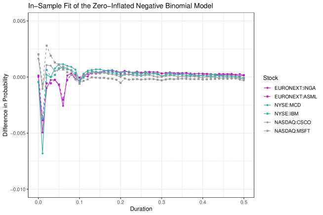
Figure 3: The in-sample difference between the conditional probabilities given by the zero-inflated negative binomial model and the unconditional distribution of observations.

4.3 Out-of-Sample Performance

In this section, we use the models estimated using durations from June 2021 and perform one-step-ahead forecasts during July 2021 to assess their long-term behavior. Figure 4 shows deviations of the average out-of-sample conditional probabilities given by the ZIACD model from the unconditional empirical distribution. Similarly to Figure 3, the probabilities at 0.01, 0.06, and 0.10 seconds are systematically underestimated. However, the highest deviations are in the case of the probabilities of zero durations. The difference in probability reaches 3.02 percent (INGA) and drops down to -1.25 percent (MCD). This is related to a change in the occurrence of zero values in July. According to Table 3, the unconditional probability of zero values decreases from 64.11 to 57.78 percent for the INGA stock while it increases from 43.01 to 46.01 percent for the MCD stock. Note that the other descriptive statistics in Table 3 also change considerably.

Our model has therefore a limited predictive ability in the long term and should be used only for short-term predictions. To capture changing characteristics of durations, a non-stationary model could be used. In the context of financial duration modeling, non-stationary ACD models were studied by Bortoluzzo et al. (2010) and Mishra and Ramanathan (2017). We leave an analysis of long-term dynamics of excessive zero probability as a topic for future research.

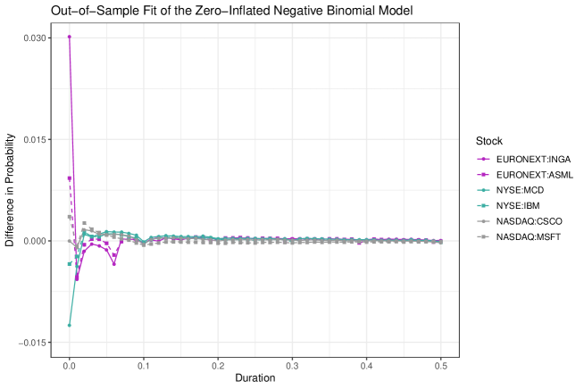
Figure 4: The out-of-sample difference between the conditional probabilities given by the zero-inflated negative binomial model and the unconditional distribution of observations.

4.4 Model Specification

We compare the proposed ZIACD model, which is based on the zero-inflated negative binomial distribution and has all three parameters time-varying, with models imposing some restrictions. Specifically, Table 7 compares models based on the Poisson, geometric, and negative binomial distributions together with their zero-inflated versions. All parameters in these models are time-varying. On the other hand, Table 6 compares models based on the zero-inflated negative binomial distribution with some parameters static and some time-varying. We use two criteria to compare the models – the difference in the Akaike information criterion (AIC) for the in-sample fit and the Diebold-Mariano (DM) statistic for the out-of-sample fit. When comparing two models, a positive difference in the AIC favors the second model over the first model while a positive value of the DM statistic favors the first model over the second model. The DM statistic has asymptotically the standard normal distribution under the null hypothesis of equivalent out-of-sample log-likelihoods. More details on these criteria are given in Technical Appendix B. Not surprisingly in such large datasets, the most general specification of the model has the best fit. We do not report $p$-values for the DM statistic as it is significant at any reasonable level in all cases due to huge sample sizes.

There is clear evidence of overdispersion, i.e. the variance higher than the expected value. According to Table 5, the average value of the dispersion parameter $\alpha$ in the zero-inflated negative binomial model ranges between $1.70$ (MSFT) and $2.45$ (INGA). This favors the negative binomial distribution over the Poisson distribution with fixed $\alpha=0$ and the geometric distribution with fixed $\alpha=1$. Overdispersion is also supported by the difference in the AIC and the DM statistic reported in Table 6. The Poisson distribution has the highest AIC for all stocks while the geometric distribution has the worst DM statistic compared to the zero-inflated negative binomial distribution. One possible reason for overdispersion could just be the presence of excessive zeros. Indeed, the zero-inflated Poisson and geometric distributions perform better than their original versions. However, they are still inferior to the zero-inflated negative binomial distribution suggesting that there is overdispersion present in non-zero values as well. Table 7 further shows that the specification with the time-varying dispersion parameter performs significantly better than the static one. This improvement of the in-sample and out-of-sample fit is, however, the smallest among all specifications in Tables 6 and 7. For some smaller data samples of less traded assets or with shorter periods of time (such as a day), the model with static dispersion parameter might be more suitable due to possible overfitting.

Our analysis also reveals the presence of excessive zeros suggesting the existence of the process generating only zero values (i.e. split transactions) alongside the process generating regular durations. According to Table 5, the average probability of excessive zeros $\pi$ in the zero-inflated negative binomial model ranges between 53.27 percent (MCD) and 74.88 percent (ASML). The presence of excessive zeros is further supported by the better in-sample and out-of-sample fit for the zero-inflated distributions as reported in Table 6. Table 7 shows that it is also suitable to let the zero-inflation parameter be time-varying as this increases the in-sample and out-of-sample fit, particularly for the more traded stocks MCD, IBM, CSCO, and MSFT. This is in line with the mean probabilities of zero value when the observation is either zero or positive reported in Table 5.

Table 6: The difference in the Akaike information criterion (AIC) and the Diebold–Mariano (DM) statistic for the models based on the Poisson distribution (P), the geometric distribution (G), the negative binomial distribution (NB), the zero-inflated Poisson distribution (ZIP), the zero-inflated geometric distribution (ZIG), and the zero-inflated negative binomial distribution (ZINB).

		EURONEXT		NYSE		NASDAQ
Distribution	Crit.	INGA	ASML	MCD	IBM	CSCO	MSFT
P / ZINB	AIC	267461915.62	280418352.77	138404692.48	148394239.86	142150126.37	124884854.32
	DM	-235.37	-269.95	-384.02	-436.68	-361.32	-945.72
G / ZINB	AIC	2995721.03	3894926.03	3283604.41	4270769.74	6100642.18	10641774.31
	DM	-689.62	-981.64	-793.38	-953.95	-668.61	-1272.63
NB / ZINB	AIC	45891.96	58214.58	118521.51	153740.09	279306.75	617624.25
	DM	119.12	-138.71	-221.39	-261.55	-287.93	-469.99
ZIP / ZINB	AIC	182851270.41	100937602.51	60299913.57	58956197.68	58305592.35	43332973.41
	DM	-134.68	-207.14	-291.16	-311.60	-336.45	-617.43
ZIG / ZINB	AIC	49991.79	50910.51	84210.77	77231.38	122581.75	112468.26
	DM	-80.79	-97.10	-108.19	-113.01	-123.58	-144.40

Table 7: The difference in the Akaike information criterion (AIC) and the Diebold–Mariano (DM) statistic for the zero-inflated negative binomial model with all parameters static (SSS), dynamic $\mu$ (DSS), dynamic $\mu$, $\alpha$ (DDS), dynamic $\mu$, $\pi$ (DSD), and dynamic $\mu$, $\alpha$, $\pi$ (DDD).

		EURONEXT		NYSE		NASDAQ
Dynamics	Crit.	INGA	ASML	MCD	IBM	CSCO	MSFT
SSS / DDD	AIC	21492.36	27667.68	264677.50	325382.37	839689.51	1780799.16
	DM	-86.74	-133.22	-302.72	-393.75	-425.24	-762.36
DSS / DDD	AIC	8135.80	7612.61	219595.15	271386.43	742989.86	1447522.61
	DM	-57.16	-71.11	-274.29	-321.08	-396.20	-619.05
DDS / DDD	AIC	5652.62	4831.46	86375.83	112311.74	212495.87	521863.12
	DM	-50.55	-56.63	-177.80	-208.29	-231.05	-420.17
DSD / DDD	AIC	1617.11	1953.18	7286.14	5069.21	6614.27	9203.83
	DM	-13.99	-24.88	-32.19	-35.19	-24.04	-32.57

4.5 Degree of Rounding

The choice of rounding to hundredths of a second, i.e. centiseconds, is motivated by Figure 2 which shows that the majority of excessive close-to-zero durations is concentrated in values 0 and 0.001 and the occurrence of larger values quickly decreases. In this section, we study the impact of different degrees of rounding and whether this choice is appropriate. Again, we use the difference in the AIC to assess the in-sample fit and the DM statistic to assess the out-of-sample fit. When comparing two models with different degrees of rounding, we compute the log-likelihood (which is the base for both AIC and DM) with respect to the rounding to fewer decimal places. A probability under the rounding to fewer decimal places is then the sum of the corresponding probabilities under the rounding to more decimal places. We consider rounding to zero decimal places (seconds), one decimal place (deciseconds), two decimal places (centiseconds), and three decimal places (milliseconds), i.e. the original data.

Table 8 shows the impact of increasing rounding. The rounding to centiseconds is clearly preferred over no rounding, i.e. precision to milliseconds. This is caused by the inability of the ZIACD model on milliseconds to account for an excessive probability of durations between 0.001 and 0.009 seconds; mostly, however, 0.001 seconds. The choice between the rounding to centiseconds and deciseconds differs for the individual stocks. For the INGA and AMSL stocks traded on the EURONEXT exchange, the model on deciseconds performs better. The difference in the AIC and the value of the DM statistic suggesting deciseconds are significant but smaller compared to the other values in Table 8. To keep the reported results simple, we stick with the model on centiseconds. For the more trade stocks MCD, IBM, CSCO, and MSFT, the model on centiseconds clearly outperforms the model on deciseconds. Finally, deciseconds are preferred over seconds for all stocks.

Table 8: The difference in the Akaike information criterion (AIC) and the Diebold–Mariano (DM) statistic for the zero-inflated negative binomial model based on data rounded to milliseconds (ms), centiseconds (cs), deciseconds (ds), and seconds (s).

		EURONEXT		NYSE		NASDAQ
Precision	Crit.	INGA	ASML	MCD	IBM	CSCO	MSFT
ms / cs	AIC	28004.18	37387.09	49082.84	58915.61	42215.74	178862.15
	DM	-74.72	-102.18	-101.74	-97.79	-32.09	-114.94
cs / ds	AIC	3085.80	4326.46	-18588.85	-28803.35	-66676.58	-233114.94
	DM	-11.59	-29.46	47.73	76.70	87.26	218.61
ds / s	AIC	-1071.15	-1021.23	-34331.20	-42690.00	-70647.10	-34682.20
	DM	10.75	12.33	87.23	97.62	105.13	65.45

4.6 Comparison to Continuous Models

We compare the proposed discrete ZIACD model with continuous models based on the generalized gamma distribution (see Technical Appendix C) with GAS dynamics. The generalized gamma distribution contains the exponential, Weibull, and gamma distributions as special cases and belongs to the family of the generalized F distribution. The use of the generalized gamma distribution in ACD models was proposed by Lunde (1999). Both Bauwens et al. (2004) and Fernandes and Grammig (2005) found that the generalized gamma distribution is more adequate than the exponential, Weibull, and Burr distributions. The study Xu (2013) shows that the log-normal distribution does not outperform the generalized gamma distribution either. For these reasons, the generalized gamma distribution is our main candidate for the competing continuous distribution. In our comparison, we do not consider the generalized F distribution as it has four parameters and in most cases of financial durations reduces to the generalized gamma distribution as discussed by Hautsch (2003) and Hautsch (2012). We also do not consider the Birnbaum–Saunders distribution as it models the median instead of the scale parameter and therefore does not strictly belong to the traditional ACD class. Models based on continuous distributions must address the issue of zero durations. We consider two ways of dealing with zero values in continuous models – discarding them and truncating them to a given value. Furthermore, we consider three values for truncating – 0.001, 0.0005, and 0.0001 seconds. Bauwens (2006) used truncation to the half of the smallest increment, which is 0.0005 seconds in our case. Similarly to the previous section, we compute log-likelihood on a discrete grid of centiseconds. In the case of discarding zeros, we compare the generalized gamma model with the zero-inflated negative binomial model that is also estimated without zero values.

Figures 5 and 6 demonstrate the unsuitability of the approach discarding zeros. Similarly to figures 3 and 4, the generalized gamma model is not able to capture unusually increased occurrence of 0.06 seconds (for the INGA and ASML stocks) and 0.10 seconds (for all stocks). A crucial problem, however, is significantly underestimated probabilities in the wider vicinity of zero. In the case of the zero value itself, the difference in probability reaches -10.17 percent for the AMSL stock. Note that figures 5 and 6 have much larger scale than figures 3 and 4. Table 9 then confirms the superiority of the ZIACD model over the continuous alternatives in terms of the difference in the AIC and the DM statistic. Concerning the treatment of zero values, we can see that it is better to truncate zeros to smaller values but it is even better to just discard them. Either way, the results imply that the loss of decimal places in the proposed ZIACD model is of much less importance than the incorrect treatment of zero values in the continuous models.

Table 9: The difference in the Akaike information criterion (AIC) and the Diebold–Mariano (DM) statistic for the generalized gamma model (GG) with zeros discarded (Discard) or truncated (Trunc) and the zero-inflated negative binomial model (ZINB).

		EURONEXT		NYSE		NASDAQ
Model	Crit.	INGA	ASML	MCD	IBM	CSCO	MSFT
GG Discard / ZINB Discard	AIC	14808.54	18250.42	24298.96	32947.27	69568.44	143388.68
	DM	-41.41	-48.97	-72.66	-81.80	-103.98	-143.54
GG Trunc to 0.001 / ZINB	AIC	268465.60	356579.92	360491.17	469852.80	671361.23	1361317.34
	DM	-293.92	-386.13	-343.09	-387.75	-363.67	-548.30
GG Trunc to 0.0005 / ZINB	AIC	218184.60	302587.55	325384.37	406923.28	565376.30	1219524.80
	DM	-245.36	-337.90	-203.66	-342.98	-222.98	-524.67
GG Trunc to 0.0001 / ZINB	AIC	167265.34	225896.55	282777.70	329205.71	426886.17	1000254.88
	DM	-196.87	-271.27	-261.23	-299.34	-246.49	-449.19

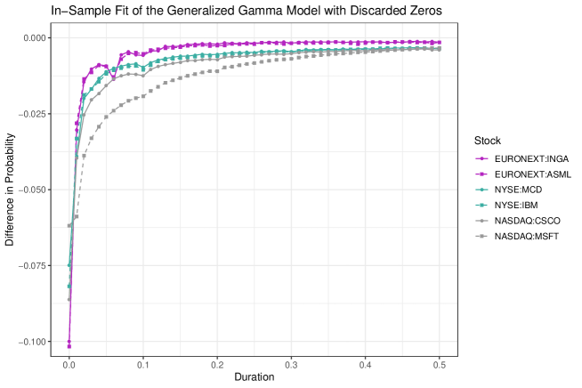
Figure 5: The in-sample difference between the conditional probabilities given by the generalized gamma model with discarded zeros and the unconditional distribution of observations.

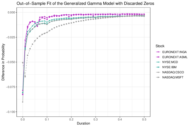
Figure 6: The out-of-sample difference between the conditional probabilities given by the generalized gamma model with discarded zeros and the unconditional distribution of observations.

5 Discussion

5.1 Discreteness of Data

As mentioned above, our paper studies data with high-precision timestamps. Although it is nowadays quite common that exchanges record transactions with precision to one millisecond or higher, one can encounter preprocessed datasets with precision to one second due to their easier readability. In some cases, this can even be the only dataset provided by the exchange to the public. For these low-precision data, it is more natural to use a discrete model such as ours rather than a continuous model.

To our knowledge, Grimshaw et al. (2005) is the only paper addressing the issue of rounding in financial durations analysis. They found that ignoring the discreteness of data leads to a distortion of time-dependence tests in financial durations. More loosely related, Schneeweiss et al. (2010) reviewed the bias-inducing effects of rounding. Tricker (1984) and Taraldsen (2011) explored the effects of rounding on the exponential distribution while Tricker (1992) dealt with the gamma distribution. Zhang et al. (2010) and Li and Bai (2011) found that the rounding errors in autoregressive processes can further accumulate making continuous models unreliable.

Let us conduct the following experiment to explore the influence of rounding on the estimation of GAS models based on discrete and continuous distributions. We simulate 10000 observations using a dynamic model based on the generalized gamma distribution with the time-varying scale parameter following the GAS dynamics given by $c=0.10$, $a=0.10$, $b=0.90$ and the two static shape parameters $\theta=0.50$ and $\varphi=0.50$. The unconditional mean is then approximately equal to 2.05. Then, we round down the observations to a given number of decimal places. Finally, using rounded observations, we estimate GAS models based on the generalized gamma distribution with zero values (created by the rounding) either discarded or truncated as well as the GAS model based on the negative binomial distribution. Note that we do not consider zero inflation in the negative binomial distribution as there are no excessive zeros generated by a different process. The simulation is repeated 1000 times. Figure 7 shows the bias of the unconditional mean of the estimated models with data rounded down to decimal places ranging from 3 up to 6. The negative binomial model, although with incorrectly specified distribution, has the smallest bias. On the other hand, the generalized gamma model with either treatment of zero values has a much higher bias which increases with rounding to fewer decimal places. This is caused by an increased occurrence of discarded or truncated zero values which significantly distorts the continuous distribution. This experiment demonstrates that it is more appropriate to use a distribution that is able to handle zero values, even though it is not the true distribution of the data generating process.

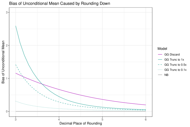
Figure 7: The bias of the unconditional mean given by the generalized gamma model (GG) with zeros discarded (Discard) or truncated (Trunc) and the negative binomial model (NB).

5.2 Other Mixture Models

On a final note, we discuss some potential alternatives to our proposed model that also utilize a mixture of two processes to capture unrelated and split transactions.

One possibility is to consider a hurdle model based on a continuous distribution with a point mass at zero. For example, the dynamic zero-augmented model of Hautsch et al. (2014) or the dynamic censoring model of Harvey and Ito (2020) could be used. Hautsch et al. (2014) proposed a multiplicative error model based on a zero-augmented distribution and applied it to high-frequency time series of cumulated trading volumes. Harvey and Ito (2020) proposed a dynamic model with a left-shifted distribution for non-zero observations and censored negative values and applied it to daily rainfalls in northern Australia. Note that similarly to us, Harvey and Ito (2020) utilized the GAS framework. There are, however, two issues with this approach. Without any transformation of data, both these models would require split transactions to result in exactly zero durations, which is not realistic as shown in Section 1. Of course, one could follow our approach and round down durations below a given threshold, e.g. one hundredth of a second, to zero. Unlike in our approach, only durations below the threshold would be rounded and durations above would be kept continuous. The second issue is that hurdle models assume that one process generates zero values while the other process generates positive values only. In other words, it would not be possible to determine the ratio between zeros caused by unrelated and split transactions as all zeros would be attributed solely to split transactions. For this reason, our proposed model is superior.

A more complex approach is to assume a non-trivial process for split transactions. Both processes would then generate positive values and at least one of them would also generate zero values. This could be accomplished within either a continuous or discrete framework depending on the underlying data. The choice of a continuous distribution for the process governing split transactions would, however, be limited as zero is required to lie in its support. An exponential distribution would be an obvious starting point here. Note that the appropriately chosen process governing split transactions would not require any transformation of data, which would be a major benefit. On the other hand, the potential complexity of such a model could be a drawback. The ACD model based on a mixture of two non-trivial processes is the direction of our future research.

6 Conclusion

We analyze trade durations with split transactions manifesting themselves as zero and close-to-zero values. We round down durations to hundredths of a second and approach this problem within a discrete framework. To capture excessive zero values and autocorrelation structure in durations, we propose a model based on the zero-inflated negative binomial distribution with score dynamics for the time-varying parameters. We label this model the zero-inflated autoregressive conditional duration model or ZIACD model for short. The paper has three main contributions.

1. We extend the theory of GAS models for the zero-inflated negative binomial distribution with time-varying scale parameter. Specifically, we establish the invertibility of the score filter. We also derive sufficient conditions for the consistency and asymptotic normality of the maximum likelihood of the model parameters.

2. We argue that zero durations should not be removed from the data as they can correspond not only to split transactions but to unrelated transactions as well. Even more, split transactions can generate not only zero values but positive values as well. In the empirical study, the proposed model identifies that split transactions form between 92 and 98 percent of durations smaller than 0.01 seconds. Furthermore, between 53 and 75 percent of all durations correspond to split transactions.

3. We compare the proposed discrete approach with the commonly used continuous approach. We find that even when durations are recorded with high precision suitable for continuous modeling, the proposed discrete model estimated from rounded durations outperforms traditional continuous models based on unrounded data due to its correct treatment of zero and close-to-zero values.

Our proposed model can be utilized in joint modeling of prices and durations. It also allows studying the trading process from the market microstructure perspective. Future research should focus on more complex mixture models, whether in discrete or continuous frameworks, that do not require any transformation of data. However, it should be noted, that these complex models might lose the benefits of our ZIACD model such as simple implementability in practice and verifiability of sufficient conditions for asymptotic properties of the estimator.

Funding

The work of Francisco Blasques was supported by the Dutch Science Foundation (NWO) under project VI.Vidi.195.099. The work of Vladimír Holý was supported by the Internal Grant Agency of the University of Economics, Prague under project F4/21/2018. The work of Petra Tomanová was supported by the Czech Science Foundation under project 19-02773S.

Appendix A Proofs of Asymptotic Properties

Proof of Proposition 1:

Following Straumann and Mikosch (2006) and Blasques et al. (2014), we obtain invertibility by verifying that the conditions of Theorem 3.1 of Bougerol (1993) hold uniformly on a non-empty set $\Theta$, for any initialization $\hat{f}_{1}(\theta)$ In particular, we note that a $\ln^{+}$ bounded moment holds at $i=1$ since

$$\mathrm{E}\left[\log^{+}\sup_{\theta\in\Theta}\left|c+b\hat{f}_{1}(\theta)+as(x_{1},\hat{f}_{1}(\theta))\right|\right] \leq 4\ln 2+\mathrm{E}\left[\ln^{+}\sup_{\theta\in\Theta}|c|\right]+\mathrm{E}\left[\ln^{+}\sup_{\theta\in\Theta}\left|b\hat{f}_{1}(\theta)\right|\right]$$

$$\quad+\mathrm{E}\left[\ln^{+}\sup_{\theta\in\Theta}\left|as(x_{1},\hat{f}_{1}(\theta))\right|\right]$$

$$\leq 4\ln 2+\mathrm{E}\left[\ln^{+}\sup_{\theta\in\Theta}|c|\right]+\mathrm{E}\left[\ln^{+}\sup_{\theta\in\Theta}|b|\right]$$

$$\quad+\mathrm{E}\left[\ln^{+}\sup_{\theta\in\Theta}\left|\hat{f}_{1}(\theta)\right|\right]+\mathrm{E}\left[\ln^{+}\sup_{\theta\in\Theta}|a|\right]$$

$$\quad+\mathrm{E}\left[\sup_{\theta\in\Theta}\left|s(x_{1},\hat{f}_{1}(\theta))\right|\right]$$

$$\leq 4\ln 2+\max\{|c^{-}|,|c^{+}|\}+\max\{|b^{-}|,|b^{+}|\}$$

$$\quad+\sup_{\theta\in\Theta}\left|\hat{f}_{1}(\theta)\right|+\max\{|a^{-}|,|a^{+}|\}+\mathrm{E}\left[\ln^{+}\sup_{\theta\in\Theta}\left|s(x_{1},\hat{f}_{1}(\theta))\right|\right]$$

$$<\infty,$$

where the three inequalities follow by norm sub-additivity, as well as the $\ln^{+}$ sub-additive and sub-multiplicative inequalities in Lemma 2.2 of Straumann and Mikosch (2006), and the last bound follows since $c$, $b$, $a$ are strictly positive and lie on the compact $\Theta$ and $\hat{f}_{1}(\theta)$ is a given real number. We also have that $\mathrm{E}\left[\ln^{+}\sup_{\theta\in\Theta}|s(x_{1},\hat{f}_{1}(\theta))|\right]<\infty$ as

$$\mathrm{E}\left[\ln^{+}\sup_{\theta\in\Theta}\left|s(x_{i},\hat{f}_{1}(\theta),\theta)\right|\right] =\mathrm{P}[x_{i}=0]\cdot\ln^{+}\sup_{\theta\in\Theta}\left|s(0,\hat{f}_{1}(\theta),\theta)\right|$$

$$\quad+\mathrm{P}[x_{i}>0]\cdot\mathrm{E}_{x_{i}>0}\left[\ln^{+}\sup_{\theta\in\Theta}\left|s(x_{i},\hat{f}_{1}(\theta),\theta)\right|\right]$$

$$\leq\ \ln^{+}\sup_{\theta\in\Theta}\left|s(0,\hat{f}_{1}(\theta),\theta)\right|+\mathrm{E}_{x_{i}>0}\left[\ln^{+}\sup_{\theta\in\Theta}\left|s(x_{i},\hat{f}_{1}(\theta),\theta)\right|\right]$$

$$<\infty,$$

where $\mathrm{E}_{x_{i}>0}$ denotes the conditional expectation $\mathrm{E}_{x_{i}>0}[\cdot]=\mathrm{E}[\cdot|x_{i>0}]$ and

$$\mathrm{E}\left[\ln^{+}\sup_{\theta\in\Theta}|s(0,\hat{f}_{1},\theta)|\right] =\ln^{+}\sup_{\theta\in\Theta}|s(0,\hat{f}_{1},\theta)|$$

$$=\ln^{+}\sup_{\theta\in\Theta}\Big{|}(\pi-1)\exp(\hat{f}_{1})(\alpha\exp(\hat{f}_{1})+1)^{-1}$$

$$\qquad\cdot\left(1+\pi(\alpha\exp(\hat{f}_{1})+1)^{\alpha^{-1}}-\pi\right)^{-1}\Big{|}$$

$$\leq\ln^{+}\sup_{\theta\in\Theta}|\pi-1|+\ln^{+}\sup_{\theta\in\Theta}|\exp(\hat{f}_{1})|+\ln^{+}\sup_{\theta\in\Theta}|(\alpha\exp(\hat{f}_{1})+1)^{-1}|$$

$$\qquad+\ln^{+}\sup_{\theta\in\Theta}\Big{|}\Big{(}1+\pi(\alpha\exp(\hat{f}_{1})+1)^{\alpha^{-1}}-\pi\Big{)}^{-1}\Big{|}$$

$$<\infty,$$

which holds as the parameter vector $\theta$ lies on the compact set $\Theta$, and $\hat{f}_{1}$ is a given point in $\mathbb{R}$, and

$$\mathrm{E}_{x_{i}>0}\left[\ln^{+}\sup_{\theta\in\Theta}\left|s(x_{i},\hat{f}_{1},\theta)\right|\right] =\mathrm{E}_{x_{1}>0}\left[\ln^{+}\sup_{\theta\in\Theta}\left|x_{1}-\exp(\hat{f}_{1})(\alpha\exp(\hat{f}_{1})+1)^{-1}\right|\right]$$

$$\leq\mathrm{E}_{x_{1}>0}\left[\ln^{+}\sup_{\theta\in\Theta}\left|x_{1}-\exp(\hat{f}_{1})\right|\right]$$

$$\leq 2\ln(2)+\mathrm{E}_{x_{1}>0}\left[\ln^{+}|x_{1}|\right]+\ln^{+}|\exp(\hat{f}_{1})|$$

$$<\infty,$$

since $x_{1}$ has a logarithmic moment, $\Theta$ is compact and $\hat{f}_{1}\in\mathbb{R}$.

Finally, the contraction condition of Bougerol (1993) is satisfied uniformly in $\theta\in\Theta$ since

$$\mathrm{E}\left[\ln\sup_{f}\sup_{\theta\in\Theta}\left|a\frac{\partial{s}(x_{i},f,\theta)}{\partial f}+b\right|\right]<0$$

$$\quad\Leftrightarrow\ \mathrm{P}[x_{i}=0]\cdot\ln\sup_{f}\sup_{\theta\in\Theta}\left|a\frac{\partial{s}(0,f,\theta)}{\partial f}+b\right|$$

$$\qquad+\mathrm{P}[x_{i}>0]\cdot\mathrm{E}_{x_{i}>0}\left[\ln\sup_{f}\sup_{\theta\in\Theta}\left|a\frac{\partial{s}(x_{i},f,\theta)}{\partial f}+b\right|\right]<0$$

where

$$\mathrm{E}\left[\ln\sup_{\hat{f}}\sup_{\theta\in\Theta}\left|a\frac{\partial s(x_{i},\hat{f},\theta)}{\partial\hat{f}}+b\right|\right]<0$$

$$\quad\Leftrightarrow\ \mathrm{P}[x_{i}=0]\cdot\ln\sup_{\hat{f}}\sup_{\theta\in\Theta}\left|a\frac{\partial s(0,\hat{f},\theta)}{\partial\hat{f}}+b\right|$$

$$\qquad+\mathrm{P}[x_{i}>0]\cdot\mathrm{E}_{x_{i}>0}\left[\ln\sup_{\hat{f}}\sup_{\theta\in\Theta}\left|a\frac{\partial s(x_{i},\hat{f},\theta)}{\partial\hat{f}}+b\right|\right]<0$$

$$\quad\Leftrightarrow\ \left(\pi+(1-\pi)\left(\frac{\alpha^{-1}}{\alpha^{-1}+\hat{f}_{i}}\right)^{\alpha^{-1}}\right)$$

$$\qquad\cdot\ln\sup_{\hat{f}}\sup_{\theta\in\Theta}\Bigg{|}-a\frac{(\pi-1)^{2}\exp(2\hat{f})}{(\alpha\exp(\hat{f})+1)^{2}\left(\pi(\alpha\exp(\hat{f})+1)^{1/\alpha}-\pi+1\right)^{2}}$$

$$\qquad-a\frac{(\pi-1)\exp(\hat{f})(\exp(\hat{f})-1)}{(\alpha\exp(\hat{f})+1)^{2}\left(\pi(\alpha\exp(\hat{f})+1)^{1/\alpha}-\pi+1\right)}+b\Bigg{|}$$

$$\qquad+\left(1-\pi-(1-\pi)\left(\frac{\alpha^{-1}}{\alpha^{-1}+\hat{f}_{i}}\right)^{\alpha^{-1}}\right)\cdot\mathrm{E}_{x_{i}>0}\left[\ln\sup_{\hat{f}}\sup_{\theta\in\Theta}\left|-a\frac{(\alpha x_{i}+1)\exp(\hat{f})}{(\alpha\exp(\hat{f})+1)^{2}}+b\right|\right]<0$$

$$\quad\Leftarrow\ \ln\left[\sup_{\theta\in\Theta}\left|a\frac{(\pi-1)^{2}}{2\alpha}\right|+\sup_{\theta\in\Theta}\left|a\frac{(\pi-1)}{\alpha^{2}}\right|+\sup_{\theta\in\Theta}|b|\right]+\mathrm{E}_{x_{i}>0}\left[\ln\left(\sup_{\theta\in\Theta}\left|a\frac{\alpha x_{i}+1}{4\alpha}\right|+\sup_{\theta\in\Theta}|b|\right)\right]<0.$$

This can be simplified by noting that

$$\frac{\exp(2\hat{f})}{(\alpha\exp(\hat{f})+1)^{2}} \leq\frac{1}{2\alpha},$$

$$\Big{(}\pi(\alpha\exp(\hat{f})+1)^{1/\alpha}-\pi+1\Big{)}^{2} \geq 1,$$

$$\frac{\exp(\hat{f})(\exp(\hat{f})-1)}{(\alpha\exp(\hat{f})+1)^{2}} \leq\frac{1}{\alpha^{2}}.$$

This, in turn, implies that

$$\mathrm{E}\left[\ln\sup_{\hat{f}}\sup_{\theta\in\Theta}\left|a\frac{\partial s(x_{i},\hat{f},\theta)}{\partial\hat{f}}+b\right|\right]<0$$

$$\quad\Leftarrow\ \left\{\ \sup_{\theta\in\Theta}a\frac{(\pi-1)^{2}}{2\alpha}+\sup_{\theta\in\Theta}a\frac{|\pi-1|}{\alpha^{2}}+\sup_{\theta\in\Theta}b^{+}<1\ \wedge\ \mathrm{E}_{x_{i}>0}\left[\ln\left(\sup_{\theta\in\Theta}a\frac{\alpha x_{i}+1}{4\alpha}+b^{+}\right)\right]<0\ \right\}$$

$$\quad\Leftarrow\ \left\{\ \frac{a^{+}(\pi^{-}-1)^{2}}{2\alpha^{-}}+\frac{a^{+}|\pi^{-}-1|}{(\alpha^{-})^{2}}+b^{+}<1\ \wedge\ \mathrm{E}_{x_{i}>0}\left[\ln\left(\frac{a^{+}(\alpha^{+}x_{i}+1)}{4\alpha^{-}}+b^{+}\right)\right]<0\ \right\}.$$

Proof of Lemma 1:

This proof follows that of Blasques et al. (2014, Theorem 4.6). The existence and measurability of $\hat{\theta}_{n}$ is obtained through an application of White (1994, Theorem 2.11) or Gallant and White (1988, Lemma 2.1, Theorem 2.2), as $\Theta$ is compact and the log likelihood is continuous in $\theta$ and measurable in $x_{i}$. The consistency of the ML estimator, $\hat{\theta}_{n}(\hat{f}_{1})\stackrel{{\scriptstyle as}}{{\to}}\theta_{0}$, is obtained by White (1994, Theorem 3.4) or Gallant and White (1988, Theorem 3.3). Below, we note that we satisfy the sufficient conditions of uniform convergence of the log likelihood function

$$\sup_{\theta\in\Theta}|\hat{L}_{n}(\theta)-L_{\infty}(\theta)|\stackrel{{\scriptstyle as}}{{\to}}0\ \forall\ \hat{f}_{1}\in\mathcal{F}\ \text{ as }\ n\to\infty,$$

and the identifiable uniqueness of the maximizer $\theta_{0}\in\Theta$ introduced in White (1994),

$$\sup_{\theta:\|\theta-\theta_{0}\|>\epsilon}L_{\infty}(\theta)<L_{\infty}(\theta_{0})\ \forall\ \epsilon>0.$$

The uniform convergence of the criterion is obtained since, by norm sub-additivity, we can split the log likelihood as follows

$$\sup_{\theta\in\Theta}|\hat{L}_{n}(\theta)-L_{\infty}(\theta)|\leq\sup_{\theta\in\Theta}|\hat{L}_{n}(\theta)-L_{n}(\theta)|+\sup_{\theta\in\Theta}|L_{n}(\theta)-L_{\infty}(\theta)|.$$ (17)

The first term on the right-hand-side of (17) vanishes if $|\hat{l}_{i}(\theta)-l_{i}(\theta)|\stackrel{{\scriptstyle as}}{{\to}}0$ since

$$|\hat{L}_{n}(\theta)-L_{n}(\theta)|\leq\frac{1}{n}\sum^{n}|\hat{l}_{i}(\theta)-l_{i}(\theta)|\stackrel{{\scriptstyle as}}{{\to}}0,$$

and we have that

$$\sup_{\theta\in\Theta}|\hat{l}_{i}(\theta)-l_{i}(\theta)|\leq\sup_{\theta\in\Theta}\sup_{f}|\nabla(x_{i},f,\theta)|\cdot\sup_{\theta\in\Theta}|\hat{f}_{i}(\theta)-f_{i}(\theta)|\stackrel{{\scriptstyle as}}{{\to}}0\quad\forall\ \hat{f}_{1}\in\mathcal{F}\quad\text{ as }\quad n\to\infty,$$

where $\sup_{\theta\in\Theta}|\hat{f}_{i}(\theta)-f_{i}(\theta)|\stackrel{{\scriptstyle as}}{{\to}}0$ follows from the invertibility of the filter (proved in Proposition 1) and the product vanishes by the bounded logarithmic moment of the score $\mathrm{E}[\ln^{+}\sup_{f}|\nabla(x_{i},f)|]<\infty$ (see Lemma 2.1 in Straumann and Mikosch 2006). The logarithmic moment $\mathrm{E}[\ln^{+}\sup_{f}|\nabla(x_{i},f)|]<\infty$ follows as

$$\mathrm{E}\left[\ln^{+}|s(0,\hat{f}_{i})|\right] =\mathrm{E}\left[\ln^{+}\left|\frac{\exp(\hat{f}_{i})(\pi-1)}{(\alpha\exp(\hat{f}_{i})+1)\left(1+\pi(\alpha\exp(\hat{f}_{i})+1)^{\alpha^{-1}}-\pi\right)}\right|\right]<\infty,$$

$$\mathrm{E}_{x_{i}>0}\left[\ln^{+}|s(x_{i},\hat{f}_{i})|\right] =\left|\frac{x_{i}-\exp(\hat{f}_{i})}{\alpha\exp(\hat{f}_{i})+1}\right|<\infty\quad\text{for }x_{i}>0.$$

Note that since we use unit scaling in Lemma 1, we have that $\nabla(x_{i},f)=s\nabla(x_{i},f)$. The uniform convergence of the second term on the right-hand-side of (17)

$$\sup_{\theta\in\Theta}|L_{n}(\theta)-L_{\infty}(\theta)|\stackrel{{\scriptstyle as}}{{\to}}0\quad\forall\ \hat{f}_{1}\in\mathcal{F}\quad\text{ as }\quad n\to\infty,$$

follows by application of the ergodic theorem for separable Banach spaces in Rao (1962). We note that the $\{L_{n}(\cdot)\}_{t\in\mathbb{N}}$ has strictly stationary and ergodic elements as it depends on the limit strictly stationary and ergodic filter taking values in the Banach space of continuous functions $\mathbb{C}(\Theta,\mathbb{R})$ equipped with sup norm. We also note that $L_{n}(\cdot)$ has one bounded moment since $\mathrm{E}[L_{n}(\theta)]\leq\frac{1}{n}\sum^{n}\mathrm{E}[l_{i}(\theta)]<\infty$. In particular, the bounded moment for the log likelihood holds trivially if the data has a bounded moment $\mathrm{E}[x_{i}]<\infty$ since $\ln\ell_{i}(x_{i},\theta)$ is bounded in $\mu_{i}$ and bounded by a linear function in $x_{i}$,

$$\ell_{i}(0,\theta) =\ln\emph{P}[X_{i}=0|\hat{f}_{i}(\theta),\theta]$$

$$=\ln\left(\pi+(1-\pi)\left(\frac{\alpha^{-1}}{\alpha^{-1}+\exp(\hat{f}_{i}(\theta))}\right)^{\alpha^{-1}}\right),$$

$$\ell_{i}(x_{i},\theta) =\ln\emph{P}[X_{i}=x_{i}|\hat{f}_{i}(\theta),\theta]$$

$$=\ln(1-\pi)+\ln\frac{\Gamma(x_{i}+\alpha^{-1})}{\Gamma(x_{i}+1)\Gamma(\alpha^{-1})}$$

$$\quad+\frac{1}{\alpha}\ln\left(\frac{\alpha^{-1}}{\alpha^{-1}+\exp(\hat{f}_{i}(\theta))}\right)+x_{i}\ln\left(\frac{\exp(\hat{f}_{i}(\theta))}{\alpha^{-1}+\exp(\hat{f}_{i}(\theta))}\right)\quad\text{for }x_{i}>0.$$

The identifiable uniqueness (see e.g. White, 1994) follows from the compactness of $\Theta$, the assumed uniqueness of $\theta_{0}$, and the continuity of the limit likelihood function $\mathrm{E}[\ell_{i}(\theta)]$ in $\theta\in\Theta$.

Proof of Lemma 2:

This proof follows Blasques et al. (2014, Theorem 4.16). In particular, we obtain the asymptotic normality using the usual expansion argument found e.g. in White (1994, Theorem 6.2) by establishing:

• The consistency of $\hat{\theta}_{n}\stackrel{{\scriptstyle as}}{{\to}}\theta_{0}\in\mathrm{int}(\Theta)$, which follows immediately by Lemma 1.

• The as twice continuous differentiability of $L_{n}(\theta,\hat{f}_{1})$ in $\theta\in\Theta$, which holds trivially for our zero-inflated score model.

• The asymptotic normality of the score, which can be shown to hold by verifying that,

  $$\sqrt{n}\frac{\partial L_{n}(\theta_{0})}{\partial\theta}\stackrel{{\scriptstyle d}}{{\to}}N(0,\mathcal{I}(\theta_{0})\big{)}\ \text{ as }\ n\to\infty,\$$ (18)

  and

  $$\sqrt{n}\Big{|}\frac{\partial\hat{L}(\theta_{0})}{\partial\theta}-\frac{\partial L(\theta_{0})}{\partial\theta}\Big{|}\stackrel{{\scriptstyle as}}{{\to}}0\ \text{ as }\ n\to\infty.$$ (19)

  The asymptotic normality in (18) is obtained by application of a central limit theorem for martingale difference sequences to the score, after noting that the score

  $$\frac{\partial L_{n}(\theta_{0})}{\partial\theta}=\frac{1}{n}\sum^{n}\left(\frac{\partial\ell_{i}(x_{i},\theta_{0})}{\partial\theta}+\frac{\partial\ell_{i}(x_{i},\theta_{0})}{\partial f_{i}}\frac{\partial f_{i}(\theta_{0})}{\partial\theta}\right).$$

  has two bounded moments. In particular,

  $$\mathrm{E}\left[\left\|\frac{\partial L_{n}(\theta_{0})}{\partial\theta}\right\|^{2}\right]\leq\mathrm{E}\left[\left\|\frac{\partial\ell_{i}(x_{i},\theta_{0})}{\partial\theta}\right\|^{2}\right]+\mathrm{E}\left[\left\|\frac{\partial\ell_{i}(x_{i},\theta_{0})}{\partial f_{i}}\frac{\partial f_{i}(\theta_{0})}{\partial\theta}\right\|^{2}\right]<\infty,$$

  where the bounds

  $$\mathrm{E}\left[\left\|\frac{\partial\ell_{i}(x_{i},\theta_{0})}{\partial\theta}\right\|^{2}\right]<\infty\quad\text{and}\quad\mathrm{E}\left[\left\|\frac{\partial\ell_{i}(x_{i},\theta_{0})}{\partial f_{i}}\frac{\partial f_{i}(\theta_{0})}{\partial\theta}\right\|^{2}\right]<\infty,$$

  hold, for example, under the assumption that

  $$\mathrm{E}\left[\left\|\frac{\partial\ell_{i}(x_{i},\theta_{0})}{\partial f_{i}}\right\|^{4}\right]<\infty\quad\text{and}\quad\mathrm{E}\left[\left\|\frac{\partial\ell_{i}(x_{i},\theta_{0})}{\partial\theta}\right\|^{4}\right]<\infty;$$

  by a generalized Holder’s inequality as used e.g. in Blasques et al. (2014). For the negative binomial model it is easy to see for example that the four bounded moments for score term $\partial\ell_{i}(x_{i},\theta_{0})/\partial f_{i}$ can be obtained if the data has four bounded moments, $\mathrm{E}|x_{i}|^{4}<\infty$, by noting that

  $$\mathrm{E}\left[\sup_{\theta\in\Theta}\|s(0,\hat{f}_{i},\theta)\|^{4}\right] \leq\sup_{\mu}\sup_{\theta\in\Theta}\|s(0,\hat{f}_{i},\theta)\|^{4}$$

  $$=\sup_{\mu}\sup_{\theta\in\Theta}\left|(\pi-1)\exp(\hat{f}_{i})(\alpha\exp(\hat{f}_{i})+1)^{-1}\left(1+\pi(\alpha\exp(\hat{f}_{i})+1)^{\alpha^{-1}}-\pi\right)^{-1}\right|^{4}$$

  $$<\infty,$$

  since $s(0,\hat{f}_{i},\theta)$ is uniformly bounded in $\hat{f}_{i}$. Furthermore, by application of the so-called $c_{n}$-inequality, there exists a finite constant $k$ such that,

  $$\mathrm{E}_{x_{i}>0}\left[\sup_{\theta\in\Theta}|s(x_{i},\hat{f}_{i},\theta)|^{4}\right] =\mathrm{E}_{x_{i}>0}\left[\sup_{\theta\in\Theta}\left|x_{i}-\exp(\hat{f}_{i})(\alpha\exp(\hat{f}_{i})+1)^{-1}\right|^{4}\right]$$

  $$\leq k\sup_{\theta\in\Theta}\frac{1}{\alpha}\mathrm{E}_{x_{i}>0}[x_{i}^{4}]+k|\alpha^{-1}|^{4}$$

  $$<\infty.$$

  Additionally, following the argument of Blasques et al. (2014, Theorem 4.14) and Straumann and Mikosch (2006, Lemma 2.1), the as convergence in (19) follows by the invertibility of the filter and its derivatives. The invertibility of the first derivative process can be verified by applying Theorem 2.10 in Straumann and Mikosch (2006). This theorem is analogue to Theorem 3.1 of Bougerol (1993), also used in the proof of Proposition 1 above, but it applies to perturbed stochastic sequences. For example, the updating equation for derivative process $\partial f_{i}/\partial c=\partial\hat{f}_{i}/\partial c$ takes the form

  $$\frac{\partial\hat{f}_{i+1}}{\partial c} =1+b\frac{\partial\hat{f}_{i}}{\partial c}+\frac{\partial s(x_{i},\hat{f}_{i})}{\partial\hat{f}_{i}}\frac{\partial\hat{f}_{i}}{\partial c}=1+\left(b+\frac{\partial s(x_{i},\hat{f}_{i})}{\partial\hat{f}_{i}}\right)\frac{\partial\hat{f}_{i}}{\partial c}.$$

  Hence, by application of Theorem 2.10 in Straumann and Mikosch (2006), the invertibility of this filter is ensured by (a) the invertibility of the filter $\{\hat{f}_{i}\}_{i\in\mathbb{N}}$ (shown in Proposition 1); (b) the contraction condition $\mathrm{E}[\ln|b+\partial s(x_{i},\hat{f}_{i})/\partial\hat{f}_{i}|]<0$; and a logarithmic moment for $\partial^{2}s(x_{i},\hat{f}_{i})/\partial\hat{f}_{i}^{2}$.

• The uniform convergence of the Hessian, is obtained through the invertibility of the filter and its derivative processes. In particular, a sufficient condition is for the first and second derivatives of the filtering process to converge almost surely, exponentially fast, to a limit stationary and ergodic sequence,

  $$\left\|\frac{\partial\hat{f}_{i}(\theta_{0})}{\partial\theta}-\frac{\partial f_{i}(\theta_{0})}{\partial\theta}\right\|\stackrel{{\scriptstyle eas}}{{\to}}0\quad\text{and}\quad\sup_{\theta\in\Theta}\left\|\frac{\partial^{2}\hat{f}_{i}(\theta)}{\partial\theta\partial\theta^{\prime}}-\frac{\partial^{2}f_{i}(\theta)}{\partial\theta\partial\theta^{\prime}}\right\|\stackrel{{\scriptstyle eas}}{{\to}}0\quad\text{as}\quad i\to\infty,$$

  with four bounded moments

  $$\mathrm{E}\left[\left\|\frac{\partial f_{i}(\theta_{0})}{\partial\theta}\right\|^{4}\right]<\infty\quad\text{and}\quad\mathrm{E}\left[\sup_{\theta\in\Theta}\left\|\frac{\partial^{2}f_{i}(\theta)}{\partial\theta\partial\theta^{\prime}}\right\|^{4}\right]<\infty.$$

  and to have logarithmic moments for cross derivatives,

  $$\mathrm{E}\left[\sup_{\theta\in\Theta}\left\|\frac{\partial^{2}\ell_{i}(x_{i},\theta)}{\partial f_{i}\partial\theta^{\prime}}\right\|\right]<\infty,\quad\mathrm{E}\left[\sup_{\theta\in\Theta}\left\|\frac{\partial^{2}\ell_{i}(x_{i},\theta)}{\partial f_{i}^{2}}\right\|\right]<\infty\quad\text{and}\quad\mathrm{E}\left[\sup_{\theta\in\Theta}\left\|\frac{\partial^{2}\ell_{i}(x_{i},\theta)}{\partial\theta\partial\theta^{\prime}}\right\|\right]<\infty;$$

  and also for the third-order derivatives of the log likelihood to have a uniform logarithmic bounded moment,

  $$\mathrm{E}\left[\ln^{+}\sup_{\theta\in\Theta}\left\|\frac{\partial^{3}\ell_{i}(x_{i},\theta_{0})}{\partial f_{i}^{2}\partial\theta^{\prime}}\right\|\right]<\infty,\quad\mathrm{E}\left[\ln^{+}\sup_{\theta\in\Theta}\left\|\frac{\partial^{3}\ell_{i}(x_{i},\theta_{0})}{\partial f_{i}^{3}}\right\|\right]<\infty.$$

  $$\text{and}\quad\mathrm{E}\left[\ln^{+}\sup_{\theta\in\Theta}\left\|\frac{\partial^{3}\ell_{i}(x_{i},\theta_{0})}{\partial\theta\partial\theta^{\prime}\partial f}\right\|\right]<\infty;$$

  Then by application of the ergodic theorem for separable Banach spaces in Rao (1962) to the limit Hessian (see also Blasques et al. 2014 and Straumann and Mikosch 2006, Theorem 2.7 for additional details), we have,

  $$\sup_{\theta\in\Theta}\left\|\frac{\partial^{2}L_{n}(\theta)}{\partial\theta\partial\theta^{\prime}}-\mathrm{E}\left[\frac{\partial^{2}\ell_{i}(\theta)}{\partial\theta\partial\theta^{\prime}}\right]\right\|\stackrel{{\scriptstyle as}}{{\to}}0\quad\text{as }n\to\infty.$$ (20)

• The non-singularity of the limit $L_{\infty}^{\prime\prime}(\theta)=\mathrm{E}[\ell_{i}^{\prime\prime}(\theta)]=\mathcal{I}(\theta)$ follows by the uniqueness of $\theta_{0}$ and the independence of derivative processes (Straumann and Mikosch 2006, Theorem 2.7).

Appendix B Model Evaluation

It is well know that ranking models based on their expected log-likelihood $\mathrm{E}[\ell_{i}(\theta_{0})]$ evaluated at the best (pseudo-true) parameter $\theta_{0}$ is equivalent to model selection based on minimizing the expected Kullback-Leibler divergence between the true distribution of the data and the model-implied distribution. The sample log-likelihood is however an asymptotically biased estimator of the expected log likelihood. Under restrictive conditions, Akaike (1973, 1974) showed that the bias is approximately given by the number of parameters of the model $\dim(\theta)$. Since then, the AIC has been shown to consistently rank models according to the Kullback-Leibler divergence under considerably weaker conditions (Sin and White 1996; Konishi and Kitagawa 2008). Unfortunately, model specification and identification issues still exert a strong influence over the performance of in-sample information criteria.

For this reason, it could be interesting to consider criteria based on a validation sample. Lemma 3 highlights that log-likelihood based on an independent validation sample of $m$ observations, $n\hat{L}_{m}(\hat{\theta}_{n})$, is asymptotically unbiased for $n\mathrm{E}[\ell_{i}(\theta_{0})]$. A proof can be found in Andrée et al. (2017).

Lemma 3.

Let the conditions of Lemma 1 hold. Then $\lim_{n,m\to\infty}\mathrm{E}\left[n\hat{L}_{m}(\hat{\theta}_{n})-n\mathrm{E}[\ell_{i}(\theta_{0})]\right]=0$.

Lemma 4 uses a Diebold-Mariano test statistic (Diebold and Mariano, 1995) to test for differences in log-likelihoods across different models obtained from the validation sample (see Andrée et al., 2017, for a proof). This test is also known as a logarithmic scoring rule, see e.g. Diks et al. (2011); Amisano and Giacomini (2007); Bao et al. (2007). Given two models, A and B, let $\tilde{\ell}_{i}^{\text{A}}(\theta_{0}^{\text{A}})$ and $\tilde{\ell}_{i}^{\text{B}}(\theta_{0}^{\text{B}})$ denote their respective log-likelihood contributions at a certain time $i$ (in the validation sample) evaluated at each model’s pseudo-true parameter. Define the log-likelihood difference

$$D_{i}^{A,B}:=\tilde{\ell}_{i}^{\text{A}}(\theta_{0}^{A})-\tilde{\ell}_{i}^{\text{B}}(\theta_{0}^{B}).$$

Finally, define the Diebold-Mariano test statistic

$$\text{\emph{DM}}_{m,n}=\sqrt{m}\frac{\mu_{D}^{A,B}}{\sigma_{D}^{A,B}},\qquad\mu_{D}^{A,B}=\frac{1}{m}\sum_{i=n+1}^{n+m}D_{i}^{A,B},\qquad\sigma_{D}^{A,B}=\sqrt{\frac{1}{m-1}\sum_{i=n+1}^{n+m}\left(D_{i}^{A,B}-\mu_{D}^{A,B}\right)^{2}}.$$

Lemma 4 (Validation-Sample Test).

Let Lemma 1 hold for both models A and B, such that $\hat{\theta}_{n}^{A}\stackrel{{\scriptstyle as}}{{\to}}\theta_{0}^{A}$ and $\hat{\theta}_{n}^{B}\stackrel{{\scriptstyle as}}{{\to}}\theta_{0}^{B}$ as $n\to\infty$. Then we have that

$$\text{\emph{DM}}_{m,n}\stackrel{{\scriptstyle d}}{{\to}}\mathcal{N}(0,1)\quad\text{as}\ \ n,m\to\infty,$$

under the null hypothesis H${}_{0}:\mathrm{E}[D_{m}^{A,B}]=0$, where $\sigma_{D}^{A,B}$ is a consistent estimator of the standard deviation of $D_{m}^{A,B}$. If $\mathrm{E}[D_{m}^{A,B}]>0$ then $\text{\emph{DM}}_{m,n}\to\infty$ as $n,m\to\infty$. Finally, if $\mathrm{E}[D_{m}^{A,B}]<0$, then $\text{\emph{DM}}_{m,n}\to-\infty$.

Appendix C Generalized Gamma Distribution

The generalized gamma distribution is a continuous probability distribution and a three-parameter generalization of the two-parameter gamma distribution (Stacy, 1962). It also contains the exponential distribution and the Weibull distribution as special cases. It uses the scale parameter $\beta$ and two shape parameters $\theta$ and $\varphi$. The probability density function is

$$p(x|\beta,\theta,\varphi)=\frac{1}{\Gamma\left(\theta\right)}\frac{\varphi}{\beta}\left(\frac{x}{\beta}\right)^{\theta\varphi-1}e^{-\left(\frac{x}{\beta}\right)^{\varphi}}\quad\text{for }x\in(0,\infty).$$

The expected value and variance is

$$\mathrm{E}[X] =\beta\frac{\Gamma\left(\theta+\varphi^{-1}\right)}{\Gamma\left(\theta\right)},$$

$$\mathrm{var}[X] =\beta^{2}\frac{\Gamma\left(\theta+2\varphi^{-1}\right)}{\Gamma\left(\theta\right)}-\left(\beta\frac{\Gamma\left(\theta+\varphi^{-1}\right)}{\Gamma\left(\theta\right)}\right)^{2}.$$

The score vector is

$$\nabla(x;\beta,\theta,\varphi)=\begin{pmatrix}\varphi\beta^{-1}\left(x^{\varphi}\beta^{-\varphi}-\theta\right)\\ \varphi\ln\left(x\beta^{-1}\right)-\psi_{0}(\theta)\\ \theta\ln\left(x\beta^{-1}\right)-x^{\varphi}\beta^{-\varphi}\ln\left(x\beta^{-1}\right)+\varphi^{-1}\\ \end{pmatrix}\quad\text{for }x\in(0,\infty).$$

Special cases of the generalized gamma distribution include the gamma distribution for $\varphi=1$, the Weibull distribution for $\theta=1$ and the exponential distribution for $\theta=1$ and $\varphi=1$.

References

- Akaike (1973) Akaike, H. 1973. Information Theory and an Extension of the Maximum Likelihood Principle. In Proceedings of the 2nd International Symposium on Information Theory. Budapest. Pages 267–281. {https://link.springer.com/chapter/10.1007/978-1-4612-1694-0{_}15}.
- Akaike (1974) Akaike, H. 1974. A New Look at the Statistical Model Identification. IEEE Transactions on Automatic Control. Volume 19. Issue 6. Pages 716–723. ISSN 0018-9286. {https://doi.org/10.1109/tac.1974.1100705}.
- Amisano and Giacomini (2007) Amisano, G., Giacomini, R. 2007. Comparing Density Forecasts via Weighted Likelihood Ratio Tests. Journal of Business & Economic Statistics. Volume 25. Issue 2. Pages 177–190. ISSN 0735-0015. {https://doi.org/10.1198/073500106000000332}.
- Andrée et al. (2017) Andrée, B. P. J., Blasques, F., Koomen, E. 2017. Smooth Transition Spatial Autoregressive Models. Working Paper. {https://ssrn.com/abstract=2977830}.
- Bao et al. (2007) Bao, Y., Lee, T. H., Saltoǧlu, B. 2007. Comparing Density Forecast Models. Journal of Forecasting. Volume 26. Issue 3. Pages 203–225. ISSN 0277-6693. {https://doi.org/10.1002/for.1023}.
- Bauwens (2006) Bauwens, L. 2006. Econometric Analysis of Intra-Daily Trading Activity on the Tokyo Stock Exchange. Monetary and Economic Studies. Volume 24. Issue 1. Pages 1–24. ISSN 0288-8432. {http://www.imes.boj.or.jp/research/abstracts/english/me24-1-1.html}.
- Bauwens and Hautsch (2009) Bauwens, L., Hautsch, N. 2009. Modelling Financial High Frequency Data Using Point Processes. In Handbook of Financial Time Series. Berlin, Heidelberg. Springer. Pages 953–979. ISBN 978-3-540-71296-1. {https://doi.org/10.1007/978-3-540-71297-8}.
- Bauwens et al. (2004) Bauwens, L., Giot, P., Grammig, J., Veredas, D. 2004. A Comparison of Financial Duration Models via Density Forecasts. International Journal of Forecasting. Volume 20. Issue 4. Pages 589–609. ISSN 0169-2070. {https://doi.org/10.1016/j.ijforecast.2003.09.014}.
- Bhatti (2010) Bhatti, C. R. 2010. The Birnbaum-Saunders Autoregressive Conditional Duration Model. Mathematics and Computers in Simulation. Volume 80. Issue 10. Pages 2062–2078. ISSN 0378-4754. {https://doi.org/10.1016/j.matcom.2010.01.011}.
- Blasques et al. (2014) Blasques, F., Koopman, S. J., Lucas, A. 2014. Maximum Likelihood Estimation for Score-Driven Models. Working Paper. {https://www.ssrn.com/abstract=2404276}.
- Blasques et al. (2015) Blasques, F., Koopman, S. J., Lucas, A. 2015. Information-Theoretic Optimality of Observation-Driven Time Series Models for Continuous Responses. Biometrika. Volume 102. Issue 2. Pages 325–343. ISSN 0006-3444. {https://doi.org/10.1093/biomet/asu076}.
- Bortoluzzo et al. (2010) Bortoluzzo, A. B., Morettin, P. A., Toloi, C. M. C. 2010. Time-Varying Autoregressive Conditional Duration Model. Journal of Applied Statistics. Volume 37. Issue 5. Pages 847–864. ISSN 0266-4763. {https://doi.org/10.1080/02664760902914458}.
- Boswell and Patil (1970) Boswell, M., Patil, G. P. 1970. Chance Mechanisms Generating the Negative Binomial Distribution. In Random Counts in Models and Structures. Volume 1. Penn State University Press. Pages 3–22. {http://www.psupress.org/books/titles/0-271-00114-3.html}.
- Bougerol (1993) Bougerol, P. 1993. Kalman Filtering with Random Coefficients and Contractions. SIAM Journal on Control and Optimization. Volume 31. Issue 4. Pages 942–959. ISSN 0363-0129. {https://doi.org/10.1137/0331041}.
- Cameron and Trivedi (1986) Cameron, A. C., Trivedi, P. K. 1986. Econometric Models Based on Count Data: Comparisons and Applications of Some Estimators and Tests. Journal of Applied Econometrics. Volume 1. Issue 1. Pages 29–53. ISSN 0883-7252. {https://doi.org/10.2307/2096536}.
- Cameron and Trivedi (2013) Cameron, A. C., Trivedi, P. K. 2013. Regression Analysis of Count Data. Second Edition. New York. Cambridge University Press. ISBN 978-1-107-01416-9. {https://doi.org/10.1017/ccol0521632013}.
- Christou and Fokianos (2014) Christou, V., Fokianos, K. 2014. Quasi-Likelihood Inference for Negative Binomial Time Series Models. Journal of Time Series Analysis. Volume 35. Issue 1. Pages 55–78. ISSN 0143-9782. {https://doi.org/10.1111/jtsa.12050}.
- Cox (1981) Cox, D. R. 1981. Statistical Analysis of Time Series: Some Recent Developments. Scandinavian Journal of Statistics. Volume 8. Issue 2. Pages 93–108. ISSN 0303-6898. {https://doi.org/10.2307/4615819}.
- Creal et al. (2013) Creal, D., Koopman, S. J., Lucas, A. 2013. Generalized Autoregressive Score Models with Applications. Journal of Applied Econometrics. Volume 28. Issue 5. Pages 777–795. ISSN 0883-7252. {https://doi.org/10.1002/jae.1279}.
- Diebold and Mariano (1995) Diebold, F. X., Mariano, R. S. 1995. Comparing Predictive Accuracy. Journal of Business & Economic Statistics. Volume 13. Issue 3. Pages 253–263. ISSN 0735-0015. {https://doi.org/10.1080/07350015.1995.10524599}.
- Diks et al. (2011) Diks, C., Panchenko, V., Dijk, D. 2011. Likelihood-Based Scoring Rules for Comparing Density Forecasts in Tails. Journal of Econometrics. Volume 163. Issue 2. Pages 215–230. ISSN 0304-4076. {https://doi.org/10.1016/j.jeconom.2011.04.001}.