A new time-varying model for forecasting long-memory series

Abstract

In this work we propose a new class of long-memory models with time-varying fractional parameter. In particular, the dynamics of the long-memory coefficient, $d$, is specified through a stochastic recurrence equation driven by the score of the predictive likelihood, as suggested by Creal et al. (2013) and Harvey (2013). We demonstrate the validity of the proposed model by a Monte Carlo experiment and an application to two real time series.

Keywords: long-memory, GAS model, time-varying parameter.

1 Introduction

Long-memory processes have proved to be useful tools in the analysis of many empirical time series. These series present the property that the autocorrelation function at large lags decreases to zero like a power function rather than exponentially, so that the correlations are not summable. In the frequency domain, this means that the spectral density behaves like a power function and it diverges as the frequencies tend to zero.
One of the most popular processes that takes into account this particular behavior of the autocorrelation function is the AutoRegressive Fractionally Integrated Moving Average process (ARFIMA$(p,d,q)$), independently introduced by Granger and Joyeux (1980) and Hosking (1981). This process generalizes the ARIMA$(p,d,q)$ process by relaxing the assumption that $d$ is an integer.
The ARFIMA$(p,d,q)$ process, $Y_{t},$ is defined by the difference equation

$$\Phi(B)(1-B)^{d}(Y_{t}-\mu)=\Theta(B)\,\varepsilon_{t},$$

where $\varepsilon_{t}\sim WN(0,\sigma^{2}),$ and $\Phi(\cdot)$ and $\Theta(\cdot)$ are polynomials in the backward shift operator $B$ of degrees $p$ and $q$, respectively. Furthermore, $(1-B)^{d}=\sum_{j=0}^{\infty}\pi_{j}B^{j}$, with $\pi_{j}=\Gamma(j-d)/(\Gamma(j+1)\Gamma(-d))$, where $\Gamma(\cdot)$ denotes the gamma function. When the roots of $\Phi(B)=0$ and $\Theta(B)=0$ lie outside the unit circle and $\mid d\mid<0.5$, the process is stationary, causal and invertible. We will assume these conditions to be satisfied.
When $d\in(0,0.5)$ the autocorrelation function of the process decays to zero hyperbolically at a rate $O(k^{2d-1})$, where $k$ denotes the lag. In this case we say that the process has a long-memory behavior. When $d\in(-0.5,0)$ the process is said to have intermediate memory.

If $p=q=0$, the process $\{Y_{t},\;t=0,\pm 1,\ldots\}$ is called Fractionally Integrated Noise, FI$(d)$. In the following we will concentrate on FI$(d)$ processes with $d\in(-0.5,0.5)$.

Several papers have addressed the detection of breaks in the order of fractional integration. Some of these works allowed for just one unknown breakpoint (see, for instance, Beran and Terrin, 1996; Yamaguchi, 2011). Others treated the number of breaks as well as their timing as unknown (Ray and Tsay, 2002; Hassler and Meller, 2014). Boutahar et al. (2008) and, more recently, Boubaker (2018) generalize the standard long-memory modeling by assuming that the long-memory parameter $d$ is stochastic and time-varying. The authors introduce a STAR process, characterized by a logistic function, on this parameter and propose an estimation method for the model. Caporin and Pres (2013) propose a variation of the ARFIMA model, allowing for monthly changes in the memory coefficient through a step function. Finally, Jensen and Whitcher (2000), Roueff and von Sachs (2011) and Lu and Guegan (2011) take into account the time-varying feature of the long-memory parameter $d$ using the wavelets approach.

Our approach is completely different because we allow the long-memory parameter $d$ to vary at each time $t$. Moreover, our approach is based on the theory of Generalized Autoregressive Score (GAS) models. In particular, the peculiarity of our approach is that the dynamics of the long-memory parameter is specified through a stochastic recurrence equation driven by the score of the predictive likelihood. In this way we are able to take into account also smooth changes of the long-memory parameter.

The paper is organized as follows. Section 2 recalls GAS models. In Section 3 our time-varying long-memory model is proposed and the maximum likelihood estimation procedure is introduced. Section 4 reports the results of some Monte Carlo experiments to evaluate the performance of the proposed methodology. Section 5 contains two empirical application and Section 6 concludes.

2 GAS model

To allow for time-varying parameters, Creal et al. (2013) and Harvey (2013) proposed an updating equation where the innovation is given by the score of the conditional distribution of the observations (GAS models). The basic framework is the following. Consider a time series $\left\{y_{1},\cdots,y_{n}\right\}$ with time-$t$ observation density $p(y_{t}\mid\psi_{t},\mathcal{F}_{t})$, where $\psi_{t}=(f_{t},\theta)$ is the parameter vector, with $f_{t}$ representing the time-varying parameter(s) and $\theta$ the remaining fixed coefficients. $\mathcal{F}_{t}=\{y_{1},\ldots,y_{t-1};f_{1},\ldots,f_{t-1}\}$ is the available information set at time $t$.

In time series the likelihood function can be written via prediction errors as:

$$\mathcal{L}(y,\psi)=p(y_{1};\psi_{1})\prod_{t=2}^{n}p(y_{t}\mid\psi_{t},\mathcal{F}_{t})\ .$$

Thus, the $t$-th contribution to the log-likelihood is:

$$l_{t}=\log p(y_{t}\mid y_{1},\cdots,y_{t-1};f_{1},\cdots,f_{t};\theta)=\log p(y_{t}\mid y_{1},\cdots,y_{t-1};f_{t};\theta)\ ,$$

where we assume that $f_{1},\cdots,f_{t}$ are known (because they are realized).

The parameter value for the next period, $f_{t+1}$, is determined by an autoregressive updating function that has an innovation equal to the score of $l_{t}$ with respect to $f_{t}.$ In particular, when a new observation $y_{t}$ is realized, we update the time-varying parameter $f_{t}$ to the next period $t+1,$ assuming that:

$$f_{t+1}=\omega+\beta f_{t}+\alpha s_{t}\ ,$$

where the innovation $s_{t}$ is given by

$$s_{t}=S_{t}\cdot\nabla_{t}\ ,$$

with

$$\nabla_{t}=\frac{\partial\log p(y_{t}\mid y_{1},\cdots,y_{t-1};f_{t},\theta)}{\partial f_{t}}$$ (1)

and $S_{t}=S(t,f_{t},\mathcal{F}_{t};\theta),$ a scaling matrix that depends on the variance of the score. In our work, following the suggestion of Creal et al. (2013), we define $S_{t}$ as:

$$S_{t}=\mathcal{I}_{t-1}^{-1}=-E_{t-1}\left[\frac{\partial^{2}\log p(y_{t}\mid y_{1},\cdots,y_{t-1};f_{t},\theta)}{\partial f_{t}\partial f_{t}^{{}^{\prime}}}\right]^{-1}\ .$$ (2)

By determining $f_{t+1}$ in this way, we obtain a recursive algorithm for the estimation of time-varying parameters.

3 A time-varying long-memory model

In this section, we extend the class of FI$(d)$ models, by allowing the long-memory parameter $d$ to change over time. The dynamics of the time-varying coefficient $d_{t}$ is specified in the GAS framework outlined above.

The TV-FI model is described by the following equations:

$$(1-B)^{d_{t}}\;y_{t}=\varepsilon_{t}\ ,$$

$$d_{t+1}=\omega+\beta\,d_{t}+\alpha\,s_{t}\ ,$$ (3)

where $\varepsilon_{t}\sim iid\mathcal{N}(0,\sigma^{2}),$ and $s_{t}=S_{t}\nabla_{t}$ with $S_{t}$ and $\nabla_{t}$ defined below.

The idea behind equation (3) is that in some periods the data could be more informative than in others. Suppose, for instance, that $d_{t}$ has two regimes, $d_{1}$ for the first $\tau\,n$ and $d_{2}$ for the last $(1-\tau)\,n$ observations, where $n$ is the length of the series and $\tau\in(0,1)$. Before the change, the magnitude of the innovations $s_{t}$ should be small. However, after the change new observations are very informative about the new level of $d_{t}$ and thus the magnitude of the innovations should increase to quickly update $d_{t}$.

To calculate the score of the log-likelihood it is preferable to use the autoregressive representation (see, for instance, Palma, 2007):

$$(1-B)^{d_{t}}y_{t}=y_{t}+\sum_{j=1}^{\infty}\pi_{j}(d_{t})\,y_{t-j}=\varepsilon_{t}\ ,$$

where

$$\pi_{j}(d_{t})=\prod_{k=1}^{j}\frac{k-1-d_{t}}{k}=\frac{-d_{t}\,\Gamma(j-d_{t})}{\Gamma(1-d_{t})\,\Gamma(j+1)}=\frac{\Gamma(j-d_{t})}{\Gamma(-d_{t})\,\Gamma(j+1)}\ .$$ (4)

In practice, only a finite number $n$ of observations is available. Therefore, we use the approximation

$$y_{t}=-\pi_{1}(d_{t})\,y_{t-1}-\pi_{2}(d_{t})\,y_{t-2}-\cdots-\pi_{m}(d_{t})\,y_{t-m}+\varepsilon_{t}\ ,$$

with $m<n$. Then, the $t$-th contribution, $t=1,\ldots,n$, to the log-likelihood is:

$$l_{t}(d_{t},\sigma^{2})=-\frac{1}{2}\,\log(\sigma^{2})-\frac{1}{2\,\sigma^{2}}\left(y_{t}+\sum_{j=1}^{t-1}\pi_{j}(d_{t})y_{t-j}\right)^{2}\,$$

and the corresponding score of the predictive likelihood, see equation (1), becomes

$$\nabla_{t}=-\frac{1}{\sigma^{2}}\left(y_{t}+\sum_{j=1}^{t-1}\pi_{j}(d_{t})\,y_{t-j}\right)\left(\sum_{j=1}^{t-1}\nu_{j}(d_{t})\,y_{t-j}\right)\ ,$$ (5)

where

$$\nu_{j}(d_{t})=\frac{\partial\pi_{j}(d_{t})}{\partial d_{t}}=\pi_{j}(d_{t})\left(-\Psi(j-d_{t})+\Psi(1-d_{t})+\frac{1}{d_{t}}\right)\ ,$$ (6)

with $\Psi(\cdot)=\Gamma^{{}^{\prime}}(\cdot)/\Gamma(\cdot)$ representing the digamma function. Finally, we find that $S_{t}$ in equation (2) is

$$S_{t}=\sigma^{2}\left(\sum_{j=1}^{t-1}\nu_{j}(d_{t})\,y_{t-j}\right)^{-2}\ .$$ (7)

The calculus details for $\nabla_{t}$ and $S_{t}$ are reported in the Appendix.

3.1 Parameter estimation

The static parameter vector $\theta=(\omega,\beta,\alpha,\sigma^{2})$ of the TV-FI model can be estimated by maximum likelihood since the log-likelihood function can be written in closed form as:

$$\hat{L}_{n}(\theta)=\sum_{t=1}^{n}l_{t}(\hat{d_{t}}(\theta),\sigma^{2})$$

where $\hat{d_{t}}(\theta)$ is obtained recursively using the observed data $y_{1},\ldots,y_{n}$ as (see equations (3), (5) and (7))

$$\hat{d}_{t+1}(\theta)=\omega+\beta\ \hat{d}_{t}(\theta)+\alpha\ s_{t}(\hat{d_{t}}(\theta),\sigma^{2})\ .$$

Note that we need a starting value $\hat{d}_{0}$ to initialize the recursion. Finally, the maximum likelihood estimator is given by

$$\hat{\theta}_{n}=\mathop{\text{argsup}}_{\theta\in\Theta}\hat{L}_{n}(\theta)$$

where $\Theta$ is a compact parameter set contained in $\mathbb{R}\times\mathbb{R}\times\mathbb{R}\times\mathbb{R}^{+}.$ In the next Section, via Monte Carlo experiments, we study the finite sample behavior of the filtered parameter $\hat{d_{t}}(\theta)$ and the maximum likelihood estimator.

4 Some Monte Carlo results

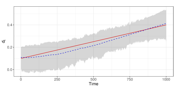
Figure 1: Result of 200 Monte Carlo simulations, where a time-varying fractional parameter (solid line) is estimated with a TV-FI model. The dashed line represent the average estimates, while the gray band shows the empirical 95% intervals.

In this Section, we carry out some Monte Carlo simulation experiments in order to establish if the proposed estimation method of the time-varying long-memory parameter $d$ performs well.

To demonstrate the performance of the proposed method, we simulated time series data, $y_{1},\ldots,y_{n},$ from two TV-FI process:

$$(1-B)^{d_{t}}\,y_{t}=\varepsilon_{t}\ ,$$ (8)

where $\varepsilon_{t}\sim iid\mathcal{N}(0,\sigma^{2}),$ and $d_{t}$ is defined, respectively, by:

$$d_{t}=0.1+0.3\ \frac{t}{n}$$ (9)

or

$$d_{t}=0.1+0.3\ \Phi\left(\frac{t-n/2}{3\,\sqrt{n}}\right)\ ,$$ (10)

with $\Phi(\cdot)$ indicating the standard Gaussian distribution function.

The first specification takes into account a slow increasing trend in $d_{t},$ while the second describes a slow change in regime of $d_{t},$ which changes from a short-memory to a persistent situation.

The evolution of $d_{t}$ is then estimated using the TV-FI model introduced above. It should be noted that in GAS models the scaling defined by (2) is often replaced by $S_{t}^{\gamma}$, for some suitable $\gamma$. We found results to be more stable with $\gamma=0.5$ (see also Creal et al., 2013). Also, GAS models can easily be accommodated in order to include a link function $\Lambda(\cdot)$, typically with the objective to constrain the parameter of interest to vary in some region. We used

$$d_{t}=\Lambda(g_{t})=a+(b-a)\ \frac{e^{g_{t}}}{1+e^{g_{t}}}\ ,$$

so that $d_{t}\in(a,b)$, while $g_{t}\in{\rm I\!R}$. Recursion (3) is then defined in terms of $g_{t}$, with (5) and (6) easily adjusted for the reparametrization.

It should be remarked that $d_{0}$, the value of the fractional parameter at time 0, is necessary to define the likelihood. We treated $d_{0}$ as a parameter to be estimated along with the others.

We obtained 200 Monte Carlo replications from the process defined by (8), and (9) or (10), setting $n=1000$ and $\sigma=2$.

For each replication, the TV-FI model was estimated by maximum likelihood, setting $(a,b)=(-0.4,0.6)$ and $\omega=0$, while estimating $(d_{0},\alpha,\beta,\sigma)$.

Simulation results are shown in Figure 1. The solid line shows the true evolution of $d_{t}$, while the dashed line is its estimate, averaged over the Monte Carlo replications. The gray band represents the empirical 95% intervals. Figure 1 shows how the TV-FI model is able to represent the evolution of the long-memory parameter, that would be completely missed by a model with constant $d$.

5 Empirical application

This Section provides two empirical applications of the proposed TV-FI model. First we describe the data and then present the empirical results.

5.1 Temperature anomalies

The first data set we analyze is the series of monthly global historical surface temperature anomalies relative to a 1961–1990 reference period, contained in the data set HadCRUT4. This dataset is a collaborative product of the Met Office Hadley Centre and the Climatic Research Unit at the University of East Anglia and contains data from January, 1850, to August, 2018, on a 5 degree grid, for a total of $n=2024$ observations (for all details about this dataset see Morice et al., 2012).

This series is very interesting since the earth is now in a period of rising global temperatures and some authors have considered the stochastic properties of univariate time series of both atmospheric and oceanic temperatures in an effort to estimate the natural variability of the earth’s climate. These series often exhibit the property of statistical long-memory (see Rea et al., 2011, and the references therein). If temperature series are long-memory, the implications for climatic change are that the temperature series are mean reverting. In this case, it is possible to support the idea that the observed rise in global temperatures represents a natural fluctuation which will reverse in the future.

Actually, the majority of the available studies could not establish the presence of true long-memory in the temperature series because the finite sample properties of both long-memory series and series with structural breaks (Sibbertsen, 2004). Moreover, Rea et al. (2011) conclude that none of the temperature series considered in their paper are true long-memory series, but that the series are non stationary because of structural changes.

Since changes might concern the fractional parameter $d$, we think that these are interesting series to apply the model we propose.

5.2 Euro-dollar exchange rate

The second series we consider is the financial time series of the daily euro-dollar exchange rate from January 1st, 2001, to November 20th, 2018, for a total of $n=4667$ observations .

The return series is defined as $x_{t}=\ln p_{t}-\ln p_{t-1}$, $t=2,\ldots n$, where $p_{t}$ is the closing quotation of the euro-dollar exchange rate. Our series of interest is given by the centered absolute returns $r_{t}=|x_{t}-\bar{x}|$, where $\bar{x}$ is the sample mean of $x_{t}$, as this series is a good proxy of the volatility. In fact (Cotter, 2011 and references therein) absolute returns are robust in the presence of extreme or tail movements; accurate measures of unobservable latent volatility are obtained from absolute return volatility asymptotically through the theoretical framework of realized power variation and, moreover, absolute return volatility gives desirable finite sample properties that are applicable in practice for the risk manager.

5.3 Predictive performance evaluation

The adequacy of the TV-FI model for the time series at hand is assessed by evaluating its predictive performance. Since GAS models are based on parametric assumptions, it is natural to consider predictions in the form of density forecasts (for reviews on probabilistic forecasting see e.g. Tay and Wallis, 2000, Timmermann, 2000, Gneiting, 2008 and Gneiting and Katzfuss, 2014). In particular, the one-step ahead predictive distributions ($h=1$) are analytically available, while in the multi-step ahead case ($h>1$) they need to be estimated by simulation. The diagnostic approach used here is the one based on the maximization of the sharpness of the predictive distribution, subject to calibration, as proposed by Gneiting et al. (2007). The predictive performance of the TV-FI model is compared to that of a FI$(d)$ model, with constant $d$, using proper scoring rules. A popular choice is the continuous ranked probability score (CRPS), defined as

$$\int_{-\infty}^{\infty}(F(y)-\mathds{1}\{y\leq z\})^{2}\,dz\ ,$$

where $F$ is the predictive CDF (Matheson and Winkler, 1976). Alternative representations of the CRPS, useful e.g. when $F$ is represented by a sample or when specific regions of interest need to be emphasized, are discussed in Gneiting and Raftery (2007) and Gneiting and Ranjan (2011). Another popular scoring rule is the logarithmic score, which for the observation $y$ is defined as $-\log(f(y))$, where $f$ is the predictive density (Good, 1852; Bernardo, 1979). However, this rule lacks robustness (Selten, 1998; Gneiting and Raftery, 2007), especially for multi-step ahead predictions ($h>1$), when the density (rather than the CDF required by the CRPS) needs to be estimated, typically with kernel density estimation. The estimated score may be highly sensitive to the choice of bandwidth, thus making the ranking of prediction methods more fragile. For these reasons, the following evaluations will be based on CRPS.

Formal statistical tests of equal predictive performance were also applied. In particular, we used the Diebold and Mariano (1995) test

$$\mbox{DM}_{l}=\sqrt{l}\ \frac{\bar{S}^{TV-FI}_{l}-\bar{S}^{FI(d)}_{l}}{\hat{\sigma}_{l}}\ ,$$ (11)

where $l$ is the length of the out-of-sample period, $\bar{S}^{M}$ represents the average score for model $M$ and $\hat{\sigma}^{2}_{l}$ is a suitable estimator of the asymptotic variance of the score difference. Under the null hypothesis of no difference between the expected scores, under regularity conditions the test statistic DM_l is asymptotically standard normal (Diebold and Mariano, 1995; Giacomini and White, 2006; Diebold, 2015). Concerning $\hat{\sigma}^{2}_{l}$, we follow Diks and Van Dijk (2011) in using the heteroskedasticity and autocorrelation consistent (HAC) estimator defined as

$$\hat{\sigma}^{2}_{l}=\hat{\gamma}_{0}+2\,\sum_{j=1}^{J}\left(1-\frac{j}{J}\right)\,\hat{\gamma}_{j}\ ,$$

where $J$ is the largest integer less than or equal to $l^{1/4}$ and $\hat{\gamma}_{j}$ is the lag $j$ sample autocovariance of the sequence $S_{1}^{TV-FI}-S_{1}^{FI(d)},\ldots,S_{l}^{TV-FI}-S_{l}^{FI(d)}$ of score differences over the out-of-sample period.

5.4 Results for temperature anomalies

Figure 2 reports the plot of the series together with its empirical autocorrelation function and the raw spectrum. From these plots it is evident that both the slow decaying behavior of the autocorrelation and the pole near the zero frequency are present, thus confirming the existence of long-memory behavior. The ADF test rejects the null hypothesis of unit root; moreover, the maximum likelihood estimate of the long-memory parameter $d$ calculated for the whole series is $0.498$, a very high value but lower than $0.5$. It is also evident that since (about) 1920 the series presents a slow but increasing trend and that since (about) 1980 the slope of this trend is greater. We want to investigate whether the model we propose is able to represent this evolution with a dynamic long-memory parameter.

Figure 2: Temperature anomalies, Jan:1950–Aug:2018. Plot of the series, the ACF and the raw spectrum.

Figure 3 reports the results of our estimates, based on the whole series. In particular, the evolution of $d_{t}$ is compared to the asymptotic confidence interval for a constant $d$. It is possible to see that the evolution of $d_{t}$ is much greater than that implied by a constant $d$, with larger values in the second part of the considered period.

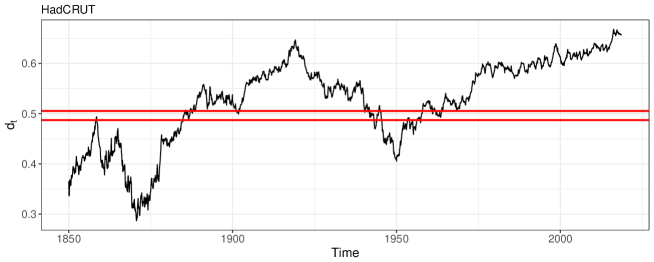
Figure 3: Temperature anomalies. Evolution of $d_{t}$ estimated with the TV-FI model, using the whole series. The horizontal band represents the asymptotic confidence interval for a constant $d$, also based on the whole series.

For the predictive performance evaluation, we estimated the TV-FI and FI$(d)$ models using the first 1000 observations (in-sample period). For the following out-of-sample period, we computed the conditional predictive distributions. The TV-FI and FI$(d)$ models are then compared according to their out-of sample performance, evaluated on the basis of the CRPS. Every 200 observations, models are re-estimated (and, therefore, the in-sample period extended).

The average out-of-sample scores for the two models are shown in Table 1. It should be reminded that models with a lower score generate more accurate predictions. Hence, the TV-FI model with dynamic $d$ has a better predictive performance than the FI$(d)$ with constant $d$, and especially so when the prediction horizon $h$ increases.

Prediction horizon $h$	1	2	3	6	9	12
Average CRPS: TV-FI	0.0575	0.0650	0.0709	0.0806	0.0870	0.0910
Average CRPS: FI$(d)$	0.0583	0.0664	0.0724	0.0830	0.0898	0.0946
DM test	-2.253	-2.640	-2.365	-2.709	-2.858	-3.442
$p$-value	0.012	0.004	0.009	0.003	0.002	0.000

Table 1: Temperature anomalies. Comparison of the predictive performances for the TV-FI and FI$(d)$ models across the out-of-sample period.

As can be seen from Table 1, the DM test (11) shows that our model with dynamic long-memory coefficient yields a significant improvement ($p$-values are for a one directional alternative) in the predictive performance, especially for longer prediction horizons.

Figure 4 sheds more light on this result, by showing the evolution, over the out-of-sample period, of the cumulative sum of the differences between the one-step prediction CRPS for the FI$(d)$ and TV-FI models (CS):

$$\mbox{CS}_{j}=\sum_{i=1}^{j}\left(S^{FI(d)}_{i}-S_{i}^{TV-FI}\right)\ ,\qquad j=1,\ldots,l,$$ (12)

where $S_{i}$ is the score for the $i$-th one-step prediction and $l$ is the length of the out-of-sample period. In Figure 4, periods when the TV-FI yields a more accurate forecast are represented by an upward slope. Interestingly, it can be seen that the TV-FI model with dynamic long-memory parameter outperforms the FI$(d)$ model after 1990, i.e. when an increase in the slope of temperature anomalies is observed.

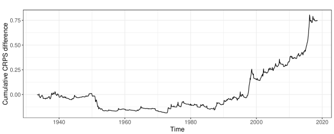
Figure 4: Temperature anomalies. Cumulative difference, in the out-of-sample period, between one-step prediction CRPS for the FI$(d)$ and TV-FI models.

5.5 Results for the euro-dollar exchange rate

We report in Figure 5 the observed series together with its empirical autocorrelation function and the raw spectrum. Even if the behavior of this series is completely different from the previous one, it is possible to see that also this series is characterized by the qualitative features typical of long-memory processes. The ADF test rejects the null hypothesis of unit root; moreover, the maximum likelihood estimate of the long-memory parameter $d$ calculated for the whole series is $0.131$, indicating that the effect of shocks is persistent over time.

Figure 5: Daily centered absolute log-returns of Euro-dollar exchange rates, 2001-01-01–2018-11-20. Plots of the series, the ACF and the raw spectrum.

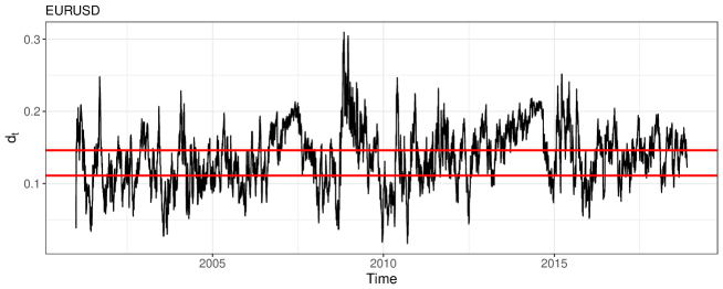
Figure 6: Centered absolute returns for the euro-dollar exchange rate. Evolution of $d_{t}$ estimated with the TV-FI model, using the whole series. The horizontal band represents the asymptotic confidence interval for a constant $d$, also based on the whole series.

Figure 6 reports the estimated evolution of $d_{t}$, compared to to the asymptotic confidence interval for a constant $d$, both based on the whole series. We see that the TV-FI model implies several periods in which the estimated $d_{t}$ remains above the asymptotic confidence interval.

Concerning the predictive performance, as for temperature anomalies the conditional predictive distribution are computed after estimating the TV-FI and FI$(d)$ models with the first 1000 observations (in-sample period) and updating model estimates every 200 observations.

The average out-of-sample scores for the two models are shown in Table 2. We see that only for $h=1$ the TV-FI and FI$(d)$ models have the same performance, while for $h>1$ using a dynamic $d$ improves significantly the predictive performance. This improvement increases with the prediction horizon $h$.

Prediction horizon $h$	1	2	3	6	9	12
Average CRPS: TV-FI	2.0920	2.0846	2.0874	2.0938	2.0974	2.1003
Average CRPS: FI$(d)$	2.0998	2.1031	2.1040	2.1154	2.1188	2.1243
DM test	-1.127	-2.593	-2.577	-3.416	-3.892	-4.616
$p$-value	0.130	0.005	0.005	0.000	0.000	0.000

Table 2: Centered absolute returns for the euro-dollar exchange rate. Comparison of the predictive performances for the TV-FI and FI$(d)$ models across the out-of-sample period (the average CRPS is multiplied by 1000 to facilitate comparison).

Figure 7 shows the evolution of CS_j, defined in equation (12) over the out-of-sample period. Upward slopes represent periods in which the TV-FI model outperforms the the FI$(d)$ model. Hence, after 2007 and after 2014 we see that the TV-FI model forecasts more accurately. Interestingly, these are the periods in which a sharp increase in the volatility of the EUR-USD absolute returns is observed.

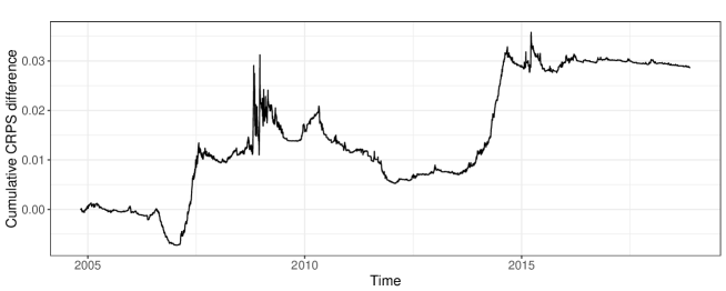
Figure 7: Centered absolute returns for the euro-dollar exchange rate. Cumulative difference, in the out-of-sample period, between one-step prediction CRPS for the FI$(d)$ and TV-FI models.

6 Conclusions

In this work we proposed a flexible time-varying fractionally integrated model which allows the long-memory parameter to vary dynamically over time. This model is based on the theory of Generalized Autoregressive Score (GAS) models by Creal et al. (2013) and Harvey (2013). The results we obtain are very promising for both simulated and real time series. In this work we consider only an FI model but future research may include the extension to a general ARFIMA$(p,d,q)$ even if, in our opinion, the varying long-memory parameter, $d_{t}$, is able to take into account also short memory components if present.

There are several future directions of research that could improve on the current work. Missing observations are often present in empirical studies, for example because unequally spaced time series are being considered or because stock prices are not recorded during holidays, despite the underlying values being changing due to external events. No simple solutions are available for missing observations in observations-driven models, like the GAS model considered here. However, the present work could be extended to a context with missing values by considering the results in Blasques et al. (2018), who use an indirect inference method to replicate the generating process of the time series. A different direction of research could concern the availability of intraday high-frequency data, that has led to the use of realized variance measures to improve the forecast of volatility, which is traditionally based, as in the present paper, on transformations of daily returns. Since realized variance measures are characterized by even stronger long memory than, e.g., squared daily returns (Andersen et al., 2001), it would be interesting to explore how this can be exploited in our modeling framework, possibly also using fractional integrated score dynamics as in Lucas and Opschoor (2016). From a more theoretical perspective, a closer link needs to be created with results on the consistency and asymptotic normality of maximum likelihood estimators for GAS models (Blasques et al., 2014a, b; Blasques et al., 2018).

7 Appendix

Using equation (4), we find

$$\nu_{j}(d_{t}) =\frac{\partial\pi_{j}(d_{t})}{\partial d_{t}}$$

$$=-d_{t}\ \frac{-\Gamma^{\prime}(j-d_{t})\,\Gamma(1-d_{t})\,\Gamma(j+1)+\Gamma^{\prime}(1-d_{t})\,\Gamma(j+1)\,\Gamma(j-d_{t})}{\left(\Gamma(1-d_{t})\,\Gamma(j+1)\right)^{2}}$$

$$-\frac{\Gamma(j-d_{t})}{\Gamma(1-d_{t})\,\Gamma(j+1)}$$

$$=\frac{-d_{t}\,\Gamma(j-d_{t})}{\Gamma(1-d_{t})\,\Gamma(j+1)}\left(\frac{-\Gamma^{\prime}(j-d_{t})}{\Gamma(j-d_{t})}+\frac{\Gamma^{\prime}(1-d_{t})}{\Gamma(1-d_{t})}+\frac{1}{d_{t}}\right)$$

$$=\pi_{j}(d_{t})\left(-\Psi(j-d_{t})+\Psi(1-d_{t})+\frac{1}{d_{t}}\right)\ ,$$

where $\Psi(\cdot)=\Gamma^{{}^{\prime}}(\cdot)/\Gamma(\cdot)$ is the digamma function. Therefore:

$$\nabla_{t} =-\frac{1}{\sigma^{2}}\left(y_{t}+\sum_{j=1}^{t-1}\pi_{j}(d_{t})\,y_{t-j}\right)\left(\sum_{j=1}^{t-1}\frac{\partial\pi_{j}(d_{t})}{\partial d_{t}}\,y_{t-j}\right)$$

$$=-\frac{1}{\sigma^{2}}\left(y_{t}+\sum_{j=1}^{t-1}\pi_{j}(d_{t})\,y_{t-j}\right)\left(\sum_{j=1}^{t-1}\nu_{j}(d_{t})\,y_{t-j}\right).$$

Now, observe that:

$$\frac{\partial^{2}\pi_{j}(d_{t})}{\partial d_{t}} =\nu_{j}(d_{t})\left[-\Psi(j-d_{t})+\Psi(1-d_{t})+\frac{1}{d_{t}}\right]$$

$$+\pi_{j}(d_{t})\left[\Psi^{{}^{\prime}}(j-d_{t})-\Psi^{{}^{\prime}}(1-d_{t})-\frac{1}{d^{2}_{t}}\right]\ .$$

Hence, we find

$$\mathcal{I}_{t-1}=-E_{t-1}\!\!\left[\frac{\partial\nabla_{t}}{\partial d_{t}}\right] =\frac{1}{\sigma^{2}}\,E_{t-1}\!\!\left[\left(\sum_{j=1}^{t-1}\nu_{j}(d_{t})\,y_{t-j}\right)^{2}\right.$$

$$+\left.\left(y_{t}+\sum_{j=1}^{t-1}\pi_{j}(d_{t})\,y_{t-j}\right)\left(\sum_{j=1}^{t-1}\frac{\partial^{2}\pi_{j}(d_{t})}{\partial d_{t}}\,y_{t-j}\right)\right]$$

$$=\frac{1}{\sigma^{2}}\,\left(\sum_{j=1}^{t-1}\nu_{j}(d_{t})\,y_{t-j}\right)^{2}\ ,$$

where we used $E_{t-1}\!\left[y_{t}+\sum_{j=1}^{t-1}\pi_{j}(d_{t})\,y_{t-j}\right]=E_{t-1}\!\left[\epsilon_{t}\right]=0$. Finally:

$$S_{t}=\mathcal{I}_{t-1}^{-1}=\sigma^{2}\,\left(\sum_{j=1}^{t-1}\nu_{j}(d_{t})\,y_{t-j}\right)^{-2}\ .$$

References

- Andersen et al. (2001) Andersen, T. G., T. Bollerslev, F. X. Diebold, and P. Labys (2001). The distribution of realized exchange rate volatility. Journal of the American Statistical Association 96(453), 42–55.
- Beran and Terrin (1996) Beran, J. and N. Terrin (1996). Testing for a change of the long-memory parameter. Biometrika 83, 627–638.
- Bernardo (1979) Bernardo, J. (1979). Expected information as expected utility. The Annals of Statistics 7(3), 686–690.
- Blasques et al. (2018) Blasques, F., P. Gorgi, and S. J. Koopman (2018). Missing observations in observation-driven time series models. Tinbergen Institute Discussion Papers, 2018-013/III.
- Blasques et al. (2018) Blasques, F., P. Gorgi, S. J. Koopman, and O. Wintenberger (2018). Feasible invertibility conditions and maximum likelihood estimation for observation-driven models. Electronic Journal of Statistics 12(1), 1019–1052.
- Blasques et al. (2014a) Blasques, F., S. J. Koopman, and A. Lucas (2014a). Maximum likelihood estimation for correctly specified generalized autoregressive score models: Feedback effects, contraction conditions and asymptotic properties. Tinbergen Institute Discussion Papers, 14-074/III.
- Blasques et al. (2014b) Blasques, F., S. J. Koopman, and A. Lucas (2014b). Maximum likelihood estimation for score-driven models. Tinbergen Institute Discussion Papers, 14-029/III.
- Boubaker (2018) Boubaker, H. (2018). A generalized arfima model with smooth transition fractional integration parameter. Journal of Time Series Econometrics 10, 1–20.
- Boutahar et al. (2008) Boutahar, M., G. Dufrénot, and A. Péguin-Feissolle (2008). A simple fractionally integrated model with a time-varying long memory parameter . Computational Economics 31, 225–241.
- Caporin and Pres (2013) Caporin, M. and J. Pres (2013). Forecasting temperature indeces density with time-varying long-memory models. Journal of Forecasting 32, 339–352.
- Cotter (2011) Cotter, J. (2011). Absolute return volatility. Working Papers 200415, Geary Institute, University College Dublin.
- Creal et al. (2013) Creal, D., S. Koopman, and A. Lucas (2013). Generalized autoregressive score models with applications. Journal of Applied Econometrics 28, 777–795.
- Diebold (2015) Diebold, F. X. (2015). Comparing predictive accuracy twenty years later: A personal perspective on the use and abuse of diebold-mariano tests. Journal of Business & Economic Statistics 33(1), 1–9.
- Diebold and Mariano (1995) Diebold, F. X. and R. S. Mariano (1995). Comparing predictive accuracy. Journal of Business & Economic Statistics 13(3), 253–263.
- Diks and Van Dijk (2011) Diks, Cees, P. V. and D. Van Dijk (2011). Likelihood-based scoring rules for comparing density forecasts in tails. Journal of Econometrics 163(2), 215–230.
- Giacomini and White (2006) Giacomini, R. and H. White (2006). Tests of conditional predictive ability. Econometrica 74(6), 1545–1578.
- Gneiting (2008) Gneiting, T. (2008). Editorial: Probabilistic forecasting. Journal of the Royal Statistical Society Series A 171(2), 319–321.
- Gneiting et al. (2007) Gneiting, T., F. Balabdaoui, and A. E. Raftery (2007). Probabilistic forecasts, calibration and sharpness. Journal of the Royal Statistical Society Series B 69(2), 243–268.
- Gneiting and Katzfuss (2014) Gneiting, T. and M. Katzfuss (2014). Probabilistic forecasting. Annual review of statistics and its application 1, 125–151.
- Gneiting and Raftery (2007) Gneiting, T. and A. E. Raftery (2007). Strictly proper scoring rules, prediction, and estimation. Journal of the American Statistical Association 102(477), 359–378.
- Gneiting and Ranjan (2011) Gneiting, T. and R. Ranjan (2011). Comparing density forecasts using threshold- and quantile-weighted scoring rules. Journal of Business & Economic Statistics 29(3), 411–422.
- Good (1852) Good, I. (1852). Rational decisions. Journal of the Royal Statistical Society Series B 14(1), 107–114.
- Granger and Joyeux (1980) Granger, C. and R. Joyeux (1980). An introduction to long-range time series models and fractional differencing. Journal of Time Series Analysis 1, 15–30.
- Harvey (2013) Harvey, A. (2013). Dynamic Models for Volatility and Heavy Tails: With Applications to Financial and Economic Time Series. Cambridge: University Press.
- Hassler and Meller (2014) Hassler, U. and B. Meller (2014). Detecting multiple breaks in long memory the case of u.s. inflation. Empirical Economics 46, 653–680.
- Hosking (1981) Hosking, J. (1981). Fractional differencing. Biometrika 68, 165–176.
- Jensen and Whitcher (2000) Jensen, M. J. and B. Whitcher (2000). Time-varying long-memory in volatility: Detection and estimation with wavelets.
- Lu and Guegan (2011) Lu, Z. and D. Guegan (2011). Estimation of time-varying long memory parameter using wavelet method. Communications in Statistics - Simulation and Computation 40, 596–613.
- Lucas and Opschoor (2016) Lucas, A. and A. Opschoor (2016). Fractional integration and fat tails for realized covariance kernels and returns. Tinbergen Institute Discussion Papers, 2016-069/IV.
- Matheson and Winkler (1976) Matheson, J. E. and R. L. Winkler (1976). Scoring rules for continuous probability distributions. Management Science 22(10), 1087–1096.
- Morice et al. (2012) Morice, C., J. Kennedy, N. Rayner, and J. P.D. (2012). Quantifying uncertainties in global and regional temperature change using an ensemble of observational estimates: The hadcrut4 dataset. Journal of Geophysical Research 117, 1–22.
- Palma (2007) Palma, W. (2007). Long-memory time series. New Jersey: Wiley.
- Ray and Tsay (2002) Ray, B. and R. Tsay (2002). Bayesian methods for change-point detection in long-range dependent processes. Journal of Time Series Analysis 23, 687–705.
- Rea et al. (2011) Rea, W., M. Reale, and B. J. (2011). Long memory in temperature reconstructions. Climatic Change 107, 247–265.
- Roueff and von Sachs (2011) Roueff, F. and R. von Sachs (2011). Locally stationary long memory estimation. Stochastic Processes and their Applications 121, 813–844.
- Selten (1998) Selten, R. (1998). Axiomatic characterization of the quadratic scoring rule. Experimental Economics 1, 43–62.
- Sibbertsen (2004) Sibbertsen, P. (2004). Long memory versus structural breaks: an overview. Statistical Papers 45, 465–515.
- Tay and Wallis (2000) Tay, A. S. and K. F. Wallis (2000). Density forecasting: A survey. Journal of Forecasting 19(4), 235–254.
- Timmermann (2000) Timmermann, A. (2000). Density forecasting in economics and finance. Journal of Forecasting 19(4), 231–234.
- Yamaguchi (2011) Yamaguchi, K. (2011). Estimating a change point in the long memory parameter. Journal of Time Series Analysis 32, 304–314.