Abstract

We introduce a family of models for magnetic skyrmions in the plane for which infinitely many solutions can be given explicitly. The energy defining the models is bounded below by a linear combination of degree and total vortex strength, and the configurations attaining the bound satisfy a first order Bogomol’nyi equation. We give explicit solutions which depend on an arbitrary holomorphic function. The simplest solutions are the basic Bloch and Néel skyrmions, but we also exhibit distorted skyrmions and anti-skyrmions as well as line defects and configurations consisting of skyrmions and anti-skyrmions.

1 Introduction

Magnetic skyrmions are topologically non-trivial configurations which occur in certain magnetic materials. It was first observed in [1] that particular examples of such configurations are minimisers of natural energy expressions for the magnetisation vector. They have since then become the subject of intense study, both experimentally and theoretically, not least because of their potential use as information carriers in magnetic storage devices, see [2] for a review.

In this paper we use tools from gauge theory, complex analysis and differential geometry to introduce models for magnetic skyrmions which can be solved explicitly. The models are grounded in the physics of magnetic skyrmions and belong to the general class already considered in [1], with an energy expression consisting of a Dirichlet term, a Dzyaloshinskii-Moriya (DM) interaction energy [3, 4] and a potential combining Zeeman and easy plane anisotropy terms. However, our formulation reveals that, for critical values of the coupling constants, the models are of Bogomol’nyi type, which means that static solutions can be obtained by solving a first order partial differential equation. Moreover, this equation can be solved in terms of an arbitrary holomorphic function. Both the Bogomol’nyi property and the existence of an infinite family of explicit solutions are novel in the context of magnetic skyrmions.

Models of Bogomol’nyi type have historically played an important role in the study of topological solitons [5]. They require a particular choice of coupling constants, but their mathematical properties allow for a far more detailed and explicit study of the solitons and their dynamics than would be possible in the generic case. Intricate and surprising features of soliton dynamics such as shapes and symmetries of multi-soliton configurations or scattering behaviour were first observed in models of Bogomol’nyi type and later found in generic soliton models.

The focus of this paper is the mathematical structure of the critically coupled models for magnetic skyrmions, and we only begin to explore the properties of our solutions. However, even at this stage it is clear that our infinite family of solutions contains several of the configurations associated with the various phases of generic models [6, 7, 8], and that it illustrates elliptical deformations [9, 10] and the recently studied skyrmion bags [11] or ‘sacks’ [12].

The simplest topological soliton theory of Bogomol’nyi type is the $O(3)$-sigma model in the plane [13]. The basic field is a map from the plane to the sphere, and finiteness of the Dirichlet energy requires the field to tend to a constant at spatial infinity, and to extend to a map from sphere to sphere. Such maps have a topological and integer degree, which is physically interpreted as the soliton number. The energy is bounded below by a multiple of the absolute value of the degree, and this bound is attained by configurations which satisfy the first order Bogomol’nyi equation. In this particular case, the Bogomol’nyi equation requires the configuration to be a holomorphic or anti-holomorphic map to the Riemann sphere.

In analogy with the baby skyrme model [14], one would expect the inclusion of DM interactions, Zeeman potential and anisotropy terms inevitably to destroy the Bogomol’nyi property of the pure $O(3)$ sigma model. However, here we shall show that, with a careful choice of potential and for a one-parameter family of DM interaction terms, our models preserve the Bogomol’nyi property and can be solved in terms of a fixed anti-holomorphic and an arbitrary holomorphic map to the Riemann sphere. The fixed anti-holomorphic part turns out to be an analytical version of the usual Bloch or Néel magnetic skyrmions, but the holomorphic part is new.

Our family of models is introduced in Sect. 2, and the solutions are studied in Sect. 5. Readers primarily interested in the models and their solutions are invited to skip directly from Sect. 2 to Sect. 5. In the intervening sections we derive the Bogomol’nyi equation in two different ways. In Sect. 3, we write the theory as a non-abelian gauge theory with a fixed non-abelian gauge field and apply a trick for constructing gauged sigma models of Bogomol’nyi type introduced in [15]. In Sect. 4, we derive the Bogomol’nyi equation in complex stereographic coordinates and give the general solution in terms of fixed anti-holomorphic and an arbitrary holomorphic function. We show that, when that holomorphic function is rational, the energy is generically positive and quantised in multiples of $4\pi$. We also point out that the energy is not well-defined when the leading holomorphic term at spatial infinity is linear, and propose a regularisation which preserves the generic formula. We study detailed properties of rational solutions in Sect. 5. The final Sect. 6 contains our conclusion and a brief discussion of open questions.

2 The model

2.1 Energy and symmetry

The basic field in any mathematical model for magnetic skyrmions is the magnetisation vector, which in the planar and static case is a map $\boldsymbol{n}:\mathbb{R}^{2}\rightarrow S^{2}$. Here we consider models where the energy of a configuration is measured by the sum of three terms: the Dirichlet or Heisenberg energy (quadratic in derivatives), a generalised DM interaction energy (linear in derivatives), and a potential term which may involve linear or quadratic terms in the Cartesian components of $\boldsymbol{n}=(n_{1},n_{2},n_{3})^{t}$ (with the constraint $n_{1}^{2}+n_{2}^{2}+n_{3}^{2}=1$ always understood). General models of this sort were considered in the seminal paper [1] in which the possibility of topologically stable configurations now known as magnetic skyrmions was first pointed out, and have been widely studied since then.

Our one-parameter family of models belongs to the general family considered in [1] but requires a particular choice of coupling constants, which we call critical. The parameter in the family is an angle $\alpha\in[0,2\pi)$, and describes a generalised DM interaction term. In order to define this term, we need some additional notation.

We use Cartesian coordinates $x_{1}$ and $x_{2}$ in the plane and write $\partial_{1}$ and $\partial_{2}$ for partial derivatives with respect to them. Thinking of $\mathbb{R}^{2}$ as embedded in Euclidean $\mathbb{R}^{3}$ and using three-dimensional notation, we also write $\boldsymbol{e}_{1},\boldsymbol{e}_{2},\boldsymbol{e}_{3}$ for the canonical basis of $\mathbb{R}^{3}$, with $\boldsymbol{e}_{3}=\boldsymbol{e}_{1}\times\boldsymbol{e}_{2}$. In terms of the rotation $R(\alpha)$ about the 3-axis by $\alpha\in[0,2\pi)$, we define

$$\boldsymbol{e}_{1}^{\alpha}=R(\alpha)\boldsymbol{e}_{1}=\begin{pmatrix}\cos\alpha\\ \sin\alpha\\ 0\end{pmatrix},\qquad\boldsymbol{e}_{2}^{\alpha}=R(\alpha)\boldsymbol{e}_{2}=\begin{pmatrix}-\sin\alpha\\ \phantom{-}\cos\alpha\\ 0\end{pmatrix},\qquad\boldsymbol{e}_{3}=\begin{pmatrix}0\\ 0\\ 1\end{pmatrix}.$$ (2.1)

Extending the usual definition of the gradient $\nabla=\sum_{i=1}^{2}\boldsymbol{e}_{i}\partial_{i}$ to write

$$\nabla_{\alpha}=\sum_{i=1}^{2}\boldsymbol{e}_{i}^{\alpha}\partial_{i},$$ (2.2)

and defining

$$\boldsymbol{n}^{\alpha}=R(\alpha)\boldsymbol{n},$$ (2.3)

the family of DM interaction terms we are interested in is

$$\boldsymbol{n}^{\alpha}\cdot\nabla\times\boldsymbol{n}^{\alpha}=\boldsymbol{n}\cdot\nabla_{-\alpha}\times\boldsymbol{n}.$$ (2.4)

In components, it consist of two familiar parts:

$$\boldsymbol{n}\cdot\nabla_{-\alpha}\times\boldsymbol{n}=\cos\alpha\;w_{B}+\sin\alpha\;w_{N},$$ (2.5)

where $w_{b}$ and $w_{N}$ are the following contractions of the chirality tensor $\boldsymbol{n}\times\partial_{i}\boldsymbol{n}$:

$$w_{B} =\phantom{-}n_{1}\partial_{2}n_{3}-n_{2}\partial_{1}n_{3}+n_{3}(\partial_{1}n_{2}-\partial_{2}n_{1}),$$

$$w_{N} =-n_{1}\partial_{1}n_{3}-n_{2}\partial_{2}n_{3}+n_{3}(\partial_{1}n_{1}+\partial_{2}n_{2}).$$ (2.6)

Choosing energy units so that the coefficient of the Dirichlet energy term is unity, the family of energy functionals we want to consider is

$$E[\boldsymbol{n}]=\int_{\mathbb{R}^{2}}\frac{1}{2}(\nabla\boldsymbol{n})^{2}+\kappa\boldsymbol{n}\cdot\nabla_{-\alpha}\times\boldsymbol{n}+\frac{\kappa^{2}}{2}(1-n_{3})^{2}\;\mathrm{d}x_{1}\mathrm{d}x_{2}.$$ (2.7)

The coupling constant $\kappa$ could also be set to unity by a choice of length unit, but we find it convenient to keep it in our calculations. We assume $\kappa>0$ for the remainder of this paper. Since

$$\frac{1}{2}(1-n_{3})^{2}=(1-n_{3})-\frac{1}{2}(1-n_{3}^{2}),$$ (2.8)

our potential term combines a Zeeman and easy plane anisotropy potential, with coefficients chosen in such a way that the sum is a perfect square.

The energy expression (2.7) is invariant under translations in the plane and under the group $O(2)$ of rotations and reflection of the plane, combined with simultaneous rotations and reflections of the target sphere. On fields, the rotations act as

$$\boldsymbol{n}(x_{1},x_{2})\mapsto R(\sigma)\boldsymbol{n}(\cos\sigma\,x_{1}-\sin\sigma\,x_{2},\sin\sigma\,x_{1}+\cos\sigma\,x_{2}),\quad\sigma\in[0,2\pi),$$ (2.9)

and the generator of reflections acts as

$$\boldsymbol{n}(x_{1},x_{2})\mapsto R(2\gamma)\bar{\boldsymbol{n}}(x_{1},-x_{2}),\quad\text{with}\quad\bar{\boldsymbol{n}}=\begin{pmatrix}\phantom{-}n_{1}\\ -n_{2}\\ \phantom{-}n_{3}\end{pmatrix}\quad\text{and}\quad\gamma=\frac{\pi}{2}-\alpha.$$ (2.10)

The symmetry group is smaller than that of generic baby skyrme models [14] because the DM interaction breaks the product of the orthogonal groups in space and target space to a diagonal subgroup. It is worth noting that it would be mathematically natural to consider an alternative version of the DM interaction with the opposite chirality:

$$\bar{\boldsymbol{n}}\cdot\nabla_{-\alpha}\times\bar{\boldsymbol{n}}.$$ (2.11)

If this term was used instead of the standard DM interaction, the symmetry would consist of spatial rotations as in (2.9) but combined with rotations $R(-\sigma)$ of $\boldsymbol{n}$. Both the DM interaction term (2.4) and the flipped version (2.11) were considered in [16], together with a generic linear combination of the Zeeman and anisotropy potential $(1-n_{3}^{2})$. We will work with the DM interaction (2.4) and primarily consider the critical linear combination (2.8), but we discuss the more general potential in Sect. 2.2 and comment on how our results would change if we had used the opposite chirality in the Conclusion.

At this point we should really specify which boundary conditions we impose on the field $\boldsymbol{n}$ at spatial infinity. It is a priori not clear if one should, as in the discussion of the $O(3)$ sigma model, consider only configurations which extend to continuous maps $S^{2}\rightarrow S^{2}$. If they did, then

$$Q[\boldsymbol{n}]=\frac{1}{4\pi}\int_{\mathbb{R}^{2}}\boldsymbol{n}\cdot\partial_{1}\boldsymbol{n}\times\partial_{2}\boldsymbol{n}\;\mathrm{d}x_{1}\mathrm{d}x_{2}$$ (2.12)

would automatically be an integer, giving the degree of the extended map.

As we shall see, we should in fact allow for configurations which do not have a continuous extension $S^{2}\rightarrow S^{2}$. Such maps do not have a topological degree, but the integral expression for $Q$ still plays an important role. We will refer to it as the degree throughout this paper.

In our model, the degree occurs invariably in conjunction with a term which also depends on the boundary behaviour, namely the total vortex strength

$$\Omega[\boldsymbol{n}]=\frac{1}{4\pi}\int_{\mathbb{R}^{2}}\omega\;\mathrm{d}x_{1}\mathrm{d}x_{2},$$ (2.13)

where the integrand is the vorticity of the first two components of $\boldsymbol{n}^{\alpha}$:

$$\omega=\kappa(\partial_{1}n_{2}^{\alpha}-\partial_{2}n_{1}^{\alpha}).$$ (2.14)

The expressions we have given for the total energy, the degree and the total vortex strength should all be interpreted as functionals on the space of magnetisation fields. For some magnetisation fields $\boldsymbol{n}$, the relevant integrals may not be well-defined. One might therefore want to restrict the following discussion to a class of configurations which have a well-defined total energy, total vortex strength and degree. However, as we shall see, it is impossible to do this without discarding some of the most interesting configurations which arise as solutions in our model. In order to keep the discussion general but also mathematically rigorous, we therefore need notation for the restrictions of the integrals (2.7),(2.12) and (2.13) to compact subsets $D\subset\mathbb{R}^{2}$. We define

$$E_{D}[\boldsymbol{n}] =\int_{D}\frac{1}{2}(\nabla\boldsymbol{n})^{2}+\kappa\boldsymbol{n}\cdot\nabla_{-\alpha}\times\boldsymbol{n}+\frac{\kappa^{2}}{2}(1-n_{3})^{2}\;\mathrm{d}x_{1}\mathrm{d}x_{2},$$

$$Q_{D}[\boldsymbol{n}] =\frac{1}{4\pi}\int_{D}\boldsymbol{n}\cdot\partial_{1}\boldsymbol{n}\times\partial_{2}\boldsymbol{n}\;\mathrm{d}x_{1}\mathrm{d}x_{2},$$

$$\Omega_{D}[\boldsymbol{n}] =\frac{1}{4\pi}\int_{D}\omega\;\mathrm{d}x_{1}\mathrm{d}x_{2},\qquad\qquad\qquad D\subset\mathbb{R}^{2}.$$ (2.15)

Clearly, $\omega\,\mathrm{d}x_{1}\wedge\mathrm{d}x_{2}=\mathrm{d}\Theta$, where

$$\Theta=\kappa(n_{1}^{\alpha}\mathrm{d}x_{1}+n_{2}^{\alpha}\mathrm{d}x_{2})$$ (2.16)

is a differential one-form which plays a central role in this paper. It then follows that

$$\Omega_{D}[\boldsymbol{n}]=\frac{1}{4\pi}\int_{\partial D}\Theta.$$ (2.17)

In particular, one can take $D$ to be a disk of radius $R$ and centred at the origin, so that $\partial D=C^{R}$ is the circle of radius $R$. For some of the configurations we consider, the limit

$$\Omega^{\circ}[\boldsymbol{n}]=\frac{1}{4\pi}\lim_{R\rightarrow\infty}\int_{C^{R}}\Theta$$ (2.18)

exists even when the integral defining $\Omega[\boldsymbol{n}]$ does not. We will treat $\Omega^{\circ}[\boldsymbol{n}]$ as a regularised total vortex strength in those cases. When $\Omega$ is well-defined it necessarily coincides with $\Omega^{\circ}$.

For the solutions we construct in this paper, the total vortex strength is generically well-defined and finite, and, as a consequence, the total energy turns out to be given by a simple formula. The regularisation (2.18) is such that the resulting regularised energy for the non-generic solutions naturally fits into this general formula. However, we should stress that the regularisation procedure is not essential for our main results..

Postponing a more detailed discussion of allowed configurations and topological invariants to Sect. 4 and the Conclusion, we now derive the variational equation for (2.7), only assuming that $\boldsymbol{n}$ is twice differentiable. By considering the variation $\delta\boldsymbol{n}=\boldsymbol{\epsilon}\times\boldsymbol{n}$ for an infinitesimal vector function $\boldsymbol{\epsilon}$ which vanishes rapidly at spatial infinity, we obtain

$$2\kappa(\boldsymbol{n}\cdot\nabla_{-\alpha})\boldsymbol{n}=\left(\Delta\boldsymbol{n}+\kappa^{2}(1-n_{3})\boldsymbol{e}_{3}\right)\times\boldsymbol{n}.$$ (2.19)

We will show that this equation is in fact implied by a first order equation.

2.2 Hedgehog fields

In the skyrmion literature, the magnetisation $\boldsymbol{n}$ is often described in terms of spherical polar coordinates, defined via

$$\boldsymbol{n}=\begin{pmatrix}\sin\theta\cos\phi\\ \sin\theta\sin\phi\\ \cos\theta\end{pmatrix},$$ (2.20)

where $\theta$ and $\phi$ are functions on the plane. This parametrisation is particularly useful when considering hedgehog fields. By definition, and using polar coordinates $(r,\varphi)$ in the plane, hedgehog fields have a profile $\theta$ which depends on $r$ only and a longitudinal angle $\phi$ which is related to $\varphi$ according to

$$\phi=\varphi+\gamma,$$ (2.21)

for a constant angle $\gamma$. Such fields are invariant under the rotational symmetry (2.9). They are additionally invariant under the reflection symmetry (2.10) if and only if we choose $\gamma$ to be the complementary angle of $\alpha$ as in (2.10), and we now make this choice. With the boundary condition

$$\theta(0)=\pi,\qquad\theta(\infty)=0,$$ (2.22)

one checks that hedgehog fields have degree $Q=-1$.

Before developing the general machinery for generating solutions of the equation (2.19), we note some properties of the much simpler hedgehog solutions in our model. We do this in a slightly more general family of models, obtained from (2.7) by replacing

$$\frac{\kappa^{2}}{2}(1-n_{3})^{2}\rightarrow\frac{\mu^{2}}{2}(1-n_{3})^{2}$$ (2.23)

for a further real constant $\mu$. Minimisers of the resulting energy functional were studied in [17], and those of degree $Q=-1$ were shown to have holomorphicity properties similar to the ones which we will demonstrate more generally for stationary points of (2.7). We will exhibit these properties in our discussion of example solutions in Sect. 5. Here we derive the profile of hedgehog solutions by a more pedestrian method.

For hedgehog fields and $\gamma=\frac{\pi}{2}-\alpha$, the energy expression with the replacement (2.23) is

$$E=2\pi\int_{0}^{\infty}rdr\left(\frac{1}{2}\left(\frac{d\theta}{dr}\right)^{2}+\frac{\sin^{2}\theta}{2r^{2}}+\kappa\left(\frac{d\theta}{dr}+\frac{\sin(2\theta)}{2r}\right)+\frac{\mu^{2}}{2}(1-\cos\theta)^{2}\right).$$ (2.24)

The Euler-Lagrange equation is

$$\frac{d^{2}\theta}{dr^{2}}=-\frac{1}{r}\frac{d\theta}{dr}+\frac{\sin(2\theta)}{2r^{2}}-2\kappa\frac{\sin^{2}\theta}{r}+\mu^{2}\sin\theta(1-\cos\theta).$$ (2.25)

With the boundary condition (2.22), this is solved by

$$\theta=2\tan^{-1}\left(\frac{2\kappa}{\mu^{2}r}\right).$$ (2.26)

As already advertised, we will recover this profile from the simplest solution of a first order Bogomol’nyi equation in the case $\mu=\kappa$ in equation (5.2) .

3 A Bogomol’nyi equation for magnetic skyrmions

We will now show that the energy functional (2.7) can be written as the sum of a squared expression and a linear combination of the integral expression for the degree (2.12) and the total vortex strength (2.13). The vanishing of the squared expression gives a first order Bogomol’nyi equation which implies the variational second order equation (2.19).

Our derivation of the Bogomol’nyi equation is inspired by a similar treatment of gauged sigma models in [15] and [18]. As noticed in [19], the combination

$$\partial_{i}\boldsymbol{n}-\kappa\boldsymbol{e}_{i}\times\boldsymbol{n},\qquad i=1,2,$$ (3.1)

which occurs in many calculations involving magnetic skyrmions and which is often called ‘helical derivative’ can be thought of as a covariant derivative with respect to a non-abelian gauge field. To see the benefits of this, we take a more general viewpoint and consider more general $su(2)$ gauge fields.

To minimise notation, we identify the $su(2)$ Lie algebra with $\mathbb{R}^{3}$ and the Lie algebra commutator with the vector product. Defining the covariant derivative of $\boldsymbol{n}$ as

$$D_{i}\boldsymbol{n}=\partial_{i}\boldsymbol{n}+\boldsymbol{A}_{i}\times\boldsymbol{n},$$ (3.2)

and the non-abelian field strength

$$\boldsymbol{F}_{ij}=\partial_{i}\boldsymbol{A}_{j}-\partial_{i}\boldsymbol{A}_{j}+\boldsymbol{A}_{i}\times\boldsymbol{A}_{j},\qquad i,j=1,2,$$ (3.3)

we note

$$(D_{1}\boldsymbol{n}+\boldsymbol{n}\times D_{2}\boldsymbol{n})^{2}=(D_{1}\boldsymbol{n})^{2}+(D_{2}\boldsymbol{n})^{2}-2D_{1}\boldsymbol{n}\times D_{2}\boldsymbol{n}\cdot\boldsymbol{n}.$$ (3.4)

and also, as already observed by ’t Hooft [20],

$$\boldsymbol{n}\cdot D_{1}\boldsymbol{n}\times D_{2}\boldsymbol{n}-\boldsymbol{n}\cdot\boldsymbol{F}_{12}=\boldsymbol{n}\cdot\partial_{1}\boldsymbol{n}\times\partial_{2}\boldsymbol{n}+\partial_{2}(\boldsymbol{n}\cdot\boldsymbol{A}_{1})-\partial_{1}(\boldsymbol{n}\cdot\boldsymbol{A}_{2}).$$ (3.5)

This equation shows that the particular combination of the degree density (the integrand of (2.12)) with a two-dimensional curl on the right hand side can be expressed in a manifestly gauge invariant way.

We can now state and prove the main result in this section.

Lemma 3.1.

The energy for magnetic skyrmions at critical coupling associated with a compact subset $D\subset\mathbb{R}^{2}$ can be written as

$$E_{D}[\boldsymbol{n}]=4\pi(Q_{D}[\boldsymbol{n}]+\Omega_{D}[\boldsymbol{n}])+\int_{D}(D_{1}\boldsymbol{n}+\boldsymbol{n}\times D_{2}\boldsymbol{n})^{2}\;\mathrm{d}x_{1}\mathrm{d}x_{2},$$ (3.6)

where we used the covariant derivative

$$D_{i}\boldsymbol{n}=\partial_{i}\boldsymbol{n}-\kappa\boldsymbol{e}_{i}^{-\alpha}\times\boldsymbol{n},\quad i=1,2,$$ (3.7)

defined in terms of (2.1). In particular, the equality

$$E_{D}[\boldsymbol{n}]=4\pi(Q_{D}[\boldsymbol{n}]+\Omega_{D}[\boldsymbol{n}])$$ (3.8)

holds for all compact subsets $D\subset\mathbb{R}$ iff the Bogomol’nyi equation

$$D_{1}\boldsymbol{n}=-\boldsymbol{n}\times D_{2}\boldsymbol{n}$$ (3.9)

is satisfied. This equation implies the variational equation (2.19).

Proof.

Consider the gauge field given by the constant, Lie algebra-valued one-form with Cartesian components

$$\boldsymbol{A}_{i}=-\kappa\boldsymbol{e}_{i}^{-\alpha},\qquad i=1,2.$$ (3.10)

Then

$$\boldsymbol{F}_{12}=\kappa^{2}\boldsymbol{e}_{3},\quad\boldsymbol{n}\cdot\boldsymbol{A}_{i}=-\kappa\boldsymbol{n}_{i}^{\alpha},\quad i=1,2,$$ (3.11)

and therefore combining the results (3.4) and (3.5) for this gauge field gives

$$(D_{1}\boldsymbol{n}+\boldsymbol{n}\times D_{2}\boldsymbol{n})^{2}=(D_{1}\boldsymbol{n})^{2}+(D_{2}\boldsymbol{n})^{2}-2\left(\boldsymbol{n}\cdot\partial_{1}\boldsymbol{n}\times\partial_{2}\boldsymbol{n}+\kappa(\partial_{1}n_{2}^{\alpha}-\partial_{2}n_{1}^{\alpha})+\kappa^{2}n_{3}\right).$$ (3.12)

One also checks that

$$\frac{1}{2}(D_{1}\boldsymbol{n}^{2}+D_{2}\boldsymbol{n}^{2})=\frac{1}{2}(\nabla\boldsymbol{n})^{2}+\kappa\boldsymbol{n}\cdot\nabla_{-\alpha}\times\boldsymbol{n}+\frac{1}{2}\kappa^{2}(1+n_{3}^{2}),$$ (3.13)

and so the energy density of (2.7) can be written as

$$\frac{1}{2}(\nabla\boldsymbol{n})^{2}+ \kappa\boldsymbol{n}\cdot\nabla_{-\alpha}\times\boldsymbol{n}+\frac{\kappa^{2}}{2}(1-n_{3})^{2}$$

$$=\frac{1}{2}(D_{1}\boldsymbol{n}+\boldsymbol{n}\times D_{2}\boldsymbol{n})^{2}+\boldsymbol{n}\cdot\partial_{1}\boldsymbol{n}\times\partial_{2}\boldsymbol{n}+\kappa(\partial_{1}n_{2}^{\alpha}-\partial_{2}n_{1}^{\alpha}).$$ (3.14)

Integrating and using the definitions (2.1), we deduce that the energy associated with a compact subset $D\subset R^{2}$ can be written as claimed in (3.6). The equality (3.8) holds for all $D\subset\mathbb{R}^{2}$ iff

$$D_{1}\boldsymbol{n}=-\boldsymbol{n}\times D_{2}\boldsymbol{n}\Leftrightarrow D_{2}\boldsymbol{n}=\boldsymbol{n}\times D_{1}\boldsymbol{n},$$ (3.15)

where the equivalence follows by applying $\boldsymbol{n}\times$.

Showing that the equation (3.15) implies the variational equation is a lengthy but standard calculation. We indicate the main steps. Spelling out the Bogomol’nyi equation, we have

$$\partial_{1}\boldsymbol{n} =-\boldsymbol{n}\times\partial_{2}\boldsymbol{n}+\kappa(\boldsymbol{e}_{1}^{-\alpha}\times\boldsymbol{n}+\boldsymbol{n}\times(\boldsymbol{e}^{-\alpha}_{2}\times\boldsymbol{n})),$$

$$\partial_{2}\boldsymbol{n} =\boldsymbol{n}\times\partial_{1}\boldsymbol{n}+\kappa(\boldsymbol{e}^{-\alpha}_{2}\times\boldsymbol{n}-\boldsymbol{n}\times(\boldsymbol{e}_{1}^{-\alpha}\times\boldsymbol{n})).$$ (3.16)

Therefore

$$\partial_{1}^{2}\boldsymbol{n}+\partial_{2}^{2}\boldsymbol{n}=2\partial_{2}\boldsymbol{n}\times\partial_{1}\boldsymbol{n}+\kappa(\boldsymbol{e}_{1}^{-\alpha}\times\partial_{1}\boldsymbol{n}+\boldsymbol{e}_{2}^{-\alpha}\times\partial_{2}\boldsymbol{n})$$

$$+\kappa(\partial_{1}\boldsymbol{n}\times(\boldsymbol{e}_{2}^{-\alpha}\times\boldsymbol{n})+\boldsymbol{n}\times(\boldsymbol{e}_{2}^{-\alpha}\times\partial_{1}\boldsymbol{n})-\partial_{2}\boldsymbol{n}\times(\boldsymbol{e}_{1}^{-\alpha}\times\boldsymbol{n}))-\boldsymbol{n}\times(\boldsymbol{e}_{1}^{-\alpha}\times\partial_{2}\boldsymbol{n})).$$ (3.17)

Taking a cross product with $\boldsymbol{n}$ and noting

$$\boldsymbol{n}\times(\boldsymbol{e}_{i}^{-\alpha}\times\partial_{j}\boldsymbol{n})=-n_{i}^{\alpha}\partial_{j}\boldsymbol{n},$$ (3.18)

we arrive at

$$\boldsymbol{n}\times\Delta\boldsymbol{n}=-\kappa(n_{1}^{\alpha}\partial_{1}+n_{2}^{\alpha}\partial_{2})\boldsymbol{n}+\kappa(n_{1}^{\alpha}\boldsymbol{n}\times\partial_{2}\boldsymbol{n}-n_{2}^{\alpha}\boldsymbol{n}\times\partial_{1}\boldsymbol{n}).$$ (3.19)

Now we use the Bogomol’nyi equation again in the last term to conclude that

$$\kappa(n_{1}^{\alpha}\boldsymbol{n}\times\partial_{2}\boldsymbol{n}-n_{2}^{\alpha}\boldsymbol{n}\times\partial_{1}\boldsymbol{n})=-\kappa(n_{1}^{\alpha}\partial_{1}+n_{2}^{\alpha}\partial_{2})\boldsymbol{n}+\kappa^{2}(1-n_{3})\boldsymbol{e}_{3}\times\boldsymbol{n}.$$ (3.20)

Therefore

$$\boldsymbol{n}\times\Delta\boldsymbol{n}=-2\kappa(n_{1}^{\alpha}\partial_{1}+n_{2}^{\alpha}\partial_{2})\boldsymbol{n}+\kappa^{2}(1-n_{3})\boldsymbol{e}_{3}\times\boldsymbol{n},$$ (3.21)

which is the equation (2.19) obtained by variation. ∎

As often in the $O(3)$ sigma model or its gauged versions, the Bogomol’nyi equations are best studied in complex, stereographic coordinates. We do this in the next section.

4 Magnetic skyrmions in complex coordinates

4.1 The Bogomol’nyi equation in stereographic coordinates

We use stereographic coordinates on the sphere defined by projection from the south pole. With the abbreviation

$$\nu=n_{1}+in_{2},$$ (4.1)

our stereographic coordinate is

$$w=\frac{\nu}{1+n_{3}}.$$ (4.2)

When the magnetisation tends to the minimum of the potential term, $\boldsymbol{n}\rightarrow(0,0,1)^{t}$, then $w\rightarrow 0$. This makes $w$ a natural choice of coordinate, but in describing our solutions we also need

$$v=\frac{1}{w}.$$ (4.3)

For later use we also note the inverse relation

$$\nu=\frac{2w}{1+|w|^{2}},\quad n_{3}=\frac{1-|w|^{2}}{1+|w|^{2}}.$$ (4.4)

We introduce the complex coordinate $z=x_{1}+ix_{2}$ in the plane, and use the standard holomorphic and anti-holomorphic derivatives

$$\partial_{z}=\frac{1}{2}(\partial_{1}-i\partial_{2}),\qquad\partial_{\bar{z}}=\frac{1}{2}(\partial_{1}+i\partial_{2}).$$ (4.5)

Observing that, with the notation (2.3), $e^{i\alpha}\nu=n_{1}^{\alpha}+in_{2}^{\alpha}$, the DM interaction term (2.4) can be written in stereographic coordinates as

$$\kappa\boldsymbol{n}\cdot\nabla_{-\alpha}\times\boldsymbol{n}=2\kappa\text{Im}(e^{i\alpha}(n_{3}\partial_{z}\nu-\nu\partial_{z}n_{3}))=4\kappa\text{Im}\left(e^{i\alpha}\frac{\partial_{z}w+w^{2}\partial_{z}\bar{w}}{(1+|w|^{2})^{2}}\right).$$ (4.6)

The other terms in the energy functional have standard expressions in stereographic coordinates, and so the energy (2.7) is

$$E[w]=\int_{\mathbb{R}^{2}}\frac{2|\nabla w|^{2}+4\kappa\text{Im}(e^{i\alpha}(\partial_{z}w+w^{2}\partial_{z}\bar{w}))+2\kappa^{2}|w|^{4}}{(1+|w|^{2})^{2}}\;\mathrm{d}x_{1}\mathrm{d}x_{2}.$$ (4.7)

The integral (2.12) defining the degree is

$$Q[w]=\frac{i}{2\pi}\int_{\mathbb{R}^{2}}\frac{\partial_{1}w\partial_{2}\bar{w}-\partial_{2}w\partial_{1}\bar{w}}{(1+|w|^{2})^{2}}\;\mathrm{d}x_{1}dx_{2},$$ (4.8)

while the vorticity (2.14) is

$$\omega=2\kappa\text{Im}(e^{i\alpha}\partial_{z}\nu)=4\kappa\text{Im}\left(e^{i\alpha}\frac{\partial_{z}w-w^{2}\partial_{z}\bar{w}}{(1+|w|^{2})^{2}}\right).$$ (4.9)

The one-form $\Theta$ can be written as

$$\Theta=\kappa\text{Re}(e^{-i\alpha}\bar{\nu}\mathrm{d}z)=\kappa\frac{2\text{Re}(e^{-i\alpha}\bar{w}\mathrm{d}z)}{1+|w|^{2}}=\kappa\frac{2\text{Re}(e^{-i\alpha}v\mathrm{d}z)}{1+|v|^{2}}.$$ (4.10)

In the following we write $E_{D}[w],Q_{D}[w]$ and $\Omega_{D}[w]$ for the integrals (2.1) over $D\subset\mathbb{R}^{2}$ with the integrands expressed in terms of the complex field $w$. We can now state the main result of this paper.

Theorem 4.1.

The energy (2.1) associated with a compact subset $D\subset\mathbb{R}^{2}$ can be written as

$$E_{D}[w]=4\pi(Q_{D}[w]+\Omega_{D}[w])+\int_{D}8\frac{(\partial_{\bar{z}}w-\frac{i}{2}\kappa e^{i\alpha}w^{2})(\partial_{z}\bar{w}+\frac{i}{2}\kappa e^{-i\alpha}\bar{w}^{2})}{(1+|w|^{2})^{2}}\,\mathrm{d}x_{1}\mathrm{d}x_{2}.$$ (4.11)

The equality

$$E_{D}[w]=4\pi(Q_{D}[w]+\Omega_{D}[w])$$ (4.12)

holds for all compact $D\subset\mathbb{R}^{2}$ iff the field $v$ defined in (4.3) satisfies the Bogomol’nyi equation

$$\partial_{\bar{z}}v=-\frac{i}{2}\kappa e^{i\alpha}.$$ (4.13)

The general solution is

$$v=-\frac{i}{2}\kappa e^{i\alpha}\bar{z}+f(z),$$ (4.14)

where $f$ is an arbitrary holomorphic map from the plane to the Riemann sphere.

Proof.

Using the standard identity

$$\partial_{z}\bar{w}\partial_{\bar{z}}w=\frac{1}{4}\left(|\partial_{1}w|^{2}+|\partial_{2}w|^{2}-i(\partial_{1}w\partial_{2}\bar{w}-\partial_{2}w\partial_{1}\bar{w})\right).$$ (4.15)

and the expression for the vorticity (4.9) in complex coordinates, we have the following identities for the energy density

$$\frac{2|\nabla w|^{2}+4\kappa\text{Im}(e^{i\alpha}(\partial_{z}w+w^{2}\partial_{z}\bar{w}))+2\kappa^{2}|w|^{4}}{(1+|w|^{2})^{2}}$$

$$=\omega+\frac{2|\nabla w|^{2}+8\kappa\text{Im}(e^{i\alpha}w^{2}\partial_{z}\bar{w})+2\kappa^{2}|w|^{4}}{(1+|w|^{2})^{2}}$$

$$=\omega+2i\frac{\partial_{1}w\partial_{2}\bar{w}-\partial_{2}w\partial_{1}\bar{w}}{(1+|w|^{2})^{2}}+\frac{8\partial_{z}\bar{w}\bar{\partial}w+8\kappa\text{Im}(e^{i\alpha}w^{2}\partial_{z}\bar{w})+2\kappa^{2}|w|^{4}}{(1+|w|^{2})^{2}}$$

$$=\omega+2i\frac{\partial_{1}w\partial_{2}\bar{w}-\partial_{2}w\partial_{1}\bar{w}}{(1+|w|^{2})^{2}}+8\frac{(\partial_{\bar{z}}w-\frac{i}{2}\kappa e^{i\alpha}w^{2})(\partial_{z}\bar{w}+\frac{i}{2}\kappa e^{-i\alpha}\bar{w}^{2})}{(1+|w|^{2})^{2}}.$$

Integrating and using the expression (4.8) yields the claimed expression (4.11) for the energy.

It follows immediately that the equality (4.12) holds for all compact $D\subset\mathbb{R}^{2}$ iff

$$\partial_{\bar{z}}w=\frac{i}{2}\kappa e^{i\alpha}w^{2},$$ (4.16)

which is the Bogomol’nyi equation (3.9) in complex coordinates. With $v$ as defined, this is equivalent to

$$\partial_{\bar{z}}v=-\frac{i}{2}\kappa e^{i\alpha},$$ (4.17)

whose general solution is $v=-\frac{i}{2}\kappa e^{i\alpha}\bar{z}+f(z)$, where $f$ is an arbitrary holomorphic function, as claimed. Since $f$ takes values in the Riemann sphere, it is allowed to take the value $\infty$. ∎

One checks that the equation (4.13) is equivalent to the Bogomol’nyi equation (3.9), and that it therefore implies the variational equation (2.19). For later use we note that the energy density of configurations which satisfy the Bogomol’nyi equation is the vorticity plus $4\pi$ times the integrand of the degree. This sum can be written as

$$\epsilon(x_{1},x_{2})=4\frac{\partial_{z}w\partial_{\bar{z}}\bar{w}-\partial_{\bar{z}}w\partial_{z}\bar{w}+\kappa\text{Im}\left(e^{i\alpha}(\partial_{z}w-w^{2}\partial_{z}\bar{w})\right)}{(1+|w|^{2})^{2}}.$$ (4.18)

4.2 Degree and vorticity of magnetic skyrmions at critical coupling

Before discussing the topology of the magnetic skyrmions defined by (4.14), it is worth revisiting the simpler case of the standard $O(3)$ sigma model in the plane, defined by the Dirichlet energy functional [13, 5]. The requirement of finite energy in that model leads to the condition that fields tend to a constant at spatial infinity and may be extended to smooth maps $S^{2}\rightarrow S^{2}$. The Bogomol’nyi equations are then equivalent to the map being either holomorphic or anti-holomorphic. Considering the holomorphic case for definiteness, the energy is proportional to the degree and for this to be finite, the configuration has to be a rational map, i.e., of the form $p(z)/q(z)$, where $p$ and $q$ are polynomials of degree $m$ and $n$. The topological degree of the map is simply max$(m,n)$ in that case.

The DM term, which is a crucial feature of all models of magnetic skyrmions, is not positive definite, and therefore the energy expression for magnetic skyrmions may be finite even for configurations which do not tend to a constant value at spatial infinity. As a result, even finite energy configurations do not necessarily extend to smooth maps $S^{2}\rightarrow S^{2}$ and do not necessarily have a well-defined topological degree. Moreover, it is not clear a priori if solutions of the Bogomol’nyi equation in our models have well-defined total vortex strength and total energy.

We shall now illustrate these issues for our infinite family of solutions (4.14), and show that, for rational maps $f$, the combination $4\pi(Q+\Omega^{0})$ of degree and the regularised total vortex strength (2.18) nonetheless always yields a positive integer multiple of $4\pi$.

Before we enter a general discussion, it is illuminating to consider linear examples of the form

$$v=-\frac{i}{2}\kappa e^{i\alpha}(\bar{z}+Ae^{i\chi}z),\qquad A\in\mathbb{R}^{\geq 0}.$$ (4.19)

As we shall see, this family captures the essence of the problem of defining the degree and the total vortex strength.

The evaluation of the integral defining $Q$ is elementary. Switching to polar coordinates according to $z=re^{i\varphi}$, we find, after completing the radial integration,

$$Q[w]=\frac{1}{2\pi}\int_{0}^{2\pi}\frac{A^{2}-1}{1+A^{2}+2A\cos(2\varphi+\chi)}\mathrm{d}\varphi.$$ (4.20)

The evaluation of the total vortex strength is more subtle. The one-form $\Theta$ for the field (4.19) is

$$\Theta=4\frac{(1+A\cos(2\varphi+\chi))\mathrm{d}\varphi+A\sin(2\varphi+\chi)\mathrm{d}\ln r}{r^{-2}+(1+A^{2}+2A\cos(2\varphi+\chi)}.$$ (4.21)

When computing the total vortex strength, we need to integrate this form over a curve along which $r$ is large. The leading term is

$$\Theta\sim 4\frac{(1+A\cos(2\varphi+\chi))}{1+A^{2}+2A\cos(2\varphi+\chi)}\mathrm{d}\varphi+4\frac{A\sin(2\varphi+\chi)}{1+A^{2}+2A\cos(2\varphi+\chi)}\mathrm{d}\ln r.$$ (4.22)

Clearly, the integral of the term proportional to $\mathrm{d}\varphi$ gives the same answer for any simple curve enclosing the origin. However, the integral of the term proportional to $A\;\mathrm{d}\ln r$ depends on the curve we choose, even in the limit of large radius. One can use the $\varphi$-dependence to introduce arbitrary contributions by deforming the contour with an outward bulge starting at some angle $\varphi_{1}$ and ending at $\varphi_{2}>\varphi_{1}$. We conclude that the total vortex strength is not well-defined for configurations defined by (4.19) when $A\neq 0$.

However, the integral of $\Theta$ along a large circle $C^{R}$ centred at the origin has a well-defined limit as the radius tends to infinity, precisely because $\mathrm{d}\ln r$ does not contribute along such a circle. Thus, with the definition (2.18)

$$\Omega^{0}[w]=\frac{1}{2\pi}\int_{0}^{2\pi}\frac{2+2A\cos(2\varphi+\chi)}{1+A^{2}+2A\cos(2\varphi+\chi)}\mathrm{d}\varphi.$$ (4.23)

It is immediate that

$$Q[w]+\Omega^{\circ}[w]=1,$$ (4.24)

regardless of the value of $A$. However, the contribution from the degree and the vortex strength depends crucially on $A$. Since

$$Q[w]=\frac{1}{2\pi}\int_{0}^{2\pi}\frac{A^{2}-1}{1+A^{2}+2A\cos(2\varphi+\chi)}\mathrm{d}\varphi=\begin{cases}\phantom{-}1\quad&\text{if}\quad A>1\\ \phantom{-}0\quad&\text{if}\quad A=1\\ -1\quad&\text{if}\quad A<1,\end{cases}$$ (4.25)

and

$$\Omega^{\circ}[w]=\frac{1}{2\pi}\int_{0}^{2\pi}\frac{2+2A\cos(2\varphi+\chi)}{1+A^{2}+2A\cos(2\varphi+\chi)}\mathrm{d}\varphi=\begin{cases}0\quad&\text{if}\quad A>1\\ 1\quad&\text{if}\quad A=1\\ 2\quad&\text{if}\quad A<1,\end{cases}$$ (4.26)

we see that a configuration dominated by the holomorphic part ($A>1$) has degree 1 and vanishing vortex strength. A configuration dominated by the anti-holomorphic part ($A<1$) has degree -1 but vortex strength 2. In the intermediate case $A=1$, the degree comes out as 0 and the vortex strength contributes 1.

The deeper reason behind the ‘jumping’ of the degree of the map defined by (4.19) lies in the extendibility of the map to one between spheres. An overall factor is irrelevant for this discussion, so we consider

$$v=\bar{z}+Ae^{i\chi}z.$$ (4.27)

Then $w=1/v$ has a pole when $re^{-2i\varphi}=-Are^{i\chi}$. This has no solution when $A\neq 1$, but is solved by the entire line

$$\varphi=-\frac{\chi}{2}\pm\frac{\pi}{2}$$ (4.28)

when $A=1$. In particular, $w$ therefore does not have a good limit for $z\rightarrow\infty$ when $A=1$: the result is infinity along the direction (4.28) but zero otherwise. It therefore does not extend to a smooth map between spheres in that case. When $A\neq 1$ one checks, by considering the map in terms of $\zeta=1/z$, that $w$ does extend to a smooth map between spheres. Our integrations confirm this analysis for $A\neq 1$, but also show that the combination of degree and vortex strength gives a stable result even when $A=1$.

Our observations about the examples (4.19) generalise. In order to formulate this generalisation we define the regularised energy of a solution of the Bogomol’nyi equation as

$$E^{\circ}[w]=4\pi(Q[w]+\Omega^{0}[w]).$$ (4.29)

Lemma 4.2.

If $p$ and $q$ are polynomials in $z$ of degree $m$ and $n$ and without common factor, the integral defining the total energy of the magnetic skyrmion solution determined via

$$v=-\frac{i}{2}\kappa e^{i\alpha}\bar{z}+\frac{p(z)}{q(z)},$$ (4.30)

is well-defined provided $m\neq n+1$, i.e., provided $p/q$ does not grow linearly for large $z$. The total energy is

$$E[w]=4\pi\;\text{max}(m,n+1)\qquad\text{if}\quad m\neq n+1.$$ (4.31)

When $m=n+1$, the total energy is not well-defined but the regularised total energy is

$$E^{\circ}[w]=4\pi\;m\qquad\text{if}\quad m=n+1.$$ (4.32)

Proof.

It is clear that

$$f(z)=\frac{p(z)}{q(z)}$$ (4.33)

is a holomorphic map to the Riemann sphere, so (4.30) defines a magnetic skyrmion satisfying the Bogomol’nyi equation. Written in terms of $v$, the energy density (4.18) is

$$\epsilon(x_{1},x_{2})=4\frac{\partial_{z}v\partial_{\bar{z}}\bar{v}-\partial_{\bar{z}}v\partial_{z}\bar{v}+\kappa\text{Im}\left(e^{i\alpha}(\partial_{z}\bar{v}-\bar{v}^{2}\partial_{z}v)\right)}{(1+|v|^{2})^{2}}.$$ (4.34)

This expression shows in particular that the energy density is smooth at the poles of $w$ (zeros of $v$), so that any divergence in the energy integral must come from the behaviour at infinity. We first show that there is no divergence when $m\neq n+1$.

For solutions of the form (4.30) and $m-n>1$, the leading term in the energy density for large $r$ comes from

$$4\kappa\frac{\text{Im}\left(-e^{i\alpha}\bar{v}^{2}\partial_{z}v\right)}{(1+|v|^{2})^{2}},$$ (4.35)

leading to the asymptotic formula

$$|\epsilon(r,\varphi)|=Cr^{-(m-n+1)}+\mathcal{O}\left(r^{-(m-n+2)}\right),\quad\text{for some}\;C\in\mathbb{R}.$$ (4.36)

This is integrable with respect to the integration measure $r\mathrm{d}r\,\mathrm{d}\varphi$ for $m-n>1$.

When $m-n<1$, the leading large-$r$ behaviour in the energy density is determined by the linear anti-holomorphic term in $v$, so the energy density behaves asymptotically as

$$|\epsilon(r,\varphi)|=Cr^{-4}+\mathcal{O}\left(r^{-5}\right),\quad\text{for some}\;C\in\mathbb{R}.$$ (4.37)

This is again integrable with respect to the integration measure $r\mathrm{d}r\,\mathrm{d}\varphi$.

Next we turn to the evaluation of the energy integral. Our calculations will also show that, for $m=n+1$, the integral requires regularisation. Our strategy is as follows. For any solution of the Bogomol’nyi equation we have $E_{D}[w]=4\pi(Q_{D}[w]+\Omega_{D}[w])$ for any compact subset $D\subset\mathbb{R}^{2}$. In order to evaluate the energy integral, we turn the integral defining the degree into boundary integrals and evaluate them together with the boundary integral defining the total vortex strength. In the cases where the total energy is well-defined, we will find that the boundary contribution from infinity is independent of the choice of contour at infinity. In the case where $p/q$ grows linearly at infinity, we evaluate the boundary contribution on a circle at infinity, leading to our result for the regularised energy.

We recall that the expression (2.12) for the degree is the integral of the pull-back of the area form on $S^{2}$, and that it can be written in terms of $w$ and $v$ as

$$4\pi Q[w]=2i\int_{\mathbb{R}^{2}}\frac{\mathrm{d}w\wedge\mathrm{d}\bar{w}}{(1+|w|^{2})^{2}}=2i\int_{\mathbb{R}^{2}}\frac{\mathrm{d}v\wedge\mathrm{d}\bar{v}}{(1+|v|^{2})^{2}}.$$ (4.38)

Moreover, the integrand can be written as an exact form

$$2i\frac{\mathrm{d}v\wedge\mathrm{d}\bar{v}}{(1+|v|^{2})^{2}}=\mathrm{d}\left(i\frac{v\mathrm{d}\bar{v}-\bar{v}\mathrm{d}v}{1+|v|^{2}}\right),$$ (4.39)

but the one-form in brackets is singular at the poles of $v$. We can make these singularities explicit as follows.

With $f$ of the given form, we note

$$v=\frac{g}{q},\quad\text{with}\quad g=-\frac{i}{2}\kappa e^{i\alpha}\bar{z}q(z)+p(z).$$ (4.40)

For any $v$ of this form, one checks that

$$i\frac{v\mathrm{d}\bar{v}-\bar{v}\mathrm{d}v}{1+|v|^{2}}=i\frac{g\mathrm{d}\bar{g}-\bar{g}\mathrm{d}g+q\mathrm{d}\bar{q}-\bar{q}\mathrm{d}q}{|g|^{2}+|q|^{2}}+i(\mathrm{d}\ln q-\mathrm{d}\ln\bar{q}).$$ (4.41)

The first term on the right hand side is manifestly smooth, but $i(\mathrm{d}\ln q-\mathrm{d}\ln\bar{q})$ is singular at the zeros of $q$. Thus, picking a compact region $D\subset\mathbb{R}^{2}$ which contains open neighbourhoods of the zeros of $q$, and denoting negatively oriented circles of radius $\epsilon$ around each of the zeros of $q$ (possibly repeated) by $C_{j}^{\epsilon}$, $j=1,\ldots,n$, we can write

$$2i\int_{D}\frac{\mathrm{d}v\wedge\mathrm{d}\bar{v}}{(1+|v|^{2})^{2}} =i\lim_{\epsilon\rightarrow 0}\sum_{i=1}^{n}\int_{C^{\epsilon}_{j}}(\mathrm{d}\ln q-\mathrm{d}\ln\bar{q})+i\int_{\partial D}\frac{v\mathrm{d}\bar{v}-\bar{v}\mathrm{d}v}{1+|v|^{2}}$$

$$=4\pi n+i\int_{\partial D}\frac{v\mathrm{d}\bar{v}-\bar{v}\mathrm{d}v}{1+|v|^{2}}.$$ (4.42)

Therefore, the degree and the total vortex strength associated with the region $D$ can be combined into

$$4\pi(Q_{D}[w]+\Omega_{D}[w])=4\pi n+\int_{\partial D}\beta,$$ (4.43)

where we introduced the one-form

$$\beta=\frac{iv\mathrm{d}\bar{v}-i\bar{v}\mathrm{d}v+\kappa e^{-i\alpha}v\mathrm{d}z+\kappa e^{i\alpha}\bar{v}\mathrm{d}\bar{z}}{1+|v|^{2}},$$ (4.44)

which combines the one-form whose exterior derivative is the degree density (4.39) with the form $\Theta$ (4.10) used in the definition of the total vortex strength.

Now, for solutions of the Bogomol’nyi equation,

$$\mathrm{d}v=-\frac{i}{2}\kappa e^{i\alpha}\mathrm{d}\bar{z}+\mathrm{d}f.$$ (4.45)

It follows that

$$\beta=\frac{iv\mathrm{d}\bar{f}-i\bar{v}\mathrm{d}f+\frac{\kappa}{2}e^{-i\alpha}v\mathrm{d}z+\frac{\kappa}{2}e^{i\alpha}\bar{v}\mathrm{d}\bar{z}}{1+|v|^{2}}.$$ (4.46)

In order to evaluate the integral in (4.43) and its limit, we distinguish cases.

(i)   $m>n+1$.  In this case the leading term in $v$ for large $r$ is $az^{m-n}$ for some complex number $a$, and the leading term for $f$ is also $az^{m-n}$. Inserting these, we find

$$\beta\sim i(m-n)(\mathrm{d}\ln\bar{z}-\mathrm{d}\ln z)=2(m-n)\mathrm{d}\varphi.$$ (4.47)

The integral of the asymptotic form of $\beta$ around any simple curve enclosing the origin is $4\pi(m-n)$, and we conclude

$$4\pi(Q[w]+\Omega[w])=4\pi(n+(m-n))=4\pi m\quad\text{if}\;\;m>n+1.$$ (4.48)

(ii)   $m=n+1$.  In this case we write the leading term in $f$ as $-\frac{i}{2}\kappa e^{i\alpha}Ae^{i\chi}z$ for some complex number $Ae^{i\chi}$, and so that the leading terms in $v$ for large $r$ are $-\frac{i}{2}\kappa e^{i\alpha}(\bar{z}+Ae^{i\chi}z)$. Then one checks, using essentially the calculation leading to (4.22), that the leading terms in $\beta$ are

$$\beta\sim 2\mathrm{d}\varphi+4\frac{A\sin(2\varphi+\chi)}{1+A^{2}+2A\cos(2\varphi+\chi)}\mathrm{d}\ln r.$$ (4.49)

As already discussed in the paragraph following (4.22), the presence of the term proportional to $\mathrm{d}\ln r$ means that, for $A\neq 0$, the integral of $\beta$ cannot be given a meaning independently of the curve, even in the limit of large radius. However, regularising by insisting on circular integration paths we observe

$$\lim_{R\rightarrow\infty}\int_{C^{R}}\beta=4\pi,$$ (4.50)

and hence

$$4\pi(Q[w]+\Omega^{\circ}[w])=4\pi(n+1)\quad\text{if}\;\;m=n+1.$$ (4.51)

(iii)   $m<n+1$.  Now the leading term in $v$ is $-\frac{i}{2}\kappa e^{i\alpha}\bar{z}$ and the holomorphic term is subleading for large $r$. The integration of $\beta$ in the large $r$ limit is therefore a special case of the calculation in (ii), obtained by setting $A=0$. This eliminates the term proportional to $\mathrm{d}\ln r$ in (4.49) and produces a limit independent of the chosen curve. We obtain

$$4\pi(Q[w]+\Omega[w])=4\pi(n+1)\quad\text{if}\;\;m<n+1,$$ (4.52)

which completes the proof. ∎

For the remainder of the paper we focus on rational solutions of the form (4.30) and set

$$N=\text{max}(m,n+1).$$ (4.53)

A simple counting argument shows that there is a $4N$ (real-)dimensional moduli space of rational maps of the form (4.33). For $N=1$ (regularised energy $4\pi$), the 4-dimensional family of solutions is conveniently written as

$$v_{1}(z)=-\frac{i}{2}\kappa e^{i\alpha}\left(\bar{z}+az\right)+b\quad a,b\in\mathbb{C}.$$ (4.54)

This includes the family (4.19) discussed in detail in the previous section for $b=0$. For $N=2$ (energy or regularised energy $8\pi$), the 8-dimensional family of solutions can be written as

$$v_{2}(z)=-\frac{i}{2}\kappa e^{i\alpha}\bar{z}+\frac{az^{2}+bz+c}{dz+e},\quad a,b,c,d,e\in\mathbb{C},(a,b,c,d,e)\sim\lambda(a,b,c,d,e),\;\lambda\in\mathbb{C}^{*},$$ (4.55)

where the equivalence relation removes the redundant simultaneous rescaling of numerator and denominator by the same non-zero complex number, and we need to require that (i) $a$ and $d$ do not vanish simultaneously, (ii) $d$ and $e$ do not vanish simultaneously and (iii) the resultant of $(a,b,c,d,e)$ is non-vanishing to ensure that numerator and denominator do no have common factors [5]. We will discuss the form and energy distribution of some of these solutions in the next section.

5 Solutions and their energy density

The results obtained thus far add up to a simple recipe for constructing magnetisation fields $\boldsymbol{n}$ which solve the Bogomol’nyi equation (and hence the variational equation (2.19)) out of two complex polynomials $p$ and $q$. Inserting these polynomials into the expression (4.30) for the complex field $v$, and combining (4.3) and (4.4) to write the magnetisation $\boldsymbol{n}$ as

$$n_{1}+in_{2}=\frac{2\bar{v}}{|v|^{2}+1},\qquad n_{3}=\frac{|v|^{2}-1}{|v|^{2}+1},$$ (5.1)

we obtain solutions of the Bogomol’nyi equation (3.9).

The simplest solutions are obtained when the holomorphic contribution to $v$ vanishes, i.e., when $f=0$. We use them to illustrate the translation from our coordinates into the ones conventionally used in the discussion of magnetic skyrmions in the literature. Translating $v=-\frac{i}{2}\kappa e^{i\alpha}\bar{z}$ into the magnetisation field via (5.1), and comparing with the hedgehog parametrisation (2.20), we deduce

$$\theta=2\tan^{-1}\left(\frac{2}{\kappa r}\right).$$ (5.2)

This yields the Bloch skyrmion for $\gamma=\frac{\pi}{2}$ (so $\alpha=0$) and the Néel skyrmion for $\gamma=0$ (so $\alpha=\frac{\pi}{2}$) in their standard form [2], but with a particularly simple profile function interpolating between $\theta=\pi$ at $r=0$ and $\theta=0$ at $r=\infty$. The solutions (5.2) agree with the hedgehog solutions (2.26) of the variational equations when $\mu=\kappa$.

For the remainder of this section we set $\kappa=1$, and study some example solutions of the Bogomol’nyi equation (3.9) in some detail. We adopt the convention, widely used in the magnetic skyrmion literature, to refer to configurations of negative degree (like the Bloch and Néel solutions) as skyrmions, and to the configurations of positive degree as anti-skyrmions.

We have organised our discussion according to the integer $N$ defined in (4.53), and begin with the $N=1$ family (4.54). Of the four real parameters in the two complex numbers $a$ and $b$, three can be understood in terms of the symmetry group of translations and rotations (2.9). Rotations leave the basic skyrmion ($a=b=0$) invariant, but translations generate a shift in $b$. For the general configuration (4.54), rotations by $\sigma$ act by mapping

$$-\frac{i}{2}\kappa e^{i\alpha}\left(\bar{z}+az\right)+b\mapsto-\frac{i}{2}\kappa e^{i\alpha}\left(\bar{z}+e^{-2i\sigma}az\right)+e^{-i\sigma}b,$$ (5.3)

so can be used to adjust the phase of $a$.

This action has an elementary but interesting consequence when $b=0$. Since a rotation by some angle $\sigma$ leaves the anti-holomorphic term invariant but rotates the phase of the linear holomorphic term by $-2\sigma$, configurations with $a\neq 0$ and $b=0$ are mapped to themselves after a rotation by $\pi$. This clearly generalises to configurations with a homogeneous holomorphic part proportional to $z^{n}$, which are mapped to themselves after a rotation by $2\pi/n$.

The only parameter in the $N=1$ family (4.54) which cannot be adjusted by a symmetry transformation is the magnitude $|a|$ of the complex coordinate $a$. Varying it leads to the most interesting deformation in this family. We already know that for $a=0$ we have the basic hedgehog skyrmion. According to our formula (4.25), we have degree $-1$ configurations, i.e. skyrmions, for $|a|<1$ and degree $1$ configurations, i.e. anti-skyrmions, for $|a|>1$. The interpolation between the two necessarily involves the case $|a|=1$ where the degree is zero. As observed in the discussion after (4.25), the stereographic coordinate $w$ has a pole along an entire line in this case. The magnetisation takes the value $\boldsymbol{n}=(0,0,-1)^{t}$ and both the potential $\frac{1}{2}(1-n_{3})^{2}$ and the energy density (4.34) are maximal along this line. We therefore call $N=1$ configurations with $|a|=1$ line defects.

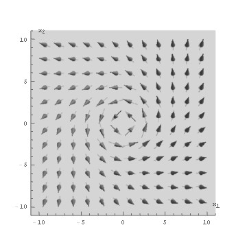
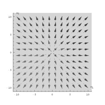
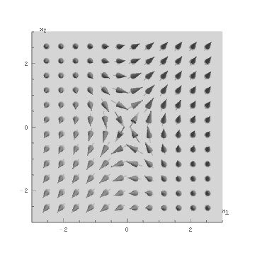
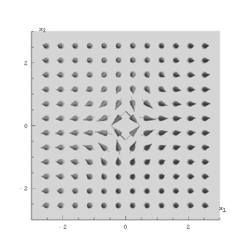
Figure 1: Top from left to right: Bloch skyrmion $v=-\frac{i}{2}\bar{z}$ in the theory with $\alpha=0$ and Néel skyrmion $v=\frac{1}{2}\bar{z}$ in the theory with $\alpha=\frac{\pi}{2}$. Bottom: anti-skyrmions in the theory with $\alpha=0$, with $v=-\frac{i}{2}\left(\bar{z}+4z\right)$ shown on the left and $v=-\frac{i}{2}\left(\bar{z}+6iz\right)$ on the right. Note that the magnetisation of anti-skyrmions rotates oppositely to that of the skyrmions when one traverses a positively oriented circle around the centre, where $v=0$ or $\boldsymbol{n}=(0,0,-1)^{t}$. Note also the different scale of the anti-skyrmion plots. Size and orientation of anti-skyrmions can be adjusted via the coefficient of $z$.

To sum up, as $|a|$ increases from zero we deform a hedgehog skyrmion through a line defect into an anti-skyrmion. In this process, the axisymmetric energy distribution of a hedgehog skyrmion is first squeezed and stretched into an elliptical shape and then into a line at $|a|=1$. As $|a|$ is increased further the energy distribution contracts again into an elliptical shape and shrinks; it never recovers the axisymmetry of the original skyrmion. In Fig. 1 we illustrate our discussion by showing the magnetisation of the basic Bloch and Néel skyrmions in our model, and also the magnetisation of two anti-skyrmions in the theory with $\alpha=0$.

Next we turn our attention to the family of solutions (4.55) with $N=2$. We have not fully explored the eight parameters in this family, of which three can again be accounted for by the symmetry operations of translation and rotation. Here, we only exhibit two interesting phenomena and fix $\alpha=0$ for definiteness. The first is the nonlinear superposition of skyrmions and anti-skyrmions in this model. Configurations of the form

$$v=-\frac{i}{2}\left(\bar{z}-\frac{z^{n}}{R^{n-1}}\right),\qquad R\in\mathbb{R}^{>0},\quad n\in\mathbb{Z}^{>1},$$ (5.4)

have degree $n$, but the functions $v$ have $(n+2)$ zeros: one at the origin and $(n+1)$ zeros at

$$z_{k}=Re^{\frac{2\pi ki}{n+1}},\quad k=0,\ldots,n.$$ (5.5)

The magnetisation takes the value $\boldsymbol{n}=(0,0,-1)^{t}$ at the zeros, but inspection of the winding shows that the configuration consists of a skyrmion at the origin surrounded by $(n+1)$ anti-skyrmions at the locations (5.5). The energy density (4.34) is peaked at the anti-skyrmion locations. Such superpositions of solitons and anti-solitons do not solve the Bogomol’nyi equations of the pure $O(3)$ sigma model, which require maps to be either holomorphic or antiholomorphic. In our model they are possible, essentially because the number of zeros for functions of the form (4.30) can exceed the absolute value of the degree. In fact, determining the number of zeros of (4.30) (and hence the number of skyrmions and anti-skyrmions counted without sign) is an interesting mathematical problem, see [21] for rigorous bounds and also [22, 23] for further results and the application of this problem to gravitational lensing.

Continuing with $\alpha=0$, we observe that rational solutions of the form

$$v=-\frac{i}{2}\left(\bar{z}-\frac{R^{2}}{z}\right),\quad R\in\mathbb{R}^{>0},$$ (5.6)

look like skyrmion bags [11] or sacks [12]. These particular bags have degree $Q=0$, take the vacuum value $\boldsymbol{n}=(0,0,1)^{t}$ at the origin and the value $\boldsymbol{n}=(0,0,-1)^{t}$ on a circle of radius $R$ centred at the origin. The energy density (4.34) is maximal on this circle. The solutions (5.6) are axisymmetric and an example of what is sometimes called skyrmionium in the literature. Clearly one can obtain more general bags by acting with translations on (5.6). We note that the circles of zeros of functions like (5.6) also play a special role in the context of gravitational lensing, where they are called Einstein rings [23].

6 Conclusion

In this paper we introduced models for magnetic skyrmions in the plane for which an infinite family of analytical solutions can be given explicitly. In our study we concentrated on the family of magnetic skyrmions determined by a rational holomorphic function according to (4.30). We showed that, with a suitable regularisation in the case of linear growth in the holomorphic function at infinity, the total energy takes the quantised values $4\pi N$, where $N$ is a positive integer which combines the degree with the (possibly regularised) total vorticity of a configuration. This integer does not appear to have been studied in the literature on magnetic skyrmions, but our study suggests that it plays an important role.

We also determined the collective coordinates or moduli of the solutions for given $N$, and studied example configurations for low values of $N$. They include remarkable deformations of Bloch and Néel skyrmions into line defects and anti-skyrmions. Finally, we exhibited some of the bag and multi-anti-skyrmion configurations included in the family (4.30).

Magnetic skyrmions are sometimes also called chiral skyrmions because the DM interaction breaks reflection symmetry. This is evident in our solutions through the mandatory and fixed anti-holomorphic part (of negative degree) but the optional holomorphic part (of positive degree). It is interesting and somewhat unexpected that our models allows for nonlinear superpositions of skyrmions and anti-skyrmions in static configurations. However, their roles are not symmetric. To obtain perfect mirrors of our models one would need to replace the DM interaction with the one of opposite chirality (2.11). One checks that this would lead to a Bogomol’nyi equation which enforces a fixed holomorphic part, but allows for an arbitrary anti-holomorphic part. This is consistent with the criterion derived in [16] for the preference of skyrmions over anti-skyrmions depending on the chirality.

The explicit family of solutions in our models and their chiral twins should be studied further in order to obtain a systematic understanding of the types of defects they capture. One would also like to understand how these defects relate to those observed in the various phases of generic models for magnetic skyrmions as discussed for example in [8].

Mathematically, one would like to understand more precisely the class of maps from the plane to the sphere for which the integrals defining the degree, total energy and total vortex strength are well-defined. It would also be important to ascertain if the energy functional (2.7) is bounded below for a suitably defined class of configurations (not just our solutions). In [19] it was shown that in a closely related model with a pure Zeeman potential the total energy is bounded below by a multiple of the absolute value of the degree. In our model, the energy is potentially unbounded below unless one imposes suitable behaviour at spatial infinity.

The second order variational equation (2.19) and the Bogomol’nyi equation (4.13) deserve further study. One would like to know, for example, if there are other finite-energy solutions (possibly after suitable regularisation) of the variational equation, not included in our rational family (4.30).

Finally, future work should include the study of time evolution and the effect of external fields on the solutions in our model.

Acknowledgements   B B-S and CR acknowledge EPSRC-funded PhD studentships. BJS thanks Christof Melcher for correspondence and for pointing out reference [17], and Paul Sutcliffe for helpful comments regarding the total energy of line defects in our model.

Note added   While this paper was under review, research was reported in the literature which has implications for the definition of energy in our models. A modification of the energy expression for magnetic skyrmions by a boundary term already proposed for analytical reasons in [19] was generalised in [24] in the framework of gauged sigma models. Applied to the models discussed here, this modification amounts to subtracting the total vorticity $\Omega_{\mathbb{R}^{2}}$ (2.1) from our energy (2.7) or, equivalently, to replacing $\boldsymbol{n}\cdot\nabla_{-\alpha}\times\boldsymbol{n}$ by $(\boldsymbol{n}-\boldsymbol{e}_{3})\cdot\nabla_{-\alpha}\times\boldsymbol{n}$ in (2.7). The modification does not affect the variational equations or the Bogomol’nyi equations studied here. The modified energy has the advantage of being finite without regularisation for all rational solutions of the form (4.30). In fact, for any such solution the modified energy is equal to $4\pi Q$, where $Q$ is the degree, instead of the value $4\pi N$ for our energy (after regularisation if required). On the other hand, the geometrical investigation reported in [25] shows that the integer $N$ (4.53) can be interpreted as the equivariant degree of the rational solutions (4.30), suggesting that the energy we used here is geometrically natural. It thus appears that there is a certain tension between the energy expressions preferred from an analytical and a geometrical point of view. Further work is required to resolve this.

References

- [1] A. N. Bogdanov and D. A. Yablonskii, Thermodynamically Stable ‘Vortices’ in Magnetically Ordered Crystals. The Mixed State of Magnets, Zh. Eksp. Teor. Fiz. 95 (1989) 178–182.
- [2] N. Nagaosa and Y. Tokura, Topological Properties and Dynamics of Magnetic Skyrmions, Nature Nanotechnology 8 (2013 ) 899–911, doi:10.1038/NNANO.2013.243.
- [3] I. Dzyaloshinskii, A Thermodynamic Theory of ‘Weak’ Ferromagnetism of Antiferromagnetics, J. Phys. Chem. Solids 4 (1958) 241–255, doi:10.1016/0022-3697(58)90076-3.
- [4] T. Moriya, Anisotropic Superexchange Interaction and Weak Ferromagnetism, Phys. Rev. 120 (1960) 91–98, doi:10.1103/PhysRev.120.91.
- [5] N. S. Manton and P. M. Sutcliffe, Topological Solitons, Cambridge Monographs on Mathematical Physics, Cambridge University Press, Cambridge, 2004, doi:10.1017/CBO9780511617034.
- [6] U. K. Rößler, A. N. Bogdanov and C. Pfleiderer, Spontaneous Skyrmion Ground States in Magnetic Metals, Nature 442 (2006) 797–801, doi:10.1038/nature05056.
- [7] X. Z. Yu, Y. Onose, N. Kanazawa, J. H. Park, J. H. Han, Y. Matsui, N. Nagaosa and Y. Tokura, Real-Space Observation of a Two-dimensional Skyrmion Crystal, Nature 465 (2010) 901–904, doi:10.1038/nature09124.
- [8] M. N. Wilson, A. B. Butenko, A N. Bogdanov and T. L. Monchesky, Chiral Skyrmions in Cubic Helimagnet Films: The Role of Uniaxial Anisotropy, Phys. Rev. B 89 (2014) 094411, doi:10.1103/PhysRevB.89.094411.
- [9] A. Bogdanov and A Hubert, Thermodynamically Stable Magnetic Vortex States in Magnetic Crystals, J. Magn. Magn. Mater. 138 (1994) 255–269,doi:10.1016/0304-8853(94)90046-9.
- [10] A. O. Leonov and I. Kézsmárki, Asymmetric Isolated Skyrmions in Polar Magnets with Easy-plane Anisotropy, Phys. Rev. B 96 (2017) 014423,doi:10.1103/PhysRevB.96.014423.
- [11] D. Foster, C. Kind, P. J. Ackerman, J. S. B. Tai, M. R. Dennis and I. I. Smalyukh, Two-dimensional Skyrmion Bags in Liquid Crystals and Ferromagnets, Nature Physics 15, 655 (2019), doi:10.1038/s41567-019-0476-x.
- [12] F. N. Rybakov and N. S. Kiselev, Chiral Magnetic Skyrmions with Arbitrary Topological Charge (‘Skyrmionic Sacks’), Phys. Rev. B 99, 064437 (2019), doi:10.1103/PhysRevB.99.064437.
- [13] A. A. Belavin and A. M. Polyakov, Metastable States of Two-dimensional Isotropic Ferromagnets, JETP Lett. 22 (1975) 245.
- [14] B. M. A. G. Piette, B. J. Schroers and W. J. Zakrzewski Multisolitons in a 2-dimensional Skyrme Model, Zeitschrift für Physik C 65 (1995) 165–174, doi:10.1007/BF01571317.
- [15] B. J. Schroers, Bogomol’nyi Solitons in a Gauged O(3) Sigma Model, Phys. Lett. B 356 (1995) 291–296, doi:10.1016/0370-2693(95)00833-7.
- [16] M. Hoffmann, B. Zimmermann, G. P. Müller, D. Schürhoff, N. S. Kiselev, C. Melcher and S. Blügel, Antiskyrmions Stabilized at Interfaces by Anisotropic Dzyaloshinskii-Moriya Interactions, Nature Communications 8 (2017) 308, doi:10.1038/s41467-017-00313-0.
- [17] L. Döring and C. Melcher, Compactness Results for Static and Dynamic Chiral Skyrmions near the Conformal Limit, Calc. Var. (2017) 56:60, doi:10.1007/s00526-017-1172-2.
- [18] G. Nardelli, Magnetic Vortices from a Nonlinear Sigma Model with Local Symmetry, Phys. Rev. Lett. 73 (1994) 2524–2527, doi:10.1103/PhysRevLett.73.2524.
- [19] C. Melcher, Chiral Skyrmions in the Plane, Proc. R. Soc. A 470 (2014) 20140394, doi:10.1098/rspa.2014.0394.
- [20] G. ’t Hooft, Magnetic Monopoles in Unified Gauge Theories, Nucl. Phys. B79 (1974) 276–284, doi:10.1016/0550-3213(74)90486-6.
- [21] D. Khavinson and G. Neumann, On the Number of Zeros of Certain Rational Harmonic Functions, Proc. Amer. Math. Soc. 134 (2005) 1077–1085, doi:10.1090/S0002-9939-05-08058-5.
- [22] P. M. Bleher, Y. Homma, L. L. Ji, R. K. W. Roeder, Counting Zeros of Harmonic Rational Functions and its Application to Gravitational Lensing, International Mathematics Research Notices, Volume 2014 (2014), 2245–2264, doi:10.1093/imrn/rns284.
- [23] C. Fassnacht, C. Keeton and D. Khavinson, Gravitational Lensing by Elliptical Galaxies, and the Schwarz Function. In: Gustafsson B., Vasil’ev A. (eds) Analysis and Mathematical Physics. Trends in Mathematics. Birkhäuser Basel, 2009, doi:10.1007/978-3-7643-9906-1_6.
- [24] B. J. Schroers, Gauged Sigma Models and Magnetic Skyrmions, SciPost Phys. 7 (2019) 030, doi:10.21468/SciPostPhys.7.3.030.
- [25] E. Walton, Some Exact Skyrmion Solutions on Curved Thin Films, https://arxiv.org/abs/1908.08428.