Worst-case Bounds and Optimized Cache on $M^{th}$ Request Cache Insertion Policies under Elastic Conditions

Abstract.

Cloud services and other shared third-party infrastructures allow individual content providers to easily scale their services based on current resource demands. In this paper, we consider an individual content provider that wants to minimize its delivery costs under the assumptions that the storage and bandwidth resources it requires are elastic, the content provider only pays for the resources that it consumes, and costs are proportional to the resource usage. Within this context, we (i) derive worst-case bounds for the optimal cost and competitive cost ratios of different classes of cache on $M^{th}$ request cache insertion policies, (ii) derive explicit average cost expressions and bounds under arbitrary inter-request distributions, (iii) derive explicit average cost expressions and bounds for short-tailed (deterministic, Erlang, and exponential) and heavy-tailed (Pareto) inter-request distributions, and (iv) present numeric and trace-based evaluations that reveal insights into the relative cost performance of the policies. Our results show that a window-based cache on $2^{nd}$ request policy using a single threshold optimized to minimize worst-case costs provides good average performance across the different distributions and the full parameter ranges of each considered distribution, making it an attractive choice for a wide range of practical conditions where request rates of individual file objects typically are not known and can change quickly.

1. Introduction

Cloud services and other shared infrastructures are becoming increasingly common. These infrastructures are typically third-party operated and allow individual service providers using them to easily scale their services based on current resource demands. In the context of content delivery, rather than buying and operating their own dedicated servers, many content providers are already using third-party operated Content Distribution Networks (CDNs) and cloud-based content delivery platforms. This trend towards using third-party providers on an on-demand basis is expected to increase as new content providers enter the market.

Motivated by current on-demand cloud-pricing models, in this paper, we consider an individual content provider that wants to minimize its delivery costs under the assumptions that the resources it requires to deliver its service are elastic, the content provider only pays for the resources it consumes, and costs are proportional to the resource usage. For the purpose of our analysis, we consider a simple cost model in which the content provider pays the third-party service for (i) the amount of storage it consumes due to caching close to the end-users and (ii) the amount of (backhaul) bandwidth that it and its end-users consume. Under this model, we then analyze the optimized delivery costs of different cache on $M^{th}$ request cache insertion policies when using a Time-to-Live (TTL) based eviction policy in which a file object remains in the cache after insertion until a time interval $T$ has elapsed without any requests for the object.

It is important to note that although use of a TTL eviction policy has been shown useful in approximating the performance of a fixed-size Least-Recently-Used (LRU) cache when the number of file objects is sufficiently large (Che et al., 2002; Fricker et al., 2012; Bianchi et al., 2013; Berger et al., 2014; Garetto et al., 2016; Carlsson and Eager, 2018), and our results may therefore provide some insight for this case, it is not the focus of this paper. Here we assume elastic resources, where cache eviction is not needed to make space for a new insertion, but rather to reduce cost by removing objects that are not expected to be requested again soon. A TTL-based eviction policy is a good heuristic for such purposes. Cloud service providers already provide elastic provisioning at varying granularities for computation and storage, and in the context of trends such as serverless computing, in-memory caching, and multi-access edge computing, we believe that support for fine-grained elasticity may increase in the future.

In the past, selective cache insertion policies have been shown valuable in reducing cache pollution due to ephemeral content popularity and the long tail of one-timers observed in edge networks (Gill et al., 2007; Zink et al., 2009; Maggs and Sitaraman, 2015; Carlsson and Eager, 2017). However, prior work has not bounded or optimized the worst-case delivery costs of such policies.

In this paper, we first present novel worst-case bounds for the optimal cost and competitive cost-ratios of different variations of these policies. Second, we derive explicit average cost expressions and cost ratio bounds for these policies under arbitrary inter-request time distributions, assuming independent and identically distributed request times, as well as for specific short-tailed (deterministic, Erlang, and exponential) and heavy-tailed (Pareto) inter-request time distributions. Our analysis includes comparisons against both optimal offline policy bounds and, for the case when hazard rates are increasing or constant, optimal online policy bounds; all derived here. Finally, we present numeric and trace-based evaluations and provide insights into the relative cost performance of the policies.

Our analysis reveals that window-based cache on $M^{th}$ request cache insertion policies can substantially outperform policies that do not take into account the recency of prior object requests when making cache insertion decisions. With window-based cache on $M^{th}$ request policies a counter is maintained for each uncached object that has been requested at least once within the last $W$ time units. A newly allocated counter is initialized to one, and the counter is incremented by one whenever the object is referenced within $W$ time units of its most recent previous request. The object is inserted into the cache whenever the counter reaches $M$. Our results show that a single parameter version of this policy can be used beneficially, in which $W=T$, and that the best worst-case bounds are achieved by selecting the window size $W=T$ equal to the time that it takes to accumulate a cache storage cost (for that object) equal to the remote bandwidth cost $R$ associated with a cache miss (for that object). With these protocol settings, the worst-case bounds of the window-based cache on $M^{th}$ request policies have a competitive ratio of $M+1$ (compared to the optimal offline policy). While these ratios at first may appear discouraging for larger $M$, our average case analysis for different inter-request time distributions clearly shows substantial cost benefits of using intermediate $M$ such as 2-4, with the best choice depending on where in the parameter region the system operates. For less popular objects a slightly larger $M$ (e.g., $M=4$) may be beneficial; however, in general, window-based cache on $M^{th}$ request with $M=2$ typically provides the most consistently good average performance across the full parameter ranges of each considered distribution. Overall, the results show that using this policy with optimal worst-case parameter setting (i.e., $W=T=R$) may be attractive for practical conditions, where request rates of individual objects typically are not known and can change quickly.

The remainder of the paper is organized as follows. Sections 2 and 3 present our system model and the practical insertion policies considered, respectively. Section 4 presents the optimal offline policy and derives worst-case bounds for the different insertion policies. Section 5 presents cost expressions for the optimal offline bound under both arbitrary and specific distributions. Section 6 presents the corresponding expressions for an optimized baseline policy that assumes knowledge of the precise inter-request time distribution for each object, and shows that this policy has the same performance as the optimal online policy when hazard rates are increasing or constant. Section 7 then derives general cost expressions for the practical insertion policies, before Section 8 presents the distribution-specific expressions, analyzes the relative performance of the policies, and compares their costs against the offline optimal and optimized baselines. Section 9 complements the single-file analysis results with both analytic and trace-based multi-file evaluations. Finally, Section 10 discusses related work and Section 11 presents our conclusions.

2. System Model

Initially, let us consider the costs associated with a single file object as seen at a single cache location. (The multi-file case is considered in Section 9.) Furthermore, without loss of generality, for this object and location, let us assume that the provider pays (i) a (normalized) storage cost of $1$ per time unit that the file object is stored in the cache and (ii) a remote bandwidth cost $R$ each time a request is made to an object currently not in cache. At these times, the file object needs to be retrieved from the origin servers (or a different cache), which results in additional bandwidth costs (and delivery delays). Note that $R$ is defined as the incremental delivery cost, beyond that of delivering the content from the cache to the client. This latter (typically much smaller) baseline delivery cost is therefore policy independent and always incurred. We obtain worst-case bounds on cost ratios by assuming it to be zero. Setting it to zero also allows us to entirely focus on the policy dependent costs. Finally, note that a third party service’s accounting for storage and remote bandwidth costs would, in practice, be based on particular time, size, and bandwidth granularities. The finer-grained the accounting, the more closely our model would correspond to the real system.

At the time a request is made for a file object not currently in the cache, the system must, in an online fashion, decide whether the object should be cached or not. Naturally, the total delivery cost of different caching policies will depend substantially on the choices made and the request patterns of consideration.

To illustrate the impact of these choices, consider the most basic TTL-based cache policy that inserts a file object into the cache whenever a request is made for the object (and the object is not currently in the cache) and retains the object until $T$ time units elapse with no requests. This policy would incur a total cost of $R+T$ if a single request is made for the object. However, if it was known that the object would only receive a single request, it would be optimal to not cache the object at all. In this case, it is easy to see that the minimal delivery cost is $R$. For this particular example, the cost ratio between the basic TTL-based policy and the (offline) optimal is therefore $\frac{R+T}{R}$. In general, we want these cost ratios to be as small as possible both for (i) worst-case request patterns where an adversary selects the request pattern and (ii) average case scenarios with more realistic request patterns. Section 4 and Sections 5-7 provide worst-case and average-case analysis, respectively, for different TTL-based cache on $M^{th}$ request insertion policies (Section 3).

3. Insertion policies

In this paper, we compare the delivery costs of different cache on $M^{th}$ request insertion policies when using a TTL-based eviction policy in which an object remains in the cache after insertion until a time interval $T$ has elapsed without any requests for the object. Note that with elastic resources, eviction is not needed for making room for new objects, but instead is needed for reduction of storage costs. As we show, a simple TTL rule is very effective for this purpose. We next describe the insertion policies considered in this paper.

• Always on $1^{st}$ ($T$): Always cache a requested object if not in the cache already and keep it in the cache until $T$ time units have passed since the most recent request.

• Always on $M^{th}$ ($M,T$): The system maintains a counter for how many times each uncached object has been requested. When the counter reaches $M$ the object is cached, and is kept in the cache until $T$ time units have passed since the most recent request, at which point the object is evicted and the counter is reset to 0. For $M=1$, this corresponds to always on $1^{st}$.

• Single-window on $M^{th}$ ($M,T$): The system maintains a counter for each uncached object that has been requested at least once within the last $T$ time units. The respective counter is initialized to one the first time that a request is made to an object or when a request is made to an object that has not been requested within the last $T$ time units. The counter is incremented by one whenever the object is referenced within $T$ time units of its most recent previous request. Finally, when the counter reaches $M$, the object is cached. Again, the object remains in the cache until a time interval $T$ has elapsed without any requests for the object. For $M$=$1$, this policy corresponds to always on $1^{st}$.

• Dual-window on $2^{nd}$ ($W,T$): This policy is similar to single-window on 2^nd, but uses a potentially tighter time threshold $W\leq T$ for determining when to add an object to the cache. With the dual-window on $2^{nd}$ policy, when an uncached object is requested it is added to the cache if there has been a previous request for the object within the last $W$ time units, and is kept in the cache until $T$ time units have passed since the most recent request. This policy reduces to the basic single-window on $2^{nd}$ when $W=T$.

4. Worst case bounds

For this analysis we consider an arbitrary request sequence $\mathcal{A}=\{a_{i}\}$ for a single object with $N$ requests, where $a_{i}$ is the inter-request time between requests $i$ and $i-1$ ($2\leq i\leq N$). We assume that the object is initially uncached.

4.1. Offline optimal lower bound

We first derive the cost expression for the optimal (offline) caching policy (across all possible policy classes; not restricted to TTL-based policies) for the case when the cache has perfect prior knowledge of the request sequence $\mathcal{A}$. The first request will always incur a remote bandwidth cost $R$. For each of the later requests $i$ ($2\leq i\leq N$), in the (offline) optimal case, the object should have been cached (if not already in the cache) at the time of the $(i-1)^{st}$ request and remain retained until at least the $i^{th}$ request, whenever $a_{i}<R$. On the other hand, if $a_{i}>R$, the object should not have been cached at the time of the $i-1^{st}$ request, or should have been dropped from the cache (if it was already in the cache) just after serving request $i-1$. In this case, the $i^{th}$ request should incur the remote bandwidth cost $R$. The following lemma regarding the (offline) optimal cost follows directly from these observations.

Lemma 4.1.

Given an arbitrary request sequence $\mathcal{A}$, the minimum total delivery cost of the optimal offline policy is:

(1) $$C_{opt}^{offline}=R+\sum_{i=2}^{N}\min[a_{i},R].$$

Lemma 4.1 provides a fundamental offline bound for all caching policies. We next derive worst-case bounds for the various online policies outlined in Section 3.

4.2. Always on $1^{st}$ ($T$)

For an arbitrary request sequence $\mathcal{A}$, this (online) policy incurs a total delivery cost equal to:

(2) $$C^{always}_{M=1,T}=R+T+\sum_{i=2}^{N}x_{i},$$

where

(5) $$x_{i}=\left\{\begin{array}[]{ll}T+R,&\textrm{if}~{}a_{i}>T\\ a_{i},&\textrm{otherwise}.\\ \end{array}\right.$$

Here, and throughout the paper, we use the superscript on the cost $C$ to indicate the class of insertion policy, the subscript to indicate the parameters being used by the policy, and potential parameter assignment to indicate potential special cases considered. In equation (2), the $R$ term corresponds to the cost of retrieving a copy of the object to serve the first request in the sequence and the $T$ term corresponds to the cache storage cost incurred after the last request. For requests $2\leq i\leq N$, equation (5) then takes into account whether request $i$ occurs within $T$ of the prior request (implying an additional storage cost of $a_{i}$) or the object has been removed from the cache prior to the request (implying an additional storage cost $T$ before the object was evicted and a bandwidth cost $R$ to retrieve a new copy). Given equations (1)-(5), it is now possible to show the following theorem.

Theorem 4.2.

The best (optimal) competitive ratio using always on $1^{st}$ is achieved with $T=R$ and is equal to 2. More specifically,

(6) $$\max_{\mathcal{A}}\frac{C^{always}_{M=1,T=R}}{C_{opt}^{offline}}\leq\max_{\mathcal{A}}\frac{C^{always}_{M=1,T}}{C_{opt}^{offline}}$$

for all $T$, and $\frac{C^{always}_{M=1,T=R}}{C_{opt}^{offline}}\leq 2$ for all possible sequences $\mathcal{A}=\{a_{i}\}$.

Proof.

We consider an arbitrary request sequence $\mathcal{A}$ with $N$ requests and then bound the cost ratio based on the worst-case patterns that an adversary could create. For this and the following proofs we note that the first request always must incur a remote bandwidth cost $R$ and then focus on the worst-case pattern of the remaining $N-1$ requests.

Case $T\leq R$: For the remaining $N-1$ requests, let us define the following sets: $S=\{i|a_{i}\leq T\}$, $S^{\prime}=\{i|T<a_{i}\leq R\}$, and $S^{\prime\prime}=\{i|R<a_{i}\}$. Note that the set $S$ consists of those requests that would result in cache hits, if using always on $1^{st}$, while the requests in the other sets would result in cache misses. Also, note that the requests in both set $S$ and $S^{\prime}$ would result in the optimal offline policy retrieving the object from the local cache. Now, for any request sequence $\mathcal{A}$, we have the following relations:

$$\frac{C^{always}_{M=1,T}}{C_{opt}^{offline}} =\frac{R+\sum_{i\in S}a_{i}+(|S^{\prime}|+|S^{\prime\prime}|)(T+R)+T}{R+\sum_{i\in S}a_{i}+\sum_{i\in S^{\prime}}a_{i}+|S^{\prime\prime}|R}$$

$$\leq\frac{(R+T)(1+|S^{\prime\prime}|)+(R+T)|S^{\prime}|}{R(1+|S^{\prime\prime}|)+\sum_{i\in S^{\prime}}a_{i}}$$

(7) $$\leq\frac{(R+T)(1+|S^{\prime\prime}|)+(R+T)|S^{\prime}|}{R(1+|S^{\prime\prime}|)+|S^{\prime}|T}\leq\frac{R+T}{T}.$$

To establish the three inequalities in (4.2) we have used that: (i) $\frac{X+\sum_{i\in S}a_{i}}{X(1-\epsilon)+\sum_{i\in S}a_{i}}\leq\frac{X}{X(1-\epsilon)}$ for $0\leq\epsilon\leq 1$ and $\sum_{i\in S}a_{i}\geq 0$, (ii) $T\leq a_{i}$ when $i\in S^{\prime}$, and (iii) $\frac{d}{dx}(\frac{R+T}{R(1-x)+xT})=-\frac{(R+T)(T-R)}{(R+x(T-R))^{2}}\geq 0$ when $T\leq R$, respectively. Clearly, since $\frac{R+T}{T}$ is monotonically decreasing for the range $0\leq T\leq R$, the (above) worst-case bound is tightest when $T\rightarrow R$ (equal to 2).

Case $R\leq T$: Let us define the following sets for $2\leq i\leq N$: $G=\{i|a_{i}<R\}$, $G^{\prime}=\{i|R\leq a_{i}\leq T\}$, and $G^{\prime\prime}=\{i|T<a_{i}\}$. Here, sets $G$ and $G^{\prime}$ consist of those requests that would result in cache hits with always on $1^{st}$, but only the requests in set $G$ would result in cache hits with the optimal offline policy. Using a similar approach as for the first case, we obtain the following:

$$\frac{C^{always}_{M=1,T}}{C_{opt}^{offline}} =\frac{R+\sum_{i\in G}a_{i}+\sum_{i\in G^{\prime}}a_{i}+|G^{\prime\prime}|(T+R)+T}{R+\sum_{i\in G}a_{i}+(|G^{\prime}|+|G^{\prime\prime}|)R}$$

$$\leq\frac{(R+T)(1+|G^{\prime\prime}|)+\sum_{i\in G^{\prime}}a_{i}}{R(1+|G^{\prime\prime}|)+|G^{\prime}|R}$$

(8) $$\leq\frac{(R+T)(1+|G^{\prime\prime}|)+T|G^{\prime}|}{R(1+|G^{\prime\prime}|)+|G^{\prime}|R}\leq\frac{R+T}{R}.$$

Here, the first inequality is derived in the same way as the first inequality in (4.2), the second inequality uses the fact that $a_{i}\leq T$ when $i\in G^{\prime}$, and the third inequality uses the fact that $\frac{d}{dx}(\frac{(R+T)(1-x)+Tx}{R})=-1<0$. Now, since $\frac{R+T}{R}$ has its minimum in the range $R\leq T$ when $T=R$, we have that $T=R$ provides the tightest bound (equal to 2).

Finally, inserting $T=R$ into either of the two bounds, we obtain the worst-case bound of 2. The bound is tight and is achieved, for example, when requests are evenly spaced by $T+\epsilon$, for some $\epsilon>0$. In this case, $|S|=|G|=|G^{\prime}|=0$ and $\frac{C^{awlays}_{M=1,T=R}}{C_{opt}^{offline}}=\frac{T+R}{R}=2$. ∎

4.3. Always on $M^{th}$ ($M,T$)

By generalizing the techniques used to prove the worst-case properties of always on $1^{st}$ to consider additional counter states, it is possible to prove the following theorem.

Theorem 4.3.

The best (optimal) competitive ratio using the always on $M^{th}$ policy is achieved with $T=R$ and is equal to $M+1$. More specifically,

(9) $$\max_{\mathcal{A}}\frac{C^{always}_{M,T=R}}{C_{opt}^{offline}}\leq\max_{\mathcal{A}}\frac{C^{always}_{M,T}}{C_{opt}^{offline}}$$

for all $T$, and $\frac{C^{always}_{M,T=R}}{C_{opt}^{offline}}\leq M+1$ for all possible sequences $\mathcal{A}=\{a_{i}\}$.

A proof for Theorem 4.3 is provided in the Appendix. Similar to the proof for always on $1^{st}$, the proof identifies sets of inter-request times $a_{i}$ based on differences and similarities in how the always on $M^{th}$ policy and the optimal offline policy treat these sets of requests. In particular, sets are defined based on the states of the always on $M^{th}$ policy (depending on the object’s caching status and, if uncached, counter value) and how $a_{i}$ relates to $T$ and $R$. This generalizes the number of (mutually exclusive) sets of requests from $2\times 3$ for the always on $1^{st}$ policy, to $2\times(2M+1)$ for the general always on $M^{th}$ policy, where $2M+1$ sets are needed for each of the two cases when $T\leq R$ and $R\leq T$, respectively.

Using this proof method, we also identify a request pattern that shows that the bound is tight. In particular, the worst-case bound is achievable by a request pattern in which requests occurs in batches of $M$ requests, and the batches are separated by more than $\max[R,T]$ time units. To see this, let us consider the $T\leq R$ case. In this case, with the above request sequence, in each batch cycle, the always on $M^{th}$ policy downloads the object $M$ times, finally stores a copy at the time of the $M^{th}$ request, and then keeps it in the cache for $R$ time units. This pattern results in a total cost of $(M+1)R$ per batch. In contrast, the optimal offline policy downloads a single copy (at cost $R$), serves all $M$ requests using this copy, and then immediately deletes the copy, incurring negligible storage costs. The argument for the $R\leq T$ case is analogous.

4.4. Single-window on $M^{th}$ ($M,T$)

While the number of counter states to consider is the same for single-window on $M^{th}$ as for always on $M^{th}$, the possible state transitions when the counter is below $M$ differ (e.g., counter is reset each time there is no request within a window $T$). To account for this, our proof of the following theorem for the single-window on $M^{th}$ policy requires $2\times(M-1)$ additional sets to be defined ($M-1$ for when $T\leq R$ and $M-1$ for when $R\leq T$).

Theorem 4.4.

The best (optimal) competitive ratio using the single-window on $M^{th}$ policy is achieved with $T=R$ and is equal to $M+1$. More specifically,

(10) $$\max_{\mathcal{A}}\frac{C^{window}_{M,T=R}}{C_{opt}^{offline}}\leq\max_{\mathcal{A}}\frac{C^{window}_{M,T}}{C_{opt}^{offline}}$$

for all $T$, and $\frac{C^{window}_{M,T=R}}{C_{opt}^{offline}}\leq M+1$ for all possible sequences $\mathcal{A}=\{a_{i}\}$.

A proof for Theorem 4.4 is provided in the Appendix. Interestingly, the same request pattern, with batches of size $M$ separated by at least $\max[T,R]$, as used to show that Theorem 4.3 is tight, provides proof that Theorem 4.4 is tight.

4.5. Dual-window on $2^{nd}$ ($W,T$)

Using similar methods as used in prior subsections (this time based on $3\times 8$ sets, accounting for the relationship of $a_{i}$ to $W$, $T$ and $R$), it is possible to prove the following theorem establishing that dual-window on $2^{nd}$ has the same worst-case properties as single-window on $2^{nd}$. A proof is provided in the Appendix.

Theorem 4.5.

The best (optimal) competitive ratio using the dual-window on $2^{nd}$ policy is achieved with $T=W=R$ and is equal to 3. More specifically,

(11) $$\max_{\mathcal{A}}\frac{C^{window}_{M=2,W=R,T=R}}{C_{opt}^{offline}}\leq\max_{\mathcal{A}}\frac{C^{window}_{M=2,W,T}}{C_{opt}^{offline}}$$

for all $W$ and $T$, and $\frac{C^{window}_{M=2,W=R,T=R}}{C_{opt}^{offline}}\leq 3$ for all possible request sequences $\mathcal{A}=\{a_{i}\}$.

5. Steady-state: Offline Bound

Thus far our results have not made any restrictions to the request sequences. For the remaining analysis in this paper, we assume that inter-request times are independent and identically distributed. Under this assumption, we derive expressions for a general inter-request time distribution $f(t)$ with cumulative distribution function $F(t)$, as well as for specific example distributions. In the following, we let $E[a_{i}]$ denote the average inter-request time, we let

(12) $$E[a_{i}|a_{i}\leq X] =\frac{\int_{0}^{X}tf(t)\textrm{dt}}{\int_{0}^{X}f(t)\textrm{dt}}=X-\frac{1}{F(X)}\int_{0}^{X}F(t)\textrm{dt}$$

denote the average inter-request time given that the inter-request time is no more than $X$ time units, and we let

(13) $$P(a\leq X|a>Y) =\frac{\int_{Y}^{X}f(t)\textrm{dt}}{\int_{Y}^{\infty}f(t)\textrm{dt}}=\frac{F(X)-F(Y)}{1-F(Y)}$$

denote the (conditional) probability that an inter-request time is no more than $X$ given that the inter-request time is greater than $Y$ time units. In this section we derive results for the optimal offline policy, while in Sections 6-8 we consider online policies.

5.1. General inter-request time distribution

Throughout this analysis we will derive expressions for the average cost per time unit. For the (optimal) offline policy, this cost can be calculated as the expected cost associated with an arbitrary request divided by the average inter-request time $E[a_{i}]$:

$$C_{opt}^{offline} =\frac{1}{E[a_{i}]}\left[\int_{0}^{R}tf(t)\textrm{dt}+R\int_{R}^{\infty}f(t)\textrm{dt}\right]$$

$$=\frac{1}{E[a_{i}]}\left[[tF(t)]_{0}^{R}-\int_{0}^{R}F(t)\textrm{dt}+R(1-F(R))\right]$$

(14) $$=\frac{1}{E[a_{i}]}\left[R-\int_{0}^{R}F(t)\textrm{dt}\right].$$

Here, we associate all requests with inter-request times $t$ less than $R$ with the cost $t$ to keep the object in the cache for an additional $t$ time units (first integral in the first line), while all other requests (with $R<t$) incur a cost $R$ (second integral in the first line). We then use integration by parts (step 2) and algebraic simplifications (step 3) to derive the final expression.

5.2. Example distributions

We next consider four example distributions.

Exponential: Assuming a Poisson process, with exponential inter-request times, we have

(15) $$f(t) =\lambda e^{-\lambda t},\quad F(t)=1-e^{-\lambda t},\quad E[a_{i}]=\frac{1}{\lambda}$$

(16) $$\int_{0}^{t}F(t)\textrm{dt} =t-\frac{1-e^{-\lambda t}}{\lambda}.$$

Through insertion of these equations into equation (5.1) we obtain the following cost function:

(17) $$C_{opt}^{offline} =\lambda\left[R-\frac{1-e^{-\lambda R}}{\lambda}\right]=1-e^{-\lambda R}.$$

Erlang: We next consider Erlang distributed inter-request times with shape parameter $k$ (integer) and rate parameter $\lambda>0$:

(18) $$f(t)=\frac{\lambda^{k}t^{k-1}e^{-\lambda t}}{(k-1)!},~{}F(t)=1-\sum_{n=0}^{k-1}\frac{1}{n!}e^{-\lambda t}(\lambda t)^{n},~{}E[a_{i}]=\frac{k}{\lambda},$$

(19) $$\int_{0}^{t}F(t)\textrm{dt}=t-\frac{k}{\lambda}+\frac{e^{-\lambda t}}{\lambda}\sum_{m=1}^{k}\sum_{n=0}^{m-1}\frac{(\lambda t)^{n}}{n!}.$$

Substitution into equation (5.1) yields:

(20) $$C_{opt}^{offline} =1-\frac{e^{-\lambda R}}{k}\sum_{m=1}^{k}\sum_{n=0}^{m-1}\frac{(\lambda R)^{n}}{n!}.$$

Deterministic: In the extreme case for low variability, all inter-request times are equal to a constant $a$. Let $\delta_{a}(t)$ and $u_{a}(t)$ represent the Dirac delta function and the unit step function, both with (unit) singularities at $t=a$. Then, we have:

(21) $$f(t) =\delta_{a}(t),\quad F(t)=u_{a}(t),\quad E[a_{i}]=a,$$

(22) $$\int_{0}^{t}F(t)\textrm{dt} =\max[0,t-a].$$

Substitution into equation (5.1) yields:

(23) $$C_{opt}^{offline} =\min[1,\frac{R}{a}].$$

Pareto: Finally, we consider Pareto distributed inter-request times (as an example of heavy-tailed distributions) with shape parameter $\alpha>1$ (when $0<\alpha\leq 1$ the expected inter-request time is infinite) and scale parameter $t_{m}>0$. In this case, we have:

(24) $$f(t) =\frac{\alpha t_{m}^{\alpha}}{t^{\alpha+1}},\quad F(t)=1-\left(\frac{t_{m}}{t}\right)^{\alpha},\quad t_{m}\leq t,$$

(25) $$\quad\quad E[a_{i}]=\frac{\alpha t_{m}}{\alpha-1},$$

(28) $$\int_{0}^{t}F(t)\textrm{dt} =\left\{\begin{array}[]{ll}t+\frac{t\left(\frac{t_{m}}{t}\right)^{\alpha}-t_{m}\alpha}{\alpha-1},&t_{m}\leq t\\ 0,&t<t_{m}.\\ \end{array}\right.$$

Substitution into equation (5.1) yields:

(31) $$C_{opt}^{offline} =\left\{\begin{array}[]{ll}1-\frac{1}{\alpha}\left(\frac{t_{m}}{R}\right)^{\alpha-1},&t_{m}\leq R\\ \frac{R(\alpha-1)}{\alpha t_{m}},&R<t_{m}.\\ \end{array}\right.$$

6. Steady-state: Static Baseline Policy with Known Inter-request Distribution

To provide some estimates for the best possible online cache performance, in this section we consider the case when an “oracle” provider knows the precise inter-request time distribution for each object. For this case, we consider a static baseline policy that tries to minimize the delivery cost by selecting between the extremes of (i) always keeping the object in the cache, or (ii) never caching the object.

6.1. Optimal online policy when non-decreasing hazard rate

Interestingly, the static baseline provides an online bound when the inter-request distribution parameters are known and the distribution has an increasing or constant hazard rate.

Theorem 6.1.

Static baseline achieves the minimum cost of any online policy when the inter-request distribution has an increasing or constant hazard rate.

Proof.

Since inter-request times are IID, we need consider only a single representative inter-request time between requests $i-1$ and $i$, for some $i\geq 2$. After servicing request $i-1$, any online policy will, at each subsequent instant of time up to the time of request $i$ or until the object is discarded, need to decide whether to retain the object in the cache, or evict it. The only information the online policy can use to make this decision is the elapsed time since request $i-1$. Therefore, any online policy will have a threshold parameter $t^{*}$, such that as long as the time since request $i-1$ is less than $t^{*}$, the object is retained. If time $t^{*}$ elapses before getting request $i$, the object is evicted. Letting $C(t^{*})$ denote the expected cost incurred from after servicing request $i-1$, up to and including the servicing of request $i$, we have:

(32) $$C(t^{*}) =F(t^{*})E[a_{i}|a_{i}\leq t^{*}]+(1-F(t^{*}))(R+t^{*}).$$

Using expression (12) and simplifying gives:

(33) $$C(t^{*}) =R(1-F(t^{*}))+t^{*}-\int_{0}^{t^{*}}F(t)\textrm{dt}.$$

Taking the derivative with respect to $t^{*}$ gives:

(34) $$\frac{dC(t^{*})}{dt^{*}} =1-F(t^{*})-Rf(t^{*}).$$

A constant hazard rate corresponds to an exponential distribution, and for this case it is straightforward to show that the derivative is negative for all $t^{*}$, positive for all $t^{*}$, or is constant at 0 for all $t^{*}$ (when $R\lambda=1$), implying that the static baseline policy achieves minimum cost. Consider now the case of increasing hazard rate, and note that the derivative is zero when $R=\frac{1-F(t^{*})}{f(t^{*})}$.

Whether such a point is a minimum or maximum depends on the second derivative, given by

(35) $$\frac{d^{2}C(t^{*})}{d^{2}t^{*}}=-f(t^{*})-R\frac{df(t^{*})}{dt^{*}}.$$

At a point where $R=\frac{1-F(t^{*})}{f(t^{*})}$, the second derivative is less than zero exactly when the derivative of the hazard rate at this point (the derivative of $f(t^{*})/(1-F(t^{*}))$) is positive. And so, when there is an increasing hazard rate, any point where $R=\frac{1-F(t^{*})}{f(t^{*})}$ is a local cost maximum, and the minimum cost must occur for $t^{*}=0$ or $t^{*}\rightarrow\infty$. ∎

Corollary 6.2.

For inter-request time distributions such that (i) there is a unique value of $t^{*}$ where $R=(1-F(t^{*}))/f(t^{*})$, and (ii) the derivative of the hazard rate at this value is negative, the minimum cost over all online policies is achieved with $t^{*}$ set to this value.

Note that the cache on $M^{th}$ policies are identical to the static baseline if $T$ (and $W$ in the case of dual-window) are chosen to be either 0 or $\infty$, whichever gives the best performance. Therefore, since static baseline provides an online bound when the inter-request distribution parameters are known and the distribution has an increasing or constant hazard rate, also the cache on $M^{th}$ policies with optimized parameters achieve this bound in this case.

In contrast to the case of the short-tailed distributions (deterministic, Erlang, and exponential), for which static baseline is the optimal online policy, with Pareto (and other heavy-tailed distributions) the competitive ratio of static baseline is unbounded (see Theorem 6.6 for the case of the Pareto distribution) even when request rates are known. For a Pareto distribution, using (24) to substitute for $F(t^{*})$ and $f(t^{*})$ in $R=(1-F(t^{*}))/f(t^{*})$ yields $t^{*}=R\alpha$, under the condition that $t^{*}=R\alpha\geq t_{m}$. Since Pareto has decreasing hazard rate for $t\geq t_{m}$, applying Corollary 6.2 the optimal online policy for a Pareto inter-request time distribution sets $t^{*}=R\alpha$ when $R\alpha\geq t_{m}$. And so, always on $1^{st}$ with $T=R\alpha$ is the optimal online policy when $t_{m}\leq R\alpha$. Also, applying (33) with the optimal $t^{*}$, for general $\alpha$ (and $t_{m}\leq t^{*}$), it can be shown that the competitive ratio of the optimal online policy is at most 2 (attained when $\alpha\rightarrow 1$).

Of course, in practice, the request rates of individual objects are never known exactly. Therefore, the static baseline policy is best seen as providing bounds on the performance possible with an online policy (when the inter-request distribution has an increasing or constant hazard rate) or as a general measurement stick. Naturally, if the “wrong” choice is selected of these two extremes (always keep in cache or never cache), the worst-case performance ratio (regardless of distribution!) is unbounded. In Sections 7 and 8 we evaluate different online insertion policies, and their robustness over the full parameter space when the object inter-request distribution is unknown.

6.2. Exponential with known $\lambda$

For the special case of a Poisson request process with known rate $\lambda$, the delivery cost with a static policy is minimized by never caching the object if $\lambda<1/R$, and always keeping the object cached if $1/R\leq\lambda$. The average cost per time unit in these two cases is given by $\lambda R$ and 1, respectively. The average cost per time unit of the static baseline policy for a Poisson request process with known rate is therefore:

(36) $$C_{opt}^{static} =\min[\lambda R,1].$$

This policy has the same cost as the optimal offline policy in both asymptotes; i.e., they both approach $\lambda R$ when $\lambda\rightarrow 0$ and approach 1 when $\lambda\rightarrow\infty$. However, given the “wrong” choice of which of the two extremes should be used, this otherwise “optimal” policy has an unbounded worst-case cost. For example, consider the case that we have selected to never cache the object. In this case, it is easy to see that the cost ratio compared to both the optimal offline policy (equation (17)) and the optimal static baseline policy (equation (36)) is unbounded. In particular, note that both $\frac{\lambda R}{1-e^{-\lambda R}}$ (comparing with optimal offline) and $\frac{\lambda R}{\min[\lambda R,1]}$ (comparing with optimal static baseline) go to infinity as $\lambda\rightarrow\infty$. Similarly, it is easy to see that for the case that we always cache a copy, the ratio can be unbounded when request rates are low. To see this, note that both $\frac{1}{1-e^{-\lambda R}}$ (comparing with optimal offline) and $\frac{1}{\min[\lambda R,1]}$ (comparing with optimal static baseline) go to infinity as $\lambda\rightarrow 0$.

Assuming known inter-request time distribution, for Poisson requests, the worst-case competitive ratio of the optimal static baseline policy is $\frac{1}{1-1/e}$, providing us with a guideline of the smallest possible gap that we possibly could expect with online policies.

Theorem 6.3.

Under Poisson requests we have

(37) $$\frac{C_{opt}^{online}}{C_{opt}^{offline}}=\frac{C_{opt}^{static}}{C_{opt}^{offline}}\leq\frac{1}{1-1/e}.$$

Proof.

The first equality comes directly from Theorem 6.1. Now, let us identify the request rate where the ratio between $C_{opt}^{static}$ and $C_{opt}^{offline}$ is the greatest. This can be shown by first noting that $\frac{d}{d\lambda}(\frac{\lambda R}{1-e^{-\lambda R}})=\frac{Re^{\lambda R}(e^{\lambda R}-\lambda R-1)}{(e^{\lambda R}-1)^{2}}\geq 0$ and that $\frac{d}{d\lambda}(\frac{1}{1-e^{-\lambda R}})=-\frac{Re^{\lambda R}}{(e^{\lambda R}-1)^{2}}\leq 0$. Therefore, the maximum ratio $\frac{C_{opt}^{online}}{C_{opt}^{offline}}$ is obtained when $\lambda=\frac{1}{R}$. Insertion into the expressions (17) and (36) and taking the ratio completes the proof. ∎

6.3. Erlang with known $k$ and $\lambda$

Theorem 6.4.

Under Erlang inter-request times, we have

(38) $$\frac{C_{opt}^{online}}{C_{opt}^{offline}}=\frac{C_{opt}^{static}}{C_{opt}^{offline}}\leq\frac{1}{1-e^{-k}\frac{k^{k}}{k!}}.$$

Proof.

Similarly as for a Poisson request process, the optimal static baseline policy has cost equal to the minimum of $R$ divided by the average inter-request time (with Erlang inter-request times, equal to $k/\lambda$), and 1. Consider first the low-rate ratio, between never caching (at cost $\min[\frac{\lambda}{k}R,1]$=$\frac{\lambda}{k}R$) and optimal offline (equation (20)):

(39) $$\frac{F}{G}=\frac{\frac{\lambda}{k}R}{1-\frac{e^{-\lambda R}}{k}\sum_{m=1}^{k}\sum_{n=0}^{m-1}\frac{(\lambda R)^{n}}{n!}},$$

where we have used $F$ and $G$ to denote the nominator and denominator. Taking the derivative with respect to $\lambda$ we obtain:

$$\frac{d}{d\lambda}(\frac{F}{G}) =\frac{1}{G^{2}}(\frac{dF}{d\lambda}G-F\frac{dG}{d\lambda})$$

$$=\frac{1}{G^{2}}\left(\frac{R}{k}\left(1-\frac{e^{-\lambda R}}{k}\sum_{m=1}^{k}\sum_{n=0}^{m-1}\frac{(\lambda R)^{n}}{n!}\right)-\frac{\lambda R}{k}\frac{R}{k}e^{-\lambda R}\sum_{n=0}^{k-1}\frac{(\lambda R)^{n}}{n!}\right)$$

$$=\frac{1}{G^{2}}\left(\frac{R}{k}-\frac{R}{k}e^{-\lambda R}\sum_{n=0}^{k-1}\frac{(\lambda R)^{n}}{n!}+\frac{\lambda R^{2}}{k^{2}}e^{-\lambda R}\left(\frac{(\lambda R)^{k-1}}{(k-1)!}\right)\right)$$

(40) $$=\frac{1}{G^{2}}\left(\frac{R}{k}-\frac{R}{k}e^{-\lambda R}\sum_{n=0}^{k}\frac{(\lambda R)^{n}}{n!}\right).$$

Now, since $\sum_{n=0}^{k}\frac{(\lambda R)^{n}}{n!}\leq e^{\lambda R}$, we have that $\frac{d}{d\lambda}(\frac{F}{G})\geq 0$. This shows that the worst case ratio when $\frac{\lambda}{k}R\leq 1$ is observed when $\lambda=\frac{k}{R}$. Insertion into expression (39) gives the bound:

(41) $$\frac{F}{G} =\frac{1}{1-\frac{e^{-k}}{k}\sum_{m=1}^{k}\sum_{n=0}^{m-1}\frac{k^{n}}{n!}}=\frac{1}{1-\frac{e^{-k}k^{k}}{k!}}.$$

Similarly, when $\frac{\lambda}{k}R>1$ (and $\min[\frac{\lambda}{k}R,1]=1$), it is straightforward to show that $\frac{d}{d\lambda}(\frac{F}{G})\leq 0$, and the worst case therefore again occurs when $\lambda=\frac{k}{R}$. ∎

Note that the Erlang competitive ratio approaches 1 as $k\rightarrow\infty$.

6.4. Deterministic with known $a$

Theorem 6.5.

Under deterministic inter-request times, we have

(42) $$\frac{C_{opt}^{online}}{C_{opt}^{offline}}=\frac{C_{opt}^{static}}{C_{opt}^{offline}}=1.$$

Proof.

Since knowledge of the (constant) inter-request time is equivalent to knowledge of the entire request sequence, the optimal static baseline (same as online optimal) and offline optimal policies are identical. When $a\leq\frac{1}{R}$, both policies keeps the object cached all the time, and when $\frac{1}{R}<a$ neither policy caches the object. ∎

6.5. Pareto with known $\alpha$ and $t_{m}$

Theorem 6.6.

With Pareto inter-request times, the worst-case cost ratio for the optimal static baseline is unbounded. In particular,

(43) $$\frac{C_{opt}^{static}}{C_{opt}^{offline}}\rightarrow\infty$$

when $\alpha=\frac{1}{1-\frac{t_{m}}{R}}$ and $\frac{t_{m}}{R}\rightarrow 0+$.

Proof.

Assuming Pareto distributed inter-request times, the optimal static baseline policy has cost:

(44) $$C_{opt}^{static}=\min[\frac{\alpha-1}{\alpha}\frac{R}{t_{m}},1].$$

Assume first that $\frac{\alpha-1}{\alpha}\frac{R}{t_{m}}\leq 1$, and consider the ratio of this quantity and the offline bound for $t_{m}\leq R$. (In the case of $t_{m}>R$, the cost ratio is 1.) This ratio has a non-negative derivative:

(45) $$\frac{d}{d\alpha}\left(\frac{\frac{\alpha-1}{\alpha}\frac{R}{t_{m}}}{1-\frac{1}{\alpha}\left(\frac{t_{m}}{R}\right)^{\alpha-1}}\right)\geq 0.$$

Now, let $x=\frac{t_{m}}{R}$. The maximum value of $\alpha$ for which $\frac{\alpha-1}{\alpha}\frac{R}{t_{m}}\leq 1$ is given by $\frac{1}{1-x}$. For this point, the ratio is:

(46) $$\frac{C_{opt}^{static}}{C_{opt}^{offline}}\leq\frac{1}{1-(1-x)x^{x/(1-x)}}.$$

Taking the derivative of this function with respect to $x$, it can be seen that the ratio is non-increasing in $x$:

(47) $$\frac{d}{dx}\left(\frac{1}{1-(1-x)x^{x/(1-x)}}\right)=\frac{x^{x/(1-x)}\ln x}{(1-x)(1-(1-x)x^{x/(1-x)})^{2}}\leq 0,$$

and so the largest ratio occurs when $\alpha=\frac{1}{1-x}$ and $x\rightarrow 0+$. In this case, $\frac{1}{1-(1-x)x^{x(1-x)}}\rightarrow\infty$ and the worst-case ratio is therefore unbounded. ∎

The above result illustrates the importance of using a bounded TTL value to remove stale objects from the cache.

7. Steady-state: Insertion Policies

We next derive expressions for the delivery costs of the cache on $M^{th}$ request policies outlined in Section 3. We again assume that inter-request times are independent and identically distributed, with a general inter-request time distribution $f(t)$. In Section 8, we then use these results to derive explicit expression for the four example distributions considered in this paper. Using these general results, it is of course straightforward to derive explicit expressions for other distributions also.

7.1. Always on $1^{st}$ ($T$):

To derive the average cost per time unit, we consider an arbitrary renewal period that includes both a “busy period” (during which the object is in the cache) and an “off period” (during which the object is not in the cache). The average cost can be calculated as the total expected cost accumulated over such a renewal period (i.e., $R$ plus the time the object stays in the cache) divided by the expected duration of the renewal period (i.e., the expected time from when the object is added to the cache until it is removed, plus the expected time from when the object is removed from the cache until its next request). Therefore,

(48) $$C^{always}_{M=1,T} =\frac{R+E[\Theta]}{E[\Delta_{1}]+E[\Theta]},$$

where $E[\Theta]$ is the expected time that the object is in the cache and

(49) $$E[\Delta_{1}] =E[a_{i}|a_{i}>T]-T=\frac{1}{1-F(T)}\left(E[a_{i}]+\int_{0}^{T}F(t)\textrm{dt}-T\right),$$

is the expected time until the next request, given that the object was just removed from the cache. To derive an expression for $E[\Theta]$, we identify and solve the following recurrence:

(50) $$E[\Theta] =(1-F(T))T+F(T)(E[a_{i}|a_{i}<T]+E[\Theta]),$$

where $E[a_{i}|a_{i}<T]$ is the expected time between two consecutive requests, given that the inter-request time between the two requests is less than $T$. This recurrence follows from the fact that the object is removed from the cache after time $T$ if there have been no new requests for it (probability $1-F(T)$), and that otherwise (probability $F(T)$) the object’s lifetime in the cache is refreshed at the time of the first new request. Now, solving for $E[\Theta]$ we obtain:

(51) $$E[\Theta] =T+\frac{F(T)}{1-F(T)}E[a_{i}|a_{i}<T]=\frac{1}{1-F(T)}\left(T-\int_{0}^{T}F(t)\textrm{dt}\right),$$

where we have used equation (12) in the second step. Insertion of equations (49) and (51) into equation (48) gives:

(52) $$C^{always}_{M=1,T} =\frac{(1-F(T))R+T-\int_{0}^{T}F(t)\textrm{dt}}{E[a_{i}]}.$$

7.2. Always on $M^{th}$ ($M,T$)

As for the always on $1^{st}$ policy, for the always on $M^{th}$ policy we can analyze an arbitrary renewal period. Since $M$ requests are needed for an uncached object to be added to the cache, the off period is $(M-1)E[a_{i}]$ longer than for always on 1^st, and the total expected cost over a renewal period is $(M-1)R$ higher. The time that the object stays in the cache is the same as for the always on $1^{st}$ policy. These observations yield:

$$C^{always}_{M,T} =\frac{MR+E[\Theta]}{E[\Delta_{1}]+(M-1)E[a_{i}]+E[\Theta]}$$

(53) $$=\frac{(1-F(T))MR+T-\int_{0}^{T}F(t)\textrm{dt}}{(M-F(T))E[a_{i}]}.$$

7.3. Single-window on $M^{th}$ ($M,T$)

The average cost per time unit can be calculated using the formula:

(54) $$C^{window}_{M,T}=\frac{E[N_{M}]R+E[\Theta]}{E[\Delta_{M}]+E[\Theta]},$$

where $E[N_{M}]$ is the expected number of requests needed before the object re-enters the cache, $E[\Delta_{M}]$ is the expected time duration that the object is not in the cache during a renewal period, and $E[\Theta]$ is the same as for the prior two policies analyzed.

To obtain $E[\Delta_{M}]$, we identify the following recurrence:

(55) $$E[\Delta_{M}] =E[\Delta_{M-1}]+F(T)E[a_{i}|a_{i}\leq T]+(1-F(T))(T+E[\Delta_{M}]).$$

Solving for $E[\Delta_{M}]$ and using equation (49) for the base case of the recurrence $E[\Delta_{1}]$, we obtain:

$$E[\Delta_{M}] =\frac{1}{F(T)}\left(E[\Delta_{M-1}]+T-\int_{0}^{T}F(t)\textrm{dt}\right)$$

(56) $$=\frac{1}{1-F(T)}\left(\frac{E[a_{i}]}{F(T)^{M-1}}+\int_{0}^{T}F(t)\textrm{dt}-T\right).$$

Similarly, to obtain $E[N_{M}]$, we identify the following recurrence:

(57) $$E[N_{M}] =E[N_{M-1}]+F(T)+(1-F(T))E[N_{M}].$$

Solving for $E[N_{M}]$ and recognizing that $E[N_{1}]=1$, we obtain:

(58) $$E[N_{M}] =1+\frac{E[N_{M-1}]}{F(T)}=\sum_{i=0}^{M-1}\frac{1}{F(T)^{i}}.$$

Inserting equations (51), (7.3) and (58) into equation (54) we obtain:

(59) $$C^{window}_{M,T} =\frac{(1-F(T))\sum_{i=0}^{M-1}\frac{1}{F(T)^{i}}R+\left(T-\int_{0}^{T}F(t)\textrm{dt}\right)}{\frac{E[a_{i}]}{F(T)^{M-1}}}.$$

7.4. Dual-window on $2^{nd}$ ($W,T$)

Note that since we assume $W\leq T$, the two requests within $W$ of each other that are required for an evicted object to be cached again must occur after the object eviction. The average cost per time unit is given by

(60) $$C^{window}_{M=2,W,T}=\frac{E[N_{2}]R+E[\Theta]}{E[\Delta_{2}]+E[\Theta]},$$

where $E[N_{2}]$ is the expected number of requests needed before the object re-enters the cache, $E[\Delta_{2}]$ is the expected time duration that the object is not in the cache during a renewal period, and $E[\Theta]$ is the same as for the prior policies. Here, $E[\Delta_{2}]$ can be expressed as

$$E[\Delta_{2}] =E[a_{i}-T|a_{i}>T]+E[\delta]=E[a_{i}|a_{i}>T]-T+E[\delta]$$

(61) $$=\frac{1}{1-F(T)}\left(E[a_{i}]-TF(T)+\int_{0}^{T}F(t)\textrm{dt}\right)-T+E[\delta],$$

where $E[\delta]$ can be expressed using the following recurrence:

(62) $$E[\delta] =F(W)E[a_{i}|a_{i}\leq W]+(1-F(W))\left(E[a_{i}|a_{i}>W]+E[\delta]\right).$$

Solving for $E[\delta]$, we obtain:

$$E[\delta] =E[a_{i}|a_{i}\leq W]+\frac{1-F(W)}{F(W)}E[a_{i}|a_{i}>W]$$

$$=\frac{1}{F(W)}\left(F(W)E[a_{i}|a_{i}\leq W]+(1-F(W))E[a_{i}|a_{i}>W]\right)$$

(63) $$=\frac{1}{F(W)}E[a_{i}].$$

Insertion into equation (7.4) then gives:

(64) $$E[\Delta_{2}] =\frac{1}{1-F(T)}\left(E[a_{i}]-TF(T)+\int_{0}^{T}F(t)\textrm{dt}\right)-T+\frac{E[a_{i}]}{F(W)}.$$

Similarly, the expected number of requests $E[N_{2}]$ needed before the object re-enters the cache can be expressed as

(65) $$E[N_{2}]=1+E[m],$$

where $E[m]$ can be expressed using the following recurrence: $E[m]=F(W)+(1-F(W))(1+E[m])$. Solving for $E[m]$, we obtain: $E[m]=1+\frac{1-F(W)}{F(W)}$. Insertion into equation (65) then gives:

(66) $$E[N_{2}]=2+\frac{1-F(W)}{F(W)}.$$

Finally, substituting equations (64), (66) and (51) into equation (60), and simplifying, yields

(67) $$C^{window}_{M=2,W,T} =\frac{(1-F(T))\left(2+\frac{1-F(W)}{F(W)}\right)R+\left(T-\int_{0}^{T}F(t)\textrm{dt}\right)}{E[a_{i}](1+\frac{1-F(T)}{F(W)})}.$$

8. Results for example distributions

We next present explicit expressions for the policies considered in this paper for four different distributions: exponential, Erlang, deterministic, and Pareto. Table 1 summarizes these results. For derivations of the optimal offline results (top row), and the static baseline results that assume a known inter-request time distribution (second row), we refer to Sections 5 and 6, respectively. We next present and discuss results for each considered distribution.

Table 1. Summary of costs for different distributions and insertion policies. To make room, for Erlang, we simplified expressions using $F(t)=1-\sum_{n=0}^{k-1}\frac{1}{n!}e^{-\lambda t}(\lambda t)^{n}$ and $\Phi(T)=\frac{e^{-\lambda T}}{\lambda}\sum_{m=1}^{k}\sum_{n=0}^{m-1}\frac{(\lambda T)^{n}}{n!}$.

Policy	Exponential	Erlang	Deterministic	Pareto
Offline	$1-e^{-\lambda R}$	$1-\frac{\lambda}{k}\Phi(R)$	$\>\min[\frac{R}{a},1]$	$\begin{array}[]{ll}1-\frac{1}{\alpha}\left(\frac{t_{m}}{R}\right)^{\alpha-1},&\textrm{if}~{}t_{m}\leq R\\ \frac{R(\alpha-1)}{\alpha t_{m}},&\textrm{if}~{}R<t_{m}\\ \end{array}$
Baseline	$\min[\lambda R,1]$	$\min[\frac{\lambda}{k}R,1]$	$\>\min[\frac{R}{a},1]$	$\min[\frac{\alpha-1}{\alpha}\frac{R}{t_{m}},1]$
Always $1^{st}$	$1-e^{-\lambda T}+\lambda Re^{-\lambda T}$	$(1-F(T))\frac{\lambda}{k}R+(1-\frac{\lambda}{k}\Phi(T))$	$\begin{array}[]{l}1,\qquad\textrm{if}~{}a\leq T\\ \frac{R+T}{a},\>\textrm{if}~{}T<a\\ \end{array}$	$\begin{array}[]{ll}\frac{\alpha-1}{\alpha}\left(\frac{t_{m}}{T}\right)^{\alpha}\frac{R}{t_{m}}+\left(1-\frac{1}{\alpha}\left(\frac{t_{m}}{T}\right)^{\alpha-1}\right),&\textrm{if}~{}t_{m}\leq T\\ \frac{(R+T)(\alpha-1)}{\alpha t_{m}},&\textrm{if}~{}T<t_{m}\\ \end{array}$
Always $2^{nd}$	$\frac{1-e^{-\lambda T}+2\lambda Re^{-\lambda T}}{1+e^{-\lambda T}}$	$\frac{(1-F(T))\frac{\lambda}{k}2R+(1-\frac{\lambda}{k}\Phi(T))}{2-F(T)}$	$\begin{array}[]{l}1,\qquad\textrm{if}~{}a\leq T\\ \frac{2R+T}{2a},\>\textrm{if}~{}T<a\\ \end{array}$	$\begin{array}[]{ll}\frac{\frac{\alpha-1}{\alpha}\left(\frac{t_{m}}{T}\right)^{\alpha}\frac{2R}{t_{m}}+\left(1-\frac{1}{\alpha}\left(\frac{t_{m}}{T}\right)^{\alpha-1}\right)}{1+\left(\frac{t_{m}}{T}\right)^{\alpha}},&\textrm{if}~{}t_{m}\leq T\\ \frac{2R+T}{2}\frac{\alpha-1}{\alpha t_{m}},&\textrm{if}~{}T<t_{m}\\ \end{array}$
Single $M^{th}$	$\lambda e^{-\lambda T}\sum_{i=0}^{M-1}(1-e^{-\lambda T})^{i}R+\left(1-e^{-\lambda T}\right)^{M}$	$\begin{array}[]{l}(1-F(T))\frac{\lambda}{k}\sum_{i=0}^{M-1}F(T)^{i}R\\ \qquad+\left(1-\frac{\lambda}{k}\Phi(T)\right)F(T)^{M-1}\end{array}$	$\begin{array}[]{l}1,\qquad\textrm{if}a\leq T\\ \frac{R}{a},\qquad\textrm{if}~{}T<a\\ \end{array}$	$\begin{array}[]{ll}\frac{\alpha-1}{\alpha}\left(\frac{t_{m}}{T}\right)^{\alpha}\sum_{i=0}^{M-1}(1-\left(\frac{t_{m}}{T}\right)^{\alpha})^{i}\frac{R}{T}\\ \qquad\qquad+\left(1-\frac{1}{\alpha}\left(\frac{t_{m}}{T}\right)^{\alpha-1}\right)(1-\left(\frac{t_{m}}{T}\right)^{\alpha})^{M-1},&\textrm{if}~{}t_{m}\leq T\\ \frac{R(\alpha-1)}{\alpha t_{m}},&\textrm{if}~{}T<t_{m}\\ \end{array}$
Dual $2^{nd}$	$\frac{\lambda Re^{-\lambda T}\left(2-e^{-\lambda W}\right)+\left(1-e^{-\lambda T}\right)\left(1-e^{-\lambda W}\right)}{1-e^{-\lambda W}+e^{-\lambda T}}$	$\frac{(1-F(T))\left(2+\frac{1-F(W)}{F(W)}\right)R+\left(\frac{k}{\lambda}-\Phi(T)\right)}{\frac{k}{\lambda}(1+\frac{1-F(T)}{F(W)})}$	$\begin{array}[]{l}1,\>\textrm{if}~{}a<W\leq T\\ \frac{R}{a},\>\textrm{if}W<a\\ \end{array}$	$\begin{array}[]{ll}\frac{(\alpha-1)\left(\frac{t_{m}}{T}\right)^{\alpha}(2-\left(\frac{t_{m}}{W}\right)^{\alpha})R+(1-\left(\frac{t_{m}}{W}\right)^{\alpha})(t_{m}\alpha-T\left(\frac{t_{m}}{T}\right)^{\alpha})}{\alpha t_{m}(1-\left(\frac{t_{m}}{W}\right)^{\alpha}+\left(\frac{t_{m}}{T}\right)^{\alpha})},&\textrm{if}~{}t_{m}\leq W\\ \frac{R(\alpha-1)}{\alpha t_{m}},&\textrm{if}~{}W<t_{m}\\ \end{array}$

Exponential: The results for the four insertion policies are obtained by using equations (15) and (16) to substitute for $E[a_{i}]$, $F(t)$ and the integral of $F(t)$ in equations (52), (7.2), (59), (67), and then simplifying the expressions. For example, for the always on $1^{st}$ policy, using equations (15) and (16) to substitute into equation (52) yields:

(68) $$C^{always}_{M=1,T}=1-e^{-\lambda T}+\lambda Re^{-\lambda T}.$$

Note that the derivative of the cost with respect to $T$, as given by

(69) $$\frac{d}{dT}\left(C^{always}_{M=1,T}\right)=(\lambda-R\lambda^{2})e^{-\lambda T},$$

is negative for $\lambda<R$ and positive for $R<\lambda$. Therefore, for the (unrealistic) case that request rates are known, it would be optimal to never cache (i.e., use $T=0$) for file objects with $\lambda\leq R$ and never empty the cache (i.e., $T\rightarrow\infty$) when $R<\lambda$. For these two extreme cases, the average (expected) cost is $\lambda R$ and 1, respectively. Taking the better of these corresponds to our (optimal) static baseline policy.

With unknown request rate, an intermediate value of $T$ is needed to avoid unbounded worst-case cost ratios. Motivated by our worst-case analysis for arbitrary request distributions (Section 4), we focus our attention on policies using $T$=$R$. Interestingly, taking the ratio of equations (68) and (17), it can be seen that the worst-case bound of 2 shown in Theorem 4.2 for always on $1^{st}$ is achieved with exponential inter-request times as $\lambda$$\rightarrow$$0$:

(70) $$\lim_{\lambda\rightarrow 0}\frac{C^{always}_{M=1,T=R}}{C^{offline}_{opt}} =\lim_{\lambda\rightarrow 0}\frac{1-e^{-\lambda R}+\lambda Re^{-\lambda R}}{1-e^{-\lambda R}}=\lim_{\lambda\rightarrow 0}\frac{\lambda R+\lambda R}{\lambda R}=2.$$

Similarly, it is straightforward to show that the cost ratio, with exponential inter-request times and $\lambda$$\rightarrow$$0$, for always on $M^{th}$ is $\frac{M+1}{M}$ and that for single-window on $M^{th}$ is 1 when $M$$\geq$$2$. This is encouraging, since it shows that single-window on $M^{th}$ in practice may significantly outperform always on $1^{st}$, despite a looser worst-case bound.

In fact, using single-window on $2^{nd}$ with the optimal worst-case analysis setting of $T=R$, the largest cost ratio (across the full range of request rates) is only slightly higher than for the (optimal assuming known request rate) static baseline, which has a peak ratio of $\frac{1}{1-1/e}\approx 1.582$ (when $\lambda R=1$), as shown in Theorem 6.3. This can be seen by taking the ratio of the cost functions of single-window on $2^{nd}$ and the offline optimal:

(71) $$\frac{\lambda Re^{-\lambda R}(2-e^{-\lambda R})+(1-e^{-\lambda R})^{2}}{1-e^{-\lambda R}},$$

and identifying the two extreme points: $\lambda R=0$ and $\lambda R\approx 1.05236$ (numerically). When $\lambda\rightarrow 0$ the ratio is 1 and when $\lambda R\approx 1.05236$ the ratio is 1.588.

Figure 1 summarizes the performance of the different cache on $M^{th}$ policies. Here, we have used $W=T=R$, and on the x-axis vary the “‘normalized average request rate” as given by the average number of requests within a window of $W=T$ time units. For example, an x-axis value of 1 corresponds to an average request rate of $\lambda=1/T=1/W=1/R$. Note that the window-based policies significantly outperform the always on $M^{th}$ policies, and that single-window on $2^{nd}$ with $T=R$ achieves good performance throughout, as it closely tracks static baseline, which bounds the optimal performance of any online policy when inter-request times are exponential (Theorem 6.1).

Finally, comparing single-window on $M^{th}$ for $M=2$ and $M=4$, we note that single-window on $4^{th}$ tracks the static baseline even better up to the peak at $\lambda R=1$, but then performs significantly worse for higher request rates. With single-window on $2^{nd}$, there is a small but noticeable gap both before and after the peak. However, the maximum difference is substantially smaller.

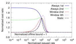
Figure 1. Cost ratios for an exponential inter-request time distribution and $W=T=R$.

Distributions with lower variability: Erlang results are obtained by using equations (18) and (19) to substitute for $E[a_{i}]$, $F(t)$ and the integral of $F(t)$ in equations (52), (7.2), (59), (67), and then simplifying. It is straightforward to show that, for any $k\geq 1$, the cost ratios for each of the policies in the limiting cases of $\lambda\rightarrow 0$ and $\lambda\rightarrow\infty$ are the same as for exponentially distributed inter-request times.

Results for deterministic inter-request times are obtained by using equations (21) and (22) to substitute into equations (52), (7.2), (59), (67), taking limits (when needed), and simplifying the expressions on a case-by-case basis. Again, the cost ratios for each of the policies in the limiting cases of $\lambda\rightarrow 0$ and $\lambda\rightarrow\infty$ are the same as for exponentially distributed inter-request times. Figure 2 shows the cost ratio results for Erlang and deterministic inter-request times. Note in particular how the peak cost ratio for single-window on $M^{th}$, with $M\geq 2$, reduces as $k$ increases and inter-request times become increasingly deterministic (far-right sub figure).

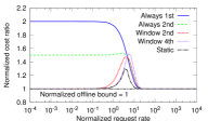
(a) Erlang, $k=2$

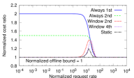
(b) Erlang, $k=4$

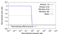
(c) Deterministic

Figure 2. Cost ratios for low variability inter-request time distributions and $W=T=R$.

Pareto: Results for Pareto inter-request time distributions are obtained using equations (24), (25) and (28) to substitute for $E[a_{i}]$, $F(t)$ and the integral of $F(t)$ in equations (52), (7.2), (59), and (67). Figure 3 shows cost ratio results for three different values of $\alpha$. We note that (as per Theorem 6.6), static baseline performs very poorly when $\alpha\rightarrow 1$ (and $t_{m}$ is small). This is illustrated by the large peak cost ratio in Figure 3(a), where $\alpha=1.1$. For larger $\alpha$ (e.g., $\alpha=2$ in Figure 3(c)), this peak reduces substantially. Otherwise, the results are similar as for the other inter-request distributions in that the maximum observed peaks are for always on $1^{st}$, and in that single-window on $2^{nd}$ has a tighter bound than single-window on $4^{th}$, suggesting that single-window on $2^{nd}$ with $T=R$ is a good choice.

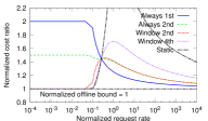
(a) $\alpha=1.1$

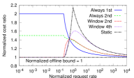
(b) $\alpha=1.25$

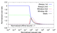
(c) $\alpha=2$

Figure 3. Cost ratios for Pareto inter-request time distributions and $W=T=R$.

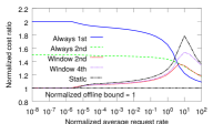
(a) Pareto $\alpha=1.25$

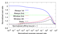
(b) Exponential

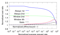
(c) Erlang $k=4$

Figure 4. Multi-file analysis for different inter-request time distributions; Zipf popularity distribution (frequency of requests to file $i$ proportional to $1/i^{\gamma}$, $\gamma=1$, and $1,000,000$ files).

9. Multi-file evaluation

Thus far we have focused primarily on deriving analytic expressions and insights based on the single file case. In this section, we complement this analysis with both analytic (Section 9.1) and trace-based (Section 9.2) evaluations for the multi-file case.

Throughout the section the different cache on $M^{th}$ request policies use the threshold values $W=T=R$. Being the optimal worst-case choices, they are natural choices for this context, since predicting individual object popularities is difficult and object popularities in practice typically change over time.

9.1. Heavy-tailed popularity analysis

File object popularities are typically highly skewed (Gill et al., 2007; Zink et al., 2009; Maggs and Sitaraman, 2015; Carlsson and Eager, 2017). For this analysis, we consider the delivery cost for a cache when the file object popularity is Zipf distributed with parameter $\gamma$ (i.e., the frequency of requests to the $i^{\textrm{th}}$ most popular file object is proportional to $\frac{1}{i^{\gamma}}$) and all file objects have the same size. Since both storage and bandwidth cost in our model scale proportional to the file size, results for variable-sized files could be easily obtained simply by weighting the costs for each file according to the file size.

Figure 4 shows the cost ratio for the different policies as a function of the normalized average request rate, when $\gamma$=$1$ and there are $1,000,000$ files. To allow comparisons with the single-file case, we include results for three forms for the inter-request time distribution of each file: Pareto with $\alpha$=$1.25$ (Figure 4(a)), exponential (Figure 4(b)), and Erlang with $k$=$4$ (Figure 4(c)). Different files have different distribution parameter values (value of $t_{m}$ for Pareto, $\lambda$ for exponential and Erlang) so as to achieve the desired Zipf request frequency distribution. Results for Zipf popularity distributions with $\gamma$=$0.75$ and $\gamma$=$1.25$ are very similar.

We note that window on $M^{th}$ with $M=2$ has a peak cost-ratio compared to the offline optimal of 1.4, and significantly outperforms the always on $M^{th}$ policies. These results again clearly highlight the value of a more selective insertion policy.

Also important to note is the small gap between the static baseline policy and the window-based policies for exponential (Figure 4(b)) and Erlang (Figure 4(c)) distributed inter-request times, and that the window-based policies outperform the static baseline policy when inter-request times are Pareto distributed (Figure 4(a)). The static baseline policy optimizes its selection between always caching, and never caching, each file according to that file’s inter-request time distribution. This yields minimum cost among all online policies for the distributions considered in Figures 4(b) and 4(c). Yet, window on $2^{nd}$ and window on $4^{th}$ achieve close to this online bound, while treating all files the same. These results are highly encouraging and show that the same policy can be used for all files, regardless of popularity and the form of the inter-request time distribution.

While the cost gap generally is small, we note that the region over which the window-based policies (and other online policies) leave a significant gap compared to the offline optimal is substantially wider for the multi-file case than for the single file case. For example, for exponential inter-request times, there is a significant gap in the multi-file case (Figure 4(b)) for normalized average request rate values from about $10^{-5}$ to $10^{2}$, while a significant gap in the single file case (Figure 1) appears only for request rate values from about $10^{-2}$ to $10$. This is explained by the fact that in the multi-file case, files have widely-varying request rates, and over a wide range of average request rates there are files whose individual request rate falls in the region in which, in the single file case, there is a substantial gap compared to the offline optimal. Interestingly, the size of the set of files contributing to this gap will differ for different average request rates. For example, at low average request rates, there will be a small set of relatively popular files contributing to the gap. However, due to the skew in popularity, this set will account for a disproportionate share of the total request volume. The small step around $10^{-6}$ to $10^{-5}$ is due to the most popular files entering this region. At high average request rates, the number of files whose individual request rate falls in the region with a substantial gap increases, but these files now account for a disproportionately smaller share of the total request rate, an effect that reduces the size of the peak gap for the cache on $M^{th}$ request policies. Note that for the always on $M^{th}$ policies, the worst-case gap (at low request rates) is the same as for the single file case. However, the worst-case asymptotes are not approached until the request rates for all files are low (which happens when the average request rate falls somewhere between $10^{-4}$ and $10^{-6}$, depending on the distribution skew).

9.2. Trace-based evaluation

For our trace-based analysis, we use a 20 month long trace capturing all YouTube video requests from a campus network with 35,000 faculty, staff, and students. The trace spans between July 1, 2008, and February 28, 2010, and contains roughly 5.5 million requests to 2.4 million unique YouTube videos (Carlsson and Eager, 2017). This type of traffic is particularly interesting since file popularities are ephemeral and there typically is a long tail of less popular files that individually are viewed very few times, but that as an aggregate contribute to a significant part of the total views. For example, in the university dataset, 90% of the videos are requested three or fewer times, and yet these videos make up half of the views observed on campus.

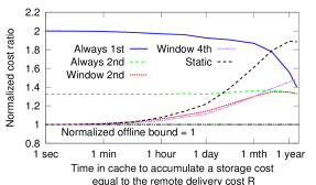
Figure 5. Trace-based simulation results with $W=T=R$.

Figure 5 shows summary results for our trace-based simulations. Here, for each policy we plot the ratio of the total aggregate delivery cost across all videos divided by the corresponding delivery cost using the offline optimal policy, as a function of the time that a file would need to be stored in cache to accumulate remote delivery cost $R$. With the unit normalization described in Section 2, $W=T=R$ implies that storing a file in cache for $W=T$ time units would incur a cost equal to $R$, and so the x-axis values also correspond to the window sizes $W$ and $T$. For the static baseline policy, we make the optimistic assumptions that (i) an oracle can be used to determine which of always local and always remote will perform best for each individual video, and (ii) in the case of always local the file object is not retrieved until the time of the first request (at a cost $R$). In practice, such knowledge would not be available to any online policy. Yet, the window on $M^{th}$ policies significantly outperform the static baseline policy. This shows the importance of being selective in what is added to the cache.

Due to the dominance of videos that see few requests, the results resemble the multi-file analytic results for lower average request rates, with the window-based cache on $M^{th}$ request policies performing the best. For example, with 5.5 million requests to 2.4 million videos over a 20 month period, a window size $W=T$ of 20 months would imply a normalized average request rate, as used on the x-axes in Figures 1-4, of 2.3. Furthermore, window on $M^{th}$ with $M=4$ is a slightly better choice than $M=2$ for shorter than month-long caching thresholds $W=T=R$, whereas for longer thresholds, $M=2$ is the better policy.

Much of the improvements over the always on 1^st policy, come from the window on $M^{th}$ policies, with intermediate $M$, requiring smaller storage. For example, with a one-week threshold the average cache size at object evictions (across all object evictions) reduces from 153,729 objects (with always on 1^st) to 57,652 ($M=2$) and 29,034 ($M=4$). The corresponding values for a 30-day (“one month” in Figure 5) threshold are: 343,139, 150,364 and 58,170. Here, we also note that the variance in cache size needed over these time scales is relatively small, despite significant seasonal request volume variations in the trace (e.g., comparing summer breaks vs. regular term (Carlsson and Eager, 2017)). For example, in the case of the one-month threshold, the ratios of the maximum observed cache size to the minimum observed cache size at any two cache evictions instances (across the full 20-month trace) for these three policies are: 2.67, 2.21, and 2.02, respectively.

To better understand (i) which files contribute most of the absolute cost and (ii) which files contribute most of the cost inflation (as seen in Figure 5) compared to the offline optimal bound, Figure 6 breaks down the cost due to videos of different popularities. Figure 6(a) shows the costs of the different policies associated with the videos with more than 20 views, expressed relative to the total offline optimal bound cost. This set contains 0.95% of the unique videos and is responsible for 22.8% of the views. Figures 6(b) and 6(c) show the corresponding results for the videos that have 4-20 views and 1-3 views over the duration of the 20-month long trace, respectively. These two sets contain 9.0% and 90% of the unique videos, and are responsible for 27.6% and 49.6% of the views, respectively.

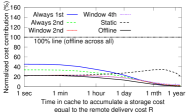
(a) Top (more than 20 views)

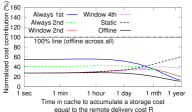
(b) Middle (4-20 views)

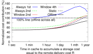
(c) Tail (1-3 views)

Figure 6. Breakdown of cost contributions of the videos belonging to three different popularity categories. (University dataset.)

These figures also show that the advantage of using window-based, rather than purely counter-based, cache on $M^{th}$ request policies is consistent across the three popularity classes, and that the fraction of the offline optimal caching cost that the long-tail of less popular videos contributes increases as the thresholds increase (and more videos are cached). Much of the penalty of the static baseline policy is associated with the more popular videos (comparing Figures 6(a) and (b) to Figure 6(c)), and longer thresholds, likely due to this policy not capturing the ephemeral popularity of these videos.

Interestingly, even when the time in cache to accumulate a storage cost equal to the remote delivery cost $R$ is very small, the few timers (with 1-3 views) still contribute approximately 50% of the total cost for all policies, except for always on $1^{st}$ and always on $2^{nd}$, for which the contribution is even higher. Overall, these results show the importance of selective caching policies such as the window-based cache on $M^{th}$ request policies analyzed in this paper.

10. Related work

Most existing caching works focus on replacement policies (Podlipnig and Böszörmenyi, 2003; Barish and Obraczke, 2000). However, recently it has been shown that the cache insertion policies play a very important factor in reducing the total delivery costs (Maggs and Sitaraman, 2015; Carlsson and Eager, 2017). Motivated by these works, this paper focuses on the delivery cost differences between different selective cache insertion policies.

Few papers (regardless of replacement policy) have modeled selective cache insertion policies such as cache on $M^{th}$ request. This class of policies is motivated by the risk of cache pollution due to ephemeral content popularity and the long tail of one-timers (one-hit wonders) observed in edge networks (Gill et al., 2007; Zink et al., 2009; Maggs and Sitaraman, 2015; Carlsson and Eager, 2017). Recent works including trace-based evaluations of cache on $M^{th}$ request policies (Maggs and Sitaraman, 2015; Carlsson and Eager, 2017). Carlsson and Eager (Carlsson and Eager, 2017) also present simple analytic models for hit and insertion probabilities. However, in contrast to the analysis presented here, they assume that content is not evicted until interest in the content has expired. Garetto et al. (Garetto et al., 2016; Martina et al., 2014) and Gast and Van Houdt (Gast and Van Houdt, 2015; Gast and Houdt, 2016) present TTL-based recurrence expressions and approximations for two variations of cache on $M^{th}$ request, referred to as k-LRU and LRU(m) in their works. However, none of these works present performance bounds or consider the total delivery cost. In contrast, we derive both worst-case bounds and average-case analysis under a cost model that captures both bandwidth and storage costs.

Finally, it is important to note that TTL-based eviction policies (Jung et al., 2003; Bahat and Makowski, 2005) (and variations thereof (Carlsson and Eager, 2018)) have been found useful for approximating the performance of capacity-driven replacement policies such as LRU (Che et al., 2002; Fricker et al., 2012; Bianchi et al., 2013; Berger et al., 2014; Garetto et al., 2016). Our results may therefore also provide insight for the case in which a content provider uses a fixed-sized cache. Generalizations of the TTL-based Che-approximation (Che et al., 2002) and TTL-based caches in general have proven useful to analyze individual caches (Che et al., 2002; Fricker et al., 2012; Bianchi et al., 2013; Berger et al., 2014; Garetto et al., 2016), networks of caches (Fofack et al., 2012; Fofack et al., 2014; Fofack et al., 2014; Berger et al., 2014; Garetto et al., 2016), and to optimize different system designs (Carlsson et al., 2014; Dehghan et al., 2016; Ferragut et al., 2016; Ma and Towsley, 2015).

As we show here, elasticity assumptions can also be a powerful toolbox for deriving tight worst-case bounds and exact average-case cost ratios of different policies. Furthermore, as discussed in Section 9.1, since both storage costs and bandwidth costs are proportional to the file sizes, the results can also easily be extended to scenarios with variable sized objects, at no additional computational cost. In contrast, just finding lower and upper bounds for the cache miss rate of the optimal offline policy is computationally expensive when caches are non-elastic (Berger et al., 2018) and even simple LRU is hard to analyze under non-elastic constraints (King III, 1971; Dan and Towsley, 1990).

11. Conclusions

In this paper, we consider the delivery costs of a content provider that wants to minimize its delivery costs under the assumptions that the resources it requires are elastic, the content provider only pays for the resources that it consumes, and costs are proportional to the resource usage. Under these assumptions, we first derived worst-case bounds for the optimal cost and competitive cost-ratios of different classes of cache on $M^{th}$ request cache insertion policies. Second, we derived explicit average cost expressions and bounds under arbitrary inter-request time distributions, as well as for short-tailed inter-request time distributions (deterministic, Erlang, and exponential) and heavy-tailed inter-request distributions (Pareto). Finally, using these analytic results, we have presented numerical evaluations and cost comparisons that reveal insights into the relative cost performance of the policies. Interestingly, we have found that single-window on $M^{th}$ with an intermediate $M$ (e.g., 2-4) and $T=R$ achieves most of the benefits of this class of policies. Choosing $T=R$ guarantees a worst-case competitive ratio of $M+1$ (compared to the optimal offline policy), but typically performs much better. For example, we have found that this policy with $M=2$ closely tracks the online optimal policy for the short-tailed inter-request time distributions, and significantly outperforms the standard non-selective policy always on $1^{st}$ across all inter-request distributions considered here. Using $M=4$ can result in further improvements for lower request rates (e.g., as associated with a long tail of less popular file objects), but performs somewhat worse when request rates are intermediate (where the gap between the online and offline policies is the greatest). These results suggest that cache on $2^{nd}$ optimized to minimize worst-case costs provides good average performance, making it an attractive choice for a wide range of practical conditions where request rates of individual objects typically are not known and can quickly change.

Appendix A Additional worst-case proofs

A.1. Proof Theorem 4.3: Always on $M^{th}$

We next prove Theorem 4.3, which specifies the worst-case properties of always on $M^{th}$.

Proof.

Case $T\leq R$: For $2\leq i\leq N$, let us define the following sets based on the operation of the always on $M^{th}$ policy: $S^{A}_{m}=\{i|a_{i}\leq R\land i$ is the $m^{th}$request$\}$, $S^{C}_{m}=\{i|R<a_{i}\land i$ is the $m^{th}$request$\}$, where we label request $i$ as the $m^{th}$ request when it is the $m^{th}$ request to the object since the object was removed from the cache most recently or the request sequence started. For the case that the previous request put the object into the cache or the object remained in the cache, we define the following sets: $S^{A}_{+}=\{i|a_{i}\leq T\land i\notin\cup_{m=2}^{M}S^{A}_{m}\}$, $S^{B}_{+}=\{i|T<a_{i}\leq R\land i\notin\cup_{m=2}^{M}S^{A}_{m}\}$, and $S^{C}_{+}=\{i|R<a_{i}\land i\notin\cup_{m=2}^{M}S^{C}_{m}\}$. Note that the set $S^{A}_{+}$ corresponds to cache hits using the always on $M^{th}$ policy, and that sets $S^{B}_{+}$ and $S^{C}_{+}$ corresponds to cases where the counter is reset after the object has been removed from the cache (and the cache incurred an extra storage cost $T$ after most recent prior request).

Now, for an arbitrary request sequence $\mathcal{A}$, we can bound the cost of the always on $M^{th}$ policy as follows: $C^{always}_{M,T}\leq R+\sum_{m=2}^{M}|S^{A}_{m}|R+\sum_{m=2}^{M}|S^{C}_{m}|R+\sum_{i\in S^{A}_{+}}a_{i}+(|S^{B}_{+}|+|S^{C}_{+}|)(R+T)+T$, where the final $T$ only is needed if the last request in the sequence is from set $S^{A}_{+}$. (In all other cases the bound becomes loose.) Now, noting that (i) $|S^{A}_{M}|+|S^{C}_{M}|\leq|S^{A}_{M-1}|+|S^{C}_{M-1}|\leq...\leq|S^{A}_{2}|+|S^{C}_{2}|$, (ii) $\sum_{m=2}^{M}(|S^{A}_{m}|+S^{C}_{m}|)\leq(M_{1})(|S^{A}_{2}|+|S^{C}_{2}|)$, and (iii) $|S^{B}_{+}|+|S^{C}_{+}|\leq|S^{A}_{2}|+|S^{C}_{2}|$, we can write $C^{always}_{M,T}\leq R+M(|S^{A}_{2}|+|S^{C}_{2}|)R+(|S^{A}_{2}|+|S^{C}_{2}|)T+\sum_{i\in S^{A}_{+}}a_{i}+T$.

For the optimal offline policy, we note that all requests in the sets $S^{A}_{m}$, $S^{A}_{+}$, $S^{B}_{+}$ correspond to cache hits (associated with an extra storage cost $a_{i}$), whereas the remaining requests are cache misses (associated with a remote access cost $R$). Therefore, for the same request sequence $\mathcal{A}$, the cost of the optimal (offline) policy can be bounded as follows: $C_{opt}^{offline}=R+\sum_{i\in{\cup_{m=2}^{M}S^{A}_{m}}}a_{i}+\sum_{m=2}^{M}|S^{C}_{m}|R+\sum_{i\in S^{A}_{+}}a_{i}+\sum_{i\in S^{B}_{+}}a_{i}+|S^{C}_{+}|R$ $\geq R+\sum_{m=2}^{M}R|S^{C}_{m}|+T|S^{B}_{+}|+|S^{C}_{+}|R+\sum_{i\in S^{A}_{+}}a_{i}$ $\geq R+T(|S^{A}_{2}|+|S^{C}_{2}|)+\sum_{i\in S^{A}_{+}}a_{i}$. Here, we have used that (i) $\sum_{i\in{\cup_{m=2}^{M}S^{A}_{m}}}a_{i}\geq 0$, (ii) $\sum_{i\in S^{B}_{+}}a_{i}\geq T|S^{B}_{+}|$, (iii) $\sum_{i\in S^{C}_{+}}a_{i}\geq R|S^{C}_{+}|$, and (vi) $T|S^{B}_{+}|+|S^{C}_{+}|R\geq T(|S^{B}_{+}|+|S^{C}_{+}|)=T(|S^{A}_{2}|+|S^{A}_{2}|$). Taking the ratio

$$\frac{C^{always}_{M,T}}{C_{opt}^{offline}} \leq\frac{R+M(|S^{A}_{2}|+|S^{C}_{2}|)R+(|S^{A}_{2}|+|S^{C}_{2}|)T+\sum_{i\in S^{A}_{+}}a_{i}+T}{R+T(|S^{A}_{2}|+|S^{C}_{2}|)+\sum_{i\in S^{A}_{+}}a_{i}}$$

(72) $$\leq\frac{R+M(|S^{A}_{2}|+|S^{C}_{2}|)R+(|S^{A}_{2}|+|S^{C}_{2}|)T+T}{R+T(|S^{A}_{2}|+|S^{C}_{2}|)},$$

it is easy to show that the worst case scenario happens with $|S^{A}_{2}|+|S^{C}_{2}|\rightarrow\infty$ and that the worst-case bound is minimized by setting $T=R$. (To see this, note that $\frac{d}{dx}(\frac{R+MRx+Tx+T}{R+Tx})=\frac{MR^{2}-T^{2}}{(R+Tx)^{2}}\geq 0$.) In this case the worst-case ratio reduces to $(M+1)$.

Finally, we show that this ratio is achievable by a request pattern in which requests occurs in batches of $M$ requests, with consecutive batches spaced by more than $R$ time units. In this case, we have $a_{i}=0$ for all $i\in S^{A}_{m}$, $|S^{A}_{+}|=|S^{B}_{+}|=|S^{C}_{+}|=|S^{B}_{m}|=0$ for all $m$, and $|S^{A}_{m}|=|S^{C}_{+}|$ for all $m$. In each batch cycle, the always on $M^{th}$ policy downloads the object $M$ times from the server and keeps it in the cache for $R$ time units (at a total cost of $(M+1)R$ per batch). In contrast, the optimal offline policy downloads a single copy (at cost $R$), serves all $M$ requests using this copy, and then instantaneously deletes the copy (to avoid storage costs).

Case $R\leq T$: Let us define the following sets for $2\leq i\leq N$: $G^{A}_{m}=\{i|a_{i}\leq R\land i$ is the $m^{th}$request$\}$, $G^{C}_{m}=\{i|R<a_{i}\land i$ is the $m^{th}$request$\}$, where $2\leq m\leq M$, and $G^{A}_{+}=\{i|a_{i}\leq R\land i\notin\cup_{m=2}^{M}G^{A}_{m}\}$, $G^{B}_{+}=\{i|R<a_{i}\leq T\land i\notin\cup_{m=2}^{M}G^{C}_{m}\}$, and $G^{C}_{+}=\{i|T<a_{i}\land i\notin\cup_{m=2}^{M}G^{C}_{m}\}$. With these sets, only the requests in sets $G^{A}_{+}$ and $G^{B}_{+}$ correspond to cache hits (with associated cost $a_{i}$) with the always on $M^{th}$ policy. Furthermore, with this policy, the requests in set $G^{C}_{+}$ corresponds to cases where the counter is reset after the object has been removed from the cache. These cache misses are therefore associated with an extra storage cost $T$ (corresponding to the time the object was in the cache without being requested again after the most recent earlier request). Now, for an arbitrary request sequence $\mathcal{A}$, we can bound the cost of this policy as follows: $C^{always}_{M,T}\leq R+\sum_{m=2}^{M}|G^{A}_{m}|R+\sum_{m=2}^{M}|G^{C}_{m}|R+\sum_{i\in G^{A}_{+}}a_{i}+\sum_{i\in G^{B}_{+}}a_{i}+|G^{C}_{+}|(R+T)+T$. Now, noting that (i) $\sum_{m=2}^{M}(|G^{A}_{m}|+|G^{C}_{m}|)\leq(M-1)(|G^{A}_{2}|+|G^{C}_{2}|)$, (ii) $|G^{C}_{+}|=|G^{A}_{2}|+|G^{C}_{2}|$, (iii) $\sum_{i\in G^{B}_{+}}a_{i}\leq|G^{B}_{+}|T$, we can write $C^{always}_{M,T}\leq R+M|G^{C}_{+}|R+(|G^{C}_{+}|)T+|G^{B}_{+}|T+\sum_{i\in G^{A}_{+}}a_{i}+T$. Similarly, for the same request sequence $\mathcal{A}$, the cost of the optimal offline policy can be bounded as follows: $C_{opt}^{offline}=R+\sum_{m=2}^{M}\sum_{i\in G^{A}_{m}}a_{i}+\sum_{m=2}^{M}|G^{C}_{m}|R+\sum_{i\in G^{A}_{+}}a_{i}+|G^{B}_{+}|R+|G^{C}_{+}|R$ $\geq R+|G^{B}_{+}|R+|G^{C}_{+}|R+\sum_{i\in G^{A}_{+}}a_{i}$, where we have used that (i) $\sum_{i\in G^{A}_{m}}a_{i}\geq 0$, and (ii) $|G^{C}_{m}|\geq 0$. Taking the ratio

$$\frac{C^{always}_{M,T}}{C_{opt}^{offline}} \leq\frac{R+M|G^{C}_{+}|R+|G^{C}_{+}|T+|G^{B}_{+}|T+\sum_{i\in G^{A}_{+}}a_{i}+T}{R+|G^{B}_{+}|R+|G^{C}_{+}|R+\sum_{i\in G^{A}_{+}}a_{i}}$$

(73) $$\leq\frac{R+M|G^{C}_{+}|R+|G^{C}_{+}|T+|G^{B}_{+}|T+T}{R+|G^{B}_{+}|R+|G^{C}_{+}|R}$$

it can be seen that, as earlier, this ratio is minimized when $T=R$, for which it is bounded by $(M+1)$ when $|G^{B}_{+}|=0$ and $(|G^{C}_{+}|)\rightarrow\infty$. (To see this, note that $\frac{d}{dx}(\frac{R+MRx+Tx+BT+T}{R+BR+Rx})=\frac{BM+M-1}{(B+x+1)^{2}}\geq 0$.) It is trivial to see that the same request pattern (but with batches separated by more than $T$ rather than $R$) results in the worst case being achieved. This shows that the bound is tight. ∎

A.2. Proof Theorem 4.4: Single-window on $M^{th}$

We next prove Theorem 4.4, which specifies the worst-case properties of single-window on $M^{th}$.

Proof.

Case $T\leq R$: For $2\leq i\leq N$, let us define the following sets based on the operation of the single-window on $M^{th}$ policy: $S^{A}_{m}=\{i|a_{i}\leq T\land i$ is an $m^{th}$ candidate$\}$, $S^{B}_{m}=\{i|T<a_{i}\leq R\land i$ is an $m^{th}$ candidate$\}$, and $S^{C}_{m}=\{i|R<a_{i}\land i$ is an $m^{th}$ candidate$\}$, where we say that a request is an $m^{th}$ candidate whenever the previous request in the request sequence to the object set the counter to $(m-1)$. Note that the first overall request and the first request after the object has been removed from the cache always sets the counter to one (and the next request to the object hence becomes a $2^{nd}$ candidate). For the case that the previous request put the object into the cache or the object remained in the cache, we define the following sets: $S^{A}_{+}=\{i|a_{i}\leq T\land i\notin\cup_{m=2}^{M}S^{A}_{m}\}$, $S^{B}_{+}=\{i|T<a_{i}\leq R\land i\notin\cup_{m=2}^{M}S^{B}_{m}\}$, and $S^{C}_{+}=\{i|R<a_{i}\land i\notin\cup_{m=2}^{M}S^{C}_{m}\}$. Note that the requests in the set $S^{A}_{+}$ corresponds to cache hits using the single-window on $M^{th}$ policy, and that sets $S^{B}_{+}$ and $S^{C}_{+}$ correspond to cases where the counter is reset after the object has been removed from the cache (and the cache incurred an extra storage cost $T$ after the most recent prior request).

Now, for an arbitrary request sequence $\mathcal{A}$, we can bound cost of the single-window on $M^{th}$ policy as follows: $C^{window}_{M,T}\leq R+\sum_{m=2}^{M}|S^{A}_{m}|R+\sum_{m=2}^{M}|S^{B}_{m}|R+\sum_{m=2}^{M}|S^{C}_{m}|R+\sum_{i\in S^{A}_{+}}a_{i}+(|S^{B}_{+}|+|S^{C}_{+}|)(R+T)+T$, where the final $T$ only is needed if the last request in the sequence is from set $S^{A}_{+}$. (In all other cases the bound becomes loose.) Now, noting that (i) $|S^{A}_{M}|\leq|S^{A}_{M-1}|\leq...\leq|S^{A}_{2}|$, (ii) $\sum_{m=2}^{M}|S^{A}_{m}|\leq(M_{1})|S^{A}_{2}|$, (iii) $\sum_{m=2}|S^{B}_{m}|+\sum_{m=2}|S^{C}_{m}|+|S^{B}_{+}|+|S^{C}_{+}|\leq|S^{A}_{2}|$, and (iv) $|S^{B}_{+}|+|S^{C}_{+}|\leq|S^{A}_{2}|$, we can write $C^{window}_{M,T}\leq R+M|S^{A}_{2}|R+|S^{A}_{2}|T+\sum_{i\in S^{A}_{+}}a_{i}+T$.

For the optimal offline policy, we note that all requests in the sets $S^{A}_{m}$, $S^{B}_{m}$, $S^{A}_{+}$, $S^{B}_{+}$ correspond to cache hits (associated with an extra storage cost $a_{i}$), whereas the remaining requests are cache misses (associated with a remote access cost $R$). Therefore, for the same request sequence $\mathcal{A}$, the cost of the optimal (offline) policy can be bounded as follows: $C_{opt}^{offline}=R+\sum_{i\in{\cup_{m=2}^{M}S^{A}_{m}}}a_{i}+\sum_{i\in{\cup_{m=2}^{M}S^{B}_{m}}}a_{i}+\sum_{m=2}^{M}|S^{C}_{m}|R+\sum_{i\in S^{A}_{+}}a_{i}+\sum_{i\in S^{B}_{+}}+|S^{C}_{+}|R\geq R+T(\sum_{m=2}^{M}|S^{B}_{m}|+|S^{B}_{+}|)+R(\sum_{m=2}^{M}|S^{C}_{m}|+|S^{C}_{+}|)+\sum_{i\in S^{A}_{+}}a_{i}\geq R+|S^{A}_{2}|T+\sum_{i\in S^{A}_{+}}a_{i}$. Here, we have used that (i) $\sum_{i\in{\cup_{m=2}^{M}S^{A}_{m}}}a_{i}\geq 0$, (ii) $\sum_{i\in S^{B}_{m}}a_{i}\geq T|S^{B}_{m}|$, (iii) $\sum_{i\in S^{C}_{m}}a_{i}\geq T|S^{C}_{m}|$, (iv) $\sum_{i\in S^{B}_{+}}a_{i}\geq T|S^{B}_{+}|$, (v) $\sum_{i\in S^{C}_{+}}a_{i}\geq T|S^{C}_{+}|$, (vi) $T\sum_{m=2}^{M}|S^{B}_{m}|+R\sum_{m=2}^{M}|S^{C}_{m}|+T|S^{B}_{+}|+R|S^{C}_{+}|\geq T(\sum_{m=2}^{M}|S^{B}_{m}|+\sum_{m=2}^{M}|S^{C}_{m}|+|S^{B}_{+}|+|S^{C}_{+}|)=T|S^{A}_{2}|$. Taking the ratio

$$\frac{C^{window}_{M,T}}{C_{opt}^{offline}} \leq\frac{R+M|S^{A}_{2}|R+|S^{A}_{2}|T+\sum_{i\in S^{A}_{+}}a_{i}+T}{R+T|S^{A}_{2}|+\sum_{i\in S^{A}_{+}}a_{i}}$$

(74) $$\leq\frac{R+M|S^{A}_{2}|R+|S^{A}_{2}|T+T}{R+T|S^{A}_{2}|}$$

it is easy to show that the worst case scenario happens with $|S^{A}_{2}|\rightarrow\infty$ and that the worst-case bound is minimized by setting $T=R$. In this case the worst-case ratio reduces to $(M+1)$.

Finally, we show that this ratio is achievable by a request pattern in which requests occurs in batches of $M$ requests, with consecutive batches spaced by more than $R$ time units. In this case, we have $a_{i}=0$ for all $i\in S^{A}_{m}$, $|S^{A}_{+}|=|S^{B}_{+}|=|S^{C}_{+}|=|S^{B}_{m}|=0$ for all $m$, and $|S^{A}_{m}|=|S^{C}_{+}|$ for all $m$. In each batch cycle, the single-window on $M^{th}$ policy downloads the object $M$ times from the server and keeps it in the cache for $R$ time units (at a total cost of $(M+1)R$ per batch). In contrast, the optimal offline policy downloads a single copy (at cost $R$), serves all $M$ requests using this copy, and then instantaneously deletes the copy (to avoid storage costs).

Case $R\leq T$: Let us define the following sets for $2\leq i\leq N$: $G^{A}_{m}=\{i|a_{i}\leq R\land i$ is an $m^{th}$ candidate$\}$, $G^{B}_{m}=\{i|R<a_{i}\leq T\land i$ is an $m^{th}$ candidate$\}$, $G^{C}_{m}=\{i|T<a_{i}\land i$ is an $m^{th}$ candidate$\}$, where $2\leq m\leq M$, and $G^{A}_{+}=\{i|a_{i}\leq R\land i\notin\cup_{m=2}^{M}G^{A}_{m}\}$, $G^{B}_{+}=\{i|R<a_{i}\leq T\land i\notin\cup_{m=2}^{M}G^{B}_{m}\}$, and $G^{C}_{+}=\{i|T<a_{i}\land i\notin\cup_{m=2}^{M}G^{C}_{m}\}$. With these sets, only the requests in the sets $G^{A}_{+}$ and $G^{B}_{+}$ correspond to cache hits (with associated cost $a_{i}$) with the single-window on $M^{th}$ policy. Furthermore, with this policy, the requests in set $G^{C}_{+}$ correspond to cases where the counter is reset after the object has been removed from the cache. These cache misses are therefore associated with an extra storage cost $T$ (corresponding to the time the object was in the cache without being requested again after the most recent earlier request). Now, for an arbitrary request sequence $\mathcal{A}$, we can bound the cost of this policy as follows: $C^{window}_{M,T}\leq R+\sum_{m=2}^{M}|G^{A}_{m}|R+\sum_{m=2}^{M}|G^{B}_{m}|R+\sum_{m=2}^{M}|G^{C}_{m}|R+\sum_{i\in G^{A}_{+}}a_{i}+\sum_{i\in G^{B}_{+}}a_{i}+|G^{C}_{+}|(R+T)+T$. Now, noting that (i) $\sum_{m=2}^{M}(|G^{A}_{m}|+|G^{B}_{m}|)\leq(M_{1})(|G^{A}_{2}|+|G^{B}_{2}|)$, (ii) $\sum_{m=2}^{M}|G^{C}_{m}|+|G^{C}_{+}|=|G^{A}_{2}|+|G^{B}_{2}|$, (iii) $|G^{C}_{+}|=|G^{A}_{2}|+|G^{B}_{2}|-\sum_{m=2}^{M}|G^{C}_{m}|\leq|G^{A}_{2}|+|G^{B}_{2}|$, and (iv) $\sum_{i\in G^{B}_{+}}a_{i}\leq|G^{B}_{+}|T$, we can write $C^{window}_{M,T}\leq R+M(|G^{A}_{2}|+|G^{B}_{2}|)R+(|G^{A}_{2}|+|G^{B}_{2}|)T+|G^{B}_{+}|T+\sum_{i\in S^{A}_{+}}a_{i}+T$. Similarly, for the same request pattern $\mathcal{A}$, the cost of the optimal offline policy can be bounded as follows: $C_{opt}^{offline}=R+\sum_{m=2}^{M}\sum_{i\in G^{A}_{m}}a_{i}+\sum_{m=2}^{M}|G^{B}_{m}|R+\sum_{m=2}^{M}|G^{C}_{m}|R+\sum_{i\in G^{A}_{+}}a_{i}+|G^{B}_{+}|R+|G^{C}_{+}|R\leq R+(|G^{A}_{2}|+|G^{B}_{2}|)R+|G^{B}_{+}|T+\sum_{i\in S^{A}_{+}}a_{i}$, where we have used that (i) $\sum_{i\in G^{A}_{m}}a_{i}\geq 0$, (ii) $|G^{B}_{m}|\leq 0$, and (iii) $\sum_{m=2}^{M}|G^{C}_{m}|+|G^{C}_{+}|=|G^{A}_{2}|+|G^{B}_{2}|$. Taking the ratio

$$\frac{C^{window}_{M,T}}{C_{opt}^{offline}} \leq{\textstyle{\frac{R+M(|G^{A}_{2}|+|G^{B}_{2}|)R+(|G^{A}_{2}|+|G^{B}_{2}|)T+|G^{B}_{+}|T+\sum_{i\in S^{A}_{+}}a_{i}+T}{R+(|G^{A}_{2}|+|G^{B}_{2}|)R+|G^{B}_{+}|T+\sum_{i\in S^{A}_{+}}a_{i}}}}$$

(75) $$\leq\frac{R+M(|G^{A}_{2}|+|G^{B}_{2}|)R+(|G^{A}_{2}|+|G^{B}_{2}|)T+|G^{B}_{+}|T+T}{R+(|G^{A}_{2}|+|G^{B}_{2}|)R+|G^{B}_{+}|T}.$$

it is easy to show that, as earlier, this ratio is minimized when $T=R$, for which it is bounded by $(M+1)$ when $|G^{B}_{+}|=0$ and $(|G^{A}_{2}|+|G^{B}_{2}|)\rightarrow\infty$. It is trivial to see that the same request pattern (but with batches separated by more than $T$ rather than $R$) results in the worst case being achieved. This shows that the bound is tight.

∎

A.3. Proof Theorem 4.5: Dual-window on $2^{nd}$

We next prove Theorem 4.5, which specifies the worst-case properties of dual-window on $2^{nd}$.

Proof.

Case $W\leq T\leq R$: Let us define the following sets for $2\leq i\leq N$: $S^{A}_{2}=\{i|a_{i}<W\land i~{}\textrm{is~{}a~{}2}^{nd}~{}\textrm{candidate}\}$, $S^{B}_{2}=\{i|W\leq a_{i}<T\land i~{}\textrm{is~{}a~{}2}^{nd}~{}\textrm{candidate}\}$, $S^{C}_{2}=\{i|T\leq a_{i}<R\land i~{}\textrm{is~{}a~{}2}^{nd}~{}\textrm{candidate}\}$, $S^{D}_{2}=\{i|R\leq a_{i}\land i~{}\textrm{is~{}a~{}2}^{nd}~{}\textrm{candidate}\}$, $S^{A}_{+}=\{i|a_{i}<W\land i\notin S^{A}_{2}\}$, $B^{B}_{+}=\{i|W\leq a_{i}<T\land i\notin S^{B}_{2}\}$, $S^{C}_{+}=\{i|T\leq a_{i}<R\land i\notin S^{C}_{2}\}$, and $S^{D}_{+}=\{i|R\leq a_{i}\land i\notin S^{D}_{2}\}$. We can now write $C^{M=2}_{W,T}=R+(|S^{A}_{2}|+|S^{B}_{2}|+|S^{C}_{2}|+|S^{D}_{2}|)R+\sum_{i\in S^{A}_{+}}a_{i}+\sum_{i\in S^{B}_{+}}a_{i}+(|S^{C}_{+}|+|S^{D}_{+}|)(R+T)$, and $C_{opt}=R+\sum_{i\in S^{A}_{2}}a_{i}+\sum_{i\in S^{B}_{2}}a_{i}+\sum_{i\in S^{C}_{2}}a_{i}+|S^{D}_{2}|R+\sum_{i\in S^{A}_{+}}a_{i}+\sum_{i\in S^{B}_{+}}a_{i}+\sum_{i\in S^{C}_{+}}a_{i}+|S^{D}_{+}|R$. Now, noting that $|S^{C}_{+}|+|S^{D}_{+}|=|S^{A}_{2}|$, and making similar simplifications as in prior proofs, it is easy to show that:

(76) $$\frac{C^{window}_{M=2,W,T}}{C_{opt}^{offline}}\leq\frac{R+2|S^{A}_{2}|R+|S^{A}_{2}|T+|S^{B}_{2}|R+|S^{C}_{2}|R}{R+|S^{A}_{2}|T+|S^{B}_{2}|W+|S^{C}_{2}|T}.$$

This expression is minimized when $W\rightarrow T$ and $T\rightarrow R$. With these choices, the worst-case bound of 3 is achieved when $|S^{B}_{2}|=|S^{C}_{2}|=0$ and $|S^{A}_{2}|\rightarrow\infty$ (and the same worst-case request sequence as used for the single parameter version).

Case $W\leq R\leq T$: Let us define the following sets for $2\leq i\leq N$: $H^{A}_{2}=\{i|a_{i}<W\land i~{}\textrm{is~{}a~{}2}^{nd}~{}\textrm{candidate}\}$, $H^{B}_{2}=\{i|W\leq a_{i}<R\land i~{}\textrm{is~{}a~{}2}^{nd}~{}\textrm{candidate}\}$, $H^{C}_{2}=\{i|R\leq a_{i}<T\land i~{}\textrm{is~{}a~{}2}^{nd}~{}\textrm{candidate}\}$, $H^{D}_{2}=\{i|T\leq a_{i}\land i~{}\textrm{is~{}a~{}2}^{nd}~{}\textrm{candidate}\}$, $H^{A}_{+}=\{i|a_{i}<W\land i\notin H^{A}_{2}\}$, $H^{B}_{+}=\{i|W\leq a_{i}<R\land i\notin H^{B}_{2}\}$, $H^{C}_{+}=\{i|R\leq a_{i}<T\land i\notin H^{C}_{2}\}$, and $H^{D}_{+}=\{i|T\leq a_{i}\land i\notin H^{D}_{2}\}$. We can now write $C^{M=2}_{W,T}=R+(|H^{A}_{2}|+|H^{B}_{2}|+|H^{C}_{2}|+|H^{D}_{2}|)R+\sum_{i\in H^{A}_{+}}a_{i}+\sum_{i\in H^{B}_{+}}a_{i}+\sum_{i\in H^{C}_{+}}a_{i}+|H^{D}_{+}|(R+T)$, and $C_{opt}=R+\sum_{i\in H^{A}_{2}}a_{i}+\sum_{i\in H^{B}_{2}}a_{i}+(|H^{C}_{2}|+|H^{D}_{2}|)R+\sum_{i\in H^{A}_{+}}a_{i}+\sum_{i\in H^{B}_{+}}\ a_{i}+(|H^{C}_{+}|+|H^{D}_{+}|)R$. Now, noting that $|H^{D}_{+}|=|H^{A}_{+}|$, and making similar simplifications as in prior proofs, it is easy to show that:

(77) $$\frac{C^{window}_{M=2,W,T}}{C_{opt}}\leq\frac{R+2|H^{A}_{2}|R+|H^{A}_{2}|T+|H^{B}_{2}|R}{R+|H^{A}_{2}|R+|H^{B}_{2}|W}.$$

This expression is minimized when $W\rightarrow T$ and $T\rightarrow R$. With these choices, the worst-case bound of 3 is achieved when $|H^{B}_{2}|=0$ and $|H^{A}_{2}|\rightarrow\infty$.

Case $R\leq W\leq T$: Let us define the following sets for $2\leq i\leq N$: $G^{A}_{2}=\{i|a_{i}<R\land i~{}\textrm{is~{}a~{}2}^{nd}~{}\textrm{candidate}\}$, $G^{B}_{2}=\{i|R\leq a_{i}<W\land i~{}\textrm{is~{}a~{}2}^{nd}~{}\textrm{candidate}\}$, $G^{C}_{2}=\{i|W\leq a_{i}<T\land i~{}\textrm{is~{}a~{}2}^{nd}~{}\textrm{candidate}\}$, $G^{D}_{2}=\{i|T\leq a_{i}\land i~{}\textrm{is~{}a~{}2}^{nd}~{}\textrm{candidate}\}$, $G^{B}_{+}=\{i|a_{i}<R\land i\notin G^{A}_{2}\}$, $G^{A}_{+}=\{i|R\leq a_{i}<W\land i\notin G^{B}_{2}\}$, $G^{C}_{+}=\{i|W\leq a_{i}<T\land i\notin G^{C}_{2}\}$, and $G^{D}_{+}=\{i|T\leq a_{i}\land i\notin G^{D}_{2}\}$. We can now write $C^{window}_{M=2W,T}=R+(|G^{A}_{2}|+|G^{B}_{2}|+|G^{C}_{2}|+|G^{D}_{2}|)R+\sum_{i\in G^{A}_{+}}a_{i}+\sum_{i\in G^{B}_{+}}a_{i}+\sum_{i\in G^{C}_{+}}a_{i}+|G^{D}_{+}|(R+T)$, and $C_{opt}^{offline}=R+\sum_{i\in G^{A}_{2}}a_{i}+(|G^{B}_{2}|+|G^{C}_{2}|+|G^{D}_{2}|)R+\sum_{i\in G^{A}_{+}}a_{i}+(|G^{B}_{+}|+|G^{C}_{+}|+|G^{D}_{+}|)R$. Now, noting that $|G^{D}_{+}|=|G^{A}_{2}|+|G^{B}_{2}|$, and making similar simplifications as in prior proofs, it is easy to show that:

(78) $$\frac{C^{window}_{M=2,W,T}}{C_{opt}^{offline}}\leq\frac{R+2|G^{D}_{+}|R+(|G^{B}_{+}|+|G^{C}_{+}|+|G^{D}_{+}|)T}{R+(|G^{B}_{+}|+|G^{C}_{+}|+|G^{D}_{+}|)R}.$$

This expression is minimized when $T\rightarrow R$ (and $W=T=R$). With these choices, the worst-case bound of 3 is achieved when $|G^{B}_{+}|=|G^{C}_{+}|=0$ and $|G^{D}_{+}|\rightarrow\infty$.

∎

References

- (1)
- Bahat and Makowski (2005) O. Bahat and A. M. Makowski. 2005. Measuring consistency in TTL-based caches. Performance Evaluation 62, 1 (2005), 439–455.
- Barish and Obraczke (2000) G. Barish and K. Obraczke. 2000. World Wide Web caching: trends and techniques. IEEE Communications Magazine 38, 5 (May 2000), 178–184.
- Berger et al. (2018) D. Berger, N. Beckmann, and M. Harchol-Balter. 2018. Practical Bounds on Optimal Caching with Variable Object Sizes. In Proc. ACM SIGMETRICS.
- Berger et al. (2014) D. S. Berger, P. Gland, S. Singla, and F. Ciucu. 2014. Exact Analysis of TTL Cache Networks. Performance Evaluation 79 (Sep. 2014), 2–23.
- Bianchi et al. (2013) G. Bianchi, A. Detti, A. Caponi, and N. B. Melazzi. 2013. Check Before Storing: What is the Performance Price of Content Integrity Verification in LRU Caching? ACM SIGCOMM Computer Communication Review 43, 3 (Jul. 2013), 59–67.
- Carlsson and Eager (2017) N. Carlsson and D. Eager. 2017. Ephemeral content popularity at the edge and implications for on-demand caching. IEEE Transactions on Parallel and Distributed Systems 28, 6 (June 2017), 1621–1634.
- Carlsson et al. (2014) N. Carlsson, D. Eager, A. Gopinathan, and Z. Li. 2014. Caching and Optimized Request Routing in Cloud-based Content Delivery Systems. Performance Evaluation 79 (Sep. 2014), 38–55.
- Carlsson and Eager (2018) Niklas Carlsson and Derek L. Eager. 2018. Caching in the Clouds: Optimized Dynamic Cache Instantiation in Content Delivery Systems. CoRR abs/1803.03914 (2018).
- Che et al. (2002) H. Che, Y. Tung, and Z. Wang. 2002. Hierarchical Web Caching Systems: Modeling, Design and Experimental Results. IEEE Journal on Selected Areas in Communications 20, 7 (Sep. 2002), 1305–1314.
- Dan and Towsley (1990) A. Dan and D. Towsley. 1990. An Approximate Analysis of the LRU and FIFO Buffer Replacement Schemes. In Proc. ACM SIGMETRICS. 143–152.
- Dehghan et al. (2016) M. Dehghan, L. Massoulie, D. Towsley, D. S. Menasche, and Y. C. Tay. 2016. A utility optimization approach to network cache design. In Proc. IEEE INFOCOM. 1–9.
- Ferragut et al. (2016) A. Ferragut, I. Rodriguez, and F. Paganini. 2016. Optimizing TTL Caches Under Heavy-Tailed Demands. In Proc. ACM SIGMETRICS. 101–112.
- Fofack et al. (2014) N. C. Fofack, M. Dehghan, D. Towsley, M. Badov, and D. L. Goeckel. 2014. On the Performance of General Cache Networks. In Proc. VALUETOOLS. 106–113.
- Fofack et al. (2012) N. C. Fofack, P. Nain, G. Neglia, and D. Towsely. 2012. Analysis of TTL-based Cache Networks. In Proc. VALUETOOLS. 1–10.
- Fofack et al. (2014) N. C. Fofack, P. Nain, G. Neglia, and D. Towsley. 2014. Performance evaluation of hierarchical TTL-based cache networks. Computer Networks 65 (2014), 212–231.
- Fricker et al. (2012) C. Fricker, P. Robert, and J. Roberts. 2012. A Versatile and Accurate Approximation for LRU Cache Performance. In Proc. ITC. 8:1–8:8.
- Garetto et al. (2016) M. Garetto, E. Leonardi, and V. Martina. 2016. A Unified Approach to the Performance Analysis of Caching Systems. ACM Transactions on Modeling and Performance Evaluation of Computer Systems 1, 7 (May 2016), 12:1–12:28.
- Gast and Houdt (2016) N. Gast and B. Van Houdt. 2016. Asymptotically Exact TTL-Approximations of the Cache Replacement Algorithms LRU(m) and h-LRU. In Proc. ITC. 157–165.
- Gast and Van Houdt (2015) N. Gast and B. Van Houdt. 2015. Transient and Steady-state Regime of a Family of List-based Cache Replacement Algorithms. In Proc. ACM SIGMETRICS. 123–136.
- Gill et al. (2007) P. Gill, M. Arlitt, Z. Li, and A. Mahanti. 2007. YouTube traffic characterization: A view from the edge. In Proc. IMC. 15–28.
- Jung et al. (2003) J. Jung, A. W. Berger, and H. Balakrishnan. 2003. Modeling TTL-based Internet Caches. In Proc. IEEE INFOCOM. 417–426.
- King III (1971) W. F. King III. 1971. Analysis of Demand Paging Algorithms. In Proc. IFIP Congress. 485–490. (Also appeared as IBM Research. Report, RC 3288, Mar., 1971.).
- Ma and Towsley (2015) R. T. B. Ma and D. Towsley. 2015. Cashing in on caching: on-demand contract design with linear pricing. In Proc. ACM CoNEXT. 8:1–8:6.
- Maggs and Sitaraman (2015) B. Maggs and K. Sitaraman. 2015. Algorithmic Nuggets in Content Delivery. ACM SIGCOMM Computer Communications Review 45, 3 (July 2015), 52–66.
- Martina et al. (2014) V. Martina, M. Garetto, and E. Leonardi. 2014. A unified approach to the performance analysis of caching systems. In Proc. IEEE INFOCOM. 2040–2048.
- Podlipnig and Böszörmenyi (2003) S. Podlipnig and L. Böszörmenyi. 2003. A Survey of Web Cache Replacement Strategies. Comput. Surveys 35, 4 (Dec. 2003), 374–398.
- Zink et al. (2009) M. Zink, K. Suh, Y. Gu, and J. Kurose. 2009. Characteristics of YouTube network traffic at a campus network - measurements, models, and implications. Computer Networks 53, 4 (Mar. 2009), 501–514.