A unifying approach to first-passage time distributions in diffusing diffusivity and switching diffusion models

Abstract

We propose a unifying theoretical framework for the analysis of first-passage time distributions in two important classes of stochastic processes in which the diffusivity of a particle evolves randomly in time. In the first class of “diffusing diffusivity” models, the diffusivity changes continuously via a prescribed stochastic equation. In turn, the diffusivity switches randomly between discrete values in the second class of “switching diffusion” models. For both cases, we quantify the impact of the diffusivity dynamics onto the first-passage time distribution of a particle via the moment-generating function of the integrated diffusivity. We provide general formulas and some explicit solutions for some particular cases of practical interest.

Keywords: diffusing diffusivity; switching diffusion; escape problem; first-passage time; diffusion-limited reaction

1 Introduction

An accurate description of biochemical reactions occuring in a heterogeneous, dynamically re-arranging intracellular environment is a long-standing problem [1, 2, 3, 4, 5, 6]. Various theoretical aspects of the underlying intracellular transport have been intensively studied over the past twenty years [7, 8]. In particular, different theoretical models have been proposed to account for molecular caging in the overcrowded cytoplasm [9, 10, 11, 12], viscoelastic properties of the cytoskeleton polymer network [13, 14, 15, 16, 17, 18], structural organization inside the cell [19], random diffusivity [20], and intermittent character of the motion [21, 22]. All these mechanisms affect the dynamics of molecules inside the cell, determine the statistics of their first-passage times (FPT) to the binding sites, and thus control the associated biochemical reactions.

Recently, we proposed a theoretical framework for investigating diffusion-limited reactions in dynamic heterogeneous media [23]. Modeling the effect of a rapidly re-arranging medium as random changes of the amplitude of thermal fluctuations felt locally by the tracer is based on the concept of diffusing diffusivity introduced by Chubynsky and Slater [24] and later explored by several authors [25, 26, 27, 28, 29]. Here, the diffusivity $D_{t}$ of the tracer is considered as a stochastic process, which is independent of the tracer’s position. For this annealed model, we derived a general expansion for the propagator $P(\bm{x},t|\bm{x}_{0},D_{0})$ of the tracer, i.e., the probability density of finding the tracer, started from $\bm{x}_{0}$ at time $0$ with the initial diffusivity $D_{0}$, in a vicinity of a point $\bm{x}$ at time $t$:

$$P(\bm{x},t|\bm{x}_{0},D_{0})=\sum\limits_{n=1}^{\infty}u_{n}^{*}(\bm{x}_{0})\,u_{n}(\bm{x})\,\Upsilon(t;\lambda_{n}|D_{0}),$$ (1)

where the sum runs over all eigenvalues $\lambda_{n}$ and $L_{2}$-normalized eigenfunctions $u_{n}(\bm{x})$ of the Laplace operator $\Delta$ in a confined bounded medium $\Omega\subset{\mathbb{R}}^{d}$, $\Delta u_{n}+\lambda_{n}u_{n}=0$, with mixed Dirichlet/Neumann boundary conditions on the boundary $\partial\Omega$ of $\Omega$ [23]. As usual, the Dirichlet condition, $u_{n}(\bm{x})=0$ at $\bm{x}\in\Gamma\subset\partial\Omega$, accounts for a perfectly reactive sink $\Gamma$ on the boundary, whereas the Neumann condition $\partial_{\bm{n}_{\bm{x}}}u_{n}(\bm{x})=0$ at $\bm{x}\in\partial\Omega\backslash\Gamma$ describes an inert reflecting wall (an obstacle) on the remaining part of the boundary (here $\partial_{\bm{n}_{\bm{x}}}$ is the normal derivative at the boundary point $\bm{x}$ directed outward the domain).

While the structural and reactive properties of the medium are captured via the Laplacian eigenfunctions and eigenvalues [30], the function $\Upsilon(t;\lambda|D_{0})$ introduces the annealed disorder and couples it to the dynamics of the tracer. The function $\Upsilon(t;\lambda|D_{0})$ was shown to be the Laplace transform of the probability density function of the integrated diffusivity

$$T_{t}=\int\limits_{0}^{t}dt^{\prime}\,D_{t^{\prime}},$$ (2)

with the initial value $D_{0}$. For homogeneous diffusion with a constant diffusivity $D_{0}$, one gets $\Upsilon(t;\lambda)=\exp(-D_{0}t\lambda)$ and retrieves the standard spectral expansion of the propagator [31, 32]. If the initial diffusivity $D_{0}$ is chosen randomly from a prescribed distribution (e.g., the stationary distribution), the average of Eq. (1) yields the spectral expansion for the conventional propagator $P(\bm{x},t|\bm{x}_{0})$

$$P(\bm{x},t|\bm{x}_{0})=\sum\limits_{n=1}^{\infty}u_{n}^{*}(\bm{x}_{0})\,u_{n}(\bm{x})\,\Upsilon(t;\lambda_{n}),$$ (3)

in which $\Upsilon(t;\lambda_{n})$ is the average of $\Upsilon(t;\lambda|D_{0})$, see below.

From the expansion (1), one easily gets the survival probability of the tracer, the macroscopic reaction rate and other quantities of interest. For instance, for a tracer started at $\bm{x}_{0}$, the probability density of the first-passage time to the binding site $\Gamma$ reads

$$\rho(t|\bm{x}_{0})=-\sum\limits_{n=1}^{\infty}u_{n}^{*}(\bm{x}_{0})\,\partial_{t}\Upsilon(t;\lambda_{n})\int\limits_{\Omega}d\bm{x}\,u_{n}(\bm{x}).$$ (4)

The impact of dynamic heterogeneities onto the first-passage time density is thus controlled by the function $\Upsilon(t;\lambda)$. When the diffusing diffusivity is modeled by a Feller process [33] (also known as the square root process or the Cox-Ingersoll-Ross process [34]), an explicit form of the function $\Upsilon(t;\lambda)$ was derived in [28] (see also Sec. 2.1). For this model, we obtained the asymptotic behavior of the probability density $\rho(t|\bm{x}_{0})$ and showed how the annealed disorder broadens the first-passage time distribution [23].

In the present paper, we further develop this theoretical approach by considering a general form of the stochastic equation for the diffusing diffusivity. Relying on the Feynman-Kac formula for the function $\Upsilon(t;\lambda|D_{0})$, we build a general framework for studying diffusion-limited reactions and the related first-passage time problems in the realm of diffusing diffusivity models (Sec. 2). In particular, we recall the main formulas for the Feller process and we derive new ones for the reflected Brownian motion on an interval. Moreover, we present similar results for another important class of models, in which a diffusing particle randomly switches between states with different diffusivities (Sec. 3). Such switching diffusion models are often employed to describe the dynamics in biological systems [22, 35, 36, 37, 38]. Quite naturally, switching diffusion models appear as discretized versions of diffusing diffusivity models. We formalize this connection by relating switching rates to the drift and volatility coefficients of the stochastic equation determining $D_{t}$. In this way, one gets a computationally efficient way to access the statistics of the first-passage time in both types of models.

2 Diffusing diffusivity models

We consider a particle diffusing in a $d$-dimensional dynamic heterogeneous environment, whose effect is modeled via a diffusing diffusivity $D_{t}$ which obeys a general stochastic equation in the Itô convention:

$$dD_{t}=\mu(D_{t},t)dt+\sigma(D_{t},t)dW_{t},$$ (5)

subject to the initial condition $D_{t_{0}}=D_{0}$, where $W_{t}$ is the standard Wiener process, and functions $\mu(D,t)$ and $\sigma(D,t)$ represent drift and volatility of $D_{t}$, respectively. In turn, the position of the particle, $\bm{X}_{t}$, obeys another stochastic equation,

$$d\bm{X}_{t}=\sqrt{2D_{t}}\,d\bm{W}_{t},$$ (6)

in which $\bm{W}_{t}=(W_{t}^{1},\ldots,W_{t}^{d})$ is formed by independent Wiener processes $W_{t}^{i}$. In this basic setting that we employ throughout the paper, the particle undergoes locally isotropic diffusion driven by instantaneous interactions with the thermal bath (modeled by Gaussian noises $dW_{t}^{i}$) whose amplitude $\sqrt{2D_{t}}$ evolves with time. To account for inert impermeable walls or obstacles, a singular drift term should be added to the stochastic equation (6), see [39, 40] for technical details. More generally, one can include local anisotropy and external forces into Eq. (6) in a standard way [41]. These extensions would change the governing second-order differential operator and thus be incorporated via the modified eigenvalues and eigenfunctions, as for homogeneous diffusion. In contrast, the effect of rapid re-arrangements of the medium on larger length scales is captured by the diffusing diffusivity $D_{t}$, which is considered to be independent of local thermal noises $dW_{t}^{i}$. Most importantly, the stochastic equation (5) does not depend on the position $\bm{X}_{t}$ of the tracer. As a consequence, one can study separately the dynamics of the diffusivity and then subordinate the dynamics of the tracer according to Eqs. (1, 4).

For this purpose, one needs to evaluate the moment-generating function $\Upsilon(t;\lambda|D_{0},t_{0})$, which is the Laplace transform of the probability density $Q(t,T|D_{0},t_{0})$ of the integrated diffusivity $T_{t}$ defined in Eq. (2):

$$\Upsilon(t;\lambda|D_{0},t_{0}) = {\mathbb{E}}\biggl{\{}\exp\biggl{(}-\lambda\int\limits_{t_{0}}^{t}dt^{\prime}D_{t^{\prime}}\biggr{)}\left|D_{t_{0}}=D_{0}\biggr{\}}\right.$$ (7)

$$= \int\limits_{0}^{\infty}dT\,e^{-\lambda T}\,Q(t;T|D_{0},t_{0}),$$

given that the initial diffusivity at $t_{0}$ is $D_{0}$. This function satisfies the Feynman-Kac formula

$$\left(\partial_{t_{0}}+\mu(D_{0},t_{0})\partial_{D_{0}}+\frac{1}{2}\sigma^{2}(D_{0},t_{0})\,\partial_{D_{0}}^{2}-\lambda D_{0}\right)\Upsilon(t;\lambda|D_{0},t_{0})=0,$$ (8)

subject to the terminal condition

$$\Upsilon(t;\lambda|D_{0},t_{0}=t)=1,$$ (9)

an appropriate boundary condition at $D_{0}=0$, and a regularity condition $\Upsilon(t;\lambda|D_{0},t_{0})\to 0$ as $D_{0}\to\infty$. The boundary condition at $D_{0}=0$ should ensure that the diffusivity remains nonnegative. Following the discussion in [28, 23], we impose the no-flux boundary condition to maintain the normalization of the probability density for diffusivity. For the backward equation, this condition reads

$$\left.\biggl{(}\partial_{D_{0}}\Upsilon(t;\lambda|D_{0},t_{0})\biggr{)}\right|_{D_{0}=0}=0.$$ (10)

We note that the terminal condition (9) postulates the average over the diffusivity at time $t$. If one was interesting in knowing the value of diffusivity at time $t$, $D_{t}=D$, the terminal condition would be replaced by $\Upsilon(t;\lambda|D_{0},t_{0}=t)=\delta(D-D_{0})$. In particular, substituting such $\Upsilon(t;\lambda|D_{0},t_{0})$ into the spectral expansion Eq. (1) would yield the full propagator $P(\bm{x},D,t|\bm{x}_{0},D_{0},t_{0})$ characterizing both the position and the diffusivity of the particle. However, we do not consider this extension in the paper.

In the remaining part of the paper, we focus on the case of diffusing diffusivity that is homogeneous in time, i.e., the drift and volatility coefficients are time-independent:

$$\mu(D,t)=\mu(D),\qquad\sigma(D,t)=\sigma(D).$$ (11)

In this case, the solution of Eq. (8) depends on the difference $t-t_{0}$, i.e., $\Upsilon(t;\lambda|D_{0},t_{0})=\Upsilon(t-t_{0};\lambda|D_{0},0)$, so that one can replace $\partial_{t_{0}}$ by $-\partial_{t}$ and then set $t_{0}=0$:

$$\left(\partial_{t}-\mu(D_{0})\partial_{D_{0}}-\frac{1}{2}\sigma^{2}(D_{0})\,\partial_{D_{0}}^{2}+\lambda D_{0}\right)\Upsilon(t;\lambda|D_{0})=0,$$ (12)

subject to the initial condition $\Upsilon(t=0;\lambda|D_{0})=1$ and the same boundary condition (10) and regularity condition (note that we omitted $t_{0}=0$ in $\Upsilon(t;\lambda|D_{0})$). This equation for the function $\Upsilon(t;\lambda|D_{0})$ can also be used to derive equations for the moments of the integrated diffusivity $T_{t}$. In a standard way, substituting the expansion

$$\Upsilon(t;\lambda|D_{0})=\sum\limits_{n=0}^{\infty}\frac{(-1)^{n}}{n!}\lambda^{n}\langle T_{t}^{n}|D_{0}\rangle$$ (13)

into Eq. (12) and grouping the terms of the same order in $\lambda$ yield a set of equations

$$\left(\partial_{t}-\mu(D_{0})\partial_{D_{0}}-\frac{1}{2}\sigma^{2}(D_{0})\partial^{2}_{D_{0}}\right)\langle T_{t}^{n}|D_{0}\rangle=D_{0}\langle T_{t}^{n-1}|D_{0}\rangle\qquad(n=1,2,\ldots),$$ (14)

subject to the initial condition $\langle T_{0}^{n}|D_{0}\rangle=0$ and former boundary conditions. In particular, the mean integrated diffusivity obeys

$$\left(\partial_{t}-\mu(D_{0})\partial_{D_{0}}-\frac{1}{2}\sigma^{2}(D_{0})\partial^{2}_{D_{0}}\right)\langle T_{t}|D_{0}\rangle=D_{0}.$$ (15)

When there exists a unique equilibrium distribution of diffusivity, $p_{\rm eq}(D)$, at which the probability flux of the associated forward Fokker-Planck equation (with $\lambda=0$) vanishes, i.e.

$$J_{\rm eq}(D)=\mu(D)p_{\rm eq}(D)-\partial_{D}\biggl{(}\frac{\sigma^{2}(D)}{2}\,p_{\rm eq}(D)\biggr{)}=0,$$ (16)

it is convenient to average over the initial diffusivity $D_{0}$ drawn from this equilibrium density:

$$\Upsilon(t;\lambda)=\int\limits_{0}^{\infty}dD_{0}\,\Upsilon(t;\lambda|D_{0})\,p_{\rm eq}(D_{0}).$$ (17)

2.1 Example: a Feller process

In [28, 23], we studied in detail the diffusing diffusivity modeled by a Feller process, for which

$$\mu(D,t)=(\bar{D}-D)/\tau,\qquad\sigma(D,t)=\sigma\sqrt{2D},$$ (18)

with three parameters: the mean diffusivity $\bar{D}$, the relaxation time scale $\tau$, and the amplitude of diffusivity fluctuations $\sigma$. In particular, we obtained

$$\Upsilon(t;\lambda|D_{0})=\left(\frac{2\omega e^{-(\omega-1)t/(2\tau)}}{\omega+1+(\omega-1)e^{-\omega t/\tau}}\right)^{\nu}$$ (19)

$$\times\exp\left(\frac{D_{0}(\omega+1)}{2\sigma^{2}\tau}\left(1-\frac{2\omega}{\omega+1+(\omega-1)e^{-\omega t/\tau}}\right)\right)$$

and

$$\Upsilon(t;\lambda)=\left(\frac{4\omega e^{-(\omega-1)t/(2\tau)}}{(\omega+1)^{2}-(\omega-1)^{2}e^{-\omega t/\tau}}\right)^{\nu},$$ (20)

with $\omega=\sqrt{1+4\sigma^{2}\tau^{2}\lambda}$, $\nu=\bar{D}/(\tau\sigma^{2})$, and the equilibrium diffusivity is known to follow the Gamma distribution:

$$p_{\rm eq}(D)=\frac{\nu^{\nu}D^{\nu-1}}{\Gamma(\nu)\bar{D}^{\nu}}\exp(-\nu D/\bar{D}).$$ (21)

The first-passage and extreme value properties of the Feller process itself were studied earlier in [42, 43, 44].

2.2 Example: reflected Brownian motion

Chubynsky and Slater first introduced the diffusing diffusivity qualitatively as reflected Brownian motion on the positive half-line [24]. To avoid an unlimited growth of diffusivity, it is more natural to consider Brownian motion on an interval $(0,D_{m})$ with two reflecting endpoints. We explore this case with

$$\mu(D,t)=0,\qquad\sigma(D,t)=\sigma,$$ (22)

so that Eq. (12) becomes

$$\biggl{(}\partial_{t}-\frac{\sigma^{2}}{2}\,\partial_{D_{0}}^{2}+\lambda D_{0}\biggr{)}\Upsilon(t;\lambda|D_{0})=0,$$ (23)

subject to the initial condition $\Upsilon(t=0;\lambda|D_{0})=1$ and two boundary conditions:

$$\left.\biggl{(}\partial_{D_{0}}\Upsilon(t;\lambda|D_{0})\biggr{)}\right|_{D_{0}=0}=\left.\biggl{(}\partial_{D_{0}}\Upsilon(t;\lambda|D_{0})\biggr{)}\right|_{D_{0}=D_{m}}=0.$$ (24)

The amplitude of fluctuations, $\sigma$, strongly affects the diffusivity dynamics. In the limit $\sigma\to 0$, fluctuations are suppressed, and one deals with a constant initial diffusivity $D_{0}$. In the opposite limit $\sigma\to\infty$, the diffusivity switches so rapidly between different values in $(0,D_{m})$ that its behavior resembles a constant mean diffusivity $D_{m}/2$.

The equation (23) admits a standard spectral solution in terms of eigenvalues and eigenfunctions of the associated differential operator $\mathcal{L}=\partial_{D_{0}}^{2}-\alpha^{3}D_{0}$ (with $\alpha^{3}=2\lambda/\sigma^{2}$). One can search for such an eigenpair $\gamma$ and $v(D_{0})$ in the form

$$v(D_{0})=C\biggl{[}\mathrm{Bi}^{\prime}(-\beta\gamma)\,\mathrm{Ai}\bigl{(}\alpha D_{0}-\beta\gamma\bigr{)}-\mathrm{Ai}^{\prime}(-\beta\gamma)\,\mathrm{Bi}\bigl{(}\alpha D_{0}-\beta\gamma\bigr{)}\biggr{]},$$ (25)

where $\mathrm{Ai}(z)$ and $\mathrm{Bi}(z)$ are two linearly independent Airy functions, prime denotes the derivative, $\beta=1/\alpha^{2}$, and $C$ is a normalization constant which is fixed by imposing the $L_{2}$-normalization of the eigenfunction:

$$\int\limits_{0}^{D_{m}}dD\,v^{2}(D)=1$$ (26)

(see Refs. [45, 46] for a more detailed analysis of a similar problem). This integral can be evaluated using the Airy equation and the reflecting boundary conditions:

$$\int\limits_{0}^{D_{m}}dD\,v^{2}(D)=\frac{(\alpha D_{m}-\beta\gamma)v^{2}(D_{m})+\beta\gamma v^{2}(0)}{\alpha}\,,$$ (27)

from which $C$ can be expressed as

$$C=\pi\sqrt{\alpha}\left(\beta\gamma+(\alpha D_{m}-\beta\gamma)\left(\frac{\mathrm{Bi}^{\prime}(-\beta\gamma)}{\mathrm{Bi}^{\prime}(\alpha D_{m}-\beta\gamma)}\right)^{2}\right)^{-1/2}\,,$$ (28)

where we used the Wronskian of Airy functions and reflected boundary conditions (note also that $v(0)=C/\pi$ and $v(D_{m})=C\mathrm{Bi}^{\prime}(-\beta\gamma)/(\pi\mathrm{Bi}^{\prime}(\alpha D_{m}-\beta\gamma))$).

The form (25) already satisfies the reflecting boundary condition at $D_{0}=0$. The eigenvalue $\gamma$ is determined from the second boundary condition at $D_{0}=D_{m}$ that implies

$$\mathrm{Ai}^{\prime}\bigl{(}-\beta\gamma\bigr{)}\mathrm{Bi}^{\prime}\bigl{(}\alpha D_{m}-\beta\gamma\bigr{)}-\mathrm{Ai}^{\prime}\bigl{(}\alpha D_{m}-\beta\gamma\bigr{)}\mathrm{Bi}^{\prime}\bigl{(}-\beta\gamma\bigr{)}=0.$$ (29)

As $-\alpha^{3}D_{0}$ is a bounded perturbation of the double derivative operator on an interval, the spectrum of the operator $\mathcal{L}$ is discrete, i.e., there are infinitely many solutions $\gamma_{k}$ of Eq. (29) that we enumerate by index $k=0,1,2,\ldots$. The associated eigenfunctions $v_{k}$ form a complete orthonormal basis in $L_{2}(0,D_{m})$. As a consequence, the solution of Eq. (23) can be decomposed on this basis as

$$\Upsilon(t;\lambda|D_{0})=\sum\limits_{k=0}^{\infty}e^{-\sigma^{2}t\gamma_{k}/2}v_{k}(D_{0})\int\limits_{0}^{D_{m}}dD\,v_{k}(D).$$ (30)

If the initial diffusivity $D_{0}$ is drawn from the equilibrium density $p_{\rm eq}$ (which is uniform in this setting), one gets

$$\Upsilon(t;\lambda)=\frac{1}{D_{m}}\sum\limits_{k=0}^{\infty}e^{-\sigma^{2}t\gamma_{k}/2}\left(\int\limits_{0}^{D_{m}}dD\,v_{k}(D)\right)^{2}.$$ (31)

From the moment-generating function, one can compute the moments of the integrated diffusivity. One can either perform the asymptotic analysis of Eq. (30) as $\lambda\to 0$, or solve directly Eq. (15) with $\mu=0$, subject to the reflecting boundary conditions at $0$ and $D_{m}$. In the latter case, an expansion of $\langle T_{t}|D_{0}\rangle$ over the complete basis of cosine functions on $(0,D_{m})$ leads to

$$\langle T_{t}|D_{0}\rangle=\frac{D_{m}}{2}t+\frac{4D_{m}^{3}}{\sigma^{2}}\sum\limits_{n=1}^{\infty}\frac{(1-(-1)^{n})(1-e^{-\pi^{2}n^{2}\sigma^{2}t/(2D_{m}^{2})})}{\pi^{4}n^{4}}\cos(\pi nD_{0}/D_{m})\,.$$ (32)

In the short-time limit, one retrieves $\langle T_{t}|D_{0}\rangle\simeq D_{0}t$, whereas in the long-time limit, one gets

$$\langle T_{t}|D_{0}\rangle\simeq\frac{D_{m}}{2}t+\frac{4D_{0}^{3}-6D_{0}^{2}D_{m}+D_{m}^{3}}{12\sigma^{2}}\,,$$ (33)

with the expected dominant behavior $D_{m}t/2$. Higher-order moments obeying Eqs. (14) can be found in the same way.

In sharp contrast to the fully explicit solution (19) for the Feller process, the solution (30) requires a numerical computation of eigenvalues $\gamma_{k}$ which depend implicitly on the parameter $\lambda$. As the propagator $P(\bm{x},t|\bm{x}_{0})$ in Eq. (1) also involves a spectral decomposition over the Laplacian eigenvalues $\lambda_{n}$ in a bounded domain, the eigenvalues $\gamma_{k}$ should be evaluated for each $\lambda_{n}$ that makes this solution computationally demanding and impractical. At the same time, this solution allows one to analyze the asymptotic behavior of $\Upsilon(t;\lambda)$ and all related quantities as we briefly illustrate below.

For small $\lambda$, the term $-\alpha^{3}D_{0}$ can be considered as a small perturbation of the double derivative in the operator $\mathcal{L}=\partial^{2}_{D_{0}}-\alpha^{3}D_{0}$ so that the eigenvalues and eigenfunctions of $\mathcal{L}$ are close to that of the double derivative operator. The perturbation theory yields thus

$$\gamma_{k} = \pi^{2}k^{2}/D_{m}^{2}+\frac{2-\delta_{k,0}}{D_{m}}\int\limits_{0}^{D_{m}}dD\,\cos^{2}(\pi kD/D_{m})\,\alpha^{3}D+O(\lambda^{2})$$ (34)

$$= \pi^{2}k^{2}/D_{m}^{2}+\lambda D_{m}/\sigma^{2}+O(\lambda^{2})\qquad(\lambda\ll\sigma^{2}/D_{m}^{3}).$$

As expected, the correction terms are small for the modes with $k=1,2,\ldots$, whereas the correction term is dominant for the constant mode with $k=0$. In this limit, one gets

$$\Upsilon(t;\lambda)\simeq e^{-\sigma^{2}t\gamma_{0}/2}+O(\lambda)=e^{-\lambda tD_{m}/2}+O(\lambda),$$ (35)

given that the contribution of other terms is small because the (unperturbed) eigenfunctions $\cos(\pi kD/D_{m})$ are orthogonal to $1$. This analysis is also applicable in the limit $\sigma\to\infty$, in which fluctuations are so strong that the model is reduced to homogeneous diffusion with the mean diffusivity $D_{m}/2$.

In the opposite limit of large $\lambda$, one deals with large $\alpha$ and small $\beta$ in Eq. (29) so that the function $\mathrm{Bi}^{\prime}\bigl{(}\alpha D_{m}-\beta\gamma\bigr{)}$ is exponentially large, whereas the function $\mathrm{Ai}^{\prime}\bigl{(}\alpha D_{m}-\beta\gamma\bigr{)}$ is exponentially small. As a consequence, zeros of Eq. (29) are very close to the zeros of $\mathrm{Ai}^{\prime}\bigl{(}-\beta\gamma\bigr{)}$, i.e.,

$$\gamma_{k}\simeq|a^{\prime}_{k}|(\sigma^{2}/2)^{-2/3}\lambda^{2/3}\qquad(\lambda\gg\sigma^{2}/D_{m}^{3}),$$ (36)

where $a^{\prime}_{k}$ are the zeros of the derivative of the Airy function (e.g., $a^{\prime}_{0}\approx-1.0188$). We conclude that both $\Upsilon(t;\lambda|D_{0})$ and $\Upsilon(t;\lambda)$ decay with $\lambda$ in a stretched-exponential way.

One can see that the ratio $\sigma^{2}/D_{m}^{3}$, setting the borderline between two asymptotic limits (34, 36), introduces a characteristic length of dynamic disorder, $\sqrt{D_{m}^{3}/\sigma^{2}}$. This length scale is compared in Eqs. (1, 4) to the diffusion length $\sqrt{D_{m}t}$ and to the geometric length scales of the reactive medium determined by the eigenvalues $\lambda_{n}^{-1/2}$. In particular, various asymptotic limits of the first-passage time density can be deduced, in analogy with the results presented in [23] for the case of the diffusivity modeled by a Feller process.

It is instructive to look at the limit $\sigma=0$, in which the diffusivity does not fluctuate, so that $\Upsilon(t;\lambda|D_{0})=e^{-D_{0}\lambda t}$, where $D_{0}$ is the initial diffusivity. If this diffusivity is randomly chosen from the equilibrium distribution, one gets

$$\Upsilon(t;\lambda)=\frac{1-e^{-D_{m}t\lambda}}{D_{m}t\lambda}\,.$$ (37)

As a consequence, when either $t$ or $\lambda$ goes to infinity, the function $\Upsilon(t;\lambda)$ decays slowly (as a power law). This slow decay is a consequence of the superstatistical description: the average over $D_{0}$ includes the contribution from particles with arbitrarily small diffusivities. This is drastically different from the stretchted-exponential decay with respect to $\lambda$ and from the exponential decay with respect to $t$ in the presence of fluctuations: even though small diffusivities are still accessible, it is unlikely that the particle keeps such a small diffusivity for a long time.

We also note that the solution of a more general problem of reflected Brownian motion on a shifted interval $(D_{1},D_{1}+D_{m})$ (with $D_{1}>0$) can be easily reduced to our solution by shifting the diffusivity $D_{t}$, i.e., by considering $\hat{D}_{t}=D_{t}+D_{1}$, where $D_{t}$ is modeled by reflected Brownian motion on $(0,D_{m})$ as before. The shift by $D_{1}$ leads to a constant term $D_{1}t$ in the integrated diffusivity so that $\hat{\Upsilon}(t;\lambda)=e^{-D_{1}t\lambda}\Upsilon(t;\lambda)$. We note that the explicit factor $e^{-D_{1}t\lambda}$ provides the dominant contribution to the decrease of the function $\hat{\Upsilon}(t;\lambda)$ as compared to $\Upsilon(t;\lambda)$ in the limit $\lambda\to\infty$.

2.3 Moments of the position

In [28], the propagator $P(x,t|x_{0})$ for diffusion on the line (without boundary) was expressed in terms of the moment-generating function $\Upsilon(t;\lambda)$ for the Feller process:

$$P(x,t|x_{0})=\int\limits_{-\infty}^{\infty}\frac{dq}{2\pi}\,e^{iq(x-x_{0})}\,\Upsilon(t;q^{2}).$$ (38)

The subordination argument [23, 27] supports this relation for any model of diffusing diffusivity. This relation provides thus an additional interpretation of $\Upsilon(t;\lambda)$ as the characteristic function of the one-dimensional displacement on a line. In particular, one can easily evaluate the moments of the displacement, e.g.,

$$\langle X_{t}\rangle = -i\biggl{(}\partial_{q}\Upsilon(t;q^{2})\biggr{)}_{q=0}=-i\biggl{(}2\sqrt{\lambda}\,\partial_{\lambda}\Upsilon(t;\lambda)\biggr{)}_{\lambda=0}=0,$$ (39)

$$\langle X_{t}^{2}\rangle = -\biggl{(}\partial^{2}_{q}\Upsilon(t;q^{2})\biggr{)}_{q=0}=-2\biggl{(}\partial_{\lambda}\Upsilon(t;\lambda)\biggr{)}_{\lambda=0},$$ (40)

$$\langle X_{t}^{3}\rangle = i\biggl{(}\partial^{3}_{q}\Upsilon(t;q^{2})\biggr{)}_{q=0}=i\biggl{(}12\sqrt{\lambda}\partial^{2}_{\lambda}\Upsilon(t;\lambda)+8\lambda^{\frac{3}{2}}\partial^{3}_{\lambda}\Upsilon(t;\lambda)\biggr{)}_{\lambda=0}=0,$$ (41)

$$\langle X_{t}^{4}\rangle = \biggl{(}\partial^{4}_{q}\Upsilon(t;q^{2})\biggr{)}_{q=0}=12\biggl{(}\partial^{2}_{\lambda}\Upsilon(t;\lambda)\biggr{)}_{\lambda=0}.$$ (42)

As expected, odd moments vanish due to the symmetry of thermal noise $dW_{t}$ (and independently of the diffusivity model), whereas even moments can be expressed through the moments of the integrated diffusivity

$$\langle X_{t}^{2n}\rangle=\frac{(2n)!}{n!}\,\langle T_{t}^{n}\rangle.$$ (43)

This is an extension of the basic relation for the moments of the homogeneous Gaussian diffusion, for which $\langle T_{t}^{n}\rangle=(D_{0}t)^{n}$. From this relation, one easily gets the kurtosis, as well as the non-Gaussian parameter, $\gamma(t)=\langle X_{t}^{4}\rangle/(3\langle X_{t}^{2}\rangle^{2})-1$. Note that the same relation holds for the moments with a prescribed initial diffusivity $D_{0}$ which can be found by solving Eqs. (14):

$$\langle X_{t}^{2n}|D_{0}\rangle=\frac{(2n)!}{n!}\,\langle T_{t}^{n}|D_{0}\rangle.$$ (44)

In contrast, there is no such a direct relation between the moments $\langle T_{t}^{n}\rangle$ and $\langle X_{t}^{2n}\rangle$ for restricted diffusion.

3 Switching diffusion model

A switching diffusion model, in which a diffusing particle randomly switches between internal states with distinct diffusivities, can be considered as a discrete version of diffusing diffusivity models. According to the subordination argument [23], it is enough to obtain the propagator for one-dimensional switching diffusion on a line, see Eq. (38), whereas its Fourier transform yields the function $\Upsilon(t;\lambda)$ and thus accesses general FPT problems in arbitrary confined reactive domains in ${\mathbb{R}}^{d}$ via Eqs. (1, 4). We consider such a model with $J$ states which are characterized by a set of diffusion coefficients $D_{i}$ and switching rates $k_{ij}$ (a rigorous mathematical formulation of switching models and some their properties can be found in [22, 37, 47, 48]). We introduce the probability density $P_{i,i_{0}}(x,t|x_{0},t_{0})$ of finding the particle in a vicinity of $x$ in the state $i$ at time $t$, given that it was started from $x_{0}$ in the state $i_{0}$ at time $t_{0}$. This propagator satisfies the forward Fokker-Planck equation

$$\partial_{t}P_{i,i_{0}}=D_{i}\partial_{x}^{2}P_{i,i_{0}}+\sum\limits_{j=1}^{J}k_{ji}P_{j,i_{0}},$$ (45)

subject to the initial condition: $P_{i,i_{0}}(x,t=t_{0}|x_{0},t_{0})=\delta_{i,i_{0}}\delta(x-x_{0})$, where we defined $k_{ii}=-\sum\limits_{j\neq i}k_{ij}$. The first term on the right-hand side describes diffusion (with diffusivity $D_{i}$), while the second term accounts for switching between different states. In this class of switching models, the dynamics in each internal state is governed by the same differential operator and differs only by its diffusivity. This is the crucial property that will allow for getting the propagator $P(\bm{x},t|\bm{x}_{0})$ in Eq. (1) for this model. Such an extension is not directly applicable to other intermittent processes, in which the governing operator changes between states. Moreover, modifications are needed even in the case when the operator remains the same (e.g., the Laplace operator) but the boundary condition changes between states (see, e.g., a two-state model developed in [38], in which the particle reacts with the target only when it is in an “active” state). Similarly, the models of surface-mediated diffusion [49, 50, 51, 52, 53] are not considered here as their switching mechanisms are different.

The Fourier transform reduces the partial differential equations (45) to a set of linear ordinary differential equations that can be solved in a matrix form, from which

$$P_{i,i_{0}}(x,t|x_{0},t_{0})=\int\limits_{-\infty}^{\infty}\frac{dq}{2\pi}\,e^{-iq(x-x_{0})}\biggl{[}\exp\bigl{(}-(q^{2}{\bf D}-{\bf K}^{\dagger})(t-t_{0})\bigr{)}\biggr{]}_{i,i_{0}},$$ (46)

where ${\bf D}$ is the diagonal $J\times J$ matrix of diffusivities, ${\bf D}_{ij}=\delta_{ij}D_{i}$, and ${\bf K}$ is the matrix of switching rates, ${\bf K}_{ij}=k_{ij}$. If $p_{i}$ denotes the probability of starting in the initial state $i$, the marginal propagator averaged over the initial and arrival states reads

$$P(x,t|x_{0},t_{0})=\int\limits_{-\infty}^{\infty}\frac{dq}{2\pi}\,e^{-iq(x-x_{0})}\,\Upsilon(t-t_{0};q^{2}),$$ (47)

where

$$\Upsilon(t;\lambda)=\left(\begin{array}[]{c}1\\ 1\\ ...\\ 1\\ \end{array}\right)^{\dagger}\exp\bigl{(}-(\lambda{\bf D}-{\bf K}^{\dagger})t\bigr{)}\left(\begin{array}[]{c}p_{1}\\ p_{2}\\ ...\\ p_{J}\\ \end{array}\right).$$ (48)

Note that the function $\Upsilon(t;\lambda|D_{0})$ admits the same form, with $p_{j}$ being equal to $0$ for all states, except for the state with $D_{0}$ (for which $p_{j}=1$).

Using this relation, one can access the propagator $P(\bm{x},t|\bm{x}_{0})$ and the first-passage time density $\rho(t|x_{0})$ in a general confining domain according to Eqs. (1, 4). We recall that the matrix exponential function in Eq. (48) can be evaluated via diagonalization of the matrix $\lambda{\bf D}-{\bf K}^{\dagger}$. A fully explicit solution can be obtained for the two-state switching model (see, e.g., [28, 54]):

$$\Upsilon(t;\lambda)=\frac{e^{-\gamma_{+}t}(\bar{D}\lambda-\gamma_{-})-e^{-\gamma_{-}t}(\bar{D}\lambda-\gamma_{+})}{\gamma_{+}-\gamma_{-}}\,,$$ (49)

where $\bar{D}=p_{1}D_{1}+p_{2}D_{2}$ and

$$\gamma_{\pm} = \frac{1}{2}\biggl{(}(D_{1}+D_{2})\lambda+(k_{12}+k_{21})$$

$$\pm \sqrt{((D_{2}-D_{1})\lambda+(k_{21}-k_{12}))^{2}+4k_{12}k_{21}}\biggr{)}.$$

This rigorous result refines a former discussion of the two-state noise in [55]. For a larger number of states, formulas rapidly become too cumbersome and impractical. In contrast, a numerical computation of the function $\Upsilon(t;\lambda)$ via the matrix form (48) remains efficient even for relatively large number of states (up to few thousand).

3.1 Relation to diffusing diffusivity models

In this subsection, we discuss how discretized versions of diffusing diffusivity models with time-independent coefficients $\mu(D)$ and $\sigma(D)$ are related to switching diffusion models. In fact, continuously varying diffusivity $D_{t}$ can be replaced by a set of discrete values $D_{i}=i\,{\epsilon}$ ($i=1,2,\ldots$), with a discretization step ${\epsilon}$. Variations of $D_{t}$ can thus be seen as switching between neighboring states. We briefly discuss two equivalent approaches to formalize this connection.

In the first approach, the switching rates are determined by discretizing the forward Fokker-Planck equation for the probability density $p(D,t|D_{0},t_{0})$ of the diffusivity $D_{t}$ (in the Itô convention)

$$\partial_{t}p(D,t|D_{0},t_{0})=-\partial_{D}\bigl{(}\mu(D)p\bigr{)}+\frac{1}{2}\partial_{D}^{2}\bigl{(}\sigma^{2}(D)p\bigr{)},$$ (51)

subject to the initial condition $p(D,t=t_{0}|D_{0},t_{0})=\delta(D-D_{0})$. The discretization of the right-hand side of this equation with a diffusivity step ${\epsilon}$ reads

$$\partial_{t}p(D,t) = \frac{\sigma^{2}(D+{\epsilon})}{2{\epsilon}^{2}}p(D+{\epsilon},t)-\left[\frac{\sigma^{2}(D)}{{\epsilon}^{2}}+\frac{\mu(D)}{{\epsilon}}\right]p(D,t)$$

$$+ \left[\frac{\sigma^{2}(D-{\epsilon})}{2{\epsilon}^{2}}+\frac{\mu(D-{\epsilon})}{{\epsilon}}\right]p(D-{\epsilon},t).$$

In other words, the original PDE is approximated by a set of linear ordinary differential equations. These discretized equations for $p(i{\epsilon},t|D_{0},t_{0})$ can be seen as a switching model with multiple states $D_{i}=i{\epsilon}$ ($i=1,2,\ldots$) and the switching rates

$$k_{i+1,i}=\frac{\sigma^{2}_{i+1}}{2{\epsilon}^{2}}\,,\qquad k_{i-1,i}=\frac{\sigma^{2}_{i-1}}{2{\epsilon}^{2}}+\frac{\mu_{i-1}}{{\epsilon}}\,,\qquad k_{i,i}=-\frac{\sigma^{2}_{i}}{{\epsilon}^{2}}-\frac{\mu_{i}}{{\epsilon}}\,,$$ (52)

and zero otherwise, where we used the shortcut notations $\sigma_{i}=\sigma(i{\epsilon})$ and $\mu_{i}=\mu(i{\epsilon})$. As the “first” equation for $p({\epsilon},t)$ involves the term $p(0,t)$, one needs to close this system by accounting for the reflecting boundary condition at $D=0$:

$$0=J(0)=\biggl{(}\mu p-\frac{1}{2}\partial_{D}(\sigma^{2}p)\biggr{)}\biggl{|}_{D=0}=\mu(0)p(0,t)-\frac{\sigma^{2}({\epsilon})p({\epsilon},t)-\sigma^{2}(0)p(0,t)}{2{\epsilon}}\,.$$ (53)

Expressing $p(0,t)$ in terms of $p({\epsilon},t)$ leads to a slight modification of the first diagonal element: $k_{1,1}=-\sigma^{2}_{1}/(2{\epsilon}^{2})-\mu_{1}/{\epsilon}$.

As a numerical solution of an infinitely-dimensional system of equations is not feasible, one needs to truncate the original problem by imposing an additional reflecting boundary condition at some truncation level $D_{m}$. As in the case of $D=0$, this boundary condition changes the coefficient $k_{J,J}$ in the “last” equation for $p(D_{m},t)$, with $D_{m}=J{\epsilon}$. However, a simpler and more consistent way of closing the system of equations is to require $\sum\nolimits_{j}k_{ij}=0$ for $i=J$. This is a detailed balance condition for the matrix of switching rates, which is already satisfied for all rates from Eq. (52) with $i=1,\ldots,J-1$. Combining these relations, one can write the set of discretized equations in a matrix form as

$$\partial_{t}\left(\begin{array}[]{c}p({\epsilon},t)\\ p(2{\epsilon},t)\\ ...\\ p(J{\epsilon},t)\end{array}\right)={\bf K}^{\dagger}\left(\begin{array}[]{c}p({\epsilon},t)\\ p(2{\epsilon},t)\\ ...\\ p(J{\epsilon},t)\end{array}\right),$$ (54)

with the $J\times J$ three-diagonal matrix

$${\bf K}=\left(\begin{array}[]{c c c c c c}-\frac{\sigma_{1}^{2}}{2{\epsilon}^{2}}-\frac{\mu_{1}}{{\epsilon}}&\frac{\sigma_{1}^{2}}{2{\epsilon}^{2}}+\frac{\mu_{1}}{{\epsilon}}&0&...&0&0\\ \frac{\sigma_{2}^{2}}{2{\epsilon}^{2}}&-\frac{\sigma_{2}^{2}}{{\epsilon}^{2}}-\frac{\mu_{2}}{{\epsilon}}&\frac{\sigma_{2}^{2}}{2{\epsilon}^{2}}+\frac{\mu_{2}}{{\epsilon}}&...&0&0\\ 0&\frac{\sigma_{3}^{2}}{2{\epsilon}^{2}}&-\frac{\sigma_{3}^{2}}{{\epsilon}^{2}}-\frac{\mu_{3}}{{\epsilon}}&...&0&0\\ ...&...&...&...&...&...\\ 0&0&0&...&-\frac{\sigma_{J-1}^{2}}{{\epsilon}^{2}}-\frac{\mu_{J-1}}{{\epsilon}}&\frac{\sigma_{J-1}^{2}}{2{\epsilon}^{2}}+\frac{\mu_{J-1}}{{\epsilon}}\\ 0&0&0&...&\frac{\sigma_{J}^{2}}{2{\epsilon}^{2}}&-\frac{\sigma_{J}^{2}}{2{\epsilon}^{2}}\\ \end{array}\right),$$ (55)

whereas ${\bf D}_{ij}=\delta_{ij}i{\epsilon}$. In other words, we identified the matrices ${\bf D}$ and ${\bf K}$ determining a switching diffusion model that is a discrete approximation of the diffusing diffusivity model with coefficients $\mu(D)$ and $\sigma(D)$. The relation (48) expresses the function $\Upsilon(t;\lambda)$ for this switching model.

Alternatively, one could directly discretize the backward equation (8):

$$-\partial_{t_{0}}\Upsilon(t;\lambda|D_{0},t_{0})=\left[\frac{\sigma^{2}(D_{0})}{2{\epsilon}^{2}}+\frac{\mu(D_{0})}{{\epsilon}}\right]\Upsilon(t;\lambda|D_{0}+{\epsilon},t_{0})$$

$$-\left[\frac{\sigma^{2}(D_{0})}{{\epsilon}^{2}}+\frac{\mu(D_{0})}{{\epsilon}}+\lambda D_{0}\right]\Upsilon(t;\lambda|D_{0},t_{0})+\frac{\sigma^{2}(D_{0})}{2{\epsilon}^{2}}\Upsilon(t;\lambda|D_{0}-{\epsilon},t_{0})$$

(here for convenience we adopted another discretization scheme for the first derivative). The solution of this discretized equation with the terminal condition $\Upsilon(t;\lambda|D_{0},t_{0}=t)=1$ reads

$$\Upsilon(t;\lambda|i{\epsilon},t_{0})=\left[\exp(-(\lambda{\bf D}-{\bf K})(t-t_{0}))\left(\begin{array}[]{c}1\\ 1\\ ...\\ 1\\ \end{array}\right)\right]_{i},$$ (56)

with the matrices ${\bf D}$ and ${\bf K}$ defined above. Averaging this solution over the initial states chosen with probabilities $p_{j}$ and setting $t_{0}=0$ yield

$$\Upsilon(t;\lambda)=\left(\begin{array}[]{c}p_{1}\\ p_{2}\\ ...\\ p_{J}\\ \end{array}\right)^{\dagger}\exp(-(\lambda{\bf D}-{\bf K})t)\left(\begin{array}[]{c}1\\ 1\\ ...\\ 1\\ \end{array}\right),$$ (57)

which is just a transposed re-writing of Eq. (48).

3.2 Numerical illustrations

Figure 1 illustrates a comparison between a diffusing diffusivity model and its approximation by switching diffusion. We set the drift and the volatility terms according to Eq. (18) for the Feller process, with $\bar{D}=1$, $\sigma=1$, and $\tau=1$ (arbitrary units). On one hand, the function $\Upsilon(t;\lambda)$ is computed via explicit analytical solution (20). On the other hand, a discrete approximation of this process by switching diffusion allows one to compute the function $\Upsilon(t;\lambda)$ by Eq. (48). This computation depends on the discretization step ${\epsilon}$ and the truncation threshold $D_{m}$. We set $D_{m}=10$ and checked that further increase of this value does not almost affect the computation. This is not surprising given that the equilibrium distribution of diffusivities, Eq. (21), decays exponentially fast for the Feller process. The discretization step has also relatively weak impact on the solution, if it is small enough (see Fig. 1). We emphasize, however, the quality of the approximation depends in general on the chosen model and its parameters. For instance, setting $\tau=10$ (while keeping $\bar{D}=1$ and $\sigma=1$) yields $\nu=0.1$ in the Feller model and thus an integrable but divergent at $D=0$ equilibrium density in Eq. (21). As a consequence, a much finer discretization is needed to accurately capture the behavior of this density near zero and thus to get an accurate representation via a switching diffusion model. In general, one needs to undertake the convergence analysis or at least to compute $\Upsilon(t;\lambda)$ with various discretization steps ${\epsilon}$ to check its convergence.

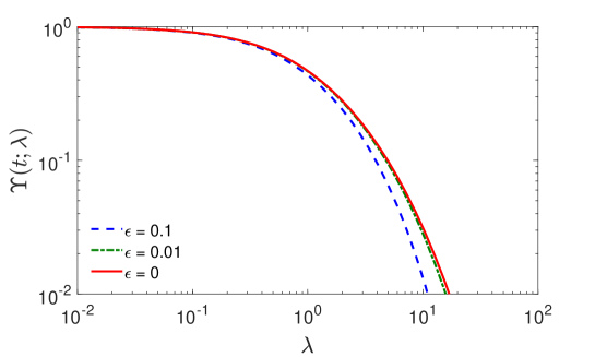
Figure 1: Comparison of the function $\Upsilon(t;\lambda)$ for the Feller diffusing diffusivity model and its approximations by switching diffusion models. Drift and volatility coefficients are set by Eq. (18) with parameters $\bar{D}=1$, $\sigma=1$, $\tau=1$, and $t=1$ (arbitrary units). Solid line shows the explicit solution (20) whereas two other lines present approximate solutions from Eq. (48) for switching diffusion models with ${\epsilon}=0.1$ (dashed line) and ${\epsilon}=0.01$ (dash-dotted line) and $D_{m}=10$.

Left panels of Fig. 2 show the behavior of the function $\Upsilon(t;\lambda)$ for a diffusing diffusivity modeled by reflected Brownian motion on $(0,D_{m})$. Although the exact solution is provided in Sec. 2.2, it is much faster and easier to use the approximate solution via the switching diffusion model. As expected, the function $\Upsilon(t;\lambda)$ approaches $1$ as $t\to 0$ or $\lambda\to 0$. In turn, when either of these variables is getting large, $\Upsilon(t;\lambda)$ decreases. According to Eq. (37), the decay is slow for the case without diffusivity dynamics ($\sigma=0$), see Fig. 2(a). In turn, much faster decay is observed for other cases with $\sigma>0$, in agreement with the asymptotic analysis of Sec. 2.2.

To get a closer look into the behavior of $\Upsilon(t;\lambda)$, it is convenient to plot $-\ln(\Upsilon(t;\lambda))/(t\lambda)$ as a function of $t$. At small $t$, one has $T_{t}\approx D_{0}t$ so that $\Upsilon(t;\lambda)\simeq\langle e^{-t\lambda D_{0}}\rangle\simeq 1-t\lambda\langle D_{0}\rangle$, where $\langle D_{0}\rangle$ is the mean initial diffusivity, which is equal to $D_{m}/2$ in this model. As a consequence, the ratio $-\ln(\Upsilon(t;\lambda))/(t\lambda)$ approaches $D_{m}/2$ as $t\to 0$. The opposite limit $t\to\infty$ is less universal: for instance, Eq. (37) exhibits $\ln(t)/t$ decay, whereas Eq. (31) leads to a constant. Right panels of Fig. 2 illustrate this behavior. All shown curves start from the mean diffusivity $D_{m}/2=0.5$ at $t=0$. As $t$ grows, all curves decrease but the speed of decrease depends on $\lambda$ and $\sigma$. For $\sigma=0$, the ratio vanishes as $t\to\infty$ whereas it reaches a nonzero limit $\sigma^{2}\gamma_{0}(\lambda)/(2\lambda)$ for $\sigma>0$, where $\gamma_{0}(\lambda)$ is the smallest eigenvalue of the operator $\partial^{2}_{D_{0}}-(2\lambda/\sigma^{2})D_{0}$, see Sec. 2.2. As a consequence, this limit changes from $D_{m}/2$ for small $\lambda$ to $|a^{\prime}_{0}|(\sigma^{2}/2)^{1/3}\lambda^{-1/3}$ for large $\lambda$. One can see that the range of variations of $-\ln(\Upsilon(t;\lambda))/(t\lambda)$ is getting narrower as $\sigma$ increases. Indeed, strong fluctuations rapidly mix all diffusivities in $(0,D_{m})$, restoring the behavior with the mean diffusivity $D_{m}/2$, as at short times.

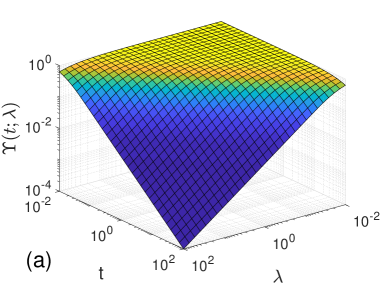
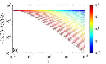
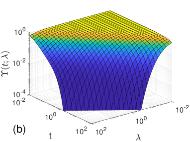
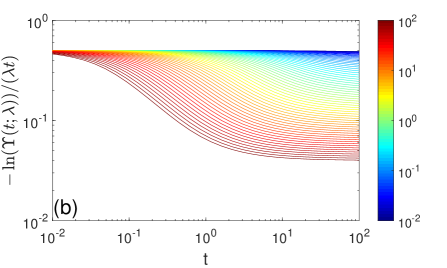
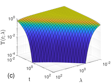
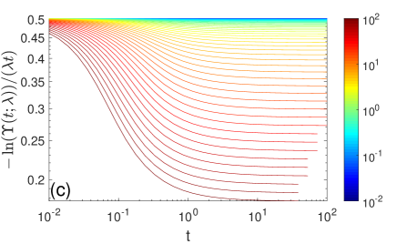
Figure 2: (Left panels) The function $\Upsilon(t;\lambda)$ for the diffusing diffusivity modeled by reflected Brownian motion on $(0,D_{m})$, with $D_{m}=1$ and $\sigma=0$ (a), $\sigma=0.1$ (b), and $\sigma=1$ (c) (arbitrary units). For $\sigma=0$, Eq. (37) was used, whereas for $\sigma>0$, $\Upsilon(t;\lambda)$ was computed from Eq. (48) for an approximate switching diffusion model with ${\epsilon}=0.01$. We checked that a smaller value of ${\epsilon}$ yielded similar results (not shown). The vertical axis is truncated at $10^{-4}$. (Right panels) The ratio $-\ln(\Upsilon(t;\lambda))/(t\lambda)$ as a function of $t$ for the same model and parameters. Each of 64 curves corresponds to a value $\lambda$ sampled between $10^{-2}$ and $10^{2}$ at logarithmic scale (see colorbar).

4 Conclusion

We formulated a unifying approach for studying first-passage time distributions and related diffusion-limited reactions in the realm of diffusing diffusivity and switching diffusion models. In both cases, the dynamics of randomly changing diffusivity $D_{t}$ is assumed to be independent from the particle’s position, so that the subordination argument yields a general spectral expansion for the propagator and the first-passage time probability density. The key element coupling the stochastic diffusivity to the motion of the particle is the moment-generating function $\Upsilon(t;\lambda|D_{0})$ of the integrated diffusivity.

In diffusing diffusivity models, continuous changes of $D_{t}$ are governed by a stochastic differential equation, and the function $\Upsilon(t;\lambda|D_{0})$ can be calculated by using the Feynman-Kac formula. We illustrated this formalism for the case when the diffusivity is modeled by reflected Brownian motion on an interval with reflecting endpoints. In turn, when the diffusivity randomly switches between discrete values, we derived a matrix representation of the function $\Upsilon(t;\lambda|D_{0})$ involving the matrix of switching rates. We also formalized the connection between these two classes of models by relating the coefficients of the stochastic differential equation, $\mu(D)$ and $\sigma(D)$, to the switching rates. With the help of this formalism, one can extend former results on diffusive search problems [2, 5, 32, 56, 57, 58] to heterogeneous diffusion, compute the related first-passage time distributions [3, 59, 60, 61] and investigate diffusion-limited reactions in heterogeneous media.

While continuously changing diffusivity may represent the effect of rapidly re-arranging medium onto the motion of particles, discrete changes of the diffusivity can mimic switching between conformational states of a polymer or reversible binding of the diffusing molecule to other constituents (static or mobile) of the medium. In particular, the state with zero diffusivity can incorporate trapping events. While former studies involving stochastic diffusivity were focused on a specific choice of the Feller process (which includes as a particular case the square of the Ornstein-Uhlenbeck process used in [25, 26, 27]), the general formalism of the present paper opens the door to study a very broad class of various processes in a unified way. As the microscopic theory expressing the impact of rapidly re-arranging media onto the particle’s dynamics in terms of an appropriate diffusing diffusivity model is still missing, the possibility of dealing with a broad range of “candidate processes” is particularly valuable for future research.

References

- [1] Luby-Phelps K 2000 Int. Rev. Cytology 192 189-221
- [2] Loverdo C, Bénichou O, Moreau M, and Voituriez R 2008 Nat. Phys. 4 134-137
- [3] Bénichou O, Chevalier C, Klafter J, Meyer B, and Voituriez R 2010 Nat. Chem. 2 472-477
- [4] Barkai E, Garini Y, and Metzler R 2012 Phys. Today 65 29-35
- [5] Bénichou O and Voituriez R 2014 Phys. Rep. 539 225-284
- [6] He W, Song H, Su Y, Geng L, Ackerson BJ, Peng HB, and Tong P 2016 Nat. Commun. 7 11701
- [7] Bressloff PC and Newby J 2013 Rev. Mod. Phys. 85 135-196
- [8] Höfling F and Franosch T 2013 Rep. Prog. Phys. 76 046602
- [9] Bouchaud J-P and Georges A 1990 Phys. Rep. 195 127
- [10] Metzler R and Klafter J 2000 Phys. Rep. 339 1-77
- [11] Sokolov IM 2012 Soft Matter 8 9043-9052
- [12] Metzler R, Jeon J-H, Cherstvy AG, and Barkai E 2014 Phys. Chem. Chem. Phys. 16 24128-24164
- [13] Guigas G, Kalla C, and Weiss M 2007 Biophys. J. 93 316-323
- [14] Szymanski J and Weiss M 2009 Phys. Rev. Lett. 103 038102
- [15] Weber SC, Spakowitz AJ, and Theriot JA 2010 Phys. Rev. Lett. 104 238102
- [16] Goychuk I Adv. Chem. Phys. 150 187-253
- [17] Bertseva E, Grebenkov DS, Schmidhauser P, Gribkova S, Jeney S, and Forró L 2012 Eur. Phys. J. E 35 63
- [18] Grebenkov DS, Vahabi M, Bertseva E, Forró L, and Jeney S 2013 Phys. Rev. E 88 040701R
- [19] Sadegh S, Higgins JL, Mannion PC, Tamkun MM, and Krapf D 2017 Phys. Rev. X 7 11031
- [20] Manzo C, Torreno-Pina JA, Massignan P, Lapeyre JC Jr., Lewenstein M, and Garcia Parajo MF 2015 Phys. Rev. X 5 011021
- [21] Bénichou O, Loverdo C, Moreau M, and Voituriez R 2011 Rev. Mod. Phys. 83 81-130
- [22] Bressloff PC 2017 J. Phys. A. 50 133001
- [23] Lanoiselée Y, Moutal N, and Grebenkov DS 2018 Nature Commun. 9 4398
- [24] Chubynsky MV and Slater GW 2014 Phys. Rev. Lett. 113 098302
- [25] Jain R and Sebastian KL 2016 J. Phys. Chem. B 120 3988-3992
- [26] Jain R and Sebastian KL 2016 J. Phys. Chem. B 120 9215-9222
- [27] Chechkin AV, Seno F, Metzler R, and Sokolov IM 2017 Phys. Rev. X 7 021002
- [28] Lanoiselée Y and Grebenkov DS 2018 J. Phys. A. 51 145602
- [29] Sposini V, Chechkin AV, Seno F, Pagnini G, and Metzler R 2018 New. J. Phys. 20 043044
- [30] Grebenkov DS and Nguyen B-T 2013 SIAM Rev. 55 601-667
- [31] Gardiner CW 1985 Handbook of Stochastic Methods for Physics, Chemistry and the Natural Sciences (Springer: Berlin).
- [32] Redner S 2001 A Guide to First Passage Processes (Cambridge: Cambridge University press).
- [33] Feller W 1951 Ann. Math. 54 173-182
- [34] Cox JC, Ingersoll JE, and Ross SA 1985 Econometrica 53 385-408
- [35] Sungkaworn T, Jobin M-L, Burnecki K, Weron A, Lohse MJ, and Calebiro D 2017 Nature 550 543-547
- [36] Weron A, Burnecki K, Akin EJ, Solé L, Balcerek M, Tamkun MM, and Krapf D 2017 Scient. Rep. 7 5404
- [37] Yin G and Zhu C 2010 Hybrid Switching Diffusions: Properties and Applications (Springer, New York).
- [38] Godec A and Metzler R 2017 J. Phys. A 50 084001
- [39] Freidlin M 1985 Functional Integration and Partial Differential Equations, Annals of Mathematics Studies (Princeton, New Jersey: Princeton University Press).
- [40] Grebenkov DS 2006 “Partially Reflected Brownian Motion: A Stochastic Approach to Transport Phenomena”, in “Focus on Probability Theory”, Ed. L. R. Velle, pp. 135-169 (Nova Science Publishers).
- [41] Risken H 1996 The Fokker-Planck equation: methods of solution and applications, 3rd Ed. (Berlin: Springer).
- [42] Masoliver J and Perelló J 2012 Phys. Rev. E 86 041116
- [43] Masoliver J 2014 Phys. Rev. E 89 042106
- [44] Gan X and Waxman D 2015 Phys. Rev. E 91 012123
- [45] Stoller SD, Happer W, and Dyson FJ 1991 Phys. Rev. A 44 7459
- [46] Grebenkov DG 2014 J. Magn. Reson. 248 164-176
- [47] Yin G and Zhu C 2010 J. Diff. Eq. 249 2409-2439
- [48] Baran NA, Yin G, and Zhu C 2013 Adv. Diff. Eq. 315
- [49] Bénichou O, Grebenkov DS, Levitz P, Loverdo C, and Voituriez R 2010 Phys. Rev. Lett. 105 150606
- [50] Bénichou O, Grebenkov DS, Levitz P, Loverdo C, and Voituriez R 2011 J. Stat. Phys. 142 657-685
- [51] Rojo F and Budde CE 2011 Phys. Rev. E 84 021117
- [52] Rupprecht J-F, Bénichou O, Grebenkov DS, and Voituriez R 2012 J. Stat. Phys. 147 891-918
- [53] Rupprecht J-F, Bénichou O, Grebenkov DS, and Voituriez R 2012 Phys. Rev. E 86 041135
- [54] Kärger J 1985 Adv. Coll. Int. Sci. 23 129-148
- [55] N. Tyagi and B. J. Cherayil, J. Phys. Chem. B 121, 7204-7209 (2017).
- [56] Metzler R, Oshanin G, and Redner S (Eds.) 2014 First-passage phenomena and their applications (World Scientific Press).
- [57] Holcman D and Schuss Z 2013 Phys. Progr. Rep. 76 074601
- [58] Holcman D and Schuss Z 2014 SIAM Rev. 56 213-257
- [59] Godec A and Metzler R 2016 Sci. Rep. 6 20349
- [60] Grebenkov DS, Metzler R, and Oshanin G 2018 Phys. Chem. Chem. Phys. 20 16393-16401
- [61] Grebenkov DS, Metzler R, and Oshanin G 2018 Commun. Chem. 1 96