Smallest singular value and limit eigenvalue distribution
of a class of non-Hermitian random matrices
with statistical application

Abstract

Suppose $X$ is an $N\times n$ complex matrix whose entries are centered, independent, and identically distributed random variables with variance $1/n$ and whose fourth moment is of order ${\mathcal{O}}(n^{-2})$. In the first part of the paper, we consider the non-Hermitian matrix $XAX^{*}-z$, where $A$ is a deterministic matrix whose smallest and largest singular values are bounded below and above respectively, and $z\neq 0$ is a complex number. Asymptotic probability bounds for the smallest singular value of this matrix are obtained in the large dimensional regime where $N$ and $n$ diverge to infinity at the same rate.

In the second part of the paper, we consider the special case where $A=J=[\mathbbm{1}_{i-j=1\mod n}]$ is a circulant matrix. Using the result of the first part, it is shown that the limit spectral distribution of $XJX^{*}$ exists in the large dimensional regime, and we determine this limit explicitly. A statistical application of this result devoted towards testing the presence of correlations within a multivariate time series is considered. Assuming that $X$ represents a $\mathbb{C}^{N}$-valued time series which is observed over a time window of length $n$, the matrix $XJX^{*}$ represents the one-step sample autocovariance matrix of this time series. Guided by the result on the limit spectral distribution of this matrix, a whiteness test against an MA correlation model for the time series is introduced. Numerical simulations show the excellent performance of this test.

Keywords: Large non Hermitian matrix theory; Limit spectral distribution; Smallest singular value; Whiteness test in multivariate time series.

1 Introduction and the main results

Let $(N^{(n)})_{n\geq 1}$ be a sequence of positive integers, which diverges to $\infty$ as $n\to\infty$. Suppose $(X^{(n)}=[x_{ij}^{(n)}\leavevmode\nobreak\ ]_{i,j=0}^{N^{(n)}-1,n-1})_{n\geq 1}$ is a sequence of complex random matrices whose entries satisfy the following assumptions:

Assumption 1.

For each $n\geq 1$, the complex random variables $\{x_{ij}^{(n)}\}_{i,j=0}^{N^{(n)}-1,n-1}$ are i.i.d. with ${{\mathbb{E}}}x_{00}^{(n)}=0$, ${{\mathbb{E}}}|x_{00}^{(n)}|^{2}=1/n$, and $\sup_{n}n^{2}{{\mathbb{E}}}|x_{00}^{(n)}|^{4}\leq{\boldsymbol{m}}_{4}<\infty$.

Let $(A^{(n)})$ be a sequence of deterministic matrices such that $A^{(n)}\in\mathbb{C}^{n\times n}$, and such that

Assumption 2.

$$0<\inf_{n}s_{n-1}(A^{(n)})\leq\sup_{n}s_{0}(A^{(n)})<\infty\,,$$

where $s_{0}(M)\geq\cdots\geq s_{n-1}(M)$ will refer hereinafter to the singular values of the matrix $M\in\mathbb{C}^{n\times n}$.

Suppose that $N^{(n)}/n\to\gamma$, $0<\gamma<\infty$ as $n\to\infty$. We shall first be interested in the behavior of the smallest singular value of the non-Hermitian matrix $X^{(n)}A^{(n)}{X^{(n)}}^{*}-zI_{N}$, where $z$ is an arbitrary non-zero complex number. We shall then use this result to obtain the limiting spectral behavior of the matrix $X^{(n)}J^{(n)}{X^{(n)}}^{*}$ where $J^{(n)}$ is given by Equation (1) below. Finally, we shall discuss a statistical application of this last result.

The behavior of the smallest singular value of large random matrices has recently aroused an intense research effort in the field of random matrix theory [36]. One of the main motivations for this interest is its close connections with the theory of the spectral behavior of large square non-Hermitian random matrices. It is indeed well-known that the probabilistic control of the smallest singular value of the matrix $Y-z$ is a key step towards understanding the behavior of the spectral measure of the matrix $Y$ [7, 36]. Starting with the fundamental model where $Y$ has i.i.d. elements, most of the contributions dealing with the smallest singular value assume the independence between the entries of $Y$, as seen in [25, 33, 16, 37, 9] among many others. More structured models, such as the one dealt with in this paper, have received comparatively much less attention.

Our results will be established under the following additional assumption on the elements of $X^{(n)}$.

Assumption 3.

The random variables $x_{00}^{(n)}$ satisfy $\sup_{n}|n{{\mathbb{E}}}(x_{00}^{(n)})^{2}|<1$.

To understand the implication of Assumption 3, suppose it does not hold. Drop the superscript ⁽ⁿ⁾, and write $x_{00}=\Re x_{00}+\imath\Im x_{00}$. In that case, $1/n=|{{\mathbb{E}}}x_{00}^{2}|={{\mathbb{E}}}|x_{00}|^{2}$. Expanding the expectations, this implies that $({{\mathbb{E}}}\Re x_{00}\Im x_{00})^{2}={{\mathbb{E}}}(\Re x_{00})^{2}{{\mathbb{E}}}(\Im x_{00})^{2}$. Suppose for the moment, $\Re x_{00}\not\equiv 0$. Then clearly $\Im x_{00}=\alpha\Re x_{00}$ w.p.1 for some constant $\alpha$. Thus, $x_{00}\stackrel{{\scriptstyle{\mathcal{L}}}}{{=}}\exp(\imath\theta)Z$, where $Z$ is a real random variable and $\theta$ is a constant. This amounts to $x_{00}$ being real since the factor $\exp(\imath\theta)$ has no influence on $XJX^{*}$. Thus, Assumption 3 essentially says that the $x_{ij}$ are not real.

We can now state our first result. We denote as $\|\cdot\|$ the spectral norm of a matrix. Events are expressed in the forms $[\ldots]$ or $\{\ldots\}$.

Theorem 1.

Let Assumptions 1, 2, and 3 hold true. Then, there exist $\alpha,\beta>0$ such that for each $C>0$, $t>0$, and $z\in\mathbb{C}\setminus\{0\}$,

$${{\mathbb{P}}}\left[s_{N-1}(X^{(n)}A^{(n)}{X^{(n)}}^{*}-z)\leq t,\ \|X\|\leq C\right]\leq c\left(n^{\alpha}t^{1/2}+n^{-\beta}\right),$$

where the constant $c>0$ depends on $C$, $z$, and ${\boldsymbol{m}}_{4}$ only.

To prove this theorem, the first step is to linearize the model $X^{(n)}A^{(n)}{X^{(n)}}^{*}-z$ by considering the matrix

$$H^{(n)}=\begin{bmatrix}{A^{(n)}}^{-1}&{X^{(n)}}^{*}\\ X^{(n)}&z\end{bmatrix}\in\mathbb{C}^{(N+n)\times(N+n)}.$$

By using, e.g., the inversion formula for partitioned matrices, it is easy to see that

$$\|(X^{(n)}A^{(n)}{X^{(n)}}^{*}-z)^{-1}\|\leq\|{H^{(n)}}^{-1}\|$$

(versions of this “linearization trick” have been used in many different contexts, see, e.g., [19]). Thus, the problem is reduced to controlling the smallest singular value of $H^{(n)}$. A similar problem was tackled in [40] and [28]. In this paper, we follow closely the approach of  [40]. However, there instead of $H^{(n)}$, the author had a real symmetric matrix with i.i.d. elements above the diagonal. Our matrix $H^{(n)}$ is more structured, and this necessitates a suitable modification in the arguments. Theorem 1 will be proven in Section 3.

Theorem 1 can be used to study the eigenvalue distribution of the matrix $X^{(n)}A^{(n)}{X^{(n)}}^{*}$ in the large dimensional regime (see [7] or Section 4 below for more explanations on this connection). Motivated by the statistical application described in Section 2, we shall restrict our study in this paper to the specific case where $A^{(n)}$ equals the circulant matrix

$$J^{(n)}=\begin{bmatrix}0&&&1\\ 1&\ddots&\\ &\ddots&\ddots\\ &&1&0\end{bmatrix}\in{{\mathbb{R}}}^{n\times n},$$ (1)

This matrix satisfies Assumption 2, since it is orthogonal. Let $\{\lambda_{0}^{(n)},\ldots,\lambda_{N^{(n)}-1}^{(n)}\}$ be the eigenvalues of the matrix $X^{(n)}J^{(n)}{X^{(n)}}^{*}$, which are in general complex-valued. The spectral distribution or measure of this matrix is defined as the random probability measure:

$$\mu_{n}=\frac{1}{N^{(n)}}\sum_{i=0}^{N^{(n)}-1}\delta_{\lambda_{i}^{(n)}}.$$

Given a sequence of random probability measures $(\zeta_{n})$ on the space ${\mathcal{X}}={{\mathbb{R}}}$ or $\mathbb{C}$ and a deterministic probability measure $\boldsymbol{\zeta}$ on ${\mathcal{X}}$, we recall that $\zeta_{n}$ is said to converge weakly in the almost sure sense (resp. in probability) if for each continuous and bounded real function $\varphi$ on ${\mathcal{X}}$,

$$\int\varphi\,d\zeta_{n}\xrightarrow[n\to\infty]{}\int\varphi\,d{\boldsymbol{\zeta}}\quad\text{almost surely (resp. in probability).}$$

This weak convergence will be denoted as $\zeta_{n}\Rightarrow\boldsymbol{\zeta}$ a.s. (resp. in probability).

In the asymptotic regime where $N^{(n)}/n\to\gamma$, $0<\gamma<\infty$, we shall identify a deterministic probability measure $\boldsymbol{\mu}$ such that $\mu_{n}\Rightarrow\boldsymbol{\mu}$ in probability. This limit $\boldsymbol{\mu}$ is called the limiting spectral distribution or measure (LSD) of the sequence of matrices. To state our result regarding this LSD, we need the following function. For any $0<\gamma<\infty$, let

$$g(y)=\frac{y}{y+1}(1-\gamma+2y)^{2},\ (0\vee(\gamma-1))\leq y\leq\gamma.$$ (2)

Then $g^{-1}$ exists on the interval $[0\vee((\gamma-1)^{3}/\gamma),\gamma(\gamma+1)]$ and maps it to $[0\vee(\gamma-\gamma^{-1}),\gamma]$. It is an analytic increasing function on the interior of the interval.

Theorem 2.

Suppose Assumptions 1 and 3 hold. Then, there exists a deterministic probability measure $\boldsymbol{\mu}$ such that $\mu_{n}\Rightarrow\boldsymbol{\mu}$ in probability. The limit measure $\boldsymbol{\mu}$ is rotationally invariant on $\mathbb{C}$. Let $F(r)=\boldsymbol{\mu}(\{z\in\mathbb{C}\,:\,|z|\leq r\}),\ 0\leq r<\infty$ be the distribution function of the radial component.

If $\gamma\leq 1$, then

$$F(r)=\left\{\begin{array}[]{cl}\gamma^{-1}g^{-1}(r^{2})&\text{if}\ 0\leq r\leq\sqrt{\gamma(\gamma+1)},\\ \\ 1&\text{if}\ r>\sqrt{\gamma(\gamma+1)}.\end{array}\right.$$

If $\gamma>1$, then

$$F(r)=\left\{\begin{array}[]{cl}1-\gamma^{-1}&\text{if}\ 0\leq r\leq(\gamma-1)^{3/2}/\sqrt{\gamma},\\ \\ \gamma^{-1}g^{-1}(r^{2})&\text{if}\ (\gamma-1)^{3/2}/\sqrt{\gamma}<r\leq\sqrt{\gamma(\gamma+1)},\\ \\ 1&\text{if}\ r>\sqrt{\gamma(\gamma+1)}.\end{array}\right.$$

The theorem implies that the support of $\boldsymbol{\mu}$ is the disc $\{z:|z|\leq\sqrt{\gamma(\gamma+1)}\}$ when $\gamma\leq 1$, and when $\gamma>1$, it is the ring $\{z:(\gamma-1)^{3/2}/\sqrt{\gamma}\leq|z|\leq\sqrt{\gamma(\gamma+1)}\}$ together with the point $\{0\}$ where there is a mass $1-\gamma^{-1}$.

Moreover, $F(r)$ has a positive and analytical density on the open interval $(0\vee\operatorname{sign}(\gamma-1)|\gamma-1|^{3/2}/\sqrt{\gamma},\sqrt{\gamma(\gamma+1)})$. A closer inspection of $g$ shows that this density is bounded if $\gamma\neq 1$. If $\gamma=1$, then the density is bounded everywhere except when $r\downarrow 0$. A cumbersome closed form expression for $g^{-1}$ (and hence for $F(\cdot)$) can be obtained by calculating the root of a third degree polynomial. For the special case $\gamma=1$, $g^{-1}$ is given by

$$g^{-1}(t)=\frac{t^{1/3}}{2}\left(\left[1+\sqrt{1-\frac{t}{27}}\right]^{1/3}+\left[1-\sqrt{1-\frac{t}{27}}\right]^{1/3}\right),\quad 0\leq t\leq 2.$$

As an illustration of these results, eigenvalue realizations corresponding to the cases where $\gamma=0.5$ and $\gamma=2$ are shown in Figure 1. Plots of the functions $F(r)$ given in the statement of Theorem 2 are shown on Figure 2, along with their empirical counterparts.

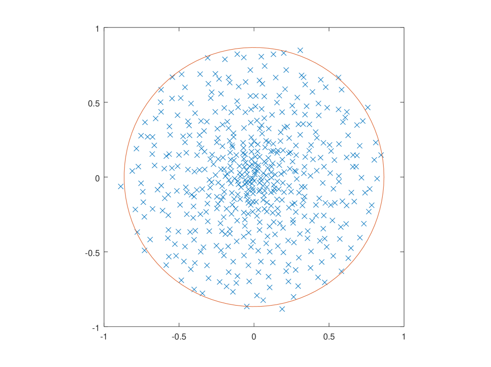
(a) $(N,n)=(500,1000)$

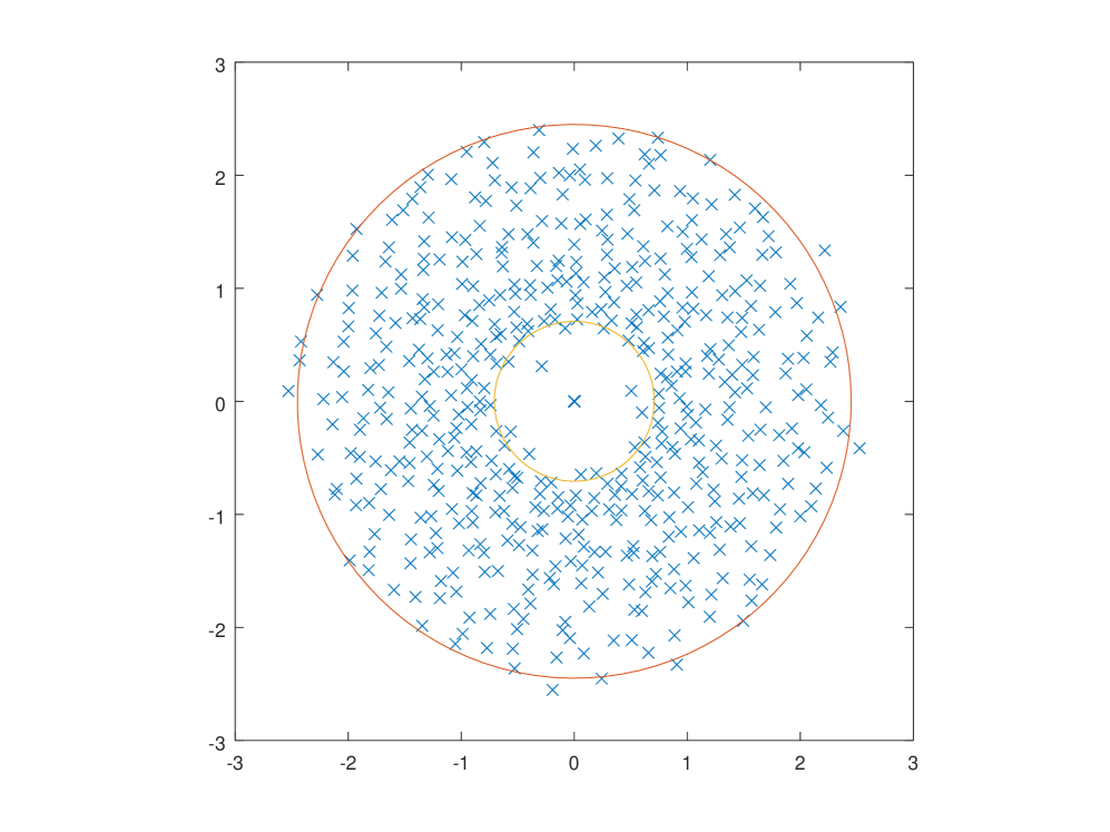
(b) $(N,n)=(1000,500)$

Figure 1: Eigenvalue realizations and LSD support.

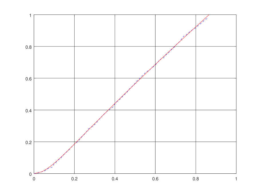
(a) $(N,n)=(500,1000)$

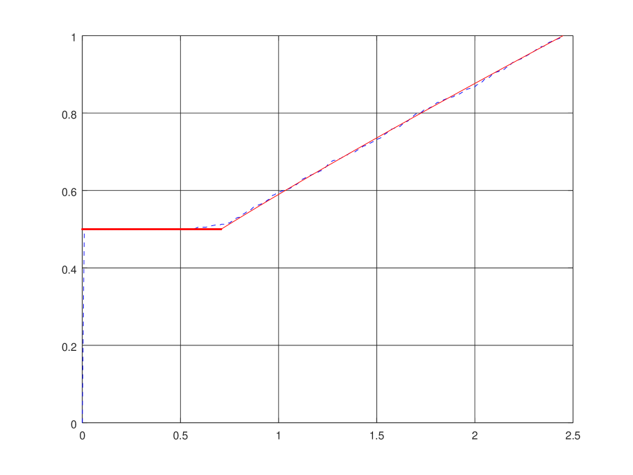
(b) $(N,n)=(1000,500)$

Figure 2: Plots of $F(r)$ (plain curves) and their empirical realizations (dashed curves).

Theorem 2 is proven in Sections 4 – 6. Before turning to the proofs of Theorems 1 and 2, we consider in the next section a statistical application of these results.

2 Application to statistical hypothesis testing

Consider the high dimensional linear moving average time series model

$$y_{t}^{(n)}=\sum_{i=0}^{p}B_{i}^{(n)}w_{t-i}^{(n)},$$ (3)

where $\{B_{i}^{(n)}\}_{i=0}^{p}$ are $\mathbb{C}^{N\times N}$ deterministic parameter matrices, and $\{w_{i}^{(n)}\}_{i}$ are random vectors such that the random matrix $W^{(n)}=[w_{0}^{(n)}\ \cdots\ w_{n-1}^{(n)}]$ is equal in distribution to $n^{1/2}X^{(n)}$. Such models have found increasing attention in, e.g., the fields of signal processing, wireless communications, Radar, Sonar, and wideband antenna array processing [20, 39]. The sample autocovariance matrices $\{n^{-1}\sum_{t=k+1}^{n}y_{t}^{(n)}(y_{t-k}^{(n)})^{*}\},k\geq 0$, ($k$ is called the lag or the step) carry useful information about the model (3), specially through their spectral distributions. Some of the works that deal with limit spectral distributions, mostly for high-dimensional real-valued time series, and their use in statistical inference are, [2, 3, 4, 5, 26, 41, 24, 23, 6].

The $k$-step sample autocovariance matrices, except for the order $k=0$, are non-Hermitian. LSD results are so far known only for certain symmetrized versions of these matrices. All the references cited above rely on this idea of symmetrization. To the best of our knowledge, no LSD results are known for the non-Hermitian sample autocovariance matrices. The result of Theorem 2 above is a beginning towards deriving the LSD of the sample autocovariance matrices in the general model (3) by considering the simplest case where $B_{0}^{(n)}=I_{N}$ and $p=0$. This will be called the white noise model.

Consider the problem of testing the white noise model against an MA correlated model. To this end, we explore the idea of designing a test which is based on the eigenvalue distribution of the one-step sample autocovariance matrix, in contrast to more classical tests that are based on its singular value distribution. A non-rigorous justification of this idea is that when performing an eigenvalue-based test, we take advantage of the higher sensitivity of the eigenvalues of a matrix with respect to perturbations as compared to its singular values.

Assuming for simplicity that $p=1$, our purpose is to test the null (white noise) hypothesis H0: $B_{0}^{(n)}=I,B_{1}^{(n)}=0$ against the alternative H1: $B_{0}^{(n)}=I,B_{1}^{(n)}\neq 0$. Consider the one-step sample autocovariance matrix

$$\widehat{R}_{1}^{(n)}=\frac{1}{n}\sum_{t=0}^{n-1}y_{t}^{(n)}{y_{t-1}^{(n)}}^{*},$$

where the sum is taken modulo $n$, and observe that under H0, this matrix coincides with $X^{(n)}J^{(n)}{X^{(n)}}^{*}$. We shall consider the asymptotic regime where $n\to\infty$ and $N/n\to\gamma>0$. By Theorem 2, the spectral measure of $\widehat{R}_{1}^{(n)}$ converges weakly in probability to the measure $\boldsymbol{\mu}$. This suggests the use of a white noise test based on a distance between the spectral measure of $\widehat{R}_{1}^{(n)}$ and $\boldsymbol{\mu}$. We consider herein a test based on the $2$-Wasserstein distance between these two distributions. For the sake of comparison, we also considered the more classical singular value based test which consists in comparing $N^{-1}\operatorname{tr}\widehat{R}_{1}^{(n)}(\widehat{R}_{1}^{(n)})^{*}$ to a threshold. We denote these two tests as T1 and T2 respectively.

To get a more complete picture of the problem, we also considered a third test which is based on the eigenvalue distribution of the Hermitian sample covariance matrix

$$\widehat{R}_{0,1}^{(n)}=\frac{1}{n}\sum_{t=0}^{n-1}\begin{bmatrix}y_{t}^{(n)}\\ y_{t-1}^{(n)}\leavevmode\nobreak\ \end{bmatrix}\begin{bmatrix}{y_{t}^{(n)}}^{*}&{y_{t-1}^{(n)}}^{*}\leavevmode\nobreak\ \end{bmatrix}.$$

Its spectral distribution is known to converge weakly almost surely under H0 to the Marchenko-Pastur distribution $\text{MP}_{2\gamma}$ with parameter $2\gamma$ (see [27], which deals with the Gaussian case). This suggests the use of the $2$-Wasserstein distance between the spectral measure of $\widehat{R}_{0,1}$ and $\text{MP}_{2\gamma}$. We denote the resulting test as T3.

Figures 3 and 4 represent the ROC curves obtained for these three tests. The tests T1 and T3 were implemented by sampling $\boldsymbol{\mu}$ and $\text{MP}_{2\gamma}$ from the spectra of two large random matrices and by using the transport library of the R software. For Figure 3, $B_{1}^{(n)}=\alpha I_{N}$, while for Figure 4, the elements $b_{ij}$ of $B_{1}^{(n)}$ are chosen as $b_{ij}=\alpha^{\prime}\exp(-8|i-j|/N)$, where $\alpha$ and $\alpha^{\prime}$ are non-zero real numbers.

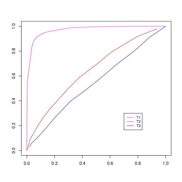
Figure 3: ROC curves. Setting: $B_{1}^{(n)}=\alpha I_{N}$ with $\alpha^{2}=10^{-2.5}$, $(N,n)=(50,100)$.

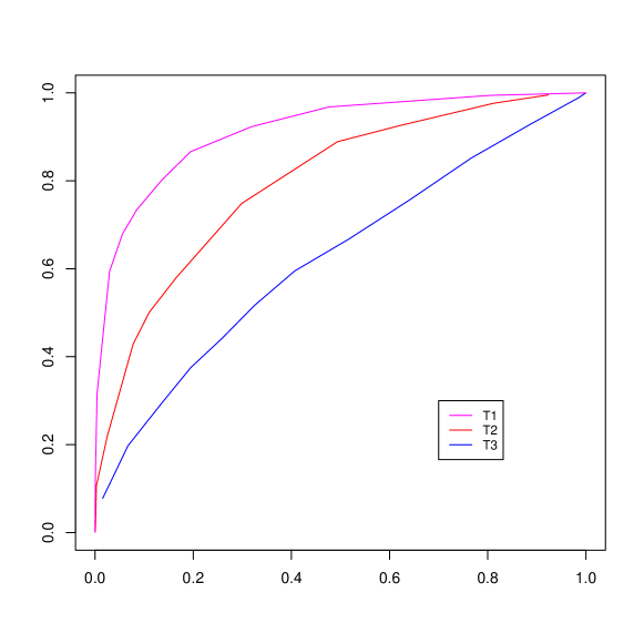
Figure 4: ROC curves. Setting: $B_{1}^{(n)}$ is a Toeplitz matrix with $\operatorname{tr}B_{1}^{(n)}(B_{1}^{(n)})^{*}/N=10^{-2}$, $(N,n)=(50,100)$.

These figures clearly show that T1 outperforms T2 and T3. This tends to corroborate the intuition that the eigenvalue sensitivity alluded to earlier, can be beneficial when it comes to designing white noise tests.

To better understand the behavior of the eigenvalue-based tests, the next step would be to study the large dimensional behavior of the spectral distribution of $\widehat{R}_{1}^{(n)}$ under H1. This appears to be quite non-trivial and is left for future research.

Notations

The notations $\dim(V)$ and $V^{\perp}$ will refer to the dimension of the vector subspace $V$, and the subspace orthogonal to $V$ respectively. The column span of a matrix $M$ will be denoted as $\operatorname{span}(M)$. Similarly, $\operatorname{span}(V,d)$ is the span of the vector space $V$ and the vector $d$.

The indices of the elements of a vector or a matrix start from zero. Given a positive integer $m$, we write $[m]=\{0,\ldots,m-1\}$. For $i\in[m]$, we denote as $e_{m,i}$ the $i^{\text{th}}$ canonical vector of $\mathbb{C}^{m}$, with $1$ at the $m$th place and $0$ elsewhere. Given a matrix $M\in\mathbb{C}^{m\times n}$ and two sets ${\mathcal{I}}\subset[m]$ and ${\mathcal{J}}\subset[n]$, we denote as $M_{{\mathcal{I}},{\mathcal{J}}}$ the $|{\mathcal{I}}|\leavevmode\nobreak\ \times|{\mathcal{J}}|$ submatrix of $M$ that is obtained by retaining the rows of $M$ whose indices belong to ${\mathcal{I}}$ and the columns whose indices belong to ${\mathcal{J}}$. We also write $M_{\cdot,k}=M_{[m],\{k\}}$ and $M_{k,\cdot}=M_{\{k\},[n]}$. We define as $\Pi_{\mathcal{I}}:\mathbb{C}^{m}\to\mathbb{C}^{m}$ the projection operator such that $\Pi_{\mathcal{I}}u$ is the vector obtained by setting to zero the elements of $u$ whose indices are in ${\mathcal{I}}^{\text{c}}$. We also denote as $u_{\mathcal{I}}$ the vector of $\mathbb{C}^{|{\mathcal{I}}|}$ obtained by removing the elements of $u$ whose indices are in ${\mathcal{I}}^{\text{c}}$. When $M$ is a matrix, $\Pi_{M}$ refers to the orthogonal projector on $\operatorname{span}(M)$.

As mentioned above, $\|\cdot\|$ denotes the spectral norm. It will also denote the Euclidean norm of a vector. The Hilbert-Schmidt norm of a matrix will be denoted as $\|\cdot\|_{\text{HS}}$. The unit-sphere of $\mathbb{C}^{n}$ will be denoted as ${{\mathbb{S}}}^{n-1}$.

The notations ${{\mathbb{P}}}_{x}$ and ${{\mathbb{E}}}_{x}$ will refer respectively to the probability and the expectation with respect to the law of the vector $x$.

3 Proof of Theorem 1: smallest singular value

To simplify the notations, from now on, we omit the superscript ⁽ⁿ⁾. We shall mostly work on the matrix $A^{-1}$ instead of working on $A$. Writing ${\bf s}_{\text{inf}}=\inf_{n}s_{n-1}(A^{-1})$ and ${\bf s}_{\text{sup}}=\sup_{n}s_{0}(A^{-1})$, Assumption 2 is rewritten as $0<{\bf s}_{\text{inf}}\leq{\bf s}_{\text{sup}}<\infty$. We also assume that $z\neq 0$ without further mention.

3.1 General context and outline of proof

We first observe that if we establish Theorem 1 under the assumption that the entries have densities, then it continues to hold in the general case. This is because we can replace the matrix $X$ with, say, the independent sum $(1-n^{-20})^{-1/2}(X+n^{-10}X^{\prime})$ where $X^{\prime}$ is a properly chosen matrix whose elements have densities, and use a standard perturbation argument. Hence, we assume throughout this section that the elements of $X$ have densities. It may be noted that instead of 20, any other positive number could be used and that would sharpen some of the bounds obtained later. However, it was not our goal to achieve sharp bounds.

Suppose $E\in\mathbb{C}^{N\times n}$ is such that $\|E\|^{2}\|A\|<|z|$. Then $\det(z-EAE^{*})\neq 0$. This implies that the multivariate polynomial $\det(z-XAX^{*})$ in the variables $(\Re x_{ij},\Im x_{ij})_{i,j}$ is not identically zero. Since $X$ has a density, we conclude that $z-XAX^{*}$ is invertible w.p. 1.

Define the matrix

$$H=\begin{bmatrix}A^{-1}&X^{*}\\ X&z\end{bmatrix}\in\mathbb{C}^{(N+n)\times(N+n)}.$$

By the well-known inversion formula for partitioned matrices [21, §0.7.3], we have

$$H^{-1}=\begin{bmatrix}A+AX^{*}(z-XAX^{*})^{-1}XA&-AX^{*}(z-XAX^{*})^{-1}\\ -(z-XAX^{*})^{-1}XA&(z-XAX^{*})^{-1}\end{bmatrix},$$

which shows that

$$\|(XAX^{*}-z)^{-1}\|\leq\|H^{-1}\|.$$

Therefore, to obtain Theorem 1, it is enough to prove that

$${{\mathbb{P}}}\left[s_{N+n-1}(H)\leq t,\ \|X\|\leq C\right]\leq c\left(n^{\alpha}t^{1/2}+n^{-\beta}\right),$$ (4)

where $c>0$ depends on $C$, $z$, and ${\boldsymbol{m}}_{4}$ only.

As we mentioned in the introduction, a similar problem was considered in [40] and [28]. We shall follow here the argument of [40]. However, since our matrix $H$ is more structured than the one considered in this reference, a substantial adaptation of the proof is required. Here is a description of the general approach.

First recall that

$$s_{N+n-1}(H)=\min_{u\in{{\mathbb{S}}}^{N+n-1}}\|Hu\|.$$

Invoking an idea that has been frequently used in the literature since [25, 33], we partition ${{\mathbb{S}}}^{N+n-1}$ into two sets of compressible and incompressible vectors as follows.

Let $\theta,\rho\in(0,1)$ be fixed. A vector in ${{\mathbb{S}}}^{N+n-1}$ is said to be $\theta$-sparse if it does not have more than $\lfloor\theta(N+n)\rfloor$ non-zero elements. Let ${{\mathbb{S}}}^{N+n-1}_{\mathcal{I}}$ be the set of vectors of ${{\mathbb{S}}}^{N+n-1}$ that are supported by the (index) set ${\mathcal{I}}\subset[N+n]$. Given $S\subset\mathbb{C}^{N+n}$, let ${\mathcal{N}}_{\delta}(S)$ denote the $\delta$-neighborhood of $S$ in $\mathbb{C}^{N+n}$ in the Euclidean metric.

Given $\theta,\rho\in(0,1)$, we define the set of $(\theta,\rho)$-compressible vectors as

$$\text{comp}(\theta,\rho)={{\mathbb{S}}}^{N+n-1}\cap\bigcup_{\begin{subarray}{c}{\mathcal{I}}\subset[N+n]\leavevmode\nobreak\ \\ |{\mathcal{I}}|=\lfloor\theta(N+n)\rfloor\end{subarray}}{\mathcal{N}}_{\delta}({{\mathbb{S}}}_{{\mathcal{I}}}^{N+n-1}).$$

Note that this is the set of all unit vectors at a distance less or equal to $\rho$ from the set of the $\theta$-sparse unit vectors. The set $\text{incomp}(\theta,\rho)$ of $(\theta,\rho)$-incompressible vectors is the complementary set ${{\mathbb{S}}}^{N+n-1}\setminus\text{comp}(\theta,\rho)$.

With these notations, we write

$$s_{N+n-1}(H)=\inf_{u\in\text{comp}(\theta,\rho)}\|Hu\|\ \wedge\ \inf_{u\in\text{incomp}(\theta,\rho)}\|Hu\|$$ (5)

for judiciously chosen $\theta,\rho\in(0,1)$.

The infimum over $\text{comp}(\theta,\rho)$ is relatively easier to handle. Given a fixed vector $u\in{{\mathbb{S}}}^{N+n-1}$, we first show that ${{\mathbb{P}}}\left[\|Hu\|\leq c\right]$ for some $c>0$ is exponentially small in $n$. Recall that an $\varepsilon$-net is a set of points that are separated from each other by a distance of at most $\varepsilon$. Now, since the vectors of $\text{comp}(\theta,\rho)$ are close to being sparse, it has an $\varepsilon$-net of controlled cardinality for a well-chosen $\varepsilon>0$. Using this, along with a simple union bound, we will be able to infer the smallness of the probability that $\inf_{u\in\text{comp}(\theta,\rho)}\|Hu\|$ is small.

The infimum over the set of incompressible vectors poses a much bigger challenge since the $\varepsilon$-net argument fails. In this case the argument is more geometric. Observe that when $u$ is incompressible, $Hu$ is close to a sum of ${\mathcal{O}}(n)$ columns of $H$ with comparable weights. This helps to reduce the problem of controlling $\inf_{u\in\text{incomp}(\theta,\rho)}\|Hu\|$ to the problem of controlling the distance between an arbitrary column of $H$ and the subspace generated by the other columns.

Let $h_{0}$ be the first column of $H$, and let $H_{-0}\in\mathbb{C}^{(N+n)\times(N+n-1)}$ be the submatrix left after extracting this column. Partition $H$ accordingly as

$$H=\begin{bmatrix}b&g_{01}\\ g_{10}&G\end{bmatrix},$$

with $b\in\mathbb{C}$ and $G\in\mathbb{C}^{(N+n-1)\times(N+n-1)}$. Then, the distance $\operatorname{dist}(h_{0},H_{-0})$ between $h_{0}$ and the column span of $H_{-0}$ equals ($G^{-1}$ will be shown to exist)

$$\operatorname{dist}(h_{0},H_{-0})=\frac{\left|b-g_{01}G^{-1}g_{10}\leavevmode\nobreak\ \right|}{\sqrt{1+\|g_{01}G^{-1}\|^{2}}}.$$ (6)

Our purpose is to bound the probability that this distance is small. If we write

$$A^{-1}=\begin{bmatrix}b&b_{01}\\ b_{10}&B\end{bmatrix},\quad X=\begin{bmatrix}x&W\end{bmatrix},$$

where $B\in\mathbb{C}^{(n-1)\times(n-1)}$, and $x\in\mathbb{C}^{N}$ is the first column of $X$, then

$$g_{01}=\begin{bmatrix}b_{01}&x^{*}\end{bmatrix},\ g_{10}=\begin{bmatrix}b_{10}\\ x\end{bmatrix},\ \text{and}\ G=\begin{bmatrix}B&W^{*}\\ W&zI_{N}\end{bmatrix}.$$ (7)

Assuming inverse exists, partition $G^{-1}$ as

$$G^{-1}=\begin{bmatrix}E&F\\ P&R\end{bmatrix},\quad E\in\mathbb{C}^{(n-1)\times(n-1)},\ R\in\mathbb{C}^{N\times N}.$$ (8)

Then using Equation (6), we have

$$\operatorname{dist}(h_{0},H_{-0})=\frac{\text{Num}}{\text{Den}},$$ (9)

where

$$\begin{split}\text{Num}&=\left|b-b_{01}Eb_{10}-x^{*}Pb_{10}-b_{01}Fx-x^{*}Rx\right|,\quad\text{and}\\ \text{Den}&=\left(1+\|b_{01}E+x^{*}P\|^{2}+\|b_{01}F+x^{*}R\|^{2}\right)^{1/2}.\end{split}$$ (10)

To control the behavior of Num, we need an anti-concentration result. Loosely speaking, we show that conditionally on the matrix $W$ and for most of these matrices, the probability that a properly normalized version of the random variable $x^{*}Pb_{10}+b_{01}Fx+x^{*}Rx$ lives in an arbitrary ball of $\mathbb{C}$ of small radius is itself small.

Small ball probabilities are captured by the so-called Lévy’s concentration function. Given a constant vector $a\in\mathbb{C}^{n}$ and a random vector $Z\in\mathbb{C}^{n}$, Lévy’s concentration function of the inner product $\langle a,Z\rangle$ at $\varepsilon>0$ is

$${\mathcal{L}}_{Z}(\langle a,Z\rangle,\varepsilon)=\sup_{w\in\mathbb{C}}{{\mathbb{P}}}_{Z}\left[\left|\langle a,Z\rangle-w\right|\leq\varepsilon\right].$$

When the elements of $Z$ are i.i.d. random variables with finite third moment, the behavior of ${\mathcal{L}}_{Z}$ can be controlled by the Berry-Esséen theorem, whose use in random matrix theory dates back to [25]. Berry-Esséen theorem is a refinement of the Central Limit Theorem and implies that when $a\in{{\mathbb{S}}}^{n-1}$ has ${\mathcal{O}}(n)$ elements with magnitudes of order $1/\sqrt{n}$, it holds that ${\mathcal{L}}_{Z}(\langle a,Z\rangle,\varepsilon)\lesssim\varepsilon+1/\sqrt{n}$.

Our plan now is to apply this theorem after replacing $Z$ with the random vector $x$. Unfortunately, this theorem cannot be used as is on the random variable $x^{*}Pb_{10}+b_{01}Fx+x^{*}Rx$ because of the presence of the quadratic form $x^{*}Rx$. To circumvent this problem, we use a decoupling argument that replaces $x^{*}Pb_{10}+b_{01}Fx+x^{*}Rx$ with an inner product that can be processed by the Berry-Esséen theorem. This decoupling idea that dates back to [15] has also been used in [40].

3.2 Technical results

The following proposition is a variation of [37, Prop. 5.1], see also [7, Lem. A2] and [17]. This variation is needed because we want the constants $c$ and $c^{\prime}$ to depend on the law of the $Z_{i}$’s via $\kappa$ and $C_{\kappa}$. For completeness, we provide the modified proof in Appendix A.1.

Proposition 3 (Distance of a random vector to a constant subspace).

Let $Z=(Z_{0},\ldots,Z_{n-1})\in\mathbb{C}^{n}$ be a vector of i.i.d. centered unit-variance random variables such that for some $\kappa>0$, ${{\mathbb{E}}}|Z_{0}|^{2+\kappa}\leq C_{\kappa}<\infty$. Then, there exist $c,c^{\prime}>0$ and $\delta\in(0,1)$ that depend only on $\kappa$ and $C_{\kappa}$ and that satisfy the following property. For all $n\gg 1$, and for any deterministic subspace $V$ of $\mathbb{C}^{n}$ such that $0\leq\dim(V)\leq\delta n$,

$${{\mathbb{P}}}[\operatorname{dist}(Z,V)\leq c\sqrt{n}]\leq\exp(-c^{\prime}n).$$

We shall also make use of:

Lemma 4 (Rosenthal’s inequality [32]).

Let $Z_{0},\ldots,Z_{n-1}$ be independent random variables such that ${{\mathbb{E}}}Z_{i}=0$ and ${{\mathbb{E}}}|Z_{i}|^{p}<\infty$ for $p>2$. Then there exists a universal constant $C_{p}$ such that

$${{\mathbb{E}}}\Bigl{|}\sum_{i=0}^{n-1}Z_{i}\Bigr{|}^{p}\leq C_{p}\Bigl{(}\sum_{i=0}^{n-1}{{\mathbb{E}}}|Z_{i}|^{p}\ \vee\ \Bigl{(}\sum_{i=0}^{n-1}{{\mathbb{E}}}|Z_{i}|^{2}\Bigr{)}^{p/2}\Bigr{)}.$$

These results easily lead to the following lemma:

Lemma 5.

Let the matrix $X$ satisfy Assumption 1. Then, there exist constants $c,c^{\prime}>0$ and a constant $\delta\in(0,1)$ that depend on ${\boldsymbol{m}}_{4}$ only and that satisfy the following property. For each deterministic vector $u\in{{\mathbb{S}}}^{n-1}$ and each deterministic subspace $V\subset\mathbb{C}^{N}$ with $0\leq\dim(V)\leq\delta N$,

$${{\mathbb{P}}}\left[\operatorname{dist}(Xu,V)\leq c\right]\leavevmode\nobreak\ \leq\exp(-c^{\prime}n).$$ (11)

In particular, for each deterministic vector $a\in\mathbb{C}^{N}$, it holds that ${{\mathbb{P}}}\left[\|Xu-a\|\leq c\right]\leavevmode\nobreak\ \leq\exp(-c^{\prime}n)$. Similar conclusions hold if $X$ is replaced with $X^{*}$.

Proof.

Let $\tilde{x}_{0},\ldots,\tilde{x}_{N-1}\in\mathbb{C}^{1\times n}$ be the rows of $X$, and define the random variables $Z_{k}=\sqrt{n}\tilde{x}_{k}u$ for $k\in[n]$. These random variables are i.i.d., centered, and have unit-variance. Furthermore, writing $u=[u_{0},\ldots,u_{n-1}]^{\mathsf{T}}$, we get by Rosenthal’s inequality that for some universal constant $C$,

$${{\mathbb{E}}}|Z_{1}|^{4}\leq C\left((n^{2}{{\mathbb{E}}}|X_{11}|^{4}\sum|u_{i}|^{4})\ \vee\ 1\right)\leq C{\boldsymbol{m}}_{4}.$$

Writing $Z=[Z_{0},\ldots,Z_{N-1}]^{\mathsf{T}}$, we note that $\operatorname{dist}(Xu,V)=\operatorname{dist}(Z,V)/\sqrt{n}$. Applying Proposition 3 with $\kappa=2$, we obtain (11). The rest of the claims follow immediately. ∎

The $\varepsilon$-net argument alluded to above will use the following lemma.

Lemma 6 (Metric entropy of a complex sphere, Lemma 2.2 of [9]).

Let $V\in\mathbb{C}^{n}$ be a $k$-dimensional subspace, and let $S\subset V$. Given $\varepsilon>0$, the set ${{\mathbb{S}}}^{n-1}\cap S$ has an $\varepsilon$-net of cardinality bounded by $(3/\varepsilon)^{2k}$.

The two following results regarding Lévy’s concentration functions will be needed.

Lemma 7 (Restriction of the concentration function, Lemma 2.1 of [33]).

Let $Z\in\mathbb{C}^{n}$ be a vector of independent random variables. Then, for each non-empty ${\mathcal{I}}\subset[n]$, we have ${\mathcal{L}}_{Z}(\langle a,Z\rangle,\varepsilon)\leq{\mathcal{L}}_{Z_{\mathcal{I}}}(\langle a_{{\mathcal{I}}},Z_{\mathcal{I}}\rangle,\varepsilon)$.

Proposition 8 (Anti-concentration via the Berry-Esséen theorem).

There exists a constant $c>0$ such that for any vector $Z=[Z_{0},\ldots,Z_{n-1}]$ of complex centered independent random variables with finite third moments,

$${\mathcal{L}}_{Z}\Bigl{(}\sum Z_{i},t\Bigr{)}\leq\frac{ct}{\sqrt{\sum{{\mathbb{E}}}\leavevmode\nobreak\ |Z_{i}|^{2}}}\leavevmode\nobreak\ +\frac{c\sum{{\mathbb{E}}}|Z_{i}|^{3}}{(\sum{{\mathbb{E}}}\leavevmode\nobreak\ |Z_{i}|^{2})^{3/2}}\leavevmode\nobreak\ .$$

For a proof, see [36, Chap. 2] or [7, Lem. A6]. In particular, if there exist two positive constants $c_{2}$ and $c_{3}$ such that ${{\mathbb{E}}}|Z_{i}|^{2}\geq c_{2}$ and ${{\mathbb{E}}}|Z_{i}|^{3}\leq c_{3}$ for each $i\in[n]$, then

$${\mathcal{L}}\Bigl{(}\sum Z_{i},t\sqrt{n}\Bigr{)}\leq c^{\prime}t+\frac{c^{\prime\prime}}{\sqrt{n}},$$ (12)

where $c^{\prime}=c/\sqrt{c_{2}}$ and $c^{\prime\prime}=cc_{3}/c_{2}^{3/2}$.

We now enter the proof of Theorem 1 via proving Inequality (4). Recall that we have written $X=\begin{bmatrix}x&W\end{bmatrix}$ where $x$ is the first column of $X$. Given $C>0$, we denote as ${\mathcal{E}}_{\text{op}}(C)$ the event

$${\mathcal{E}}_{\text{op}}(C)=\left[\|W\|\leq C\right].$$

In the remainder of this section, the constants that do not depend on $n$ will be referred to by the letter $c$, possibly with primes or numerical indices. In all statements of the type

$${{\mathbb{P}}}\left[\left[\cdots\leq c\right]\leavevmode\nobreak\ \cap{\mathcal{E}}\right]\leq\exp(-c^{\prime}n)+c_{1}n^{-\gamma},$$

where ${\mathcal{E}}=[\|X\|\leq C]$ or ${\mathcal{E}}_{\text{op}}(C)$, the constants such as $c$, $c^{\prime}$, or $c_{1}$ depend on $C$, $z$, and ${\boldsymbol{m}}_{4}$ at most.

3.3 Compressible vectors

Recalling (5), we start with the compressible vectors. The probability bound for these vectors is provided by the following proposition:

Proposition 9.

Let Assumption 1 hold true. Then, there exists $\theta_{\ref{prop-comp}}\in(0,1)$, $\rho_{\ref{prop-comp}}>0$, $c>0$ and $c^{\prime}>0$ such that

$${{\mathbb{P}}}\left[\Bigl{[}\inf_{u\in\text{comp}(\theta_{\ref{prop-comp}},\rho_{\ref{prop-comp}})}\|Hu\|\leq c\Bigr{]}\cap[\|X\|\leq C]\right]\leq\exp(-c^{\prime}n)\ \ \text{for large enough}\ \ n.$$

Proof.

We first show that there exist $c_{0},c_{1}>0$ such that for each deterministic vector $u\in{{\mathbb{S}}}^{N+n-1}$,

$${{\mathbb{P}}}\left[\|Hu\|\leq c_{0}\right]\leq\exp(-c_{1}n).$$ (13)

Let us partition $u$ as $u=[v^{\mathsf{T}},w^{\mathsf{T}}]^{\mathsf{T}}$, where $v\in\mathbb{C}^{n}$ and $w\in\mathbb{C}^{N}$. Since $\|u\|=1$, either $\|v\|\geq 1/\sqrt{2}$ or $\|w\|\geq 1/\sqrt{2}$. Assume that $\|w\|\geq 1/\sqrt{2}$, and note that $[\|Hu\|\leq c_{0}]\subset[\|A^{-1}v+X^{*}w\|\leq c_{0}]$. Writing $\tilde{w}=w/\|w\|$, we have

$${{\mathbb{P}}}\left[\|X^{*}w+A^{-1}v\|\leq c_{0}\right] ={{\mathbb{P}}}\left[\|X^{*}\tilde{w}+A^{-1}v/\|w\|\|\leq c_{0}/\|w\|\right]$$

$$\leq{{\mathbb{P}}}\left[\|X^{*}\tilde{w}+A^{-1}v/\|w\|\|\leq c_{0}\sqrt{2}\right]$$

$$\leq\exp(-c_{1}n)$$

by applying Lemma 5 and choosing $c_{0}$ and $c_{1}$ judiciously. When $\|v\|\geq 1/\sqrt{2}$, we can use a similar argument (with possibly different $c_{0}$ and $c_{1}$) after observing that $[\|Hu\|\leq c_{0}]\subset[\|Xv+zw\|\leq c_{0}]$. This establishes (13).

Now, on the event $[\|X\|\leq C]$, we have

$$\|H\|\leq\left\|\begin{bmatrix}&X^{*}\\ X\end{bmatrix}\leavevmode\nobreak\ \right\|+\left\|\begin{bmatrix}A^{-1}\\ &z\end{bmatrix}\leavevmode\nobreak\ \right\|\leq C_{H}\triangleq C+|z|\vee{\bf s}_{\text{sup}}.$$

On this event, assume that there exists $y\in{\mathcal{N}}_{c_{0}/(2C_{H})}(\{u\})$ such that $\|Hy\|\leq c_{0}/2$. Then $\|Hu\|\leq\|H(u-y)\|+\|Hy\|\leq c_{0}$. In other words,

$$\left[\exists y\in{\mathcal{N}}_{c_{0}/(2C_{H})}(\{u\})\,:\,\|Hy\|\leq c_{0}/2\right]\cap[\|X\|\leq C]\subset\left[\|Hu\|\leq c_{0}\right].$$

Now, let $\theta_{\ref{prop-comp}}\in(0,1)$ to be fixed in a moment, and choose ${\mathcal{I}}\subset[N+n]$ in such a way that $|{\mathcal{I}}|=\lfloor\theta_{\ref{prop-comp}}(n+N)\rfloor$. By Lemma 6, the unit-sphere ${{\mathbb{S}}}_{\mathcal{I}}^{N+n-1}$ of the subspace of the vectors of $\mathbb{C}^{N+n}$ that are supported by ${\mathcal{I}}$ has a $(c_{0}/(2C_{H}))$-net of cardinality bounded by $(6C_{H}/c_{0})^{2|{\mathcal{I}}|}$. Applying the previous results and making use of the union bound, we get that

$${{\mathbb{P}}}\left[\left[\exists y\in{\mathcal{N}}_{c_{0}/(2C_{H})}({{\mathbb{S}}}^{N+n-1}_{\mathcal{I}})\,:\,\|Hy\|\leq c_{0}/2\right]\cap[\|X\|\leq C]\right]\leq(6C_{H}/c_{0})^{2\theta_{\ref{prop-comp}}(N+n)}\exp(-c_{1}n).$$

Finally, considering all the sets ${\mathcal{I}}\subset[N+n]$ such that $|{\mathcal{I}}|=\lfloor\theta_{\ref{prop-comp}}(N+n)\rfloor$, recalling the elementary bound on the binomial coefficients ${{m}\choose{k}}\leq(em/k)^{k}$, and using the union bound, we get that

$${{\mathbb{P}}}\left[\left[\exists y\in\text{comp}(\theta_{\ref{prop-comp}},c_{0}/(2C_{H}))\,:\,\|Hy\|\leq c_{0}/2\right]\cap[\|X\|\leq C]\right]\leq\left(\frac{36eC_{H}^{2}}{\theta_{\ref{prop-comp}}c_{0}^{2}}\right)^{\theta_{\ref{prop-comp}}(N+n)}\exp(-c_{1}n).$$

A small calculation shows that the right hand side is of the form $\exp(-c^{\prime}n)$ for large enough $n$ when $\theta_{\ref{prop-comp}}$ is chosen small enough. By taking $\rho_{\ref{prop-comp}}=c_{0}/(2C_{H})$, the proposition is proven. ∎

3.4 Incompressible vectors

3.4.1 Tools

One main feature of incompressible vectors of $\mathbb{C}^{n}$ is that they contain ${\mathcal{O}}(n)$ elements of absolute values of order ${\mathcal{O}}(n^{-1/2})$, as shown in [33, Lem. 3.4]. A slightly stronger version of this lemma will be needed in this paper:

Lemma 10.

Let $u=[u_{0},\ldots,u_{n-1}]^{\mathsf{T}}\in\text{incomp}(\theta,\rho)$, and let $\tilde{u}=[\tilde{u}_{0},\ldots,\tilde{u}_{n-1}]^{\mathsf{T}}\in{{\mathbb{S}}}^{n-1}$. Then the set

$$J=\{i\in[n]\,:\,\frac{\rho}{\sqrt{n}}\leq|u_{i}|\leq\frac{2}{\sqrt{\theta n}}\ \text{and}\ |\tilde{u}_{i}|\leq\frac{2}{\sqrt{\theta n}}\}$$

satisfies $|J|\geq\theta n/2$.

Proof.

Let

$$J_{1}=\{i\in[n]\,:\,|u_{i}|\leq\frac{2}{\sqrt{\theta n}}\},\ J_{2}=\{i\in[n]\,:\,|\tilde{u}_{i}|\leq\frac{2}{\sqrt{\theta n}}\},\ \text{and}\ J_{3}=\{i\in[n]\,:\,|u_{i}|\geq\frac{\rho}{\sqrt{n}}\}.$$

Since $\|u\|=\|\tilde{u}\|=1$, we get by Tchebychev’s inequality that $|J_{1}^{\text{c}}|,|J_{2}^{\text{c}}|\leq\theta n/4$. Moreover, $\|u-\Pi_{J_{3}}u\|=\|\Pi_{J_{3}^{\text{c}}}u\|<\rho$ by the definition of $J_{3}$. Recalling the definition of incompressibility, we get that $|J_{3}|>\theta n$. Thus, $|J|=J_{1}\cap J_{2}\cap J_{3}\geq n-|J_{1}^{\text{c}}|-|J_{2}^{\text{c}}|-|J_{3}^{\text{c}}|\geq\theta n/2$. ∎

One consequence of [33, Lem. 3.4] is the following lemma, which implies that the infimum of $\|Hu\|$ over a set of incompressible vectors can be handled by controlling the distance between an arbitrary column of $H$ and the subspace generated by the other columns:

Lemma 11 (Invertibility via mean distance, Lemma 3.5 of [33]).

Let $M\in\mathbb{C}^{n}$ be a random matrix. Let $m_{k}$ be the $k$th column of $M$ and let $M_{-k}\in\mathbb{C}^{n\times(n-1)}$ be the submatrix left after removing this column. Then,

$${{\mathbb{P}}}\left[\inf_{u\in\text{incomp}(\theta,\rho)}\|Mu\|\leq\frac{\rho t}{\sqrt{n}}\right]\leq\frac{2}{\theta n}\sum_{k=0}^{n-1}{{\mathbb{P}}}\left[\operatorname{dist}(m_{k},M_{-k})\leq t\right].$$

An expression for these distances is provided next.

Lemma 12.

Let $M\in\mathbb{C}^{n\times n}$, and partition this matrix as

$$M=\begin{bmatrix}m_{0}&M_{-0}\end{bmatrix}=\begin{bmatrix}m_{00}&m_{01}\\ m_{10}&M_{11}\end{bmatrix},$$

where $m_{0}$ and $M_{-0}$ are as in Lemma 11, $m_{00}$ is the first element of the vector $m_{0}$, and $M_{11}$ is the bottom $(n-1)\times(n-1)$ submatrix of $M_{-0}$. Assume that $M_{11}$ is invertible. Then,

$$\operatorname{dist}(m_{0},M_{-0})=\frac{|m_{00}-m_{01}M^{-1}_{11}m_{10}|}{\sqrt{1+\|m_{01}M^{-1}_{11}\|^{2}}}.$$

Proof.

We develop the expression $\operatorname{dist}(m_{0},M_{-0})^{2}=m_{0}^{*}\Pi_{M_{-0}}^{\perp}m_{0}$, where

$$\Pi_{M_{-0}}^{\perp}=I-M_{-0}(M_{-0}^{*}M_{-0})^{-1}M_{-0}^{*}.$$

is the orthogonal projector on $\operatorname{span}(M_{-0})^{\perp}$. Using the Sherman-Morrison-Woodbury formula,

$$(M_{-0}^{*}M_{-0})^{-1}=(m_{01}^{*}m_{01}+M_{11}^{*}M_{11})^{-1}=M_{11}^{-1}M_{11}^{-*}-\frac{1}{1+\|a\|^{2}}M_{11}^{-1}a^{*}aM_{11}^{-*},$$

where $a=m_{01}M_{11}^{-1}$. We thus obtain after a small calculation that

$$\Pi_{M_{-0}}^{\perp}=\frac{1}{1+\|a\|^{2}}\begin{bmatrix}1&-a\\ -a^{*}&a^{*}a\end{bmatrix}=\frac{1}{1+\|a\|^{2}}\begin{bmatrix}1\\ -a^{*}\end{bmatrix}\begin{bmatrix}1&-a\end{bmatrix}.$$

Since $m_{0}=\begin{bmatrix}m_{00}\\ m_{10}\end{bmatrix}$, we then get that $\operatorname{dist}(m_{0},M_{-0})^{2}=|m_{00}-am_{10}|^{2}/(1+\|a\|^{2})$, which is the required result. ∎

3.4.2 Distance control

Using Lemma 11, we need to control the distance between a column of $H$ and the subspace generated by the other columns.

Denote as $x_{k}$ the $k^{\text{th}}$ column of $X$ (thus, $x_{0}=x$). Let $b_{k}$ and $\tilde{x}_{\ell}$ denote the $k^{\text{th}}$ column of $A^{-1}$ and the $\ell^{\text{th}}$ row of $X$ respectively. Then the columns of $H$ are one of the two types: $\begin{bmatrix}b_{k}\\ x_{k}\end{bmatrix}$, or $\begin{bmatrix}\tilde{x}_{\ell}^{*}\\ ze_{N,\ell}\end{bmatrix}$. Due to the fact that $A$ is not necessarily a diagonal matrix, it will be more difficult to control the distances involving columns of the first type.

Partitioning $H$ as $H=\begin{bmatrix}h_{0}&H_{-0}\end{bmatrix}$, where $h_{0}$ is the first column of $H$, we have

Proposition 13.

Let Assumptions 1, 2, and 3 hold true. Then

$${{\mathbb{P}}}[[\operatorname{dist}(h_{0},H_{-0})\leq t]\cap[\|X\|\leq C]]\leq c_{1}(n^{59/88}t^{1/2}+n^{-1/22})+\exp(-c_{2}n).$$

Since $[\|X\|\leq C]$ is obviously included in ${\mathcal{E}}_{\text{op}}(C)$, it will be enough to establish the inequality

$${{\mathbb{P}}}[[\operatorname{dist}(h_{0},H_{-0})\leq t]\cap{\mathcal{E}}_{\text{op}}(C)]\leq c_{1}(n^{59/88}t^{1/2}+n^{-1/22})+\exp(-c_{2}n)$$

to obtain Proposition 13. Replacing $[\|X\|\leq C]$ with ${\mathcal{E}}_{\text{op}}(C)$ will be more convenient due to the independence of $x$ and ${\mathcal{E}}_{\text{op}}(C)$. The remainder of this section is devoted towards proving this inequality. Recall the formula for $\operatorname{dist}(h_{0},H_{-0})$ given in (6). To be able to use Lemma 12, we need to check that $G$ defined in (7) is invertible. Recall that $X$ is assumed to have a density.

Lemma 14.

The matrix $G$ is invertible with probability one.

Proof.

Since $z\neq 0$, the matrix $zI_{N}$ is invertible. Thus, to show that $G$ is invertible with the probability one, we need to show that the Schur complement $\Delta=B-z^{-1}W^{*}W$ of $zI_{N}$ in $G$ is invertible with probability one.

Since $A^{-1}=\begin{bmatrix}b&b_{01}\\ b_{10}&B\end{bmatrix}$, it holds that $\operatorname{rank}(B)\geq n-2$. Thus, either $B$ is invertible or $\operatorname{rank}(B)=n-2$.

Assume it is invertible. Then on the set $\{W\in\mathbb{C}^{N\times(n-1)}\,:\,\|z^{-1}W^{*}W\|\leq s_{n-2}(B)/2\}$, it holds that $s_{n-2}(\Delta)\geq s_{n-2}(B)-\|z^{-1}W^{*}W\|\geq s_{n-2}(B)/2>0$. Thus, $\det(\Delta)$ is a non-zero multivariate polynomial in the real and imaginary parts of the elements of $W$. Since $W$ has a density, $\det(\Delta)\neq 0$ w.p. 1.

Assume now that $\operatorname{rank}(B)=n-2$. Then we can write $B=UV^{*}$ where $U,V\in C^{(n-1)\times(n-2)}$ are full column-rank matrices. Writing $W^{*}=\begin{bmatrix}w&Y\end{bmatrix}$ where $w\in\mathbb{C}^{n-1}$, we get that

$$B-z^{-1}W^{*}W=\begin{bmatrix}U&z^{-1}w\end{bmatrix}\begin{bmatrix}V&-w\end{bmatrix}^{*}-z^{-1}YY^{*}=D-z^{-1}YY^{*}.$$

Given a vector $u\perp\operatorname{span}(U)$, the inner product $u^{*}w$ is a continuous random variable, thus $u^{*}w\neq 0$ w.p. 1. Consequently, $w\not\in\operatorname{span}(U)$ w.p. 1., which implies that $\begin{bmatrix}U&z^{-1}w\end{bmatrix}$ is invertible w.p. 1. The same argument holds for $\begin{bmatrix}V&-w\end{bmatrix}$, and thus the matrix $D$ is invertible w.p. 1. To obtain that $\Delta$ is invertible, it remains to apply the previous argument after replacing $B$ with $D$ and $W^{*}$ with $Y$, and making use of the independence of $w$ and $Y$ along with the Fubini-Tonelli theorem. ∎

Using Lemmas 12 and 14, we get that on a probability one set, Equation (6) holds. On the probability one set where $G$ is invertible, write $G^{-1}$ as in (8). Then, from (6), $\operatorname{dist}(h_{0},H_{-0})=\text{Num}/\text{Den}$ where Num and Den are as given in (10).

To study the behavior of Num and Den, we first need to show that the image of each deterministic vector by the matrix $R$ at the right hand side of (8) is incompressible with high probability. This will be stated in the corollary of Proposition 16 below.

Lemma 15.

$s_{n-3}(B)\geq{\bf s}_{\text{inf}}$.

Proof.

The matrix $b_{10}b_{10}^{*}+BB^{*}$ is a principal submatrix of the Hermitian matrix $A^{-1}A^{-*}$. Using the variational representation of the eigenvalues of $A^{-1}A^{-*}$, we get that $s_{n-2}(b_{10}b_{10}^{*}+BB^{*})\geq{\bf s}_{\inf}^{2}$. By Weyl’s interlacing inequalities, $s_{n-3}(BB^{*})\geq s_{n-2}(b_{10}b_{10}^{*}+BB^{*})$, hence the result. ∎

Proposition 16.

There exist $\theta_{\ref{incomp1}}\in(0,1)$, $\rho_{\ref{incomp1}}>0$, and $c_{\ref{incomp1}}>0$ such that for each $d\in\mathbb{C}^{N}$,

$${{\mathbb{P}}}\Bigl{[}\Bigl{[}\inf_{\begin{subarray}{c}v\in\mathbb{C}^{n-1},\\ w\in\text{comp}(\theta_{\ref{incomp1}},\rho_{\ref{incomp1}})\end{subarray}}\operatorname{dist}\left(G\begin{bmatrix}v\\ w\end{bmatrix},\operatorname{span}\left(\begin{bmatrix}0\\ d\end{bmatrix}\right)\right)\leq\rho_{\ref{incomp1}}\Bigr{]}\cap{\mathcal{E}}_{\text{op}}(C)\Bigr{]}\leq\exp(-c_{\ref{incomp1}}n).$$

Proof.

Let $\theta_{\ref{incomp1}}\in(0,1)$ and $t\in(0,1)$ to be fixed later. Let ${\mathcal{I}}\in[N]$ such that $|{\mathcal{I}}|=\lfloor\theta_{\ref{incomp1}}N\rfloor$. Fix an element $w$ of the unit-sphere ${{\mathbb{S}}}_{\mathcal{I}}^{N-1}$. In this first part of the proof, we shall control the probability of the event

$$\Bigl{[}\inf_{v\in\mathbb{C}^{n-1}}\operatorname{dist}\left(G\begin{bmatrix}v\\ w\end{bmatrix},\operatorname{span}\left(\begin{bmatrix}0\\ d\end{bmatrix}\right)\right)\leq t\Bigr{]}\cap{\mathcal{E}}_{\text{op}}(C).$$

The event between $[\ \ ]$ brackets is included in the event

$${\mathcal{E}}_{w}(t)=\left[\exists v\in\mathbb{C}^{n-1},\exists\alpha\in\mathbb{C}\,:\,\|Bv+W^{*}w\|\leq t,\,\|Wv+zw+\alpha d\|\leq t\right].$$ (14)

Let

$$B=\begin{bmatrix}P&p\end{bmatrix}\begin{bmatrix}\Sigma&0\\ 0&s_{n-2}(B)\end{bmatrix}\begin{bmatrix}Q^{*}\\ q^{*}\end{bmatrix}$$ (15)

be a singular value decomposition of $B$, where $p$ (resp. $q$) is the last column of the unitary matrix $\begin{bmatrix}P&p\end{bmatrix}$ (resp. $\begin{bmatrix}Q&q\end{bmatrix}$). Given any vector $y\in\mathbb{C}^{n-1}$, we shall use in the remainder of the proof the notations $y_{Q}=\Pi_{Q}y$ and $y_{q}=\Pi_{q}y$, making $y=y_{Q}+y_{q}$ an orthogonal sum. As is well-known (see [31]), the vector $u=-B^{\sharp}W^{*}w$ where $B^{\sharp}$ is the Moore-Penrose pseudo-inverse of $B$, minimizes $\|By+W^{*}x\|$ with respect to $y$. Assume that there is a solution $v\in\mathbb{C}^{n-1}$ of the inequality $\|By+W^{*}w\|\leq t$ in $y$. Then, since $u$ is also a solution, we get that

$$\|B(u_{Q}-v_{Q})+B(u_{q}-v_{q})+Bv+W^{*}w\|\leq t,$$

and hence,

$$\|B(u_{Q}-v_{Q})+B(u_{q}-v_{q})\|\leq\|Bv+W^{*}w\|+t\leq 2t.$$

Noting that $B(u_{Q}-v_{Q})$ and $B(u_{q}-v_{q})$ are orthogonal, we get that $\|B(u_{Q}-v_{Q})\|\leq 2t$. By Lemma 15, the smallest singular value of the restriction of the operator $B$ to the subspace $\operatorname{span}(Q)$ is bounded below by ${\bf s}_{\text{inf}}$. Hence we get that

$$\|v_{Q}-u_{Q}\|\leq\frac{2t}{{\bf s}_{\text{inf}}}.$$

The vector $v$ also satisfies the inequality $\|Wv+zw+\alpha d\|\leq t$ for some $\alpha\in\mathbb{C}$. Thus,

$$\|W(v_{Q}-u_{Q})+Wv_{q}+Wu_{Q}+zw+\alpha d\|\leq t.$$

which implies that on the event ${\mathcal{E}}_{\text{op}}(C)$,

$$\|Wv_{q}+Wu_{Q}+zw+\alpha d\|\leq\|W(v_{Q}-u_{Q})\|+t\leq\left(1+\frac{2C}{{\bf s}_{\text{inf}}}\right)t.$$

Observing that $v_{q}$ is collinear with $q$, we get at this stage of the proof that

$${\mathcal{E}}_{w}(t)\cap{\mathcal{E}}_{\text{op}}(C)\subset\left[\exists\alpha,\beta\in\mathbb{C},\,:\,\|\beta Wq+Wu_{Q}+zw+\alpha d\|\leq\left(1+\frac{2C}{{\bf s}_{\text{inf}}}\right)t\right]\cap{\mathcal{E}}_{\text{op}}(C).$$ (16)

To proceed, we need to control the Euclidean norm of $u_{Q}$. For $m,M>0$, consider the event

$${\mathcal{E}}_{u_{Q}}(m,M)=\left[m\leq\|u_{Q}\|\leq M\right].$$

Since $u_{Q}=-\Pi_{Q}B^{\sharp}W^{*}w$, we get from Lemma 15 that ${\bf s}_{\text{sup}}^{-1}\|W^{*}w\|\leq\|u_{Q}\|\leq{\bf s}_{\text{inf}}^{-1}\|W^{*}w\|$. By Lemma 5, there exist $c_{0}>0$ and $c_{1}>0$ such that ${{\mathbb{P}}}[\|W^{*}w\|\leq c_{0}]\leq\exp(-c_{1}n)$. We thus obtain

$${{\mathbb{P}}}\left[{\mathcal{E}}_{u_{Q}}({\bf s}_{\text{sup}}^{-1}c_{0},{\bf s}_{\text{inf}}^{-1}C)^{\text{c}}\cap{\mathcal{E}}_{\text{op}}(C)\right]\leq\exp(-c_{1}n).$$ (17)

To bound the probability of the event at the right hand side of the inclusion (16), we consider separately the situations where $|\beta|$ is large and where $|\beta|$ is bounded above. Consider the event

$${\mathcal{E}}_{|\beta|>}(m,M)=\left[\exists\alpha,\beta\in\mathbb{C}\,:\,\|\beta Wq+Wu_{Q}+zw+\alpha d\|\leq m,\,|\beta|\geq M\right].$$

On ${\mathcal{E}}_{u_{Q}}({\bf s}_{\text{sup}}^{-1}c_{0},{\bf s}_{\text{inf}}^{-1}C)\cap{\mathcal{E}}_{\text{op}}(C)$, it holds that

$$\|\beta Wq+Wu_{Q}+zw+\alpha d\|\geq\|\beta Wq+zw+\alpha d\|-{\bf s}_{\text{inf}}^{-1}C^{2}\geq|\beta|\operatorname{dist}(Wq,\operatorname{span}[w,d])-{\bf s}_{\text{inf}}^{-1}C^{2}$$

From Lemma 5, there exist $c_{2},c_{3}>0$ such that ${{\mathbb{P}}}[\operatorname{dist}(Wq,\operatorname{span}[w,d])\leq c_{2}]\leq\exp(-c_{3}n)$. Writing $s=(1+2C/{\bf s}_{\text{inf}})t$, we have

$${\mathcal{E}}_{|\beta|>}(s,M)\cap{\mathcal{E}}_{u_{Q}}({\bf s}_{\text{sup}}^{-1}c_{0},{\bf s}_{\text{inf}}^{-1}C)\cap{\mathcal{E}}_{\text{op}}(C)$$

$$\subset\left[\exists\beta\in\mathbb{C}\,:\,|\beta|\operatorname{dist}(Wq,\operatorname{span}[w,d])-{\bf s}_{\text{inf}}^{-1}C^{2}\leq s,\,|\beta|\geq M\right]$$

$$\subset\left[\operatorname{dist}(Wq,\operatorname{span}[w,d])\leq\frac{s+{\bf s}_{\text{inf}}^{-1}C^{2}}{M}\right].$$

Thus, setting $C^{\prime}=(s+{\bf s}_{\text{inf}}^{-1}C^{2})/c_{2}$, we get that

$${{\mathbb{P}}}\left[{\mathcal{E}}_{|\beta|>}(s,C^{\prime})\cap{\mathcal{E}}_{u_{Q}}({\bf s}_{\text{sup}}^{-1}c_{0},{\bf s}_{\text{inf}}^{-1}C)\cap{\mathcal{E}}_{\text{op}}(C)\right]\leq\exp(-c_{3}n).$$ (18)

Now consider the case $|\beta|<C^{\prime}$. We discretize this ball as follows. Consider the event

$${\mathcal{E}}_{|\beta|<}(s,C^{\prime})=\left[\exists\alpha,\beta\in\mathbb{C}\,:\,\|\beta Wq+Wu_{Q}+zw+\alpha d\|\leq s,\,|\beta|<C^{\prime}\right].$$

Given $k,\ell\in\mathbb{Z}$, define the event

$${\mathcal{E}}_{q}(k,\ell,s,C)=\left[\exists\alpha\in\mathbb{C}\,:\,\left\|\frac{s}{C\sqrt{2}}(k+\imath\ell)Wq+Wu_{Q}+zw+\alpha d\right\|\leq s\right].$$

For $\beta\in\mathbb{C}$, let $k_{\beta}=\lfloor C\sqrt{2}\Re\beta/s\rfloor$ and $\ell_{\beta}=\lfloor C\sqrt{2}\Im\beta/s\rfloor$. Then $\left|\beta-(k_{\beta}+\imath\ell_{\beta})s/(C\sqrt{2})\right|\leq s/C$. Therefore,

$${\mathcal{E}}_{|\beta|<}(s,C^{\prime})\cap{\mathcal{E}}_{\text{op}}(C)\subset\bigcup_{\begin{subarray}{c}k,\ell\in\mathbb{Z},\\ |k+\imath\ell|\leq CC^{\prime}\sqrt{2}/s\end{subarray}}{\mathcal{E}}_{q}(k,\ell,2s,C).$$

Let us bound the probability of the event ${\mathcal{E}}_{q}(k,\ell,2s,C)\cap{\mathcal{E}}_{u_{Q}}({\bf s}_{\text{sup}}^{-1}c_{0},{\bf s}_{\text{inf}}^{-1}C)$. Recalling that $u_{Q}=-\Pi_{Q}B^{\sharp}W^{*}w$ and that $w$ is supported by ${\mathcal{I}}$, we observe that $u_{Q}$ and $W_{{\mathcal{I}}^{\text{c}},\cdot}$ are independent. Writing $r=\frac{s(k+\imath\ell)}{C\sqrt{2}}q+u_{Q}$ and $\tilde{r}=r/\|r\|$, we have

$${\mathcal{E}}_{q}(k,\ell,2s,C)\cap{\mathcal{E}}_{u_{Q}}({\bf s}_{\text{sup}}^{-1}c_{0},{\bf s}_{\text{inf}}^{-1}C) \subset\left[\exists\alpha\in\mathbb{C},\,:\,\|Wr+zw+\alpha d\|\leq 2s\right]\cap\left[\|u_{Q}\|\geq{\bf s}_{\text{sup}}^{-1}c_{0}\right]$$

$$\subset\left[\exists\alpha\in\mathbb{C},\,:\,\|W_{{\mathcal{I}}^{\text{c}},\cdot}r+zw_{{\mathcal{I}}^{\text{c}}}+\alpha d_{{\mathcal{I}}^{\text{c}}}\|\leq 2s\right]\cap\left[\|u_{Q}\|\geq{\bf s}_{\text{sup}}^{-1}c_{0}\right]$$

$$\subset\left[\|r\|\operatorname{dist}\left(W_{{\mathcal{I}}^{\text{c}},\cdot}\tilde{r},\operatorname{span}[w_{{\mathcal{I}}^{\text{c}}},d_{{\mathcal{I}}^{\text{c}}}]\right)\leq 2s\right]\cap\left[\|u_{Q}\|\geq{\bf s}_{\text{sup}}^{-1}c_{0}\right]$$

$$\subset\left[\operatorname{dist}\left(W_{{\mathcal{I}}^{\text{c}},\cdot}\tilde{r},\operatorname{span}[w_{{\mathcal{I}}^{\text{c}}},d_{{\mathcal{I}}^{\text{c}}}]\right)\leq 2s{\bf s}_{\text{sup}}/c_{0}\right].$$

By Lemma 5 once again, ${{\mathbb{P}}}[\operatorname{dist}\left(W_{{\mathcal{I}}^{\text{c}},\cdot}\tilde{r},\operatorname{span}[w_{{\mathcal{I}}^{\text{c}}},d_{{\mathcal{I}}^{\text{c}}}]\right)\leq c_{2}]\leavevmode\nobreak\ \leq\exp(-c_{3}|{\mathcal{I}}^{\text{c}}|)$. Thus, if we choose $t$ small enough so that $\left(2+4\frac{C}{{\bf s}_{\text{inf}}}\right)\frac{{\bf s}_{\text{sup}}}{c_{0}}t\leq c_{2}$, we get that

$${{\mathbb{P}}}\left[{\mathcal{E}}_{q}(k,\ell,2s,C)\cap{\mathcal{E}}_{u_{Q}}({\bf s}_{\text{sup}}^{-1}c_{0},{\bf s}_{\text{inf}}^{-1}C)\right]\leq\exp(-(1-\theta_{\ref{incomp1}})c_{3}n).$$ (19)

Putting things together, we get

$${{\mathbb{P}}}\Bigl{[}\Bigl{[}\inf_{v\in\mathbb{C}^{n-1}}\operatorname{dist}\left(G\begin{bmatrix}v\\ w\end{bmatrix},\operatorname{span}\left(\begin{bmatrix}0\\ d\end{bmatrix}\right)\right)\leq t\Bigr{]}\cap{\mathcal{E}}_{\text{op}}(C)\Bigr{]}$$

$$\leq{{\mathbb{P}}}\left[{\mathcal{E}}_{w}(t)\cap{\mathcal{E}}_{\text{op}}(C)\right]\ \text{(using (\ref{ewt}))}$$

$$\leq{{\mathbb{P}}}\left[{\mathcal{E}}_{w}(t)\cap{\mathcal{E}}_{u_{Q}}({\bf s}_{\text{sup}}^{-1}c_{0},{\bf s}_{\text{inf}}^{-1}C)\cap{\mathcal{E}}_{\text{op}}(C)\right]+{{\mathbb{P}}}\left[{\mathcal{E}}_{u_{Q}}({\bf s}_{\text{sup}}^{-1}c_{0},{\bf s}_{\text{inf}}^{-1}C)^{\text{c}}\cap{\mathcal{E}}_{\text{op}}(C)\right]$$

$$\leq{{\mathbb{P}}}\left[{\mathcal{E}}_{|\beta|>}(s,C^{\prime})\cap{\mathcal{E}}_{u_{Q}}({\bf s}_{\text{sup}}^{-1}c_{0},{\bf s}_{\text{inf}}^{-1}C)\cap{\mathcal{E}}_{\text{op}}(C)\right]$$

$$\phantom{=}+{{\mathbb{P}}}\left[{\mathcal{E}}_{|\beta|<}(s,C^{\prime})\cap{\mathcal{E}}_{u_{Q}}({\bf s}_{\text{sup}}^{-1}c_{0},{\bf s}_{\text{inf}}^{-1}C)\cap{\mathcal{E}}_{\text{op}}(C)\right]+\exp(-c_{1}n)\ \text{(using (\ref{euqop}))}$$

$$\leq\exp(-c_{3}n)+\sum_{|k+\imath\ell|\leq CC^{\prime}\sqrt{2}/s}{{\mathbb{P}}}\left[{\mathcal{E}}_{q}(k,\ell,2s,C)\cap{\mathcal{E}}_{u_{Q}}({\bf s}_{\text{sup}}^{-1}c_{0},{\bf s}_{\text{inf}}^{-1}C)\right]+\exp(-c_{1}n)\ \text{(using (\ref{ebetalarge}))}$$

$$\leq\exp(-c_{1}n)+C^{\prime\prime}\exp(-(1-\theta_{\ref{incomp1}})c_{3}n)\ \text{(using (\ref{discrete}))},$$

where $C^{\prime\prime}=C^{\prime\prime}({\boldsymbol{m}}_{4},C)>0$.

Now, let $\Sigma_{t}$ be a $t$-net of $({{\mathbb{S}}}^{N-1}_{{\mathcal{I}}})$. Given an element $y$ of ${\mathcal{N}}_{t}({{\mathbb{S}}}^{N-1}_{{\mathcal{I}}})\cap{{\mathbb{S}}}^{N-1}$, there exists $y^{\prime}\in{{\mathbb{S}}}_{{\mathcal{I}}}^{N-1}$ such that $\|y-y^{\prime}\|\leq t$, and there exists $w\in\Sigma_{t}$ such that $\|w-y^{\prime}\|\leq t$. Thus, $\|y-w\|\leq 2t$ by the triangle inequality. Assume that there exist $\alpha\in\mathbb{C}$ and $v\in\mathbb{C}^{n-1}$ such that the inequality

$$\left\|G\begin{bmatrix}v\\ y\end{bmatrix}+\alpha\begin{bmatrix}0\\ d\end{bmatrix}\right\|\leq t$$

holds true. Then on the set ${\mathcal{E}}_{\text{op}}(C)$, we have

$$\left\|G\begin{bmatrix}v\\ w\end{bmatrix}+\alpha\begin{bmatrix}0\\ d\end{bmatrix}\right\|=\left\|G\left(\begin{bmatrix}v\\ w\end{bmatrix}-\begin{bmatrix}v\\ y\end{bmatrix}\right)+G\begin{bmatrix}v\\ y\end{bmatrix}+\alpha\begin{bmatrix}0\\ d\end{bmatrix}\right\|\leq 2(C+|z|)t+t$$

By Lemma 6, $|\Sigma_{t}|\leq(3/t)^{2|{\mathcal{I}}|}$. Adjusting $t$ again in such a way that $\left(2C+2|z|+1)(2+4\frac{C}{{\bf s}_{\text{inf}}}\right)\frac{{\bf s}_{\text{sup}}}{c_{0}}t\leq c_{2}$, we obtain that

$${{\mathbb{P}}}\Bigl{[}\Bigl{[}\inf_{\begin{subarray}{c}v\in\mathbb{C}^{n-1},\\ y\in{\mathcal{N}}_{t}({{\mathbb{S}}}^{N-1}_{{\mathcal{I}}})\cap{{\mathbb{S}}}^{N-1}\end{subarray}}\operatorname{dist}\left(G\begin{bmatrix}v\\ y\end{bmatrix},\operatorname{span}\left(\begin{bmatrix}0\\ d\end{bmatrix}\right)\right)\leq t\Bigr{]}\cap{\mathcal{E}}_{\text{op}}(C)\Bigr{]}\\ \leq\left(3/t\right)^{2\theta_{\ref{incomp1}}n}\left(\exp(-c_{1}n)+C^{\prime\prime}\exp(-(1-\theta_{\ref{incomp1}})c_{3}n)\right).$$

Finally, considering all the sets ${\mathcal{I}}\subset[N]$ such that $|{\mathcal{I}}|=\lfloor\theta_{\ref{incomp1}}N\rfloor$, and using the bound ${{m}\choose{k}}\leq(em/k)^{k}$ along with the union bound, we get that

$${{\mathbb{P}}}\Bigl{[}\Bigl{[}\inf_{\begin{subarray}{c}v\in\mathbb{C}^{n-1},\\ w\in\text{comp}(\theta_{\ref{incomp1}},t)\end{subarray}}\operatorname{dist}\left(G\begin{bmatrix}v\\ w\end{bmatrix},\operatorname{span}\left(\begin{bmatrix}0\\ d\end{bmatrix}\right)\right)\leq t\Bigr{]}\cap{\mathcal{E}}_{\text{op}}(C)\Bigr{]}\\ \leq\left(e/\theta_{\ref{incomp1}}\right)^{\theta_{\ref{incomp1}}N}\left(3/t\right)^{2\theta_{\ref{incomp1}}n}\left(\exp(-c_{1}n)+C^{\prime\prime}\exp(-(1-\theta_{\ref{incomp1}})c_{3}n)\right).$$

Choosing $\theta_{\ref{incomp1}}$ small enough, we get the result with $\rho_{\ref{incomp1}}=t$ and $c_{\ref{incomp1}}$ small enough. ∎

Corollary 17.

For each deterministic vector $d\in\mathbb{C}^{N}\setminus\{0\}$,

$${{\mathbb{P}}}\left[\left[Rd/\|Rd\|\in\text{comp}(\theta_{\ref{incomp1}},\rho_{\ref{incomp1}})\right]\cap{\mathcal{E}}_{\text{op}}(C)\right]\leq\exp(-c_{\ref{incomp1}}n).$$

Proof.

Write

$$\begin{bmatrix}u\\ y\end{bmatrix}=G^{-1}\begin{bmatrix}0\\ d\end{bmatrix}=\begin{bmatrix}Fd\\ Rd\end{bmatrix}$$

with $y\in\mathbb{C}^{N}$, and let $\tilde{y}=y/\|y\|$, which can be shown to be defined w.p. 1 as in the proof of Lemma 14. Considering the event ${\mathcal{E}}_{\tilde{y}}=[\tilde{y}\ \text{defined},\,\tilde{y}\in\text{comp}(\theta_{\ref{incomp1}},\rho_{\ref{incomp1}})]$, our purpose is to show that ${{\mathbb{P}}}[{\mathcal{E}}_{\tilde{y}}\cap{\mathcal{E}}_{\text{op}}(C)]\leq\exp(-c_{\ref{incomp1}}n)$. Since

$$G\begin{bmatrix}u/\|y\|\\ \tilde{y}\end{bmatrix}=\|y\|^{-1}\begin{bmatrix}0\\ d\end{bmatrix},$$

it holds that

$${\mathcal{E}}_{\tilde{y}}\subset\Bigl{[}\inf_{\begin{subarray}{c}v\in\mathbb{C}^{n-1},\\ w\in\text{comp}(\theta_{\ref{incomp1}},\rho_{\ref{incomp1}})\end{subarray}}\operatorname{dist}\left(G\begin{bmatrix}v\\ w\end{bmatrix},\operatorname{span}\left(\begin{bmatrix}0\\ d\end{bmatrix}\right)\right)\leq\rho_{\ref{incomp1}}\Bigr{]}\,,$$

and the result follows from Proposition 16. ∎

3.5 Handling the denominator Den in (10)

Lemma 18.

There exist positive constants $c_{\ref{denom}}$ and $C_{\ref{denom}}$ such that

$${{\mathbb{P}}}\left[\left[\|M\|\geq C_{\ref{denom}}\|R\|\right]\cap{\mathcal{E}}_{\text{op}}(C)\right]\leq\exp(-c_{\ref{denom}}n),$$

where $M=F$, $P$, or $E$.

Proof.

We reuse here the notations of the singular value decomposition (15) of $B$. For any matrix $M$ with $n-1$ rows, we also use the notations $M_{Q}=\Pi_{Q}M$ and $M_{q}=\Pi_{q}M$. We first prove the result for $M=F$.

From Lemma 5, we know that there exist $c_{0},c>0$ such that ${{\mathbb{P}}}[\|Wq\|\leq c_{0}]\leq\exp(-cn)$. We shall show that on the event $[\|Wq\|\geq c_{0}]\cap{\mathcal{E}}_{\text{op}}(C)$, there exists some $C_{1}>0$, such that

$$\forall u\in{{\mathbb{S}}}^{N-1},\|Fu\|\leq C_{1}(1+\|Ru\|).$$

This will establish that

$${{\mathbb{P}}}\left[\left[\|F\|\geq C_{1}(1+\|R\|)\right]\cap{\mathcal{E}}_{\text{op}}(C)\right]\leq\exp(-cn).$$ (20)

Recall that

$$\begin{bmatrix}v\\ w\end{bmatrix}=G^{-1}\begin{bmatrix}0\\ u\end{bmatrix}=\begin{bmatrix}Fu\\ Ru\end{bmatrix}=\begin{bmatrix}v\\ w\end{bmatrix}\ \ \text{say},$$

or equivalently,

$$Bv+W^{*}w =0$$ (21a)

$$Wv+zw =u.$$ (21b)

Since $Bv_{q}\perp Bv_{Q}$, we get from Lemma 15 and (21a) that

$${\bf s}_{\text{inf}}\|v_{Q}\|\leq\|Bv_{Q}\|\leq\|W^{*}w\|.$$

Thus, $\|v_{Q}\|\leq(C/{\bf s}_{\text{inf}})\|w\|$ on ${\mathcal{E}}_{\text{op}}(C)$. Writing $v_{q}=\beta q$, Equation (21b) can be rewritten as $\beta Wq=u-zw-Wv_{Q}$, which gives that

$$|\beta|\leq\frac{1}{c_{0}}+\frac{|z|+C^{2}/{\bf s}_{\text{inf}}}{c_{0}}\|w\|$$

on $[\|Wq\|\geq c_{0}]\cap{\mathcal{E}}_{\text{op}}(C)$. Since $\|v\|^{2}=|\beta|^{2}+\|v_{Q}\|^{2}$, there exists $C_{1}>0$ such that $\|v\|\leq C_{1}(1+\|w\|)$, and the inequality (20) follows.

Our next step is to show that there exists a constant $C_{2}$ such that ${\mathcal{E}}_{\text{op}}(C)\subset[\|R\|\geq C_{2}]$. It is then easy to deduce from (20) that ${{\mathbb{P}}}\left[\left[\|F\|\geq C^{\prime}\|R\|\right]\cap{\mathcal{E}}_{\text{op}}(C)\right]\leq\exp(-cn)$ with $C^{\prime}=C_{1}(C_{2}^{-1}+1)$. We shall assume that $\|R\|<C_{2}$ on ${\mathcal{E}}_{\text{op}}(C)$ and obtain a contradiction if $C_{2}$ is chosen small enough. From the equation $GG^{-1}=I_{N+n-1}$, we have

$$BF+W^{*}R =0,$$ (22a)

$$WF+zR =I.$$ (22b)

By Equation (22a), $\|BF\|\leq CC_{2}$ on ${\mathcal{E}}_{\text{op}}(C)$. Writing $BF=BF_{Q}+BF_{q}$ and observing from (15) that $\operatorname{span}(BF_{Q})$ and $\operatorname{span}(BF_{q})$ are orthogonal, we obtain that $\|BF_{Q}\|\leq\|BF_{Q}+BF_{q}\|\leq CC_{2}$. Turning to (15) again and using Lemma 15, we also have

$$\|BF_{Q}\|^{2}=\|F^{*}Q\Sigma^{2}Q^{*}F\|\geq{\bf s}_{\text{inf}}^{2}\|F^{*}QQ^{*}F\|={\bf s}_{\text{inf}}^{2}\|F_{Q}\|^{2},$$

thus, $\|F_{Q}\|\leq CC_{2}/{\bf s}_{\text{inf}}$. Now, rewriting Equation (22b) as $WF_{q}-I=-zR-WF_{Q}$ and using the triangle inequality, we get that $\|WF_{q}-I\|\leq|z|\|R\|+\|WF_{Q}\|\leq(|z|+C^{2}/{\bf s}_{\text{inf}})C_{2}$. Since $WF_{q}$ is a rank-one matrix, the set of vectors $u\in{{\mathbb{S}}}^{N-1}$ such that $WF_{q}u=0$ is not empty. For any such vectors, we have

$$(|z|+C^{2}/{\bf s}_{\text{inf}})C_{2}\geq\|WF_{q}-I\|\geq\|(WF_{q}-I)u\|=1,$$

which raises a contradiction if we choose $C_{2}<(|z|+C^{2}/{\bf s}_{\text{inf}})^{-1}$. The lemma is proven for $M=F$.

The case $M=P$ can be shown similarly. To handle the case $M=E$, we first show an analogue of (20) where $(F,R)$ is replaced with $(E,F)$, and then we combine the obtained inequality with (20) to get that ${{\mathbb{P}}}\left[\left[\|E\|\geq C_{1}(1+\|R\|)\right]\cap{\mathcal{E}}_{\text{op}}(C)\right]\leq\exp(-cn)$ with possibly different constants. The rest of the proof is unchanged. ∎

The following lemma is very close to [40, Prop. 8.2], with the difference that the bound on the probability in Statement 3 is a Berry-Esséen type bound.

Lemma 19.

The following hold true:

1. There exist $c_{\ref{ctrl-den}},C_{\ref{ctrl-den}}>0$ such that

   $${{\mathbb{P}}}[[\|g_{01}G^{-1}\|\leq C_{\ref{ctrl-den}}]\cap{\mathcal{E}}_{\text{op}}(C)]\leq\exp(-c_{\ref{ctrl-den}}n).$$

2. Let $y=[y_{0},\ldots,y_{N-1}]^{\mathsf{T}}\in\mathbb{C}^{N}$ be a random vector with independent elements such that ${{\mathbb{E}}}y_{i}=0$ and ${{\mathbb{E}}}|y_{i}|^{2}=1/n$ for all $i\in[N]$, and let $M\in\mathbb{C}^{N\times N}$ be deterministic. Then for each $\eta>0$,

   $${{\mathbb{P}}}\left[\|y^{*}M\|\leq\frac{1}{\sqrt{\eta}}\frac{\|M\|_{\text{HS}}}{\sqrt{n}}\leavevmode\nobreak\ \right]\geq 1-\eta.$$

3. There exists $c>0$ such that for each $\varepsilon\geq 0$,

   $${{\mathbb{P}}}\left[\left[\|x^{*}R\|\leq\varepsilon\frac{\|R\|_{\text{HS}}}{\sqrt{n}}\right]\cap{\mathcal{E}}_{\text{op}}(C)\right]\leq c\varepsilon+\frac{c}{\sqrt{n}}.$$

Proof.

To prove the first statement, we write $\|g_{01}\|=\|g_{01}G^{-1}G\|\leq\|g_{01}G^{-1}\|\,\|G\|$. By Lemma 5, there exist two constants $c,c_{\ref{ctrl-den}}>0$ such that $\|g_{01}\|\geq\|x\|\geq c$ with a probability larger than $1-\exp(-c_{\ref{ctrl-den}}n)$. Moreover, $\|G\|\leq(C+|z|\vee{\bf s}_{\text{sup}})$ on ${\mathcal{E}}_{\text{op}}(C)$, hence the result.

We have

$${{\mathbb{E}}}\|y^{*}M\|^{2}={{\mathbb{E}}}y^{*}MM^{*}y=\frac{\|M\|_{\text{HS}}^{2}}{n}.$$

Thus, ${{\mathbb{P}}}[\|y^{*}M\|\geq\|M\|_{\text{HS}}/\sqrt{\eta n}\leavevmode\nobreak\ ]\leq\eta$ by Markov’s inequality. This proves Statement 2.

Turning to the third statement, we start by writing

$$\|x^{*}R\|^{2}=\sum_{k\in[N]}|\langle R^{*}x,e_{N,k}\rangle|^{2}=\sum_{k\in[N]}|\langle x,Re_{N,k}\rangle|^{2}=\sum_{k\in[N]}\|Re_{N,k}\|^{2}|\langle x,\frac{Re_{N,k}}{\|Re_{N,k}\leavevmode\nobreak\ \|}\rangle|^{2}.$$ (23)

Define $u_{k}=Re_{N,k}/\|Re_{N,k}\leavevmode\nobreak\ \|=[u_{0,k},\ldots,u_{N-1,k}]^{\mathsf{T}}$. The idea of the proof is the following. By Corollary 17, $u_{k}$ is incompressible with high probability. Moreover, $x$ and $u_{k}$ are independent. Therefore, we can use the Berry-Esséen theorem (Proposition 8) to control the behavior of the inner products $\langle x,u_{k}\rangle$. We then use [40, Lemma 8.3] to pass from these inner products to the sum at the right hand side of (23). Indeed, this lemma shows that if $Z_{0},\ldots,Z_{N-1}$ are arbitrary non-negative random variables and if $p_{0},\ldots,p_{N-1}$ are non-negative numbers such that $\sum p_{k}=1$, then ${{\mathbb{P}}}[\sum p_{k}Z_{k}\leq t]\leq 2\sum p_{k}{{\mathbb{P}}}[Z_{k}\leq 2t]$ for each $t\geq 0$.

Specifically, define for each $k\in[N]$ the set of indices

$${\mathcal{I}}_{k}=\left\{i\in[N]\,:\,\frac{\rho_{\ref{incomp1}}}{\sqrt{N}}\leq|u_{i,k}|\leq\frac{2}{\sqrt{\theta_{\ref{incomp1}}N}}\right\}.$$

Using the independence of $x$ and $u_{k}$, Lemma 7 and Proposition 8, we get after a small calculation that

$${{\mathbb{P}}}_{x}\left[|\langle x,u_{k}\rangle|\leq\varepsilon\sqrt{2/n}\right]\leq{\mathcal{L}}_{x}\Bigl{(}\sum_{i\in{\mathcal{I}}_{k}}\bar{x}_{i,0}u_{i,k},\varepsilon\sqrt{2/n}\Bigr{)}\leq V_{k}\wedge 1,$$

where

$$V_{k}=\frac{c\varepsilon\sqrt{2}}{\rho_{\ref{incomp1}}\sqrt{|{\mathcal{I}}_{k}|N^{-1}}}\leavevmode\nobreak\ +\frac{8c{\boldsymbol{m}}_{4}^{3/4}}{\theta_{\ref{incomp1}}^{3/2}\rho_{\ref{incomp1}}^{3}}\frac{1}{\sqrt{|{\mathcal{I}}_{k}|}},$$

and $c>0$ is the constant that appears in the statement of Proposition 8. Observing that $\sum_{k\in[N]}\|Re_{N,k}\|^{2}=\|R\|_{\text{HS}}^{2}$ and using [40, Lemma 8.3], we get that

$${{\mathbb{P}}}_{x}\Bigl{[}\sum_{k\in[N]}\frac{\|Re_{N,k}\|^{2}}{\|R\|_{\text{HS}}^{2}}|\langle x,u_{k}\rangle|^{2}\leq\frac{\varepsilon^{2}}{n}\Bigr{]}\leq 2\sum_{k\in[N]}\frac{\|Re_{N,k}\|^{2}}{\|R\|_{\text{HS}}^{2}}(V_{k}\wedge 1).$$

Defining the event ${\mathcal{E}}_{\text{incomp}}=\cap_{k\in[N]}[u_{k}\in\text{incomp}(\theta_{\ref{incomp1}},\rho_{\ref{incomp1}})]$, we know from Corollary 17 that ${{\mathbb{P}}}[{\mathcal{E}}_{\text{incomp}}^{\text{c}}\cap{\mathcal{E}}_{\text{op}}(C)]\leavevmode\nobreak\ \leq N\exp(-c_{\ref{incomp1}}n)$. Moreover, $|{\mathcal{I}}_{k}|\geq\theta_{\ref{incomp1}}N/2$ on ${\mathcal{E}}_{\text{incomp}}$ for each $k\in[N]$ by Lemma 10. Thus, by changing the value of the constant $c$ above we get that $V_{k}\leq c\varepsilon+c/\sqrt{n}$ on ${\mathcal{E}}_{\text{incomp}}$ for each $k\in[N]$. Putting things together, we conclude that

$${{\mathbb{P}}}\Bigr{[}\Bigr{[}\|x^{*}R\|\leq\varepsilon\frac{\|R\|_{\text{HS}}}{\sqrt{n}}\Bigl{]}\cap{\mathcal{E}}_{\text{op}}(C)\Bigl{]} ={{\mathbb{E}}}_{W}\Bigl{[}{{\mathbb{P}}}_{x}\Bigl{[}\sum_{k\in[N]}\frac{\|Re_{N,k}\|^{2}}{\|R\|_{\text{HS}}^{2}}|\langle x,u_{k}\rangle|^{2}\leq\frac{\varepsilon^{2}}{n}\Bigr{]}\mathbbm{1}_{{\mathcal{E}}_{\text{op}}(C)}\Bigr{]}$$

$$\leq 2{{\mathbb{E}}}_{W}\Bigl{[}\sum_{k\in[N]}\frac{\|Re_{N,k}\|^{2}}{\|R\|_{\text{HS}}^{2}}(V_{k}\wedge 1)\mathbbm{1}_{{\mathcal{E}}_{\text{incomp}}}\Bigr{]}+2{{\mathbb{E}}}_{W}[\mathbbm{1}_{{\mathcal{E}}_{\text{incomp}}^{\text{c}}}\mathbbm{1}_{{\mathcal{E}}_{\text{op}}(C)}\leavevmode\nobreak\ ]$$

$$\leq 2c\varepsilon+2c/\sqrt{n}+2N\exp(-c_{\ref{incomp1}}n),$$

which leads to the required result after changing once again the value of $c$. ∎

Lemmas 18 and 19 lead to the following control on the denominator:

Lemma 20.

There exist positive constants $c_{\ref{Den<HS}}$ and $C_{\ref{Den<HS}}$ such that for each $\eta>0$,

$${{\mathbb{P}}}\left[\left[\text{Den}^{2}\geq C_{\ref{Den<HS}}(1+\eta^{-1})\|R\|_{\text{HS}}^{2}\right]\cap{\mathcal{E}}_{\text{op}}(C)\right]\leq 2\eta+\exp(-c_{\ref{Den<HS}}n).$$

Proof.

Starting with the expression $\text{Den}^{2}=1+\|g_{01}G^{-1}\|^{2}$, and using Lemma 19–1, we get that

$${{\mathbb{P}}}\left[\left[\text{Den}^{2}\geq(C_{\ref{ctrl-den}}^{-2}+1)\|g_{01}G^{-1}\|^{2}\right]\cap{\mathcal{E}}_{\text{op}}(C)\right]\leq\exp(-c_{\ref{ctrl-den}}n).$$ (24)

Since $\|g_{01}G^{-1}\|^{2}\leq 2(\|b_{01}E\|^{2}+\|b_{01}F\|^{2}+\|x^{*}P\|^{2}+\|x^{*}R\|^{2})$, the event

$${\mathcal{E}}=\left[\|g_{01}G^{-1}\|^{2}\geq 2(\|b_{01}E\|^{2}+\|b_{01}F\|^{2}+\|P\|_{\text{HS}}^{2}/(\eta n)+\|R\|_{\text{HS}}^{2}/(\eta n))\right]$$

is included in the event

$${\mathcal{E}}^{\prime}=\left[\|x^{*}P\|^{2}\geq\|P\|_{\text{HS}}^{2}/(\eta n)\right]\cup\left[\|x^{*}R\|^{2}\geq\|R\|_{\text{HS}}^{2}/(\eta n)\right].$$

Thus, ${{\mathbb{P}}}[{\mathcal{E}}]\leavevmode\nobreak\ \leq{{\mathbb{P}}}[{\mathcal{E}}^{\prime}]\leavevmode\nobreak\ ={{\mathbb{P}}}_{W}\otimes{{\mathbb{P}}}_{x}[{\mathcal{E}}^{\prime}]\leavevmode\nobreak\ \leq 2\eta$ by Lemma 19–2. Furthermore, the event

$${\mathcal{E}}^{\prime\prime}=\left[\|g_{01}G^{-1}\|^{2}\geq 4{\bf s}_{\text{sup}}^{2}C_{\ref{denom}}^{2}\|R\|^{2}+2C_{\ref{denom}}^{2}\|R\|^{2}/\eta+2\|R\|_{\text{HS}}^{2}/(\eta n))\right]$$

is included in the event

$${\mathcal{E}}\cup\left[\|E\|\geq C_{\ref{denom}}\|R\|\right]\cup\left[\|F\|\geq C_{\ref{denom}}\|R\|\right]\cup\left[\|P\|\geq C_{\ref{denom}}\|R\|\right],$$

since $\|P\|_{\text{HS}}/n\leq\|P\|$. Thus,

$${{\mathbb{P}}}\left[{\mathcal{E}}^{\prime\prime}\cap{\mathcal{E}}_{\text{op}}(C)\right]\leq 2\eta+3\exp(-c_{\ref{denom}}n)$$

by Lemma 18. The proof is completed by combining this inequality with (24) and using the inequality $\|R\|\leq\|R\|_{\text{HS}}$. ∎

3.6 Handling the numerator Num in (10)

This is the only section where we shall need Assumption 3.

We shall use the idea of decoupling that will allow us to replace the term $x^{*}Pb_{10}-b_{01}Fx-x^{*}Rx$ in the expression of this numerator with an inner product whose concentration function is manageable by means of the Berry-Esséen theorem. This decoupling idea that dates back to [15] has been used many times in the literature. The following lemma is found in [40] (see also [35]).

Lemma 21.

Let $Y$ and $Z$ be independent random vectors, and let $Z^{\prime}$ be an independent copy of $Z$. Let ${\mathcal{E}}(Y,Z)$ be an event that depends on $Y$ and $Z$. Then

$${{\mathbb{P}}}[{\mathcal{E}}(Y,Z)]^{2}\leq{{\mathbb{P}}}[{\mathcal{E}}(Y,Z)\cap{\mathcal{E}}(Y,Z^{\prime})].$$

Lemma 22.

Let $a\in\mathbb{C}$, $u,v\in\mathbb{C}^{N}$ and $M\in\mathbb{C}^{N\times N}$ be deterministic. Let ${\mathcal{I}}\subset[N]$. Then for each $t>0$,

$${{\mathbb{P}}}\left[\left|x^{*}Mx+u^{*}x+x^{*}v+a\right|\leq t\right]^{2}\leq{{\mathbb{E}}}_{x_{{\mathcal{I}}^{\text{c}}},x^{\prime}_{{\mathcal{I}}^{\text{c}}}}{\mathcal{L}}_{x_{\mathcal{I}}}\left((x_{{\mathcal{I}}^{\text{c}}}-x^{\prime}_{{\mathcal{I}}^{\text{c}}})^{*}M_{{\mathcal{I}}^{\text{c}},{\mathcal{I}}}x_{\mathcal{I}}+x_{\mathcal{I}}^{*}M_{{\mathcal{I}},{\mathcal{I}}^{\text{c}}}(x_{{\mathcal{I}}^{\text{c}}}-x^{\prime}_{{\mathcal{I}}^{\text{c}}}),2t\right),$$

where $x^{\prime}$ is an independent copy of $x$ (here we assume that the right hand side is equal to one if ${\mathcal{I}}=\emptyset$ or $[N]$).

Proof.

Assume without loss of generality that ${\mathcal{I}}=[|{\mathcal{I}}|]$. Write

$$x=\begin{bmatrix}x_{\mathcal{I}}\\ x_{{\mathcal{I}}^{\text{c}}}\end{bmatrix},\quad\text{and}\quad\tilde{x}=\begin{bmatrix}x_{\mathcal{I}}\\ x^{\prime}_{{\mathcal{I}}^{\text{c}}}\end{bmatrix}.$$

Using Lemma 21 with $Y=x_{\mathcal{I}}$, $Z=x_{{\mathcal{I}}^{\text{c}}}$, and $Z^{\prime}=x^{\prime}_{{\mathcal{I}}^{\text{c}}}$, we get

$${{\mathbb{P}}}\left[\left|x^{*}Mx+u^{*}x+x^{*}v+a\right|\leq t\right]^{2}$$

$$\leq{{\mathbb{P}}}_{x_{\mathcal{I}},x_{{\mathcal{I}}^{\text{c}}},x^{\prime}_{{\mathcal{I}}^{\text{c}}}}\left[|x^{*}Mx+u^{*}x+x^{*}v+a|\leq t,|\tilde{x}^{*}M\tilde{x}+u^{*}\tilde{x}+\tilde{x}^{*}v+a|\leq t\right]$$

$$\leq{{\mathbb{P}}}_{x_{\mathcal{I}},x_{{\mathcal{I}}^{\text{c}}},x^{\prime}_{{\mathcal{I}}^{\text{c}}}}\left[|x^{*}Mx-\tilde{x}^{*}M\tilde{x}+u^{*}(x-\tilde{x})+(x-\tilde{x})^{*}v|\leq 2t\right],$$

where the second inequality is due to the triangle inequality. Developing, we get that

$${{\mathbb{P}}}_{x_{\mathcal{I}},x_{{\mathcal{I}}^{\text{c}}},x^{\prime}_{{\mathcal{I}}^{\text{c}}}}\left[|x^{*}Mx-\tilde{x}^{*}M\tilde{x}+u^{*}(x-\tilde{x})+(x-\tilde{x})^{*}v|\leq 2t\right]$$

$$={{\mathbb{P}}}_{x_{\mathcal{I}},x_{{\mathcal{I}}^{\text{c}}},x^{\prime}_{{\mathcal{I}}^{\text{c}}}}\left[\left|(x_{{\mathcal{I}}^{\text{c}}}-x^{\prime}_{{\mathcal{I}}^{\text{c}}})^{*}M_{{\mathcal{I}}^{\text{c}},{\mathcal{I}}}x_{\mathcal{I}}+x_{\mathcal{I}}^{*}M_{{\mathcal{I}},{\mathcal{I}}^{\text{c}}}(x_{{\mathcal{I}}^{\text{c}}}-x^{\prime}_{{\mathcal{I}}^{\text{c}}})\right.\right.$$

$$\quad\quad\quad\quad\quad\quad\quad\quad\quad\quad\quad\quad\quad\quad\quad\quad\left.\left.+u^{*}_{{\mathcal{I}}^{\text{c}}}(x_{{\mathcal{I}}^{\text{c}}}-x^{\prime}_{{\mathcal{I}}^{\text{c}}})+(x_{{\mathcal{I}}^{\text{c}}}-x^{\prime}_{{\mathcal{I}}^{\text{c}}})^{*}v_{{\mathcal{I}}^{\text{c}}}\right|\leq 2t\right]$$

$$\leq{{\mathbb{E}}}_{x_{{\mathcal{I}}^{\text{c}}},x^{\prime}_{{\mathcal{I}}^{\text{c}}}}{\mathcal{L}}_{x_{\mathcal{I}}}\left((x_{{\mathcal{I}}^{\text{c}}}-x^{\prime}_{{\mathcal{I}}^{\text{c}}})^{*}M_{{\mathcal{I}}^{\text{c}},{\mathcal{I}}}x_{\mathcal{I}}+x_{\mathcal{I}}^{*}M_{{\mathcal{I}},{\mathcal{I}}^{\text{c}}}(x_{{\mathcal{I}}^{\text{c}}}-x^{\prime}_{{\mathcal{I}}^{\text{c}}}),2t\right).$$

∎

We now have all the ingredients to prove Proposition 13.

Proof of Proposition 13.

In the remainder, we write

$${\mathcal{E}}_{\text{Den}}(\eta)=\left[\text{Den}\leq C_{\eta}\|R\|_{\text{HS}}\right],$$

where $C_{\eta}=C_{\ref{Den<HS}}^{1/2}(1+\eta^{-1})^{1/2}$. Given $t>0$, we have

$${{\mathbb{P}}}\left[[\operatorname{dist}(h_{0},H_{-0})\leq t]\cap{\mathcal{E}}_{\text{op}}(C)\right]^{2}$$

$$={{\mathbb{P}}}[[\text{Num}\leq t\text{Den}]\leavevmode\nobreak\ \cap{\mathcal{E}}_{\text{op}}(C)]^{2}$$

$$\leq 2{{\mathbb{P}}}\left[[\text{Num}\leq t\text{Den}]\cap{\mathcal{E}}_{\text{Den}}(\eta)\cap{\mathcal{E}}_{\text{op}}(C)\right]^{2}+2{{\mathbb{P}}}[{\mathcal{E}}_{\text{Den}}(\eta)^{\text{c}}\cap{\mathcal{E}}_{\text{op}}(C)]^{2}\leavevmode\nobreak\ ,$$

and

$${{\mathbb{P}}}\left[[\text{Num}\leq t\text{Den}]\cap{\mathcal{E}}_{\text{Den}}(\eta)\cap{\mathcal{E}}_{\text{op}}(C)\right]^{2} \leq{{\mathbb{P}}}\left[[\text{Num}/\|R\|_{\text{HS}}\leq tC_{\eta}]\cap{\mathcal{E}}_{\text{op}}(C)\right]^{2}$$

$$={{\mathbb{E}}}_{W}\left[{{\mathbb{E}}}_{x}[\mathbbm{1}_{[\text{Num}/\|R\|_{\text{HS}}\leq tC_{\eta}]}]\mathbbm{1}_{{\mathcal{E}}_{\text{op}}(C)}\right]^{2}$$

$$\leq{{\mathbb{E}}}_{W}\left[({{\mathbb{E}}}_{x}\mathbbm{1}_{[\text{Num}/\|R\|_{\text{HS}}\leq tC_{\eta}]})^{2}\mathbbm{1}_{{\mathcal{E}}_{\text{op}}(C)}\right].$$

Given an arbitrary ${\mathcal{I}}\subset[n]$, we denote as $u\in\mathbb{C}^{|{\mathcal{I}}|}$, $v\in\mathbb{C}^{|{\mathcal{I}}^{\text{c}}|}$, and $w\in\mathbb{C}^{|{\mathcal{I}}^{\text{c}}|}$ three independent vectors, independent of everything else, such that $u\stackrel{{\scriptstyle{\mathcal{L}}}}{{=}}x_{{\mathcal{I}}}$ and $v,w\stackrel{{\scriptstyle{\mathcal{L}}}}{{=}}x_{{\mathcal{I}}^{\text{c}}}$. Recalling the expression of Num in (10) and using Lemma 22, we get that for each $s>0$,

$${{\mathbb{P}}}_{x}[\text{Num}\leq s]^{2} \leq{{\mathbb{E}}}_{v,w}{\mathcal{L}}_{u}\left((v-w)^{*}R_{{\mathcal{I}}^{\text{c}},{\mathcal{I}}}u+u^{*}R_{{\mathcal{I}},{\mathcal{I}}^{\text{c}}}(v-w),2s\right)$$

$$={{\mathbb{E}}}_{v,w}{\mathcal{L}}_{u}\left((v-w)^{*}P_{{\mathcal{I}}^{\text{c}}}^{*}RP_{\mathcal{I}}u+u^{*}P_{\mathcal{I}}^{*}RP_{{\mathcal{I}}^{\text{c}}}(v-w),2s\right),$$ (25)

where $P_{{\mathcal{I}}}$ the $\mathbb{C}^{|{\mathcal{I}}|}\to\mathbb{C}^{N}$ linear mapping such that if ${\mathcal{I}}=\{i_{1}<\cdots<i_{|{\mathcal{I}}|}\}$, then $P_{{\mathcal{I}}}u=(0,\ldots,0,u_{1},0,\ldots,0,u_{|{\mathcal{I}}|},0,\ldots)$, where $u_{j}$ is at the position $i_{j}$.

Let $\xi=(\xi_{0},\ldots,\xi_{N-1})$ be a vector of $N$ i.i.d. Bernoulli random variables valued in $\{0,1\}$ such that ${{\mathbb{P}}}[\xi_{0}=1]=p$, where the probability $p$ will be fixed below. This vector is assumed to be independent of everything else. Since (25) is true for each ${\mathcal{I}}\subset[N]$, we can randomize ${\mathcal{I}}$ by setting ${\mathcal{I}}=\{i\in[n]\,:\,\xi_{i}=1\}$. Setting $s=\|R\|_{\text{HS}}C_{\eta}t$, we obtain

$$({{\mathbb{E}}}_{x}\mathbbm{1}_{[\text{Num}/\|R\|_{\text{HS}}\leq tC_{\eta}]})^{2} \leq{{\mathbb{E}}}_{\xi}{{\mathbb{E}}}_{v,w}{\mathcal{L}}_{u}\left(\frac{(v-w)^{*}P_{{\mathcal{I}}^{\text{c}}}^{*}R}{\|R\|_{\text{HS}}}P_{\mathcal{I}}u+u^{*}P_{\mathcal{I}}^{*}\frac{RP_{{\mathcal{I}}^{\text{c}}}(v-w)}{\|R\|_{\text{HS}}},2C_{\eta}t\right)$$

$$={{\mathbb{E}}}_{\xi,x,x^{\prime}}{\mathcal{L}}_{u}\left(\frac{(x-x^{\prime})^{*}\Pi_{{\mathcal{I}}^{\text{c}}}R}{\|R\|_{\text{HS}}}P_{\mathcal{I}}u+u^{*}P_{\mathcal{I}}^{*}\frac{R\Pi_{{\mathcal{I}}^{\text{c}}}(x-x^{\prime})}{\|R\|_{\text{HS}}},2C_{\eta}t\right).$$ (26)

where $x^{\prime}$ is a vector that has the same law as $x$ and that is independent of all other random variables.

Write

$$y=\frac{R\Pi_{{\mathcal{I}}^{\text{c}}}(x-x^{\prime})}{\|R\Pi_{{\mathcal{I}}^{\text{c}}}(x-x^{\prime})\|}=\begin{bmatrix}y_{0}\\ \vdots\\ y_{N-1}\leavevmode\nobreak\ \end{bmatrix},\quad\text{and}\quad\tilde{y}^{*}=\frac{(x-x^{\prime})^{*}\Pi_{{\mathcal{I}}^{\text{c}}}R}{\|(x-x^{\prime})^{*}\Pi_{{\mathcal{I}}^{\text{c}}}R\|}=\begin{bmatrix}\overline{\tilde{y}}_{0}&\cdots&\overline{\tilde{y}}_{N-1}\end{bmatrix},$$

and let

$$\alpha=\frac{\sqrt{n}\|R\Pi_{{\mathcal{I}}^{\text{c}}}(x-x^{\prime})\|}{\sqrt{2(1-p)}\|R\|_{\text{HS}}}\ \text{and}\ \tilde{\alpha}=\frac{\sqrt{n}\|(x-x^{\prime})^{*}\Pi_{{\mathcal{I}}^{\text{c}}}R\|}{\sqrt{2(1-p)}\|R\|_{\text{HS}}}.$$

For $i\in{\mathcal{I}}$, let

$$Z_{i}=\tilde{\alpha}\overline{\tilde{y}_{i}}[P_{\mathcal{I}}u]_{i}+\alpha\overline{[P_{\mathcal{I}}u]_{i}}y_{i}.$$

Then the concentration function ${\mathcal{L}}_{u}$ at the right hand side of (26) can be rewritten as

$${\mathcal{L}}_{u}\left(\tilde{\alpha}\tilde{y}^{*}P_{\mathcal{I}}u+\alpha u^{*}P_{\mathcal{I}}^{*}y,\sqrt{2/(1-p)}C_{\eta}t\sqrt{n}\right)={\mathcal{L}}_{u}\Bigl{(}\sum_{i\in{\mathcal{I}}}Z_{i},\sqrt{2/(1-p)}C_{\eta}t\sqrt{n}\Bigr{)}$$

We wish to control this by using the Berry-Esséen theorem (Proposition 8). Recalling Proposition 16, define the set

$${\mathcal{J}}=\left\{i\in[N]\,:\,\frac{\rho_{\ref{incomp1}}}{\sqrt{N}}\leq|y_{i}|\leq\frac{2}{\sqrt{\theta_{\ref{incomp1}}N}}\ \text{and}\ |\tilde{y}_{i}|\leq\frac{2}{\sqrt{\theta_{\ref{incomp1}}N}}\right\}.$$

By the restriction lemma 7, we have

$${\mathcal{L}}_{u}\Bigl{(}\sum_{i\in{\mathcal{I}}}Z_{i},\sqrt{2/(1-p)}C_{\eta}t\sqrt{n}\Bigr{)}\leq{\mathcal{L}}_{u}\Bigl{(}\sum_{i\in{\mathcal{I}}\cap{\mathcal{J}}}Z_{i},\sqrt{2/(1-p)}C_{\eta}t\sqrt{n}\Bigr{)}.$$

Informally, we expect $|{\mathcal{I}}\cap{\mathcal{J}}|$ to be of order ${\mathcal{O}}(n)$ with high probability, the ${{\mathbb{E}}}_{u}|Z_{i}|^{2}$ to be lower bounded with high probability, and the ${{\mathbb{E}}}_{u}|Z_{i}|^{3}$ to be upper bounded with high probability for $i\in{\mathcal{I}}\cap{\mathcal{J}}$, in order to benefit from the effect of the Berry-Esséen theorem in a manner similar to Inequality (12).

More rigorously, for each $i\in{\mathcal{I}}$, we have

$${{\mathbb{E}}}_{u}|Z_{i}|^{2}={{\mathbb{E}}}_{x_{00}}|\tilde{\alpha}\overline{\tilde{y}_{i}}x_{00}+\alpha y_{i}\overline{x_{00}}|^{2}={{\mathbb{E}}}|x_{00}|^{2}\left(\tilde{\alpha}^{2}|\tilde{y}_{i}|^{2}+\alpha^{2}|y_{i}|^{2}\right)+2\alpha\tilde{\alpha}\Re\left({{\mathbb{E}}}x_{00}^{2}\overline{\tilde{y}_{i}}\overline{y_{i}}\right)\\ \geq n^{-1}\vartheta(\tilde{\alpha}^{2}|\tilde{y}_{i}|^{2}+\alpha^{2}|y_{i}|^{2})$$

for all large enough $n$, where $\vartheta=\liminf_{n}n(1-|{{\mathbb{E}}}x_{00}^{2}|)$ is positive by Assumption 3. Focusing on the set ${\mathcal{I}}\cap{\mathcal{J}}$, we get that

$$\sum_{i\in{\mathcal{I}}\cap{\mathcal{J}}}{{\mathbb{E}}}_{u}|Z_{i}|^{2}\geq n^{-1}\vartheta\sum_{i\in{\mathcal{I}}\cap{\mathcal{J}}}\alpha^{2}|y_{i}|^{2}\geq\alpha^{2}\vartheta\rho_{\ref{incomp1}}^{2}\frac{|{\mathcal{I}}\cap{\mathcal{J}}|}{nN}.$$ (27)

Moreover,

$$\sum_{i\in{\mathcal{I}}\cap{\mathcal{J}}}{{\mathbb{E}}}_{u}|Z_{i}|^{3}\leq 32{{\mathbb{E}}}|x_{00}|^{3}(\alpha^{3}+\tilde{\alpha}^{3})\frac{|{\mathcal{I}}\cap{\mathcal{J}}|}{\theta_{\ref{incomp1}}^{3/2}N^{3/2}}.$$

Then, by the Berry-Esséen theorem,

$${\mathcal{L}}_{u}\left(\sum_{i\in_{c}I}Z_{i},\sqrt{2/(1-p)}C_{\eta}t\sqrt{n}\right)$$

$$\leq{\mathcal{L}}_{u}\Bigl{(}\sum_{i\in{\mathcal{I}}\cap{\mathcal{J}}}Z_{i},\sqrt{2/(1-p)}C_{\eta}t\sqrt{n}\Bigr{)}$$

$$\leq\Bigl{(}\sqrt{2/(1-p)}c\frac{\sqrt{N}}{\alpha\rho_{\ref{incomp1}}\sqrt{\vartheta|{\mathcal{I}}\cap{\mathcal{J}}|}}C_{\eta}nt+\frac{32c{\boldsymbol{m}}_{4}^{3/4}(\alpha^{3}+\tilde{\alpha}^{3})}{\rho_{\ref{incomp1}}^{3}\vartheta^{3/2}\theta_{\ref{incomp1}}^{3/2}\alpha^{3}\leavevmode\nobreak\ }\frac{1}{\sqrt{|{\mathcal{I}}\cap{\mathcal{J}}|}}\Bigr{)}\wedge 1$$

$$\triangleq V\wedge 1$$

(here, we assume that ${\mathcal{L}}_{u}(\sum_{{\mathcal{I}}\cap{\mathcal{J}}}\cdots)=V=1$ if ${\mathcal{I}}\cap{\mathcal{J}}=\emptyset$). The constant $c>0$ in the term after the second inequality is the one that appears in the statement of Proposition 8. In the remainder of the proof, the value of this constant may change without mention.

At this stage of the calculation, we have

$${{\mathbb{P}}}[[\operatorname{dist}(h_{0},H_{-0})\leq t]\cap{\mathcal{E}}_{\text{op}}(C)]^{2}\leq 2{{\mathbb{E}}}_{W,\xi,x,x^{\prime}}[(V\wedge 1)\mathbbm{1}_{{\mathcal{E}}_{\text{op}}(C)}]+2{{\mathbb{P}}}[{\mathcal{E}}_{\text{Den}}(\eta)^{\text{c}}\cap{\mathcal{E}}_{\text{op}}(C)]^{2}.$$ (28)

Now, take $p=1-\theta_{\ref{incomp1}}/8$, and consider the event

$${\mathcal{E}}_{\xi}=[|{\mathcal{I}}|>N(1-\theta_{\ref{incomp1}}/4)]=\left[\sum\xi_{i}>N(1-\theta_{\ref{incomp1}}/4)\right].$$

Since ${\mathcal{E}}_{\xi}=[|{\mathcal{I}}|>N(p-\theta_{\ref{incomp1}}/8)]$, we get by Hoeffding’s concentration inequality that

$${{\mathbb{P}}}[{\mathcal{E}}_{\xi}^{\text{c}}]\leq\exp(-N\theta_{\ref{incomp1}}^{2}/32).$$

Consider also the event

$${\mathcal{E}}_{\text{incomp}}=[y\in\text{incomp}(\theta_{\ref{incomp1}},\rho_{\ref{incomp1}})].$$

By Corollary 17, there exists a constant $c>0$ such that

$${{\mathbb{P}}}[{\mathcal{E}}_{\text{incomp}}^{\text{c}}\cap{\mathcal{E}}_{\text{op}}(C)]\leq\exp(-cn).$$

On ${\mathcal{E}}_{\text{incomp}}$, we have that $|{\mathcal{J}}|\geq\theta_{\ref{incomp1}}N/2$ by Lemma 10. Therefore, on ${\mathcal{E}}_{\xi}\cap{\mathcal{E}}_{\text{incomp}}$, it holds that

$$|{\mathcal{I}}\cap{\mathcal{J}}|=N-|{\mathcal{I}}^{\text{c}}\cup{\mathcal{J}}^{\text{c}}|\geq N-|{\mathcal{I}}^{\text{c}}|-|{\mathcal{J}}^{\text{c}}|\geq N\theta_{\ref{incomp1}}/4.$$

It remains to control the terms $\alpha$ and $\tilde{\alpha}$ in the expression of $V$. Given a small $\beta>0$, consider the event

$${\mathcal{E}}_{\alpha}(\beta)=\Bigl{[}\beta\|R\|_{\text{HS}}/\sqrt{n}\leq\frac{\|R\Pi_{{\mathcal{I}}^{\text{c}}}(x-x^{\prime})\|}{\sqrt{2(1-p)}}\leq\beta^{-1/2}\|R\|_{\text{HS}}/\sqrt{n}\Bigr{]}\\ \cap\ \Bigl{[}\frac{\|(x-x^{\prime})^{*}\Pi_{{\mathcal{I}}^{\text{c}}}R\|}{\sqrt{2(1-p)}}\leq\beta^{-1/2}\|R\|_{\text{HS}}/\sqrt{n}\Bigr{]}.$$

Note that $\alpha\in[\beta,\beta^{-1/2}]$ and $\tilde{\alpha}\leq\beta^{-1/2}$, thus $(\alpha^{3}+\tilde{\alpha}^{3})/\alpha^{3}\leq 2\beta^{-9/2}$ on ${\mathcal{E}}_{\alpha}(\beta)$. Applying Lemma 19 after setting the vector $y$ in its statement to $[\xi_{0}(x_{00}-x^{\prime}_{0}),\ldots,\xi_{N-1}(x_{N-1,0}-x^{\prime}_{N-1})]^{\mathsf{T}}/\sqrt{2(1-p)}$, we get that there exists a constant $c>0$ for which

$${{\mathbb{P}}}[{\mathcal{E}}_{\alpha}(\beta)^{\text{c}}\cap{\mathcal{E}}_{\text{op}}(C)]\leq c\beta+\frac{c}{\sqrt{n}}.$$

Turning back to (28), we can now conclude by writing

$${{\mathbb{P}}}[[\operatorname{dist}(h_{0},H_{-0})\leq t]\cap{\mathcal{E}}_{\text{op}}(C)]^{2} \leq 2{{\mathbb{E}}}_{W,\xi,x,x^{\prime}}[V\mathbbm{1}_{{\mathcal{E}}_{\xi}}\mathbbm{1}_{{\mathcal{E}}_{\text{incomp}}}\mathbbm{1}_{{\mathcal{E}}_{\alpha}(\beta)}\mathbbm{1}_{{\mathcal{E}}_{\text{op}}(C)}]]+2{{\mathbb{P}}}[{\mathcal{E}}_{\xi}^{\text{c}}]$$

$$\phantom{=}+2{{\mathbb{P}}}[{\mathcal{E}}_{\text{incomp}}^{\text{c}}\cap{\mathcal{E}}_{\text{op}}(C)]+2{{\mathbb{P}}}[{\mathcal{E}}_{\alpha}(\beta)^{\text{c}}\cap{\mathcal{E}}_{\text{op}}(C)]$$

$$\phantom{=}+2{{\mathbb{P}}}[{\mathcal{E}}_{\text{Den}}(\eta)^{\text{c}}\cap{\mathcal{E}}_{\text{op}}(C)]^{2}$$

$$\leq c\left(\frac{n}{\beta\sqrt{\eta}}t+\frac{\beta^{-9/2}}{\sqrt{n}}+\beta+\eta+\frac{1}{\sqrt{n}}\right)+\exp(-c^{\prime}n).$$

If we take $\eta\propto n^{-1/2}$ and $\beta\propto n^{-1/11}$ (without further optimization of these exponents), then we get that

$${{\mathbb{P}}}[[\operatorname{dist}(h_{0},H_{-0})\leq t]\cap{\mathcal{E}}_{\text{op}}(C)]^{2}\leq c(n^{59/44}t+n^{-1/11})+\exp(-c^{\prime}n),$$

which proves Proposition 13.

3.7 Theorem 1: end of proof

First note that for any $k\in[n]$, Proposition 13 continues to hold when $\operatorname{dist}(h_{0},H_{-0})$ is replaced by $\operatorname{dist}(h_{k},H_{-k})$, by the same proof. When $n\leq k<N+n$, too, the proof continues to be valid once the roles of $A$ and $z$ are interchanged. Indeed, one can check that the argument is simpler and hence is omitted. Applying Lemma 11, we obtain that

$${{\mathbb{P}}}\left[\left[\inf_{u\in\text{incomp}(\theta_{\ref{prop-comp}},\rho_{\ref{prop-comp}})}\|Hu\|\leq t\right]\cap{\mathcal{E}}_{\text{op}}(C)\right]\leq c(n^{81/88}t^{1/2}+n^{-1/22})+\exp(-c^{\prime}n).$$

Using Proposition 9 along with the characterization (5) of the smallest singular value, we obtain Theorem 1 with $\alpha=81/88$ and $\beta=1/22$.

Remark 1.

The proof of Proposition 13 shows that the origin of the slow decreasing term $n^{-\beta}=n^{-1/22}$ at the right hand side of the last inequality is the ${\mathcal{O}}(1/\sqrt{n})$ decay that is optimal while using the Berry-Esséen theorem, as shown by Inequality (12). To obtain a better decay rate of the concentration functions, one can use the so-called Littlewood-Offord theory instead. This was the approach of [33, 37, 38, 40] among others to solve small singular value problems.

Remark 2.

Assumption 3 was needed in the proof of Proposition 13 to ensure that the variance at the left hand side of (27) is bounded away from zero.

4 Proof of Theorem 2

4.1 A general approach: log potential

A well established technique for studying the spectral behavior of large random non-Hermitian matrices is Girko’s so-called hermitization technique [13]. This is intimately tied to the logarithmic potential of their spectral measures.

Recall that the logarithmic potential of a probability measure $\mu$ on $\mathbb{C}$ is the $\mathbb{C}\to(-\infty,\infty]$ superharmonic function defined as

$$U_{\mu}(z)=-\int_{\mathbb{C}}\log|\lambda-z|\ \mu(d\lambda)\,\ \text{(whenever the integral is finite)}.$$

The measure $\mu$ can be recovered from $U_{\mu}(\cdot)$ in the following way. Let ${\mathcal{D}}^{\prime}(\mathbb{C})$ the space of Schwartz distributions on $\mathbb{C}$ and let $\Delta=\partial_{x}^{2}+\partial_{y}^{2}=4\partial_{z}\partial_{\bar{z}}$ for $z=x+\imath y\in\mathbb{C}$ be the Laplace operator defined on ${\mathcal{D}}^{\prime}(\mathbb{C})$. Let

$$C_{\text{c}}^{\infty}(\mathbb{C})=\{\varphi:\varphi\ \text{is a compactly supported real valued smooth function on}\ \mathbb{C}\}.$$

Note that $C_{\text{c}}^{\infty}(\mathbb{C})\subset{\mathcal{D}}^{\prime}(\mathbb{C})$. Then

$$\mu=-(2\pi)^{-1}\Delta U_{\mu}$$ (29)

in the sense that

$$\int_{\mathbb{C}}\varphi(z)\ \mu(dz)=-\frac{1}{2\pi}\int_{\mathbb{C}}\Delta\varphi(z)\,U_{\mu}(z)\ dz,\ \forall\varphi\in C_{\text{c}}^{\infty}(\mathbb{C}).$$

It is also known that the convergence of the logarithmic potentials for Lebesgue almost all $z\in\mathbb{C}$ implies the weak convergence of the underlying measures under a tightness criterion (see, e.g., [7]).

Turning back to our matrix $Y=XJX^{*}$, the logarithmic potential of its spectral measure can be written as

$$U_{\mu_{n}}(z) =-\frac{1}{N}\sum\log|\lambda_{i}-z|=-\frac{1}{N}\log|\det(Y-z)|$$

$$=-\frac{1}{2N}\log\det(Y-z)(Y-z)^{*}=-\int\log\lambda\ \nu_{n,z}(d\lambda),$$

where the probability measure $\nu_{n,z}$ is the singular value distribution of $Y-z$, given as

$$\nu_{n,z}=\frac{1}{N}\sum_{i=0}^{N-1}\delta_{s_{i}(Y-z)}.$$

The above observation is at the heart of the hermitization technique. It transforms the eigenvalue problem into a problem of singular values. To study the asymptotic behavior of $\mu_{n}$, we need to study the asymptotic behavior of $U_{\mu_{n}}(z)$ for Lebesgue almost all $z\in\mathbb{C}$. In the light of the above relations, this approach may be formalized as follows:

Proposition 23 (Lemma 4.3 of [7]).

Let $(M_{n})$ be a sequence of random matrices with complex entries. Let $\zeta_{n}$ be its spectral measure and let $\sigma_{n,z}$ be the empirical singular value distribution of $M_{n}-z$. Assume that
(i) for almost every $z\in\mathbb{C}$, there exists a probability measure $\boldsymbol{\sigma}_{z}$ such that $\sigma_{n,z}\Rightarrow\boldsymbol{\sigma}_{z}$ in probability,
(ii) $\log$ is uniformly integrable in probability with respect to the sequence $(\sigma_{n,z})$.

Then, there exists a probability measure $\boldsymbol{\zeta}$ such that $\zeta_{n}\Rightarrow\boldsymbol{\zeta}$ in probability, and furthermore,

$$U_{\boldsymbol{\zeta}}(z)=-\int\log\lambda\ \boldsymbol{\sigma}_{z}(d\lambda)\quad\mathbb{C}-\text{a.e.}$$

Note that to successfully apply Proposition 23 to $\mu_{n}$, we need to establish that:

Step 1: for almost all $z\in\mathbb{C}$, $\nu_{n,z}\Rightarrow\nu_{z}$ (a deterministic probability measure) in probability.

Step 2: the function $\log$ is uniformly integrable with respect to the measure $\nu_{n,z}$ for almost all $z\in\mathbb{C}$ in probability. That is,

$$\forall\varepsilon>0,\quad\lim_{T\to\infty}\limsup_{n\geq 1}{{\mathbb{P}}}\left[\int_{0}^{\infty}|\log\lambda|\,\mathbbm{1}_{|\log\lambda|\geq T}\ \nu_{n,z}d(\lambda)>\varepsilon\right]=0.$$ (30)

By achieving these two steps, we conclude that there exists a probability measure $\boldsymbol{\mu}$ such that $\mu_{n}\Rightarrow\boldsymbol{\mu}$ in probability, and such that $U_{\boldsymbol{\mu}}(z)=-\int\log|\lambda|\ \check{\boldsymbol{\nu}}_{z}(d\lambda)$ $\mathbb{C}$-almost everywhere. It would then remain to identify the measure $\boldsymbol{\mu}$ to complete the proof of Theorem 2.

The proofs of the results devoted to the asymptotic behavior of $\nu_{n,z}$ (mainly, Step 1) are provided in Section 5. Step 2 relies heavily on Theorem 1 above. The proofs of the results devoted to the identification of $\boldsymbol{\mu}$ are provided in Section 6.

4.1.1 Step 1: Weak convergence of $\nu_{n,z}$

Going a bit further than what Proposition 23 requires on $Y$, we shall show that for each $z\in\mathbb{C}$, there exists a probability measure $\boldsymbol{\nu}_{z}$ such that $\nu_{n,z}\Rightarrow\boldsymbol{\nu}_{z}$ almost surely. As is usual in random matrix theory, this convergence will be established through the convergence of the associated Stieltjes transforms. For this, it will be convenient to consider the Hermitian matrix

$$\Sigma(z)=\begin{bmatrix}&Y-z\\ Y^{*}-\bar{z}\end{bmatrix}$$

whose spectral measure

$$\check{\nu}_{n,z}=\frac{1}{2N}\sum_{i=0}^{N-1}\left(\delta_{s_{i}(Y-z)}+\delta_{-s_{i}(Y-z)}\right)$$

is the symmetrized version of $\nu_{n,z}$ ($\check{\nu}_{n,z}$ is symmetric in the sense that $\check{\nu}_{n,z}(S)=\check{\nu}_{n,z}(-S)$ for each Borel set $S\subset{{\mathbb{R}}}$). It is enough to show that $\check{\nu}_{n,z}$ converges weakly a.s. to a probability measure $\check{\boldsymbol{\nu}}_{z}$.

Given $\eta\in\mathbb{C}_{+}=\{w\in\mathbb{C},\Im w>0\}$, let us write

$$Q(z,\eta) =(\Sigma(z)-\eta)^{-1}$$

$$=\begin{bmatrix}Q_{00}(z,\eta)&Q_{01}(z,\eta)\\ Q_{10}(z,\eta)&Q_{11}(z,\eta)\end{bmatrix}$$

$$=\begin{bmatrix}\eta[(Y-z)(Y-z)^{*}-\eta^{2}]^{-1}&(Y-z)[(Y-z)^{*}(Y-z)-\eta^{2}]^{-1}\\ [(Y-z)^{*}(Y-z)-\eta^{2}]^{-1}(Y-z)^{*}&\eta[(Y-z)^{*}(Y-z)-\eta^{2}]^{-1}\end{bmatrix},$$ (31)

which is the resolvent of $\Sigma(z)$ in the complex variable $\eta$.

The a.s. convergence $\nu_{n,z}\Rightarrow\boldsymbol{\nu}_{z}$ is a consequence of the following theorem. Its proof will be provided in Section 5.1. By this theorem, the first assumption in the statement of Proposition 23 is satisfied when $M_{n}$ is replaced with $Y-z$. Note that the Stieltjes transform of a symmetric probability measure is purely imaginary with a positive imaginary part on the positive imaginary axis.

Theorem 24.

Let Assumption 1 hold true. Then

$$\frac{1}{2N}\operatorname{tr}Q(z,\eta)\xrightarrow[n\to\infty]{\text{a.s.}}\gamma^{-1}p(z,\eta)\quad\text{and}\quad\frac{1}{N}\operatorname{tr}Q_{01}(z,\eta)\xrightarrow[n\to\infty]{\text{a.s.}}\gamma^{-1}d(z,\eta),\quad\eta\in\mathbb{C}_{+}$$ (32)

where for each $z\in\mathbb{C}$, $(p(z,\cdot),d(z,\cdot))$ is a pair of holomorphic functions on $\mathbb{C}_{+}$ such that $\gamma^{-1}p(z,\cdot)$ is the Stieltjes transform of a symmetric probability measure, $|d(z,\eta)|\leq\gamma/\Im\eta$, and writing $p(z,\imath t)=\imath h(z,t)$ for $t>0$, the pair $(h(z,t),d(z,\imath t))\in(0,\infty)\times\mathbb{C}$ uniquely solves the equations

$$-th(z,t)+\bar{z}d(z,\imath t) =u(h(z,t),d(z,\imath t),t)-\gamma,$$ (33a)

$$zh(z,t)+td(z,\imath t) =v(h(z,t),d(z,\imath t),t),$$ (33b)

where

$$\begin{split}u(h,d)&=\frac{1}{2\pi}\int_{0}^{2\pi}\frac{h^{2}+|d|^{2}+d\exp(\imath\theta)}{h^{2}+|1+d\exp(\imath\theta)|^{2}}d\theta,\quad\text{and}\\ v(h,d)&=\frac{1}{2\pi}\int_{0}^{2\pi}\frac{h\exp(-\imath\theta)}{h^{2}+|1+d\exp(\imath\theta)|^{2}}d\theta.\end{split}$$ (34)

By [12], the convergence of $(2N)^{-1}\operatorname{tr}Q(z,\eta)$ in (32) implies that $\check{\nu}_{n,z}\Rightarrow\check{\boldsymbol{\nu}}_{z}$ (symmetric) a.s., with Stieltjes transform $\gamma^{-1}p(z,\cdot)$. The system of equations (33) which provides the values of $p(z,\cdot)$ on the positive imaginary axis completely determines the measure $\check{\boldsymbol{\nu}}_{z}$. The function $d(z,\imath t)$ will be used below to identify the limit measure $\boldsymbol{\mu}$.

4.1.2 Step 2: uniform integrability

It is equivalent to show the uniform integrability of $\log|\cdot|$ with respect to $(\check{\nu}_{n,z})$. Note that $\log$ is unbounded near both $0$ and $\infty$. The following proposition will address uniform integrability near zero.

Proposition 25.

Let $(M_{n})$ be a sequence of random matrices such that $M_{n}\in\mathbb{C}^{n\times n}$. Let $\boldsymbol{M}_{n}=\begin{bmatrix}&M_{n}\\ M_{n}^{*}\end{bmatrix}$, and assume that there exist three constants $\alpha,\beta,C>0$ such that

$$\frac{-\imath}{n}{{\mathbb{E}}}\operatorname{tr}\left(\boldsymbol{M}_{n}-\imath t\right)^{-1}\leq C(1+t^{-\alpha}n^{-\beta}).$$ (35)

Assume in addition that there exist a sequence of events $({\mathcal{E}}_{n})$ such that ${{\mathbb{P}}}[{\mathcal{E}}^{\text{c}}_{n}]\to 0$, and two constants $\gamma,\tau>0$ such that for large enough $n$,

$${{\mathbb{P}}}\left[[s_{n-1}(M_{n})\leq n^{-\gamma}]\leavevmode\nobreak\ \cap{\mathcal{E}}_{n}\right]={\mathcal{O}}(n^{-\tau}).$$ (36)

Then, denoting as $\check{\sigma}_{n}$ the empirical singular value distribution of $\boldsymbol{M}_{n}$,

$$\forall\varepsilon>0,\quad\lim_{\delta\to 0}\limsup_{n\geq 1}{{\mathbb{P}}}\left[\Bigl{|}\int_{-\delta}^{\delta}\log|\lambda|\ \check{\sigma}_{n}(d\lambda)\Bigr{|}>\varepsilon\right]=0.$$ (37)

For a detailed proof, please refer to [18, Proposition 14] or to [10, Section 6.2]. We just point out that starting from (35) and making some elementary Stieltjes transform calculations, one can show that there exist constants $K,\rho>0$ such that ${{\mathbb{E}}}\check{\sigma}_{n}([-x,x])\leq K(x\vee n^{-\rho})$. This so-called local Wegner estimate [42] on the number of intermediate singular values, used in conjunction with the control provided by (36) on the smallest singular value, leads to (37).

The validity of condition (35) in Proposition 25 is guaranteed by the next proposition. It is proven in Section 5.2. The $n^{-1/2}$ rate can be improved but is adequate for our purposes.

Proposition 26.

Let Assumption 1 hold true, and assume that $z\neq 0$. Then, there exist two constants $\alpha,C>0$ such that

$$\frac{-\imath}{N}{{\mathbb{E}}}\operatorname{tr}Q(z,\imath t)\leq C(1+t^{-\alpha}n^{-1/2}).$$

Condition (36) on the smallest singular value of $Y-z$ in Proposition 25 is a consequence of the following corollary to Theorem 1, whose proof is immediate.

Corollary 27 (Corollary to Theorem 1).

Let Assumptions 1 and 3 hold true. Let $C$ be a positive constant. Then, there exist $\alpha,\beta>0$ such that for each $z\in\mathbb{C}\setminus\{0\}$,

$${{\mathbb{P}}}\left[s_{N-1}(Y-z)\leq t,\ \|X\|\leq C\right]\leq c\left(n^{\alpha}t^{1/2}+n^{-\beta}\right)+\exp(-c^{\prime}n),$$ (38)

where the constants $c,c^{\prime}>0$ depend on $C$, $z$, and ${\boldsymbol{m}}_{4}$ only.

Invoking the boundedness of the fourth moment specified by Assumption 1, we know from [43] that

$$\|X\|\xrightarrow[n\to\infty]{\text{a.s.}}1+\sqrt{\gamma}.$$ (39)

Thus, the probability of the event $[\|X\|\leq C]$ converges to $1$ by setting $C=2+\sqrt{\gamma}$. By Proposition 26 and Corollary 27, the assumptions of Proposition 25 are satisfied for $M_{n}=Y-z$ with $z\neq 0$. Therefore, the uniform integrability of the $\log|\cdot|$ near zero specified by (37) is true when $\check{\sigma}_{n}$ is replaced with $\check{\nu}_{n,z}$, and $z\neq 0$.

Remark 3.

The proof of Theorem 1 showed that we can take $\beta=1/22$. Recall Remark 1 in Section 3.7 above for more comments on this point. The consequent slow rate at the right hand side of (38) is the primary reason that we conclude the uniform integrability of the $\log|\cdot|$ near zero only in probability. The convergence in probability stated in Theorem 2 is due to this.

To be able to apply Proposition 23, it only remains to establish the uniform integrability of $\log|\cdot|$ near infinity, namely

$$\forall\varepsilon>0,\quad\lim_{T\to\infty}\limsup_{n\geq 1}{{\mathbb{P}}}\left[\Bigl{|}\int_{|\lambda|\geq T}\log|\lambda|\ \check{\nu}_{n,z}(d\lambda)\Bigr{|}>\varepsilon\right]=0.$$

But this result follows immediately from the identity $\mathbbm{1}_{[\|X\|\leq C]}\int_{|\lambda|\geq T}\log|\lambda|\,\check{\nu}_{n,z}(d\lambda)=0$, valid for $T>(1+\sqrt{\gamma})^{2}+|z|+1$.

4.2 Identification of $\boldsymbol{\mu}$

At this point, we know that there exists a probability measure $\boldsymbol{\mu}$ such that $\mu_{n}\Rightarrow\boldsymbol{\mu}$ in probability, and such that

$$U_{\boldsymbol{\mu}}(z)=-\int\log|\lambda|\ \check{\boldsymbol{\nu}}_{z}(d\lambda)\quad\mathbb{C}-\text{a.e.}$$

We now aim to identify $\boldsymbol{\mu}$ and establish its properties that are specified in Theorem 2. To that end, we rely on equation (29). We use an idea that dates back to [11] and that has been frequently used in the literature devoted to large non-Hermitian matrices. Define on $\mathbb{C}\times(0,\infty)$ the regularized versions of $U_{\mu_{n}}(z)$ and $U_{\boldsymbol{\mu}}(z)$ respectively:

$${\mathcal{U}}_{n}(z,t) =-\frac{1}{2N}\log\det((Y-z)^{*}(Y-z)+t^{2}),\quad\text{and}$$

$${\boldsymbol{{\mathcal{U}}}}(z,t) =-\frac{1}{2}\int\log(\lambda^{2}+t^{2})\ \check{\boldsymbol{\nu}}_{z}(d\lambda)\,.$$

In parallel, let us get back to the resolvent $Q(z,\eta)$ defined in (31). By Jacobi’s formula,

$$\partial_{\bar{z}}{\mathcal{U}}_{n}(z,t)=\frac{1}{2N}\operatorname{tr}(Y-z)((Y-z)^{*}(Y-z)+t^{2})^{-1}=\frac{1}{2N}\operatorname{tr}Q_{01}(z,\imath t).$$

Letting $n\to\infty$ we know from Theorem 24 that $\partial_{\bar{z}}{\mathcal{U}}_{n}(z,t)\to(2\gamma)^{-1}d(z,\imath t)$ a.s. At the same time, ${\mathcal{U}}_{n}(z,t)\to{\boldsymbol{{\mathcal{U}}}}(z,t)$ a.s. since $\nu_{n,z}\Rightarrow\boldsymbol{\nu}_{z}$. We can therefore assert that $\partial_{\bar{z}}{\boldsymbol{{\mathcal{U}}}}(z,t)=(2\gamma)^{-1}d(z,\imath t)$ in ${\mathcal{D}}^{\prime}(\mathbb{C})$, and then extract the properties of $\boldsymbol{\mu}$ from the equation

$$\boldsymbol{\mu}=-\frac{1}{2\pi}\Delta U_{\boldsymbol{\mu}}=-\frac{2}{\pi}\lim_{t\to 0}\partial_{z}\partial_{\bar{z}}{\boldsymbol{{\mathcal{U}}}}(z,t)=-\frac{1}{\gamma\pi}\lim_{t\to 0}\partial_{z}d(z,\imath t)\quad\text{in}\ {\mathcal{D}}^{\prime}(\mathbb{C}).$$

This line of thought leads to the following proposition. Its proof is provided in Section 6.1.

Proposition 28.

As $t\to 0$, the function $(2\gamma)^{-1}d(\cdot,\imath t)$ converges to $\partial_{\bar{z}}U_{\boldsymbol{\mu}}(\cdot)$ in ${\mathcal{D}}^{\prime}(\mathbb{C})$.

The following lemma specifies the properties of the function $g$ defined in (2), that we shall need. Its proof is straight-forward and is omitted.

Lemma 29.

Consider the function $g$ on the interval $[0\vee(\gamma-1),\gamma]$. It is analytical and increasing on $(0\vee(\gamma-1),\gamma)$. Moreover, $g(0\vee(\gamma-1))=0\vee(\gamma-1)^{3}/\gamma$, and $g(\gamma)=\gamma(\gamma+1)$.

By this lemma, $g$ has an inverse $g^{-1}$ on $[0\vee(\gamma-1)^{3}/\gamma,\gamma(\gamma+1)]$ that takes this interval to $[0\vee(\gamma-1),\gamma]$. On $(0\vee(\gamma-1)^{3}/\gamma,\gamma(\gamma+1))$, the function $g^{-1}$ is analytical and increasing.

By showing that $d(z,\imath t)$ converges as $t\to 0$ point-wise for each $z\neq 0$ and by identifying the limit function $b(z)$, we get the following proposition whose proof is given in Section 6.2.

Proposition 30.

Let $b(z)$ be the function defined on $\mathbb{C}\setminus\{0\}$ as follows:
If $\gamma\leq 1$, then

$$b(z)=\left\{\begin{array}[]{cl}-g^{-1}(|z|^{2})/\bar{z}&\ \text{if}\ \ 0<|z|\leq\sqrt{\gamma(\gamma+1)},\\ \\ -\gamma/\bar{z}&\ \text{if}\ \ |z|\geq\sqrt{\gamma(\gamma+1)}.\end{array}\right.$$

If $\gamma>1$, then

$$b(z)=\left\{\begin{array}[]{cl}-(\gamma-1)/\bar{z}&\ \text{if}\ \ 0<|z|\leq(\gamma-1)^{3/2}/\sqrt{\gamma},\\ \\ -g^{-1}(|z|^{2})/\bar{z}&\ \text{if}\ \ (\gamma-1)^{3/2}/\sqrt{\gamma}\leavevmode\nobreak\ \leq|z|\leq\sqrt{\gamma(\gamma+1)},\\ \\ b(z)=-\gamma/\bar{z}&\ \text{if}\ \ |z|\geq\sqrt{\gamma(\gamma+1)}.\end{array}\right.$$

Then $\partial_{\bar{z}}U_{\boldsymbol{\mu}}(z)=(2\gamma)^{-1}b(z)$ in ${\mathcal{D}}^{\prime}(\mathbb{C})$.

By Lemma 29, $b(z)=b(u+\imath v)$ defined in the statement of Proposition 30 is continuously differentiable as a function of $u,v$ on the open set

$$S=\{z\in\mathbb{C}\,:\,z\neq 0,\,|z|^{2}\neq(\gamma-1)^{3}/\gamma,\,|z|^{2}\neq\gamma(\gamma+1)\}.$$

Therefore, $\Delta U_{\boldsymbol{\mu}}=4\partial_{z}\partial_{\bar{z}}U_{\boldsymbol{\mu}}$ coincides with $2\gamma^{-1}\partial_{z}b$ in ${\mathcal{D}}^{\prime}(S)$, where $\partial_{z}b$ is the pointwise derivative of $b$ w.r.t. $z$. Specifically, for each test function $\varphi\in C_{\text{c}}^{\infty}(S)$, we have

$$\int_{\mathbb{C}}\varphi\,d\boldsymbol{\mu}=-\frac{1}{2\pi}\int_{\mathbb{C}}\varphi(z)\Delta U_{\boldsymbol{\mu}}(z)\ dz=-\frac{1}{\gamma\pi}\int_{\mathbb{C}}\varphi(z)\partial_{z}b(z)\ dz=\int_{\mathbb{C}}\varphi(z)f(z)\ dz,$$

where, by Proposition 30, the density $f(z)$ of $\boldsymbol{\mu}$ on $S$ is given by

$$f(z)=\left\{\begin{array}[]{cl}\displaystyle{\frac{1}{\gamma\pi}\partial_{z}\frac{g^{-1}(|z|^{2})}{\bar{z}}=\frac{1}{\gamma\pi}\partial_{|z|^{2}}g^{-1}(|z|^{2})}&\text{if}\ \ 0\vee((\gamma-1)^{3}/\gamma)<|z|^{2}<\gamma(\gamma+1),\\ \\ 0&\ \ \ \text{elsewhere}\end{array}\right.$$ (40)

Hence the density $f$ depends on $z$ through $|z|$ only, and thus $\boldsymbol{\mu}$ is rotationally invariant on $S$.

Now we consider $\mu$ on the boundary $\partial S$. We deal separately with the cases $\gamma\leq 1$ and $\gamma>1$.

First suppose $\gamma\leq 1$. Let $0<s<r<\sqrt{\gamma(\gamma+1)}$. Changing to polar co-ordinates, we get

$$\boldsymbol{\mu}(\{z:|z|\in[s,r]\}) =\frac{1}{\gamma\pi}\int_{\{z:|z|\in[s,r]\}}\partial_{|z|^{2}}g^{-1}(|z|^{2})\ dz$$

$$=\frac{1}{\gamma}\frac{1}{2\pi}\int_{0}^{2\pi}d\theta\int_{s}^{r}2\rho\,\partial_{\rho^{2}}g^{-1}(\rho^{2})\ d\rho$$

$$=\gamma^{-1}g^{-1}(r^{2})-\gamma^{-1}g^{-1}(s^{2}).$$

But since $\gamma^{-1}g^{-1}(0)=0$ and $\gamma^{-1}g^{-1}(\gamma(\gamma+1))=1$, we get that

$$\boldsymbol{\mu}(\{0\})=\boldsymbol{\mu}(\{z:|z|=\sqrt{\gamma(\gamma+1)}\})=0.$$

establishing the formula in Theorem 2 for $\gamma\leq 1$.

Now suppose $\gamma>1$. Put $a=(\gamma-1)^{3/2}/\sqrt{\gamma}$.

If we set $0<s<r<a$, we obtain from (40) that $\boldsymbol{\mu}(\{z:|z|\in[s,r]\})=0$.

If $a<s<r<\sqrt{\gamma(\gamma+1)}$, then $\boldsymbol{\mu}(\{z:|z|\in[s,r]\})=\gamma^{-1}g^{-1}(r^{2})-\gamma^{-1}g^{-1}(s^{2})$ by the same derivation as for $\gamma\leq 1$.

Now we claim that $\boldsymbol{\mu}(\{z:|z|=a\})=0$. To show this, let $\phi:[-1,1]\to[0,1]$ be a smooth function such that $\phi(0)=1$ and $\phi(-1)=\phi(1)=0$. Given $\varepsilon>0$, define the $\mathbb{C}\to[0,1]$ function

$$\psi_{\varepsilon}(z)=\phi\left(\frac{|z|-a}{\varepsilon}\right)$$

which is supported on the ring $\{z:a-\varepsilon\leq|z|\leq a+\varepsilon\}$. It is then enough to show that $\int\psi_{\varepsilon}\,d\boldsymbol{\mu}\to 0$ as $\varepsilon\to 0$. Indeed, by an integration by parts, we get that

$$\int\psi_{\varepsilon}\,d\boldsymbol{\mu}=-\frac{1}{\gamma\pi}\int\psi_{\varepsilon}(z)\,\partial_{z}b(z)\ dz=\frac{1}{\gamma\pi}\int\partial_{z}\psi_{\varepsilon}(z)\,b(z)\ dz=\frac{1}{2\varepsilon\gamma\pi}\int\frac{1}{|z|}\phi^{\prime}\left(\frac{|z|-a}{\varepsilon}\right)c(|z|)\ dz,$$

where the function $c(\rho)=\bar{z}b(z)$ for $\rho=|z|$ is a real bounded function near $\rho=a$ that satisfies $c(a)=1-\gamma$ by Proposition 30. Making a cartesian to polar variable change, we get that

$$\int\psi_{\varepsilon}\,d\boldsymbol{\mu} =\frac{1}{2\varepsilon\gamma\pi}\int_{0}^{2\pi}d\theta\int\phi^{\prime}\left(\frac{\rho-a}{\varepsilon}\right)c(\rho)\ d\rho=\frac{1}{\gamma}\int_{-1}^{1}\phi^{\prime}(u)c(\varepsilon u+a)\ du$$

$$\xrightarrow[\varepsilon\to 0]{}\frac{1-\gamma}{\gamma}\left(\phi(1)-\phi(-1)\right)=0$$

by the dominated convergence theorem.

Since $\gamma^{-1}g^{-1}(a^{2})=1-\gamma^{-1}$, we can infer now that $\boldsymbol{\mu}(\{z:s\leq|z|\leq r\})=\gamma^{-1}g^{-1}(r^{2})-(1-\gamma^{-1})$ for each $s\in(0,a)$ and each $r\in[a,\sqrt{\gamma(\gamma+1)})$. Letting $s\downarrow 0$ and $r\uparrow\sqrt{\gamma(\gamma+1)}$, and recalling that $g^{-1}(\gamma(\gamma+1))=\gamma$, we get that

$$\boldsymbol{\mu}(\{z:|z|<\sqrt{\gamma(\gamma+1)}\})=1-(1-\gamma^{-1})+\boldsymbol{\mu}(\{0\}).$$

Similarly to $\boldsymbol{\mu}(\{z:|z|=a\})=0$, we can show that $\boldsymbol{\mu}(\{z:|z|=\sqrt{\gamma(\gamma+1)}\})=0$. We therefore get that $\mu(\{0\})=1-\gamma^{-1}$, and hence the formula in Theorem 2 is verified also for $\gamma>1$.

This completes the proof of Theorem 2.

5 Limit singular value distribution

Given $(z,\eta)\in\mathbb{C}\times\mathbb{C}_{+}$, $\alpha\in{{\mathbb{R}}}$, and a sequence $(a_{n}(z,\eta))_{n}$ of complex numbers, the notation $a_{n}={\mathcal{O}}_{\eta}(n^{\alpha})$ (or $a_{n}={\mathcal{O}}_{t}(n^{\alpha})$ when $\eta=\imath t$) will refer in this section to the existence of a constant $C>0$ and two non-negative integers $k$ and $\ell$ such that

$$|a_{n}(z,\eta)|\leq\frac{C|\eta|^{k}}{(\Im\eta)^{\ell}}n^{\alpha}.$$

The constants $C$, $k$, and $\ell$ may depend on $z$ but not on $\eta$ or $n$. If $a_{n}(z,\eta)$ is a matrix, then the notations $a_{n}={\mathcal{O}}_{\eta}(n^{\alpha})$ and $a_{n}={\mathcal{O}}_{t}(n^{\alpha})$, are to be understood in a uniform entry-wise sense.

5.1 Proof of Theorem 24

We start by showing that for each $z\in\mathbb{C}$, the bulk behavior of the singular values of $Y-z$ is completely specified by Assumption 1 and does not depend on the particular distribution of the elements of $X$.

Our first result is a standard concentration result which helps to replace the traces by their expectations. The proof uses well-known methods, see [1], and we omit it.

Proposition 31.

Under Assumption 1, for each $(z,\eta)\in\mathbb{C}\times\mathbb{C}_{+}$,

$$\frac{1}{n}\begin{bmatrix}\operatorname{tr}Q_{00}(z,\eta)&\operatorname{tr}Q_{01}(z,\eta)\\ \operatorname{tr}Q_{10}(z,\eta)&\operatorname{tr}Q_{11}(z,\eta)\end{bmatrix}-\frac{1}{n}\begin{bmatrix}\operatorname{tr}{{\mathbb{E}}}Q_{00}(z,\eta)&\operatorname{tr}{{\mathbb{E}}}Q_{01}(z,\eta)\\ \operatorname{tr}{{\mathbb{E}}}Q_{10}(z,\eta)&\operatorname{tr}{{\mathbb{E}}}Q_{11}(z,\eta)\end{bmatrix}\xrightarrow[n\to\infty]{\text{a.s.}}0.$$

The above expectations are easier to compute when the entries are Gaussian. The next result establishes that we can assume this without any loss. Let $x^{\mathcal{N}}=(U+\imath V)/\sqrt{2n}$, where $U$ and $V$ are real independent standard Gaussian random variables. Define $X^{\mathcal{N}}=\begin{bmatrix}x^{\mathcal{N}}_{ij}\end{bmatrix}_{i,j=0}^{N-1,n-1}$, where the $x^{\mathcal{N}}_{ij}$ are independent copies of $x^{\mathcal{N}}$. Clearly, these entries satisfy Assumption 1. Let $Q^{\mathcal{N}}_{ij}(z,\eta)$ be the analogues of the $Q_{ij}(z,\eta)$, obtained by replacing the matrix $X$ with $X^{\mathcal{N}}$. The proof of the following proposition proceeds along standard lines and uses the boundedness of the fourth moment in Assumption 1 and the fact that the first two moments of the two sets of variables agree. We omit the details.

Proposition 32.

Under Assumption 1, for each $(z,\eta)\in\mathbb{C}\times\mathbb{C}_{+}$,

$$\frac{1}{n}\begin{bmatrix}\operatorname{tr}{{\mathbb{E}}}Q_{00}(z,\eta)&\operatorname{tr}{{\mathbb{E}}}Q_{01}(z,\eta)\\ \operatorname{tr}{{\mathbb{E}}}Q_{10}(z,\eta)&\operatorname{tr}{{\mathbb{E}}}Q_{11}(z,\eta)\end{bmatrix}-\frac{1}{n}\begin{bmatrix}\operatorname{tr}{{\mathbb{E}}}Q_{00}^{\mathcal{N}}(z,\eta)&\operatorname{tr}{{\mathbb{E}}}Q_{01}^{\mathcal{N}}(z,\eta)\\ \operatorname{tr}{{\mathbb{E}}}Q_{10}^{\mathcal{N}}(z,\eta)&\operatorname{tr}{{\mathbb{E}}}Q_{11}^{\mathcal{N}}(z,\eta)\end{bmatrix}={\mathcal{O}}_{\eta}(n^{-1/2}).$$

Hence, in the rest of this subsection we assume that the elements of $X$ are distributed as $x^{\mathcal{N}}$. This enables us to study $n^{-1}\operatorname{tr}{{\mathbb{E}}}Q_{ij}(z,\eta)$ with the help of two Gaussian tools that are frequently used in random matrix theory. The first is the Integration by Parts (IP) formula [14], [22], and the second is the Poincaré-Nash (PN) inequality [8], [29], which is also a particular case of the Brascamp-Lieb inequality. A detailed account of the use of these tools in random matrix theory can be found in the treatise [30].

Let $w=[w_{0},\ldots,w_{n-1}]^{\mathsf{T}}$ be a complex Gaussian random vector with ${{\mathbb{E}}}w=0$, ${{\mathbb{E}}}ww^{\mathsf{T}}=0$, and ${{\mathbb{E}}}[ww^{*}]=\Xi$. Let $\varphi=\varphi(w_{0},\ldots,w_{n-1},\bar{w}_{0},\ldots,\bar{w}_{n-1})$ be a $C^{1}$ complex function which is polynomially bounded together with its derivatives. Then, the IP formula reads as

$${{\mathbb{E}}}w_{k}\varphi(w)=\sum_{\ell=0}^{n-1}\left[\Xi\right]_{k\ell}{{\mathbb{E}}}\left[\frac{\partial\varphi(w)}{\partial\bar{w}_{\ell}}\right].$$ (41)

Furthermore, writing

$$\nabla_{w}\varphi=[\partial\varphi/\partial w_{0},\ldots,\partial\varphi/\partial w_{n-1}]^{\mathsf{T}}\ \ \text{and}\ \ \nabla_{\bar{w}}\varphi=[\partial\varphi/\partial\bar{w}_{0},\ldots,\partial\varphi/\partial\bar{w}_{n-1}]^{\mathsf{T}},$$

the PN inequality is

$$\operatorname{\mathbb{V}ar}\left({\varphi}(w)\right)\leq{{\mathbb{E}}}\left[\nabla_{w}\varphi(w)^{T}\ \Xi\ \overline{\nabla_{w}\varphi(w)}\right]+{{\mathbb{E}}}\left[\left(\nabla_{\bar{w}}\varphi(w)\right)^{*}\ \Xi\ \nabla_{\bar{w}}\varphi(w)\right].$$ (42)

We shall apply (41) to the case $w\equiv X$ and $\varphi\equiv u^{*}Qv$ where $Q=Q(z,\eta)$ is the resolvent given by Eq. (31) (seen as a function of $X$), and $u$ and $v$ are deterministic vectors in $\mathbb{C}^{2N}$. If we disregard $(z,\eta)$ and write $Q(z,\eta)=Q^{X}$ to emphasize the dependence of the resolvent on $X$, then, given a matrix $\Delta\in\mathbb{C}^{N\times n}$, the resolvent identity implies that

$$Q^{X+\Delta}-Q^{X}=-Q^{X+\Delta}\begin{bmatrix}&(X+\Delta)J(X+\Delta)^{*}-XJX^{*}\\ (X+\Delta)J^{-1}(X+\Delta)^{*}-XJ^{-1}X^{*}\end{bmatrix}Q^{X}.$$

Using this equation, we can obtain the expression of $\partial u^{*}Qv/\partial\bar{x}_{ij}$, where $i\in[N]$ and $j\in[n]$. Taking $\Delta=e_{N,i}e_{n,j}^{*}$ we get that

$$\frac{\partial u^{*}Qv}{\partial\bar{x}_{ij}} =-u^{*}Q\begin{bmatrix}&XJe_{n,j}e^{*}_{N,i}\\ XJ^{-1}e_{n,j}e_{N,i}^{*}\end{bmatrix}Qv.$$

In particular, by taking $u=e_{2N,k}$ and $v=e_{2N,\ell}$ for $k,\ell\in[N]$, we obtain from these equations that

$$\frac{\partial[Q_{00}]_{k,\ell}}{\partial\bar{x}_{ij}}=-[Q_{01}XJ^{-1}]_{kj}[Q_{00}]_{i\ell}-[Q_{00}XJ]_{kj}[Q_{10}]_{i\ell},$$ (43)

and by taking $u=e_{2N,k}$ and $v=e_{2N,N+\ell}$ for $k,\ell\in[N]$, we get

$$\frac{\partial[Q_{01}]_{k,\ell}}{\partial\bar{x}_{ij}}=-[Q_{00}XJ]_{kj}[Q_{11}]_{i\ell}-[Q_{01}XJ^{-1}]_{kj}[Q_{01}]_{i\ell}.$$ (44)

Given $M\in\mathbb{C}^{n\times n}$, we shall also use the trivial relations

$$[MJ^{k}]_{\cdot,j}=[M]_{\cdot,j+k}\quad\text{and}\quad[J^{k}M]_{i,\cdot}=[M]_{i-k,\cdot},$$

where both the sum $j+k$ and the difference $i-k$ are taken modulo-$n$.

We can now start our calculations. Recalling that $x_{j}$ refers to the $j^{\text{th}}$ column of $X$ for $j\in[n]$, our first task is to study quadratic forms of the type $x_{k}^{*}Q_{00}x_{\ell}$ and $x_{k}^{*}Q_{01}x_{\ell}$. Define the matrices

$$A_{00}={{\mathbb{E}}}\begin{bmatrix}x_{k}^{*}Q_{00}x_{\ell}\end{bmatrix}_{k,\ell=0}^{n-1}\quad\text{and}\quad A_{01}={{\mathbb{E}}}\begin{bmatrix}x_{k}^{*}Q_{01}x_{\ell}\end{bmatrix}_{k,\ell=0}^{n-1}.$$

It is obvious that $X\stackrel{{\scriptstyle{\mathcal{L}}}}{{=}}XJ^{m}$ for each $m\in\mathbb{Z}$. Thus, given a measurable function $f:\mathbb{C}^{N\times N}\to\mathbb{C}^{N\times N}$ and the integers $k,\ell,m\in[n]$, it holds that

$$x_{k+m}^{*}f(XJX^{*})x_{\ell+m} =e_{n,k+m}^{*}X^{*}f(XJX^{*})Xe_{n,\ell+m}$$

$$=e_{n,k}^{*}J^{-m}X^{*}f(XJ^{m}JJ^{-m}X^{*})XJ_{m}e_{n,\ell}$$

$$\stackrel{{\scriptstyle{\mathcal{L}}}}{{=}}x_{k}^{*}f(XJX^{*})x_{\ell},$$

where the index summations are taken modulo-$n$. As a consequence, the matrices $A_{00}$ and $A_{01}$ are circulant matrices, a fact very useful to us.

Starting with $A_{00}$, we have by the IP formula (41),

$${{\mathbb{E}}}x_{k}^{*}Q_{00}x_{\ell} =\sum_{i,j=0}^{N-1}{{\mathbb{E}}}[(\bar{x}_{ik}[Q_{00}]_{ij})x_{j\ell}]=\frac{1}{n}\sum_{i,j}{{\mathbb{E}}}\left[\frac{\partial(\bar{x}_{ik}[Q_{00}]_{ij})}{\partial\bar{x}_{j\ell}}\right]$$

$$=\frac{1}{n}\sum_{i,j}\mathbbm{1}_{i=j}\mathbbm{1}_{k=\ell}{{\mathbb{E}}}[Q_{00}]_{ij}$$

$$\phantom{=}-\frac{1}{n}\sum_{i,j}{{\mathbb{E}}}[Q_{01}XJ^{-1}]_{i\ell}\bar{x}_{ik}[Q_{00}]_{jj}-\frac{1}{n}\sum_{i,j}{{\mathbb{E}}}[Q_{00}XJ]_{i\ell}\bar{x}_{ik}[Q_{10}]_{jj}\ \text{(using \ref{firstpartial})}$$

$$=\mathbbm{1}_{k=\ell}{{\mathbb{E}}}\operatorname{tr}Q_{00}/n-{{\mathbb{E}}}\left[[X^{*}Q_{01}XJ^{-1}]_{k\ell}\operatorname{tr}Q_{00}/n\right]-{{\mathbb{E}}}\left[[X^{*}Q_{00}XJ]_{k\ell}\operatorname{tr}Q_{10}/n\right].$$

We also have

$${{\mathbb{E}}}x_{k}^{*}Q_{01}x_{\ell} =\sum_{i,j=0}^{N-1}{{\mathbb{E}}}[(\bar{x}_{ik}[Q_{01}]_{ij})x_{j\ell}]=\frac{1}{n}\sum_{i,j}{{\mathbb{E}}}\left[\frac{\partial(\bar{x}_{ik}[Q_{01}]_{ij})}{\partial\bar{x}_{j\ell}}\right]\ \text{(using \ref{secondpartial})}$$

$$=\mathbbm{1}_{k=\ell}{{\mathbb{E}}}[\operatorname{tr}Q_{01}/n\leavevmode\nobreak\ ]-{{\mathbb{E}}}\left[[X^{*}Q_{00}XJ]_{k\ell}\operatorname{tr}Q_{11}/n\right]-{{\mathbb{E}}}\left[[X^{*}Q_{01}XJ^{-1}]_{k\ell}\operatorname{tr}Q_{01}/n\right].$$

In right side of the above two expressions we have terms of the type ${{\mathbb{E}}}\left[\left[\cdots\right]_{k\ell}\operatorname{tr}Q_{ij}/n\right]$. We can use the PN inequality (42) to decouple $\left[\cdots\right]_{k\ell}$ from $\operatorname{tr}Q_{ij}/n$. Specifically, we have the following lemma, which is proven in Appendix A.2.

Lemma 33.

For each $i,j\in\{0,1\}$ and each $k,\ell\in[n]$,

$$\operatorname{\mathbb{V}ar}\left(\operatorname{tr}Q_{ij}\leavevmode\nobreak\ /n\right)={\mathcal{O}}_{\eta}(n^{-2})\quad\text{and}\quad\operatorname{\mathbb{V}ar}\left(x_{k}^{*}Q_{ij}\leavevmode\nobreak\ x_{\ell}\right)={\mathcal{O}}_{\eta}(n^{-1}).$$

Let us write $q_{ij}=q_{ij}(z,\eta)=n^{-1}{{\mathbb{E}}}\operatorname{tr}Q_{ij}(z,\eta)$ for $i,j\in\{0,1\}$. Using the lemma, and applying the Cauchy-Schwartz inequality, it is easy to see that

$${{\mathbb{E}}}x_{k}^{*}Q_{00}x_{\ell} =\mathbbm{1}_{k=\ell}q_{00}-{{\mathbb{E}}}\left[[X^{*}Q_{01}XJ^{-1}]_{k\ell}\right]q_{00}-{{\mathbb{E}}}\left[[X^{*}Q_{00}XJ]_{k\ell}\right]q_{10}+{\mathcal{O}}_{\eta}(n^{-3/2}),\ \text{and}$$

$${{\mathbb{E}}}x_{k}^{*}Q_{01}x_{\ell} =\mathbbm{1}_{k=\ell}q_{01}-{{\mathbb{E}}}\left[[X^{*}Q_{00}XJ]_{k\ell}\right]q_{11}-{{\mathbb{E}}}\left[[X^{*}Q_{01}XJ^{-1}]_{k\ell}\right]q_{01}+{\mathcal{O}}_{\eta}(n^{-3/2}).$$

Since $Y$ is a square matrix, we see from (31) that $q_{00}=q_{11}$. Thus, the equations above can be written in a matrix form as

$$A_{00}(I_{n}+q_{10}J)+q_{00}A_{01}J^{-1} =q_{00}I_{n}+{\mathcal{O}}_{\eta}(n^{-3/2}),\ \text{and}$$ (45)

$$q_{00}A_{00}J+A_{01}(I_{n}+q_{01}J^{-1}) =q_{01}I_{n}+{\mathcal{O}}_{\eta}(n^{-3/2}).$$ (46)

Let us give these equations a more symmetric form. Developing $\eqref{A01}\times q_{00}J^{-1}-\eqref{A00}\times(I+q_{01}J^{-1})$, we get that

$$A_{00}\left[q_{00}^{2}-(I_{n}+q_{10}J)(I_{n}+q_{01}J^{-1})\right]=-q_{00}+{\mathcal{O}}_{\eta}(n^{-3/2}).$$ (47)

Similarly, taking $\eqref{A00}\times q_{00}J-\eqref{A01}\times(I+q_{10}J)$, we get

$$A_{01}\left[q_{00}^{2}-(I_{n}+q_{10}J)(I_{n}+q_{01}J^{-1})\right]=q_{00}^{2}J-q_{01}(I_{n}+q_{10}J)+{\mathcal{O}}_{\eta}(n^{-3/2}).$$ (48)

Now, by using the obvious identity $Q(\Sigma-\eta)=I_{2N}$ we obtain

$$-\eta Q_{00}-\bar{z}Q_{01}+Q_{01}XJ^{-1}X^{*} =I_{N},$$

$$-zQ_{00}-\eta Q_{01}+Q_{00}XJX^{*} =0,$$

(the similar equations involving the terms $Q_{10}$ and $Q_{11}$ will not be used). Taking the traces of the expectations, we get

$$-\eta q_{00}-\bar{z}q_{01}+n^{-1}\operatorname{tr}A_{01}J^{-1} =\gamma_{n},$$ (49)

$$-zq_{00}-\eta q_{01}+n^{-1}\operatorname{tr}A_{00}J =0,$$ (50)

where $\gamma_{n}=N/n$.

Recalling that $q^{(n)}_{00}(z,\eta)=n^{-1}{{\mathbb{E}}}\operatorname{tr}Q^{(n)}(z,\eta)$, the function $\gamma_{n}^{-1}q^{(n)}_{00}(z,\cdot)$ is the Stieltjes transform of the probability measure ${{\mathbb{E}}}\check{\nu}_{n,z}$. Hence, $|\gamma_{n}^{-1}q^{(n)}_{00}(z,\eta)|\leq 1/\Im\eta$. So, $\{q^{(n)}_{00}(z,\cdot)\}_{n\in{{\mathbb{N}}}}$ is a normal family of holomorphic functions on $\mathbb{C}_{+}$. Similarly, $q^{(n)}_{01}(z,\cdot)=n^{-1}{{\mathbb{E}}}\operatorname{tr}Q^{(n)}_{01}(z,\cdot)$ and $q^{(n)}_{10}(z,\eta)=n^{-1}{{\mathbb{E}}}\operatorname{tr}Q^{(n)}_{10}(z,\eta)$ are holomorphic functions in $\eta\in\mathbb{C}_{+}$ whose absolute values are bounded by $\sup_{n}\gamma_{n}/\Im\eta$.

Using the normal family theorem, let us extract from the sequence $(n)$ a subsequence (still denoted as $(n)$) such that $q_{00}^{(n)}(z,\cdot)$, $q_{01}^{(n)}(z,\cdot)$, and $q_{10}^{(n)}(z,\cdot)$ converge to holomorphic functions in the sense of uniform convergence on the compact subsets of $\mathbb{C}_{+}$. Denote these functions respectively as $p(z,\cdot)$, $d(z,\cdot)$ and $\tilde{d}(z,\cdot)$. We shall show that they uniquely solve a system of equations on the line segment $\imath[C,\infty)$ of the positive imaginary axis, where $C$ is some positive constant. This will show that $p(z,\cdot)$ is uniquely defined on $\mathbb{C}_{+}$, and that $q_{00}(z,\cdot)\to_{n}p(z,\cdot)$ and $q_{01}(z,\cdot)\to_{n}d(z,\cdot)$ on $\mathbb{C}_{+}$. We then show that $t\Im p(z,\imath t)\to\gamma$ as $t\to\infty$. This will lead to the fact that $\gamma^{-1}p(z,\cdot)$ is the Stieltjes transform of a symmetric probability measure $\check{\boldsymbol{\nu}}_{z}$.

Assume that $\eta=\imath t$ where $t>0$. Then, since the measure ${{\mathbb{E}}}\check{\nu}_{n,z}$ is symmetric, $q_{00}(z,\imath t)=\imath s(z,t)$ with $s(z,t)>0$. Moreover, we notice from the expressions of $Q_{01}$ and $Q_{10}$ in (31) that $q_{10}(z,\imath t)=\bar{q}_{01}(z,\imath t)$.

Recall that $A_{00}$ and $A_{01}$ are circulant matrices. Define the so-called Fourier matrix

$${\sf F}_{n}=n^{-1/2}\left[\exp(2\imath\pi k\ell/n)\right]_{k,\ell=0}^{n-1}.$$

Then the circulant matrix $J$ can be written as

$$J={\sf F}_{n}\operatorname*{diag}(\exp(-2\imath\pi k/n))_{k=0}^{n-1}{\sf F}_{n}^{*},$$

Notice that the matrices $A_{00}$, $A_{01}$ and $J$ commute, since they are circulant.

Now Equation (47) can be rewritten as $A_{00}P=\imath s+E$ where $E={\mathcal{O}}_{t}(n^{-3/2})$ is a circulant matrix, and

$$P=s^{2}+(I_{n}+\bar{q}_{01}J)(I_{n}+q_{01}J^{*})={\sf F}_{n}\operatorname*{diag}\left(s^{2}+\left|1+q_{01}\exp(2\imath\ell/n)\right|^{2}\right)_{\ell=0}^{n-1}{\sf F}_{n}^{*}.$$ (51)

If $t\geq 2\sup_{n}\gamma_{n}$, then $|q_{01}|\leq 1/2$, and thus, the positive definite matrix $P$ satisfies $P\geq(1/4)I_{n}$ in the semi-definite positive ordering. In view of Equation (50), we need an expression for $n^{-1}\operatorname{tr}A_{00}J$. We can write

$$\frac{\operatorname{tr}A_{00}J}{n}=\frac{\imath s\operatorname{tr}P^{-1}J}{n}+\frac{\operatorname{tr}P^{-1}JE}{n}=\frac{\imath s}{n}\sum_{\ell=0}^{n-1}\frac{\exp(-2\imath\pi\ell/n)}{s^{2}+|1+q_{01}\exp(2\imath\pi\ell/n)|^{2}}+\frac{\operatorname{tr}P^{-1}JE}{n}.$$ (52)

Given two square matrices $M_{1}$ and $M_{2}$ of the same size, it is well known that $|\operatorname{tr}M_{1}M_{2}|\leq(\operatorname{tr}M_{1}M_{1}^{*})^{1/2}(\operatorname{tr}M_{2}M_{2}^{*})^{1/2}$. Thus, since $E={\mathcal{O}}_{t}(n^{-3/2})$, we get that

$$\frac{|\operatorname{tr}P^{-1}JE|}{n}\leq\frac{1}{n}\sqrt{\operatorname{tr}P^{-2}}\sqrt{\operatorname{tr}EE^{*}}\leq\frac{1}{n}2n^{1/2}{\mathcal{O}}_{t}(n^{-1/2})={\mathcal{O}}_{t}(n^{-1}).$$

By a similar derivation, and in view of Equation (49), we also get from Equation (48) that

$$\frac{\operatorname{tr}A_{01}J^{-1}}{n}=\frac{1}{n}\sum_{\ell=0}^{n-1}\frac{s^{2}+|q_{01}|^{2}+q_{01}\exp(2\imath\pi\ell/n)}{s^{2}+|1+q_{01}\exp(2\imath\pi\ell/n)|^{2}}+{\mathcal{O}}_{t}(n^{-1}).$$ (53)

Now, taking $n$ to infinity along the subsequence $(n)$ in Equations (49), (50), (52), and (53), writing $p(\imath t)=\imath h(z,t)$ where $h(z,t)\geq 0$, and noting that $\tilde{d}(z,\imath t)=\bar{d}(z,\imath t)$, the pair $(h(z,t),d(z,\imath t))$ satisfies the system of Equations (33) of the statement of Theorem 24 for $t\geq 2\sup_{n}\gamma_{n}$.

Let us consider the system of equations in $(h,d)\in(0,\infty)\times\mathbb{C}$

$$-th+\bar{z}d =u(h,d)-\gamma,$$ (54a)

$$zh+td =v(h,d),$$ (54b)

where $u(h,d)$ and $v(h,d)$ are given by Equations (34). Writing

$${\boldsymbol{I}}(a,u)=\frac{1}{2\pi}\int_{0}^{2\pi}\frac{1}{a^{2}+|1+u\exp(\imath\theta)|^{2}}d\theta\quad\text{and}\quad{\boldsymbol{J}}(a,u)=\frac{1}{2\pi}\int_{0}^{2\pi}\frac{\exp(\imath\theta)}{a^{2}+|1+u\exp(\imath\theta)|^{2}}d\theta,$$

the system (54) can be rewritten as

$$-th+\bar{z}d =(h^{2}+|d|^{2}){\boldsymbol{I}}(h,d)+d{\boldsymbol{J}}(h,d)-\gamma,$$ (55a)

$$zh+td =h\overline{\boldsymbol{J}}(h,d).$$ (55b)

By using the residue theorem (derivations omitted), we know that the integrals are given by the expressions

$${\boldsymbol{I}}(a,u)=\frac{1}{\sqrt{(a^{2}+|u|^{2}+1)^{2}-4|u|^{2}}},\quad\text{and}\quad{\boldsymbol{J}}(a,u)=\frac{1}{2u}\left(1-\frac{a^{2}+|u|^{2}+1}{\sqrt{(a^{2}+|u|^{2}+1)^{2}-4|u|^{2}}}\right)$$ (56)

for each $a\in{{\mathbb{R}}}$ and $u\in\mathbb{C}$ such that $a\neq 0$ or $|u|\neq 1$.

Lemma 34.

There exists $C>0$ (depending on $z$ and $\gamma$) such that for each $t\in[C,\infty)$, the system (54) has a unique solution $(h,d)$ such that $h\in(0,\gamma/t)$ and $|d|<\gamma/t$.

Proof.

Equation (55b) can be written equivalently as $\bar{z}d=d{\boldsymbol{J}}(h,d)-t|d|^{2}/h$. Note that $d{\boldsymbol{J}}(h,d)$ and ${\boldsymbol{I}}(h,d)$ are both real and depend on $d$ through $|d|$ only. Thus, $\bar{z}d\in{{\mathbb{R}}}$, and if we write $z=\rho\exp(\imath\theta)$, then $(h,d)$ is a solution for this $z$ if and only if $(h,d^{\prime})$ is a solution for $z=\rho$, where $d^{\prime}=d\exp(-\imath\theta)\in{{\mathbb{R}}}$. Consequently, we can assume without loss of generality that $z$ and $d$ belong to ${{\mathbb{R}}}$ in the system (54).

This system can be written equivalently as $[h,d]^{\mathsf{T}}=f([h,d]^{\mathsf{T}})$, where

$$f\left(\begin{bmatrix}h\\ d\end{bmatrix}\right)=\frac{1}{t^{2}+z^{2}}\begin{bmatrix}-t&z\\ z&t\end{bmatrix}\begin{bmatrix}u(h,d)-\gamma\\ v(h,d)\end{bmatrix}.$$

We shall show if $C$ is large, $f$ is a Banach contraction on the space $S=[0,2\gamma/t]\leavevmode\nobreak\ \times[-\gamma/t,\gamma/t]$.

If $C$ is large enough, we get from the integral expressions of $u(h,d)$ and $v(h,d)$ that

$$|u(h,d)|\leq\frac{2\gamma}{t},\quad\text{and}\quad|v(h,d)|\leq\frac{3\gamma}{t}.$$

Hence, writing $f([h,d]^{\mathsf{T}})=[f_{1},f_{2}]^{\mathsf{T}}$, (and recalling that $z$ is real), we get that $\gamma t\geq t|u(h,d,t)|+|zv(h,d,t)|$, thus $f_{1}\geq 0$, and moreover,

$$f_{1}\leq\frac{2\gamma+t\gamma+3|z|\gamma t^{-1}}{t^{2}+z^{2}}\leq\frac{2\gamma}{t}\quad\text{and}\quad|f_{2}|\leq\frac{2\gamma|z|t^{-1}+|z|\gamma+3\gamma}{t^{2}+z^{2}}\leq\frac{\gamma}{t}$$

for large enough $C$. Thus, $f([h,d]^{\mathsf{T}})\in S$ when $[h,d]^{\mathsf{T}}\in S$.

We now consider the Jacobian matrix $\operatorname{Jac}(f)$ of $f$. After some easy derivations that we omit, we obtain that when $C$ is large, there exist a constant $C^{\prime}>0$ such that

$$\left|\frac{\partial u}{\partial h}\leavevmode\nobreak\ \right|\leq\frac{C^{\prime}}{t},\ \left|\frac{\partial u}{\partial d}\leavevmode\nobreak\ \right|\leq C^{\prime},\ \left|\frac{\partial v}{\partial h}\leavevmode\nobreak\ \right|\leq C^{\prime},\ \text{and}\ \left|\frac{\partial v}{\partial d}\leavevmode\nobreak\ \right|\leq\frac{C^{\prime}}{t}\ \ \text{(on}\ S).$$

Since

$$\operatorname{Jac}(f)=\frac{1}{t^{2}+z^{2}}\begin{bmatrix}-t&z\\ z&t\end{bmatrix}\begin{bmatrix}\partial u/\partial h&\partial u/\partial d\\ \partial v/\partial h&\partial v/\partial d\end{bmatrix},$$

we get that $\|\operatorname{Jac}(f)\|\leq 1/2$ on $S$ for large enough $C$, and the result follows from Banach’s fixed point theorem. ∎

Lemma 35.

$th(z,t)\to\gamma$ as $t\to\infty$.

Proof.

The functions $h(z,t)$ and $d(t)$ satisfy Equation (33a), and furthermore, $0\leq h(z,t),|d(t)|\leq\gamma/t$. From the expressions (56), it is clear that $(h^{2}+d^{2}){\boldsymbol{I}}(h(z,t),d(t))$ and $d(t){\boldsymbol{J}}(h(z,t),d(t))$ converge to zero as $t\to\infty$. The result is then obtained from Equation (55a). ∎

We now need to prove that $(h(z,\imath t),d(z,\imath t))$ satisfy the system of Equations (33) for each $t>0$. By the convergence $q_{00}(z,\cdot)\to p(z,\cdot)$, we get that ${{\mathbb{E}}}\check{\nu}_{n,z}\Rightarrow\check{\boldsymbol{\nu}}_{z}$. In particular, ${{\mathbb{E}}}\check{\nu}_{n,z}$ is tight. Let $a>0$ be such that $\inf_{n}{{\mathbb{E}}}\check{\nu}_{n,z}([-a,a])\geq 1/2$. Recalling that ${{\mathbb{E}}}\check{\nu}_{n,z}$ is symmetric, we have

$$s(z,\imath t) =-\imath q_{00}(z,\imath t)=-\imath\gamma_{n}\int\frac{1}{\lambda-\imath t}{{\mathbb{E}}}\check{\nu}_{n,z}(d\lambda)$$

$$=\frac{-\imath\gamma_{n}}{2}\int\Bigl{(}\frac{1}{\lambda-\imath t}+\frac{1}{-\lambda-\imath t}\Bigr{)}{{\mathbb{E}}}\check{\nu}_{n,z}(d\lambda)=\int\frac{\gamma_{n}t}{\lambda^{2}+t^{2}}{{\mathbb{E}}}\check{\nu}_{n,z}(d\lambda)$$

$$\geq\frac{\gamma_{n}}{2}\frac{t}{a^{2}+t^{2}}.$$

Therefore, for each $t>0$, the matrix $P$ defined in (51) satisfies $P\geq\gamma t/(4(a^{2}+t^{2}))I$ in the semidefinite ordering for all large enough $n$. By repeating the argument that follows Equation (51), we obtain that $(p(z,\imath t),d(z,\imath t))$ solve the system (33).

To complete the proof of Theorem 24, it remains to show that $\check{\nu}_{n,z}\Rightarrow\boldsymbol{\nu}_{z}$ almost surely. This is obtained at once by combining Propositions 31 and 32 with the convergence of $q_{00}(z,\cdot)$ to $p(z,\cdot)$.

5.2 Proof of Proposition 26

We first assume that $X\stackrel{{\scriptstyle{\mathcal{L}}}}{{=}}X^{\mathcal{N}}$, where $X^{\mathcal{N}}$ was defined before the statement of Proposition 32. Fixing $z\neq 0$, and writing $q_{00}(z,\imath t)=\imath s$, we first show that there exist constants $\alpha,C>0$ such that

$$s\in(0,C(1+n^{-1}t^{-\alpha})]\quad\text{for}\quad t\in(0,1].$$ (57)

From Equations (49), (50), (52), and (53), we get that

$$-ts+\bar{z}q_{01} =u_{n}(t)-\gamma_{n}+{\mathcal{O}}_{t}(n^{-1}),$$ (58a)

$$zs+tq_{01} =v_{n}+{\mathcal{O}}_{t}(n^{-1}),$$ (58b)

where

$$u_{n}=\frac{1}{n}\sum_{\ell=0}^{n-1}\frac{s^{2}+|q_{01}|^{2}+q_{01}\exp(2\imath\pi\ell/n)}{s^{2}+|1+q_{01}\exp(2\imath\pi\ell/n)|^{2}},\quad\text{and}\leavevmode\nobreak\ \quad v_{n}=\frac{1}{n}\sum_{\ell=0}^{n-1}\frac{s\exp(-2\imath\pi\ell/n)}{s^{2}+|1+q_{01}\exp(2\imath\pi\ell/n)|^{2}}.$$

We now show that $|q_{01}|\leq C_{1}+{\mathcal{O}}_{t}(n^{-1})$ for some constant $C_{1}>0$. It is enough to focus on the case $|q_{01}|\geq 2$. Using

$$|u_{n}|\leq\frac{s^{2}+|q_{01}|^{2}+|q_{01}|}{s^{2}+(|q_{01}|-1)^{2}},$$

it is easy to see that $|u_{n}|\leq 5$. Since $s\leq\sup_{n}\gamma_{n}/t$, we get from Equation (58a) that $|q_{01}|\leq C_{1}+{\mathcal{O}}_{t}(n^{-1})$ for some constant $C_{1}>0$.

Now using the obvious inequality $|v_{n}|\leq 1/s$ along with Equation (58b), we get that $|z|s\leq 1/s+C_{1}+{\mathcal{O}}_{t}(n^{-1})$. Thus, $s^{2}\leq C_{2}(1+s+st^{-\alpha}n^{-1})$ for some $\alpha,C_{2}>0$. If $s\geq 2C_{2}$, we have that $0.5s^{2}\leq s^{2}-C_{2}s\leq C_{2}(1+st^{-\alpha}n^{-1})\leq s(1/2+C_{2}t^{-\alpha}n^{-1})$, thus, $s\leq 1+2C_{2}t^{-\alpha}n^{-1}$, and (57) is established.

Removing the Gaussian assumption on the elements of $X$, Proposition 26 is obtained by combining Proposition 32 with (57).

6 Properties of $\boldsymbol{\mu}$

6.1 Proof of Proposition 28

We first show that $\boldsymbol{{\mathcal{U}}}(\cdot,t)$ is continuous, and that there is a probability one set on which

$${\mathcal{U}}_{n}(\cdot,t)\ \xrightarrow[n\to\infty]{{\mathcal{D}}^{\prime}(\mathbb{C})}\ \boldsymbol{{\mathcal{U}}}(\cdot,t)\ \ \text{for each}\ \ t>0.$$ (59)

Fix $t>0$. From the almost sure weak convergence of $\check{\nu}_{n,z}$ to $\check{\boldsymbol{\nu}}_{z}$ and (39), we get that ${\mathcal{U}}_{n}(z,t)\xrightarrow[n\to\infty]{\text{a.s.}}\boldsymbol{{\mathcal{U}}}(z,t)$ for each $z\in\mathbb{C}$. Furthermore, by the Hoffman-Wielandt theorem (see [21]), given $z,z^{\prime}\in\mathbb{C}$, we have $\max_{i}|s_{i}(Y-z)-s_{i}(Y-z^{\prime})|\leq|z-z^{\prime}|$. Thus, $|{\mathcal{U}}_{n}(z,t)-{\mathcal{U}}_{n}(z^{\prime},t)|\leq|z-z^{\prime}|/(2t^{2})$, and taking $n$ to infinity, we get that $\boldsymbol{{\mathcal{U}}}(\cdot,t)$ is continuous.

Let ${\mathcal{K}}$ be a compact set of $\mathbb{C}$. For $z\in{\mathcal{K}}$, we have

$$|{\mathcal{U}}_{n}(z,t)|\leq\frac{1}{2N}\sum\log(1+s_{i}(Y-z)^{2}/t^{2})+|\log t|\leq\frac{(\|X\|^{2}+\max_{z\in{\mathcal{K}}}|z|)^{2}}{2t^{2}}+|\log t|.$$ (60)

On the underlying probability space $\Omega$, let ${\mathcal{E}}_{0}$ be the probability one event where the convergence (39) takes place. For each $z\in{\mathcal{K}}$, define the event

$${\mathcal{E}}(z)=[{\mathcal{U}}_{n}(z,t)\to_{n}\boldsymbol{{\mathcal{U}}}(z,t)].$$

Since ${\mathcal{U}}_{n}(\cdot,t)$ is measurable on the product space $\Omega\times\mathbb{C}$ and $\boldsymbol{{\mathcal{U}}}(\cdot,t)$ is continuous, the function $\mathbbm{1}_{{\mathcal{E}}(z)}(\omega,z)$ is measurable on $\Omega\times\mathbb{C}$. Moreover, for each $z\in\mathbb{C}$,

$$\int_{\Omega}(1-\mathbbm{1}_{{\mathcal{E}}(z)}(\omega,z))\ {{\mathbb{P}}}(d\omega)=0.$$

By the Fubini-Tonelli theorem, there exists a probability one set $S\subset\Omega$ such that

$$\int_{\mathcal{K}}(1-\mathbbm{1}_{{\mathcal{E}}(z)}(\omega,z))\ dz=0\ \ \text{for each}\ \ \omega\in S.$$

Let $\varphi\in C_{\text{c}}^{\infty}(\mathbb{C})$ be supported by ${\mathcal{K}}$, and let $\omega\in S\cap{\mathcal{E}}_{0}$. We have

$$\Bigl{|}\int\varphi(z)({\mathcal{U}}_{n}(z,t)-\boldsymbol{{\mathcal{U}}}(z,t))\ dz\Bigr{|} \leq\|\varphi\|_{\infty}\int_{\mathcal{K}}\left|{\mathcal{U}}_{n}(z,t)-\boldsymbol{{\mathcal{U}}}(z,t)\right|\mathbbm{1}_{{\mathcal{E}}(z)}(\omega,z)\ dz$$

$$\phantom{=}+\|\varphi\|_{\infty}\int_{\mathcal{K}}\left|{\mathcal{U}}_{n}(z,t)-\boldsymbol{{\mathcal{U}}}(z,t)\right|(1-\mathbbm{1}_{{\mathcal{E}}(z)}(\omega,z))\ dz.$$

By (60) and the continuity of $\boldsymbol{{\mathcal{U}}}(\cdot,t)$, the term $\left|{\mathcal{U}}_{n}(z,t)-\boldsymbol{{\mathcal{U}}}(z,t)\right|$ is bounded. Thus, the first term at the right hand side converges to zero by the dominated convergence, while the second is zero for large enough $n$. This proves (59).

Equation (59) implies that, $\partial_{\bar{z}}{\mathcal{U}}_{n}(\cdot,t)\xrightarrow[n\to\infty]{{\mathcal{D}}^{\prime}(\mathbb{C})}\partial_{\bar{z}}\boldsymbol{{\mathcal{U}}}(\cdot,t)$ almost surely. On the other hand, we know from Jacobi’s formula that the pointwise derivative of ${\mathcal{U}}_{n}(z,t)$ with respect to $\bar{z}$ is $(2N)^{-1}\operatorname{tr}Q_{01}(z,\imath t)$. Moreover, this derivative coincides with the distributional derivative $\partial_{\bar{z}}{\mathcal{U}}_{n}(z,t)$. By Theorem 24, $(2N)^{-1}\operatorname{tr}Q_{01}(z,\imath t)\xrightarrow[n\to\infty]{\text{a.s.}}(2\gamma)^{-1}d(z,\imath t)$ for each $z\in\mathbb{C}$. By an argument similar to the one used in the proof of (59), we can show that this convergence holds almost surely in ${\mathcal{D}}^{\prime}(\mathbb{C})$. Thus,

$$\partial_{\bar{z}}\boldsymbol{{\mathcal{U}}}(z,t)\ =\ (2\gamma)^{-1}d(z,\imath t)\ \text{in}\ {\mathcal{D}}^{\prime}(\mathbb{C})\ \ \text{for each}\ \ t>0.$$ (61)

We now show that

$$\boldsymbol{{\mathcal{U}}}(\cdot,t)\ \xrightarrow{{\mathcal{D}}^{\prime}(\mathbb{C})}\ U_{\boldsymbol{\mu}}\ \ \text{as}\ \ t\downarrow 0.$$ (62)

It is clear from the expressions of $\boldsymbol{{\mathcal{U}}}(z,t)$ and $U_{\boldsymbol{\mu}}(z)$ that $\boldsymbol{{\mathcal{U}}}(z,t)\uparrow U_{\boldsymbol{\mu}}(z)$ as $t\downarrow 0$. Therefore, $0\leq\boldsymbol{{\mathcal{U}}}(z,t)-\boldsymbol{{\mathcal{U}}}(z,t_{0})\leq{\mathcal{U}}_{\boldsymbol{\mu}}(z)-\boldsymbol{{\mathcal{U}}}(z,t_{0})$ for $0<t\leq t_{0}$, and since $\boldsymbol{{\mathcal{U}}}(\cdot,t_{0})$ is continuous hence locally integrable, we get (62) by the monotone convergence theorem.

Proposition 28 follows from (61) and (62).

6.2 Proof of Proposition 30

The following preliminary lemma is needed.

Lemma 36.

For each $z\neq 0$, the function $h(z,t)$ is bounded for $t\in(0,\infty)$. Moreover, $|d(z,\imath t)|\leq C/|z|$, where $C$ is a positive constant.

Proof.

Assume without loss that $|d(t)|\geq 2$. Using

$$|u|\leq\frac{h^{2}+|d|^{2}+|d|}{h^{2}+(|d|-1)^{2}},$$

it is easily seen that $|u(t)|\leq 5$. Observing that $h(z,t)\leq 1/t$ by the general properties of the Stieltjes transforms, we obtain from (54a) that $|d(t)|\leq C/|z|$ for some $C>0$.

Using the inequality $|v(t)|\leq 1/h(z,t)$ along with (54b), we get that $h(z,t)^{2}\leq|z|^{-1}(th(z,t)|d(t)|+1)$ which shows that $h(z,t)$ is bounded when $z\neq 0$. ∎

We now enter the proof of Proposition 30. Since $\check{\boldsymbol{\nu}}_{z}$ is symmetric,

$$h(z,\imath t)=-\imath p(z,\imath t)=-\imath\gamma\int\frac{1}{\lambda-\imath t}\check{\boldsymbol{\nu}}_{z}(d\lambda)=\frac{-\imath\gamma}{2}\int\Bigl{(}\frac{1}{\lambda-\imath t}+\frac{1}{-\lambda-\imath t}\Bigr{)}\check{\boldsymbol{\nu}}_{z}(d\lambda)=\int\frac{\gamma t}{\lambda^{2}+t^{2}}\check{\boldsymbol{\nu}}_{z}(d\lambda),$$

thus, on $t\in(0,1]$, the function

$$\frac{h(z,t)}{t}\geq\int\frac{\gamma}{\lambda^{2}+1}\check{\boldsymbol{\nu}}_{z}(d\lambda)$$

is lower-bounded by a positive constant.

In the proof, we shall use the fact that $(h(z,t),d(z,\imath t))$ satisfies the system of equations (55). We rewrite Equation (55a) as $\gamma=(h^{2}+|d|^{2}){\boldsymbol{I}}(h,d)+d{\boldsymbol{J}}(h,d)-\bar{z}d+th$, and Equation (55b) as $\bar{z}h+t\bar{d}=h{\boldsymbol{J}}(h,d)$, or equivalently, as $\bar{z}d=d{\boldsymbol{J}}(h,d)-t|d|^{2}/h$. Since $h(z,t)>0$ for $t>0$, we can use the expressions (56) of the integrals ${\boldsymbol{I}}(h,d)$ and ${\boldsymbol{J}}(h,d)$ to obtain

$$\begin{split}\gamma&=\frac{h^{2}+|d|^{2}}{\sqrt{\Delta(h,d)}}+\frac{t}{h}\left(h^{2}+|d|^{2}\right),\\ 2\bar{z}d&=1-\frac{h^{2}+|d|^{2}+1}{\sqrt{\Delta(h,d)}}-2|d|^{2}\frac{t}{h}=1-\gamma-\frac{\gamma}{h^{2}+|d|^{2}}+\frac{t}{h}\left(h^{2}+1-|d|^{2}\right),\end{split}$$ (63)

where $\Delta(h,d)=(h^{2}+|d|^{2}+1)^{2}-4|d|^{2}$.

We now let $t\to 0$. Here, each sequence $t_{k}\to 0$ satisfies one of two cases : either $t_{k}/h(z,t_{k})\to 0$, or $t_{k}/h(z,t_{k})\to\alpha$ where $\alpha$ is a positive number. Indeed, we have just shown that $t_{k}/h(z,t_{k})\to\infty$ is excluded.

Case $t_{k}/h(z,t_{k})\to 0$.

Using Lemma 36, and taking a further subsequence that we still denote as $(k)$, we can assume that $d(t_{k})\to b\in\mathbb{C}$ and $h(z,t_{k})\to r\geq 0$. The pair $(r,b)$ satisfies the equations

$$\gamma^{2}\Delta(r,b) =(r^{2}+|b|^{2})^{2},\quad\text{and}$$ (64)

$$2\bar{z}b =1-\gamma-\frac{\gamma}{r^{2}+|b|^{2}}.$$ (65)

By Equation (65), the number $y=-\bar{z}b$ is real and satisfies

$$r^{2}+|b|^{2}=r^{2}+\frac{y^{2}}{|z|^{2}}=\frac{\gamma}{1-\gamma+2y}.$$ (66)

Moreover, we have $\Delta(r,b)=((\gamma/(1-\gamma+2y)+1)^{2}-4y^{2}/|z|^{2}$. Replacing in (64), we get

$$\left(\frac{\gamma}{1-\gamma+2y}+1\right)^{2}-4\frac{y^{2}}{|z|^{2}}=\frac{1}{(1-\gamma+2y)^{2}}.$$

Reducing to the same denominator, we get after some simple manipulations that

$$|z|^{2}=g(y),$$

where $g$ is the function given in the statement of Theorem 2. Let us delineate the domain of variation of $y$. Equation $|z|^{2}=g(y)=(1-\gamma+2y)^{2}y/(y+1)$ shows that $y(y+1)>0$, thus $y<-1$ or $y>0$. By Equation (66),

$$\frac{\gamma}{1-\gamma+2y}\geq\frac{y^{2}}{|z|^{2}}=\frac{y(y+1)}{(1-\gamma+2y)^{2}}.$$

We therefore get that $2y+1-\gamma>0$ and furthermore, by rearranging the terms of the inequality above, that $y^{2}+(1-2\gamma)y+\gamma(\gamma-1)\leq 0$. The last inequality implies that $\gamma-1\leq y\leq\gamma$. In conclusion, we get that $y\in[0\vee(\gamma-1),\gamma]\setminus\{0\}$.

The case $t_{k}/h(z,t_{k})\to\alpha>0$.

Here we get of course that $h(z,t_{k})\to 0$. Taking a subsequence if necessary, we shall assume that $d(t_{k})\to b$. Getting back to the system (63) and taking $t_{k}$ to zero, we get that

$$\gamma\left|1-|b|^{2}\right| =|b|^{2}+\alpha|b|^{2}\left|1-|b|^{2}\right|,$$

$$2\bar{z}b|b|^{2} =(1-\gamma)|b|^{2}-\gamma+\alpha|b|^{2}(1-|b|^{2}).$$

The first equation implies that $|b|\not\in\{0,1\}$, and that

$$\alpha=\frac{\gamma}{|b|^{2}}-\frac{1}{|1-|b|^{2}|}.$$

Replacing $\alpha$ by its value in the second equation, we get after a simple calculation that

$$2\bar{z}b=1-2\gamma-\frac{1-|b|^{2}}{|1-|b|^{2}|}.$$

Here we need to consider two cases: either $|b|<1$ or $|b|>1$. If $|b|<1$, we get from the last equation that $b=-\gamma/\bar{z}$ (thus, $|z|\geq\gamma$). Plugging in the expression of $\alpha$, we get that

$$\alpha=|z|^{2}\left(\frac{1}{\gamma}-\frac{1}{|z|^{2}-\gamma^{2}}\right).$$

Since $\alpha>0$, this implies that $|z|>\sqrt{\gamma(\gamma+1)}$.

If $|b|>1$, we obtain that $b=(1-\gamma)/\bar{z}$, thus, $|z|<|1-\gamma|$ and

$$\alpha=|z|^{2}\left(\frac{\gamma}{(1-\gamma)^{2}}-\frac{1}{(1-\gamma)^{2}-|z|^{2}}\leavevmode\nobreak\ \right).$$

Using again that $\alpha>0$, we get after a small calculation that $\gamma>1$ and $|z|^{2}\leq(\gamma-1)^{3}/\gamma$.

Let us summarize our conclusions for clarity.

• If $t_{k}/h(z,t_{k})\to 0$, let $b$ be an arbitrary accumulation point of $d(z,t_{k})$, and let $y=-\bar{z}b$.

  • If $\gamma\leq 1$, then $y\in(0,\gamma]$, and $|z|^{2}=g(y)\in(0,\gamma(\gamma+1)]$.

  • If $\gamma>1$, then $y\in[\gamma-1,\gamma]$, and $|z|^{2}=g(y)\in[(\gamma-1)^{3}/\gamma,\gamma(\gamma+1)]$.

• If $t_{k}/h(z,t_{k})$ converges to a positive constant, let $b$ be an arbitrary accumulation point of $d(z,t_{k})$.

  • If $\gamma\leq 1$, then $|z|^{2}>\gamma(\gamma+1)$, and $b=-\gamma/\bar{z}$.

  • If $\gamma>1$, thein either $|z|^{2}>\gamma(\gamma+1)$ in which case $b=-\gamma/\bar{z}$, or $|z|^{2}<(\gamma-1)^{3}/\gamma$, in which case $b=(1-\gamma)/\bar{z}$.

These statements show that given $z\neq 0$, the accumulation points $b$ reduce to a genuine limit. Moreover, the behavior of this limit $b(z)$ is as described in the statement of Proposition 30.

From the point-wise convergence $d(z,\imath t)\to_{t\to 0}b(z)$ for $z\neq 0$ and Lemma 36, we get that $d(\cdot,\imath t)\to_{t\to 0}b(\cdot)$ in ${\mathcal{D}}^{\prime}(\mathbb{C})$. Thus, $(2\gamma)^{-1}b(z)=\partial_{\bar{z}}U_{\boldsymbol{\mu}}(z)$ in ${\mathcal{D}}^{\prime}(\mathbb{C})$ by Proposition 28.

Acknowledgements.

The visit of AB to France has been funded by the Indo-French Center for Applicable Mathematics project High Dimensional Random Matrix Models with Applications. This work has been partially supported by the French ANR grant HIDITSA (ANR-17-CE40-0003). The authors would like to thank Monika Bhattacharjee, Nicholas Cook, and David Renfrew for fruitful discussions.

Appendix A Supplementary proofs

A.1 Proof of Proposition 3

Given $a>1$, we have by Markov’s inequality that ${{\mathbb{P}}}[|Z_{0}|\geq a]\leq 1/a$. Let $b\in(0,1-1/a)$. By Hoeffding’s concentration inequality, we have

$${{\mathbb{P}}}\left[\sum_{i=0}^{n-1}\mathbbm{1}_{|Z_{i}|\leq a}\leq nb\right] ={{\mathbb{P}}}\left[\sum_{i=0}^{n-1}-\mathbbm{1}_{|Z_{i}|\leq a}+n{{\mathbb{P}}}[|Z_{0}|\leq a]\geq n({{\mathbb{P}}}[|Z_{0}|\leq a]-b)\right]$$

$$\leq\exp(-2n({{\mathbb{P}}}[|Z_{0}|\leq a]-b)^{2}).$$

Given ${\mathcal{J}}\subset[n]$, let $\mathcal{E}_{\mathcal{J}}$ be the event

$${\mathcal{E}}_{\mathcal{J}}=\left[j\in{\mathcal{J}}\Leftrightarrow|Z_{j}|\leq a\right].$$

Then we just showed that

$${{\mathbb{P}}}\Bigl{[}\bigcup_{{\mathcal{J}}\subset[n]:|{\mathcal{J}}|>nb}{\mathcal{E}}_{\mathcal{J}}\Bigr{]}\geq 1-\exp(-2n({{\mathbb{P}}}[|Z_{0}|\leq a]-b)^{2}).$$

Let ${\mathcal{J}}\subset[n]$ be such that $|{\mathcal{J}}|>nb$. Assume without loss of generality that ${\mathcal{J}}=[|{\mathcal{J}}|]$. To obtain the result, it is enough to prove that

$${{\mathbb{P}}}[\operatorname{dist}(Z,V)\leq c_{1}\sqrt{n}\,|\,{\mathcal{E}}_{\mathcal{J}}]\leq\exp(-c_{2}n),$$ (67)

where $c_{1},c_{2}>0$ depend on $\kappa$ and $C_{\kappa}$ only.

Define $Z^{a}=[Z_{0}^{a},\ldots,Z_{n-1}^{a}]^{\mathsf{T}}$, where the $Z_{i}^{a}$ are independent copies of a random variable whose law is the distribution of $Z_{0}$ conditionally on the event $[|Z_{0}|\leq a]$. Recalling that $\Pi_{\mathcal{J}}$ is the orthogonal projection on the subspace of the vectors that are supported by ${\mathcal{J}}$, we note that $\operatorname{dist}(Z,V)\geq\operatorname{dist}(\Pi_{\mathcal{J}}(Z),\Pi_{\mathcal{J}}(V))$. Then, the inequality (67) will be established if we show that

$${{\mathbb{P}}}\left[\operatorname{dist}(\Pi_{\mathcal{J}}(Z^{a}),\Pi_{\mathcal{J}}(V))\leq c_{1}\sqrt{n}\right]\leq\exp(-c_{2}n).$$

Write $Z^{a}=\mathring{Z}^{a}+{{\mathbb{E}}}Z^{a}$, and define the subspace $W=\operatorname{span}(V,{{\mathbb{E}}}Z^{a})$. Since $\operatorname{dist}(\Pi_{\mathcal{J}}(Z^{a}),\Pi_{\mathcal{J}}(V))\geq\operatorname{dist}(\Pi_{\mathcal{J}}(Z^{a}),\Pi_{\mathcal{J}}(W))=\operatorname{dist}(\Pi_{\mathcal{J}}(\mathring{Z}^{a}),\Pi_{\mathcal{J}}(W))$, the claim can be reduced to

$${{\mathbb{P}}}\left[\operatorname{dist}(\Pi_{\mathcal{J}}(\mathring{Z}^{a}),\Pi_{\mathcal{J}}(W))\leq c_{1}\sqrt{n}\right]\leq\exp(-c_{2}n).$$ (68)

Consider the disc $D=\{z\in\mathbb{C}\,:\,|z|\leq a\}$, and define the convex and $1$-Lipschitz function

$$f:D^{|{\mathcal{J}}|}\to{{\mathbb{R}}}_{+},\quad x\mapsto\operatorname{dist}(x,\Pi_{\mathcal{J}}(W)).$$

If we denote as $\mu_{a}$ the probability law of an element of $Z^{a}$, then (68) can be re-expressed as

$$\mu_{a}^{\otimes|{\mathcal{J}}|}(f\leq c_{1}\sqrt{n})\leq\exp(-c_{2}n).$$ (69)

We can now make use of Talagrand’s concentration inequality, which shows that

$$\mu_{a}^{\otimes|{\mathcal{J}}|}|f-Mf|\geq at)\leq 4\exp\left(-t^{2}/16\right),$$ (70)

where $Mf$ is a median of $f$ under $\mu_{a}^{\otimes|{\mathcal{J}}|}$. This inequality shows that there exists a constant $C>0$ such that

$$|{{\mathbb{E}}}f-Mf|\leq Ca\quad\text{and}\quad{{\mathbb{E}}}f\geq\sqrt{{{\mathbb{E}}}f^{2}}-Ca.$$ (71)

Writing $\mathring{Z}^{a}=(\mathring{Z}^{a}_{1},\ldots,\mathring{Z}^{a}_{n})$, we now have

$${{\mathbb{E}}}f^{2} ={{\mathbb{E}}}\left[\operatorname{dist}(\Pi_{\mathcal{J}}(\mathring{Z}^{a}),\Pi_{\mathcal{J}}(W))^{2}\right]=\sum_{j=1}^{|{\mathcal{J}}|}{{\mathbb{E}}}[(\mathring{Z}_{i}^{a})^{2}]\left[\Pi_{\Pi_{\mathcal{J}}(W)^{\perp}}\right]_{jj}.$$

Observe that ${{\mathbb{E}}}[Z_{0}^{2}\,|\,|Z_{0}|\leq a]=(1-{{\mathbb{E}}}[Z_{0}^{2}\mathbbm{1}_{|Z_{0}|>a}])/{{\mathbb{P}}}[|Z_{0}|\leq a]$. From the assumption on the $(2+\kappa)$-th moment, ${{\mathbb{E}}}[Z_{0}^{2}\mathbbm{1}_{|Z_{0}|>a}]\leq C_{\kappa}/a^{\kappa}$, and hence, ${{\mathbb{E}}}[Z_{0}^{2}\,|\,|Z_{0}|\leq a]\geq 1-C_{\kappa}/a^{\kappa}$. We can similarly show that $({{\mathbb{E}}}[Z_{0}\,|\,|Z_{0}|\leq a])^{2}\leq 2C_{\kappa}/a^{\kappa}$. Thus, ${{\mathbb{E}}}[(\mathring{Z}_{0}^{a})^{2}]\geq 1-3C_{\kappa}/a^{\kappa}$. Moreover, since $\dim(\Pi_{\mathcal{J}}W)\leq\dim(W)\leq\dim(V)+1$, we have

$$\sum_{j=1}^{|{\mathcal{J}}|}\left[\Pi_{\Pi_{\mathcal{J}}(W)^{\perp}}\right]_{jj} =\sum_{j=1}^{n}\left[\Pi_{\Pi_{\mathcal{J}}(W)^{\perp}}\right]_{jj}-\sum_{j\in{\mathcal{J}}^{\text{c}}}\left[\Pi_{\Pi_{\mathcal{J}}(W)^{\perp}}\right]_{jj}$$

$$\geq n-\dim(V)-1-(n-|{\mathcal{J}}|)$$

$$>nb-\dim(V)-1.$$

Assuming that $\dim(V)<nb$, and using (71), this leads to:

$$Mf\geq\sqrt{nb-\dim(V)}/2$$

for $a$ above a value that depends on $\kappa$ and $C_{\kappa}$ only. Put $t=\sqrt{nb-\dim(V)}/(4a)$. Observing that in this case, $f\leq at\Rightarrow|f-Mf|\geq at$, we can apply (70) to obtain

$$\mu_{a}^{\otimes|{\mathcal{J}}|}(f\leq\sqrt{nb-\dim(V)}/4) \leq\mu_{a}^{\otimes|{\mathcal{J}}|}(|f-Mf|\geq\sqrt{nb-\dim(V)}/4)$$

$$\leq 4\exp\left(-(nb-\dim(V))/(2^{8}a^{2})\right),$$

and (69) follows after bounding $\dim(V)$ and adjusting $c_{1}$ and $c_{2}$ in a straightforward manner. This concludes the proof of Proposition 3.

A.2 Proof of Lemma 33

We start by showing that $\operatorname{\mathbb{V}ar}(n^{-1}\operatorname{tr}Q_{00})={\mathcal{O}}_{\eta}(n^{-2})$, the proof for the other $n^{-1}\operatorname{tr}Q_{ij}$ being similar. Applying the NP inequality to the function $\varphi(X)=n^{-1}\operatorname{tr}Q_{00}$, we get that

$$\operatorname{\mathbb{V}ar}\varphi\leq\frac{1}{n}\sum_{i,j=0}^{N-1,n-1}{{\mathbb{E}}}\left|\frac{\partial\varphi}{\partial\bar{x}_{ij}}\leavevmode\nobreak\ \right|^{2}+\frac{1}{n}\sum_{i,j=0}^{N-1,n-1}{{\mathbb{E}}}\left|\frac{\partial\varphi}{\partial x_{ij}}\leavevmode\nobreak\ \right|^{2}.$$ (72)

We focus on the first term at the right hand side of this inequality, the other term being treated similarly. Using Equation (43),

$$\frac{\partial\varphi}{\partial\bar{x}_{ij}}\leavevmode\nobreak\ =\frac{1}{n}\sum_{k=0}^{N-1}\frac{\partial[Q_{00}]_{kk}}{\partial\bar{x}_{ij}}=-\frac{1}{n}\sum_{k=0}^{N-1}[Q_{01}XJ^{-1}]_{kj}[Q_{00}]_{ik}+[Q_{00}XJ]_{kj}[Q_{10}]_{ik}$$

$$=-\frac{1}{n}\left([Q_{00}Q_{01}XJ^{-1}]_{ij}+[Q_{10}Q_{00}XJ]_{ij}\right).$$

Hence, using the inequality $\operatorname{tr}MP\leq\|M\|\operatorname{tr}P$ when the matrix $P$ is Hermitian and non-negative, we get

$$\frac{1}{n}\sum_{i,j}{{\mathbb{E}}}\left|\frac{\partial\varphi}{\partial\bar{x}_{ij}}\leavevmode\nobreak\ \right|^{2} \leq\frac{2}{n^{3}}{{\mathbb{E}}}\operatorname{tr}X^{*}Q_{01}^{*}Q_{00}^{*}Q_{00}Q_{01}\leavevmode\nobreak\ X+{{\mathbb{E}}}\operatorname{tr}X^{*}Q_{00}^{*}Q_{10}^{*}Q_{10}\leavevmode\nobreak\ Q_{00}X$$

$$\leq\frac{4}{(\Im\eta)^{4}}\frac{1}{n^{3}}{{\mathbb{E}}}\operatorname{tr}XX^{*}=\frac{4N}{(\Im\eta)^{4}n}\times\frac{1}{n^{2}}.$$

This shows that $\operatorname{\mathbb{V}ar}(n^{-1}\operatorname{tr}Q_{00})={\mathcal{O}}_{\eta}(n^{-2})$.

We now show that $\operatorname{\mathbb{V}ar}\left(x_{k}^{*}Q_{00}\leavevmode\nobreak\ x_{\ell}\right)={\mathcal{O}}_{\eta}(n^{-1})$ (proof is similar for other $Q_{ij}$). Writing this time $\varphi(X)=x_{k}^{*}Q_{00}x_{\ell}$, we also use the inequality (72) to bound $\operatorname{\mathbb{V}ar}\varphi$. Here we have

$$\frac{\partial\varphi}{\partial\bar{x}_{ij}}\leavevmode\nobreak\ =\sum_{m,p=0}^{N-1}\frac{\partial\bar{x}_{mk}[Q_{00}]_{mp}x_{p\ell}}{\partial\bar{x}_{ij}}$$

$$=\mathbbm{1}_{k=j}[Q_{00}X]_{i\ell}\leavevmode\nobreak\ -[X^{*}Q_{01}XJ^{-1}]_{kj}[Q_{00}X]_{i\ell}-[X^{*}Q_{00}XJ]_{kj}[Q_{10}X]_{i\ell},$$

thus,

$$\frac{1}{n}\sum_{i,j}{{\mathbb{E}}}\left|\frac{\partial\varphi}{\partial\bar{x}_{ij}}\right|^{2} \leq\frac{3}{n}\left({{\mathbb{E}}}\|Q_{00}x_{\ell}\|^{2}+{{\mathbb{E}}}\left(x_{k}^{*}Q_{01}XX^{*}Q_{01}^{*}x_{k}\,x_{\ell}^{*}Q_{00}Q_{00}^{*}x_{\ell}\right)\right.$$

$$\ \ \ \ \ \ \ \ \ \ \ \ \ \ \ \ \ \ \ \ \ \ \ \ \ \ \ \ \ \ \ \ \left.+{{\mathbb{E}}}\left(x_{k}^{*}Q_{00}XX^{*}Q_{00}^{*}x_{k}\,x_{\ell}^{*}Q_{10}Q_{10}^{*}x_{\ell}\right)\right).$$ (73)

We have ${{\mathbb{E}}}\|Q_{00}x_{\ell}\|^{2}\leq(\Im\eta)^{-2}{{\mathbb{E}}}\|x_{\ell}\|^{2}=(\Im\eta)^{-2}N/n$. Moreover,

$${{\mathbb{E}}}(x_{k}^{*}Q_{01}XX^{*}Q_{01}^{*}x_{k})^{2}\leq{{\mathbb{E}}}\left[\|Q_{01}X\|^{4}\|x_{k}\|^{4}\right]\leq(\Im\eta)^{-4}\left({{\mathbb{E}}}\|X\|^{8}\right)^{1/2}\left({{\mathbb{E}}}\|x_{k}\|^{8}\right)^{1/2}.$$

Using, e.g., [34, Prop. 2.3], we get that there exists a constant $C>0$ such that ${{\mathbb{E}}}\|X\|^{8}\leq C$ (we note here that [34, Prop 2.3] can be applied to the Gaussian real case. Extension to the complex Gaussian case is easy). Thus, ${{\mathbb{E}}}(x_{k}^{*}Q_{01}XX^{*}Q_{01}^{*}x_{k})^{2}={\mathcal{O}}_{\eta}(1)$. It is clear that ${{\mathbb{E}}}(x_{\ell}^{*}Q_{00}Q_{00}^{*}x_{\ell})^{2}={\mathcal{O}}_{\eta}(1)$, and hence, ${{\mathbb{E}}}\left(x_{k}^{*}Q_{01}XX^{*}Q_{01}^{*}x_{k}\,x_{\ell}^{*}Q_{00}Q_{00}^{*}x_{\ell}\right)={\mathcal{O}}_{\eta}(1)$ by the Cauchy-Schwarz inequality. The third term at the right hand side of Inequality (73) can be dealt with similarly, which shows that $n^{-1}\sum_{i,j}{{\mathbb{E}}}\left|\partial\varphi/\partial\bar{x}_{ij}\right|^{2}={\mathcal{O}}_{\eta}(n^{-1})$. The term involving $\partial\varphi/\partial x_{ij}$ at the right hand side of (72) can be bounded in a similar manner, leading to the bound $\operatorname{\mathbb{V}ar}\left(x_{k}^{*}Q_{00}\leavevmode\nobreak\ x_{\ell}\right)={\mathcal{O}}_{\eta}(n^{-1})$. This concludes the proof.

References

- [1] Z. Bai and J. W. Silverstein. Spectral analysis of large dimensional random matrices. Springer Series in Statistics. Springer, New York, second edition, 2010.
- [2] M. Bhattacharjee and A. Bose. Estimation of autocovariance matrices for infinite dimensional vector linear process. J. Time Series Anal., 35(3):262–281, 2014.
- [3] M. Bhattacharjee and A. Bose. Large sample behaviour of high dimensional autocovariance matrices. Ann. Statist., 44(2):598–628, 2016.
- [4] M. Bhattacharjee and A. Bose. Polynomial generalizations of sample variance-covariance matrices when . Random Matrices: Theory and Applications, 5(4):1650014, 2016.
- [5] M. Bhattacharjee and A. Bose. Large Covariance and Autocovariance Matrices. Chapman & Hall/CRC, Boca Raton, London, New York, 2018.
- [6] M. Bhattacharjee and A. Bose. Joint convergence of sample autocovariance matrices when with application. Ann. Statist., 2019. To appear.
- [7] Ch. Bordenave and D. Chafaï. Around the circular law. Probab. Surv., 9:1–89, 2012.
- [8] S. Chatterjee and A. Bose. A new method for bounding rates of convergence of empirical spectral distributions. J. Theoret. Probab., 17(4):1003–1019, 2004.
- [9] N. Cook. Lower bounds for the smallest singular value of structured random matrices. Ann. Probab., 46(6):3442–3500, 11 2018.
- [10] N. Cook, W. Hachem, J. Najim, and D. Renfrew. Limiting spectral distribution for non-Hermitian random matrices with a variance profile. ArXiv e-prints, December 2016.
- [11] J. Feinberg and A. Zee. Non-Hermitian random matrix theory: method of Hermitian reduction. Nuclear Phys. B, 504(3):579–608, 1997.
- [12] J. S. Geronimo and T. P. Hill. Necessary and sufficient condition that the limit of Stieltjes transforms is a Stieltjes transform. J. Approx. Theory, 121(1):54–60, 2003.
- [13] V. L. Girko. The circular law. Teor. Veroyatnost. i Primenen., 29(4):669–679, 1984. English translation: Theory Probab. Appl. 29 (1984), no. 4, 694-706.
- [14] J. Glimm and A. Jaffe. Quantum Physics. A functional integral point of view. Springer-Verlag, New York, second edition, 1987.
- [15] F. Götze. Asymptotic expansions for bivariate von Mises functionals. Z. Wahrsch. Verw. Gebiete, 50(3):333–355, 1979.
- [16] F. Götze and A. Tikhomirov. The circular law for random matrices. Ann. Probab., 38(4):1444–1491, 07 2010.
- [17] F. Götze and A. Tikhomirov. On the asymptotic spectrum of products of independent random matrices. arXiv preprint arXiv:1012.2710, 2010.
- [18] A. Guionnet, M. Krishnapur, and O. Zeitouni. The single ring theorem. Ann. of Math. (2), 174(2):1189–1217, 2011.
- [19] U. Haagerup and S. Thorbjørnsen. A new application of random matrices: is not a group. Ann. of Math. (2), 162(2):711–775, 2005.
- [20] S. S. Haykin and A. O. Steinhardt. Adaptive radar detection and estimation, volume 11. Wiley-Interscience, 1992.
- [21] R. A. Horn and C. R. Johnson. Matrix Analysis. Cambridge University Press, Cambridge, 1990. Corrected reprint of the 1985 original.
- [22] A. M. Khorunzhy and L. A. Pastur. Limits of infinite interaction radius, dimensionality and the number of components for random operators with off-diagonal randomness. Comm. Math. Phys., 153(3):605–646, 1993.
- [23] W. Li, Z. Li, and J. Yao. Joint central limit theorem for eigenvalue statistics from several dependent large dimensional sample covariance matrices with application. Scandinavian Journal of Statistics, 45(3):699–728, 2018.
- [24] Z. Li, C. Lam, J. Yao, and Q. Yao. On testing for high-dimensional white noise. arXiv preprint arXiv:1808.03545, 2018.
- [25] A. E. Litvak, A. Pajor, M. Rudelson, and N. Tomczak-Jaegermann. Smallest singular value of random matrices and geometry of random polytopes. Adv. Math., 195(2):491–523, 2005.
- [26] H. Liu, A. Aue, and D. Paul. On the Marčenko-Pastur law for linear time series. Ann. Statist., 43(2):675–712, 2015.
- [27] Ph. Loubaton. On the almost sure location of the singular values of certain Gaussian block-Hankel large random matrices. J. Theoret. Probab., 29(4):1339–1443, 2016.
- [28] H. H. Nguyen. On the least singular value of random symmetric matrices. Electron. J. Probab., 17:no. 53, 19, 2012.
- [29] L. A. Pastur. A simple approach to the global regime of Gaussian ensembles of random matrices. Ukraïn. Mat. Zh., 57(6):790–817, 2005.
- [30] L. A. Pastur and M. Shcherbina. Eigenvalue Distribution of Large Random Matrices, volume 171 of Mathematical Surveys and Monographs. American Mathematical Society, Providence, RI, 2011.
- [31] C. R. Rao and S. K. Mitra. Generalized inverse of matrices and its applications. John Wiley & Sons, Inc., New York-London-Sydney, 1971.
- [32] H. P. Rosenthal. On the subspaces of () spanned by sequences of independent random variables. Israel Journal of Mathematics, 8(3):273–303, Sep 1970.
- [33] M. Rudelson and R. Vershynin. The Littlewood-Offord problem and invertibility of random matrices. Adv. Math., 218(2):600–633, 2008.
- [34] M. Rudelson and R. Vershynin. Smallest singular value of a random rectangular matrix. Comm. Pure Appl. Math., 62(12):1707–1739, 2009.
- [35] A. Sidorenko. A correlation inequality for bipartite graphs. Graphs Combin., 9(2):201–204, 1993.
- [36] T. Tao. Topics in Random Matrix Theory, volume 132 of Graduate Studies in Mathematics. American Mathematical Society, Providence, RI, 2012.
- [37] T. Tao and V. Vu. Random matrices: universality of ESDs and the circular law. Ann. Probab., 38(5):2023–2065, 2010. With an appendix by Manjunath Krishnapur.
- [38] T. Tao and V. H. Vu. Inverse Littlewood-Offord theorems and the condition number of random discrete matrices. Ann. of Math. (2), 169(2):595–632, 2009.
- [39] H. L. Van Trees. Optimum array processing: Part IV of detection, estimation, and modulation theory. John Wiley & Sons, 2002.
- [40] R. Vershynin. Invertibility of symmetric random matrices. Random Structures & Algorithms, 44(2):135–182, 2014.
- [41] L. Wang, A. Aue, and D. Paul. Spectral analysis of linear time series in moderately high dimensions. Bernoulli, 23(4A):2181–2209, 2017.
- [42] F. Wegner. Bounds on the density of states in disordered systems. Z. Phys. B, 44(1-2):9–15, 1981.
- [43] Y. Q. Yin, Z. D. Bai, and P. R. Krishnaiah. On the limit of the largest eigenvalue of the large-dimensional sample covariance matrix. Probab. Theory Related Fields, 78(4):509–521, 1988.