From evolved stars to the evolution of IC 1613

Abstract

IC 1613 is a Local Group dwarf irregular galaxy at a distance of 750 kpc. In this work, we present an analysis of the star formation history (SFH) of a field of $\sim 200$ square arcmin in the central part of the galaxy. To this aim, we use a novel method based on the resolved population of more highly evolved stars. We identify 53 such stars, 8 of which are supergiants and the remainder are long period variables (LPV), large amplitude variables (LAV) or extreme Asymptotic Giant Branch (x-AGB) stars. Using stellar evolution models, we find the age and birth mass of these stars and thus reconstruct the SFH. The average rate of star formation during the last Gyr is $\sim 3\times 10^{-4}$ M_⊙ yr^-1 kpc^-2. The absence of a dominant epoch of star formation over the past 5 Gyr, suggests that IC 1613 has evolved in isolation for that long, spared harrassment by other Local Group galaxies (in particular M 31 and the Milky Way). We confirm the radial age gradient, with star formation currently concentrated in the central regions of IC 1613, and the failure of recent star formation to have created the main H i supershell. Based on the current rate of star formation at $(5.5\pm 2)\times 10^{-3}$ M_⊙ yr^-1, the interstellar gas mass of the galaxy of $9\times 10^{7}$ M_⊙ and the gas production rate from AGB stars at $\sim 6\times 10^{-4}$ M_⊙ yr^-1, we conclude that the star formation activity of IC 1613 can continue for $\sim 18$ Gyr in a closed-box model, but is likely to cease much earlier than that unless gas can be accreted from outside.

1 Introduction

The most abundant type of galaxy in the Local Group are low-mass, dwarf galaxies and according to popular structure formation theory (e.g., White & Rees 1978; Blumenthal et al. 1984; White & Frenk 1991; Mo, van den Bosch & White 2010) we expect that this holds true for the whole Universe both in space and time. Their vicinity allows us access to their structure, star formation history (SFH) and chemical composition, all of which are the result of galaxy formation and evolution (e.g., Hodge 1989; Chun et al. 2015). Unlike their massive siblings, dwarf galaxies are readily disturbed via interactions with larger galaxies and the intra-cluster medium, as well as internal processes that remove gas from these loosely bound systems (Stinson et al. 2007). Proximity and simplicity of dwarf galaxies make them superb testcases to probe the effect of different mechanisms operating in the internal and external evolution of galaxies. Determining the SFH has a key role in this. In this work, we set out to determine the SFH of IC 1613, an isolated dwarf irregular galaxy, and to use it to answer questions about its interaction history, stellar population age gradient and morphology.

Much of the history of galaxies is imprinted upon the most highly evolved stellar populations, spanning look-back times from $10^{7}$ to $10^{10}$ yr. The high luminosity of $\sim 2000$ L_⊙ for tip-RGB stars, $\sim 10^{4}$ L_⊙ for Asymptotic Giant Branch (AGB) stars, and a few $10^{5}$ L_⊙ for red supergiants (RSGs) make cool evolved stars one of the most accessible probes of the underlying stellar populations in the IR (e.g., Maraston 2005; Maraston et al. 2006). Their spectral energy distributions (SEDs) peak around 1 $\mu$m, so they stand out in the near-IR, where extinction and reddening by dust is relatively low. They have low surface gravity causing them to pulsate radially on timescales of a few weeks to a few years. The Long Period Variable (LPV) stars are typically AGB stars in the final stages of evolution (Fraser et al. 2005). All of the thermal pulsing AGB (TP-AGB) stars are LPVs (e.g., Fraser et al. 2008; Soszyński et al. 2009), with periods of $>100$ days (e.g., Iben & Renzini 1983; Padova evolutionary tracks – Marigo et al. 2008). Furthermore, there is a good correlation between increasing period and increasing amplitude (Fraser et al. 2008) and mass loss (Goldman et al. (2017), and Large Amplitude Variable (LAV) stars therefore also bear a strong relation to the end points of stellar evolution. In the absence of period determinations, selection on the basis of amplitude would also result in samples of the most highly evolved AGB stars.

In the AGB phase, the rate of mass loss accelerates with time. This is because the luminosity and radius are increasing while the mass is decreasing, thus leading to reduced surface gravity and less strongly bound surface layers. In the final phase, a “super wind” develops characterised by the highest dust fraction (e.g., Schröder et al. 1999; Lagadec & Zijlstra 2008). Hence, very dusty AGB stars (extreme AGB stars, or x-AGB) are at the end of their evolution on the AGB (e.g., Groenewegen et al. 1998; Carroll & Ostlie 2007).

While AGB stars originating from solar-mass stars have ages of $\sim 10$ Gyr, the most luminous AGB stars formed only $\sim 10^{8}$ yr ago. To probe more recently formed stellar populations, we include RSGs in our analysis, which can be as young as $10^{7}$ yr old. The coolest RSGs also pulsate with long periods and (in energy terms) considerable amplitude (van Loon et al. 2008). We have developed a novel method to use the relative numbers of these evolved AGB stars and RSGs and their lifetimes to reconstruct the SFH (Javadi, van Loon & Mirtorabi 2011; Javadi et al. 2017; Rezaei Kh et al. 2014; Golshan et al. 2017). In the following, we will apply this technique to IC 1613.

IC 1613 is an isolated dwarf galaxy within the Local Group, discovered by Wolf (1906). We adopt the mean distance of 750 kpc ($(m-M)_{0}=24.37\pm 0.08$ mag) from Menzies, Whitelock & Feast (2015). Its vicinity, inclination angle ($i=38^{\circ}$; Lake & Skillman 1989) and low foreground reddening ($E(B-V)=0.025$ mag; Schlegel, Finkbeiner & Davis 1998) makes it a target of choice for the study of its stellar populations. Its stellar mass is estimated to be $\sim 2\times 10^{8}$ M_⊙ (Dekel & Woo 2003; see Orban et al. 2008), which is similar to its dynamical mass of $(1.1\pm 0.2)\times 10^{8}$ M_⊙ estimated by Kirby et al. (2014) (the observed maximum rotation velocity is 25 km s^-1; Lake & Skillman 1989) suggesting no significant dark matter within the optical half-light radius ($\sim 1.4$ kpc).

The history of IC 1613 is principally enshrined in its star formation history. Cole et al. (1999) estimated a roughly constant star formation rate (SFR) across the central 0.22 kpc² during the past 250–350 Myr, but 50% higher 400–900 Myr ago. The SFR in the central part over the past 300 Myr was estimated by Bernard et al. (2007) to be $(1.6\pm 0.8)\times 10^{-3}$ M_⊙ yr^-1 kpc^-2. Skillman et al. (2014), on the other hand, found that the SFR in a small field near the half-light radius of IC 1613 has been constant over the entire lifetime of IC 1613.

Chemical evolution places additional constraints on the history of a galaxy, with the overall metallicity increasing in time as subsequent generations of stars synthesize metals and return them to the interstellar medium (ISM). Cole et al. (1999) found that the metallicity of IC 1613 is comparable to that of the Small Magellanic Cloud – remarkable given the latter is ten times more massive. Dolphin et al. (2001) derived a mean value of [Fe/H] $=-1.15\pm 0.2$ dex ($Z\sim 0.001$); while Tikhonov & Galazutdinova (2002) derived a lower value of [Fe/H] $=-1.75\pm 0.2$ dex ($Z\sim 0.0003$) for the old population, the youngest population is expected to be more metal rich. Indeed, Skillman, Côté & Miller (2003) found that [Fe/H] has increased from $-1.3$ dex ($Z\sim 0.0008$) at early times to $-0.7$ dex ($Z\sim 0.003$) at present, which is confirmed by Tautvaišienė et al. (2007)’s estimate of [Fe/H] $=-0.67$ dex ($Z\sim 0.003$) for the young population.

The structure of this paper is as follows: in Section 2 we describe the data we use. In section 3 we introduce our method. Then, in section 4 we derive the SFH, followed by a discussion and conclusions in sections 5 and 6.

2 Data

In this work we benefit from a number of published data sets at near- and mid-IR wavelengths, which we shall describe in some detail below and which we summarise in table 1.

Table 1: Summary of photometric data.

Telescope	Photometric	Coverage	—————– number —————				Completeness Limit	Reference
	bands	(square arcmin)	total	AGB	LPV	x-AGB	(mag)
IRSF	J, H, Ks	200	–	772	23	–	$K_{\rm s}=18.0$	Menzies et al. (2015)
Spitzer	[3.6], [4.5]	356	23538	2607	–	34	$>75$% to [3.6]=18.2	Boyer et al. (2015a,b)
UKIRT	J, H, K	2880	8624	843	–	–	$K=18.9$	Sibbons et al. (2015)

2.1 Near-infrared data

Menzies et al. (2015) published simultaneous JHK_s photometry from a three-year monitoring survey with the 1.4-m InfraRed Survey Facility of the central $\sim 200$ square arcmin region of IC 1613. They classified all objects brighter than the tip of the first ascent red giant branch (RGB; $K_{\rm s}=18$ mag) as supergiants or AGB stars (but not foreground stars or background galaxies). They identified 758 variable stars with a standard error $<0.1$ mag in the JHK_s bands, and 10 objects that had already been known in the literature to be supergiants. Of these, 23 stars were identified as LAVs, for nine of which they determined periods of $>100$ days.

Sibbons et al. (2015) used the Wide-Field CAMera on the 3.8-m UK InfraRed Telescope to obtain JHK photometry of a wider, 0.8 square degree area centered on $\alpha=1^{\rm h}4^{\rm m}54^{\rm s}$, $\delta=2^{\circ}7^{\prime}57^{\prime\prime}$. Their catalogue presents de-reddened photometry, listing 843 AGB stars within 4.5 kpc from the center of IC 1613. The tip of the RGB was determined at $K=18.25\pm 0.15$ mag. From the colour separation between the carbon (C) and M-type stars among the AGB population at $(J-K)=1.15\pm 0.05$ mag they determined a global C/M ratio of 0.52, and from this [Fe/H] $=-1.26\pm 0.08$ dex ($Z\sim 0.0008$).

2.2 Mid-infrared data

AGB stars are cool and produce dust during the thermal-pulsing phase. This dust makes them appear redder, so longer wavelength data are needed to identify the dustiest AGB stars that are in the final stages of evolution. Boyer et al. (2015a) observed IC 1613 as part of the DUST in Nearby Galaxies Survey (DUSTiNGS), using the Spitzer Space Telescope at 3.6 and 4.5 $\mu$m to cover an area of 356 square arcmin on IC 1613 in two epochs, separated by 153 days.

In the Large Magellanic Cloud, Blum et al. (2006) classified stars with $(J-[3.6])>3.1$ mag as “extreme” AGB or x-AGB stars. Boyer et al. (2015b) devised a new criterion based solely on the Spitzer [3.6] and [4.5] bands, with a 93–94% success rate against using Blum’s criterion in the Magellanic Clouds. Hence, among the 50 new variable AGB candidates that Boyer et al. detected, they identified 34 x-AGB candidates.

2.3 Colour–magnitude diagrams

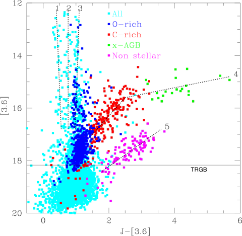
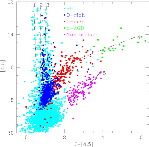
Figure 1: [3.6] vs. J–[3.6] (left) and [4.5] vs. J–[4.5] (right) CMDs. All cross matched points are shown as cyan dots. Blue dots are oxygen-rich (O-rich) stars, and red dots are carbon-rich (C-rich) stars. The green dots represent x-AGB stars. The magenta dots are mainly background galaxies (see text). The solid line in the left panel marks the tip of the red giant branch (TRGB) at $[3.6]=18.17$ mag (Boyer et al. 2009). Dashed numbered lines delineate sequences that we describe in the text.

Here we examine CMDs, in order to arrive at the currently best available sample of stars at their endpoints of evolution in the AGB phase, that we can use to derive the SFH. We follow a similar identification of features in the IR CMDs as in Blum et al. (2006), but using [4.5] instead of [8].

We cross matched the stars from Sibbons et al. (2015) with stars in the “good source catalogue” from Boyer et al. (2015a), using a matching radius of $1^{\prime\prime}$. We thus identified 5788 stars in common, of which 750 are AGB stars. About 30% of Sibbons et al.’s sources were not matched with any of Boyer et al.’s sources, which is largely a result of the different spatial coverage.

The [3.6] vs. J–[3.6] and [4.5] vs. J–[4.5] CMDs are presented in figure 1. Five sequences can be identified. The first of these, sequence 1 ($J-[3.6]<0.5$ mag, reaching $[3.6]\sim 12$ mag) corresponds to young A–G-type supergiants. Separated by a few tenths of magnitude to the red, sequence 2 consists mainly of foreground dwarfs and giants. Redder still by a similar amount, sequence 3 corresponds to RGB stars, AGB stars and late-type (mostly M) supergiants in IC 1613 (Menzies et al. 2015; Britavskiy et al. 2014; Herrero et al. 2010; Humphreys 1980).

Sibbons et al. (2015) divided the region above the tip of the RGB into O-rich and C-rich where the latter have $(J-K)>1.15$ mag. In figure 1 the blue and red points correspond to Sibbons’ photometric division of O-rich and C-rich, respectively, where the division occurs around $(J-[3.6])\sim 1.4$ mag (similar for J–[4.5]). Of the 741 AGB stars from Sibbons et al. that have $J$, $H$, $K$, [3.6] and [4.5], we classed 477 ($\sim 64\%$) as O-rich and 264 ($\sim 36\%$) as C-rich. This is very similar to Dell’Agli et al. (2016) where they compared models to the combination of near-IR (Sibbons et al. 2015) and mid-IR (Boyer et al. 2015a) data and found that the AGB sample of IC 1613 is composed of 65% O–rich and 35% C-rich stars.

The C-stars (red) and x-AGB stars (green) form sequence 4. Up to $(J-[3.6])\sim 3.1$ mag ($(J-[4.5])\sim 3.5$ mag) the sequence is dominated by stars that were classified from near-IR photometry as C-rich; beyond that is the realm of x-AGB stars. We stress that, while this sequence in other galaxies is normally dominated by carbon stars (Zijlstra et al. 2016; Wood et al. 2011) this does not preclude the presence of extremely dusty O-rich AGB stars among these red sources (van Loon et al. 1997). We classified all stars with $(J-[4.5])>3.5$ mag and $[4.5]<15.5$ mag as x-AGB; these 21 objects are listed in table 2. Of these x-AGB stars, all were found by Boyer et al. (2015b) to be variable (and x-AGB) at mid-IR wavelengths except #7773 and #7091 (from the Sibbons et al. (2015) catalogue), though Menzies et al. (2015) did identify #7773 as a LAV.

Table 2: Properties of the x-AGB stars identified in IC 1613.

RA	Dec	Boyer	[3.6]	[4.5]	Sibbons	$J$	$H$	$K$
(deg)	(deg)	#	(mag)	(mag)	#	(mag)	(mag)	(mag)
16.1832	2.0969	142022	$14.93\pm 0.03$	$14.32\pm 0.03$	11555	$18.067\pm 0.026$	$16.786\pm 0.015$	$15.557\pm 0.009$
16.2993	2.1124	53171	$15.35\pm 0.02$	$14.97\pm 0.03$	12772	$19.536\pm 0.099$	$18.105\pm 0.052$	$16.936\pm 0.030$
16.2354	2.2274	99513	$15.53\pm 0.03$	$14.87\pm 0.03$	19795	$19.183\pm 0.064$	$17.871\pm 0.038$	$16.535\pm 0.020$
16.1821	2.0567	142830	$14.93\pm 0.02$	$14.39\pm 0.03$	9057	$20.610\pm 0.234$	$18.594\pm 0.077$	$16.917\pm 0.029$
16.1820	2.0887	142987	$15.29\pm 0.03$	$14.98\pm 0.03$	10922	$19.359\pm 0.080$	$17.917\pm 0.042$	$16.764\pm 0.026$
16.0916	2.0912	208444	$15.43\pm 0.03$	$14.80\pm 0.03$	11103	$18.900\pm 0.054$	$17.456\pm 0.028$	$16.312\pm 0.017$
16.2946	2.0223	56137	$14.51\pm 0.03$	$14.13\pm 0.03$	7773	$18.896\pm 0.058$	$17.475\pm 0.030$	$16.132\pm 0.015$
16.2409	2.1547	95038	$15.50\pm 0.03$	$14.92\pm 0.03$	15999	$19.935\pm 0.121$	$18.438\pm 0.062$	$17.097\pm 0.032$
16.0911	2.2047	208785	$15.08\pm 0.02$	$14.72\pm 0.03$	18795	$18.262\pm 0.034$	$17.030\pm 0.021$	$16.025\pm 0.015$
16.2147	2.0639	115947	$15.36\pm 0.03$	$14.70\pm 0.03$	9409	$19.794\pm 0.118$	$18.177\pm 0.053$	$16.666\pm 0.024$
16.1727	2.1928	150523	$15.74\pm 0.03$	$15.39\pm 0.03$	18237	$19.354\pm 0.086$	$18.114\pm 0.053$	$17.033\pm 0.035$
16.3041	2.0853	50487	$15.27\pm 0.03$	$14.62\pm 0.03$	10697	$19.505\pm 0.096$	$18.224\pm 0.058$	$16.556\pm 0.022$
16.2899	2.2320	59151	$14.53\pm 0.03$	$13.61\pm 0.03$	19976	$18.563\pm 0.037$	$17.085\pm 0.019$	$15.611\pm 0.009$
16.2061	2.2790	122963	$15.62\pm 0.02$	$15.16\pm 0.03$	21513	$19.129\pm 0.071$	$17.936\pm 0.046$	$16.785\pm 0.028$
16.1948	2.0021	132310	$14.77\pm 0.02$	$14.14\pm 0.03$	7091	$20.165\pm 0.163$	$18.349\pm 0.062$	$16.829\pm 0.027$
16.1777	2.1171	146410	$15.43\pm 0.03$	$14.84\pm 0.03$	13166	$19.356\pm 0.081$	$17.872\pm 0.041$	$16.513\pm 0.021$
16.2195	2.1156	112075	$14.85\pm 0.03$	$14.34\pm 0.03$	13031	$18.889\pm 0.054$	$17.537\pm 0.030$	$16.111\pm 0.015$
16.2480	2.2076	89380	$15.37\pm 0.02$	$15.01\pm 0.03$	18925	$19.100\pm 0.059$	$17.461\pm 0.026$	$16.545\pm 0.020$
16.2351	2.2527	99713	$15.74\pm 0.02$	$14.47\pm 0.03$	20671	$20.309\pm 0.169$	$19.625\pm 0.178$	$18.210\pm 0.088$
16.1770	2.1128	146972	$15.15\pm 0.03$	$14.85\pm 0.03$	12808	$19.508\pm 0.092$	$18.031\pm 0.047$	$16.615\pm 0.023$
16.1880	2.1350	138007	$15.67\pm 0.03$	$14.98\pm 0.03$	14597	$18.993\pm 0.064$	$17.724\pm 0.038$	$16.686\pm 0.026$

Finally, sequence 5 (magenta in Fig. 1) are predominantly background galaxies (Meixner et al. 2006).

The numbers, and their contributions, of various populations identified in the CMDs are summarised in table 3.

Table 3: Summary of CMD selections of stellar populations and colour plotted in Fig. 1 .

Population	Diagram	$N$	%	Colour
Sources with J & [3.6]	[3.6], J–[3.6]	5261	100	Cyan
AGB with J & [3.6]	[3.6], J–[3.6]	741	14
C-rich AGB	[3.6], J–[3.6]	264	5	Red
O-rich AGB	[3.6], J–[3.6]	477	8	Blue
x-AGB	[4.5], J–[4.5]	21	0.4	Green
Background galaxies	[4.5], J–[4.5]	115	2	Magenta

2.4 Sample selection to determine the SFH

Previous application of our method (Javadi et al. 2011, 2017; Rezaei Kh et al. 2014; Golshan et al. 2017) – described in Section 3 – was based on confirmed LPVs. LPVs are red giant or supergiant pulsating stars with periods ranging from months to a few years (e.g., Soszyński et al. 2009). In the case at hand, though, the limited cadency of the DUSTiNGS survey and the limited depth of the Menzies et al. (2015) survey will have led to LPVs being missed. Therefore, we combine confirmed LPVs with those AGB and RSG candidate stars that are also expected to be LPVs. These candidates are:

1. x-AGB stars (a combination of our selection and Boyer et al. 2015b) and LAVs without determined period that are expected to be LPVs near the end of the AGB phase (e.g., Schröder et al. 1999; Fraser et al. 2008; Soszyński et al. 2009).

2. RSGs that do not have a determined period but must be good candidates for being LPVs. We note that any meaningful period determination of RSGs may require decades of observations (e.g., Kiss et al. 2006; Pierce et al. 2000).

Based on their location in the CMDs and with respect to isochrones (Fig. 2; Padova models from Marigo et al. 2017), our sample occupies the same region as the LPVs in our previous works.

The sample is summarised in table 4; of the x-AGB stars, eight were identified as LPVs or LAVs, hence the number of unique sources is 53 (two of the RSGs are also LPVs but they have not been counted in that category in the table).

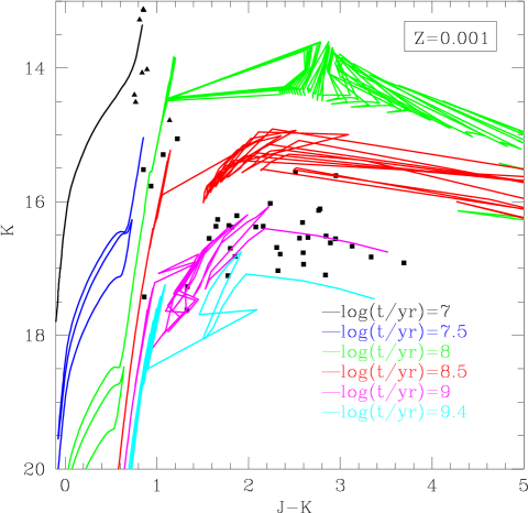
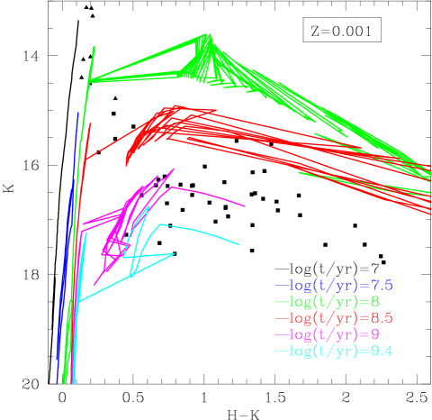
Figure 2: K vs. J–K (left) and H–K (right) with our selection of evolved stars (squares: AGB LPVs; triangles: RSGs), overlain with isochrones from Padova models (Marigo et al. 2017) labeled with logarithmic ages.

Table 4: Description of our sample to derive the SFH in IC 1613 (Total excludes duplicates).

Population	$N$	Reference
LPV	14	Menzies et al. (2015)
LAV	9	Menzies et al. (2015)
x-AGB	30	Boyer et al. (2015b) (cf. section 2.3)
RSG	8	Menzies et al. (2015)
Total	53

We limit the field of study to the smaller of the two, Boyer et al. (2015a) and Menzies et al. (2015), measuring 11.8 kpc² (after deprojection). Our sample is shown in figure 3, in relation to the general stellar distribution and the neutral hydrogen gas. As the half-light radius suggests, as many sources could be expected to be found (just) outside that radius as within that radius. While there is no direct confirmation of membership for any of these sources, their concentration on the (small portion of) sky strongly suggests that most – if not all – are associated with IC 1613.

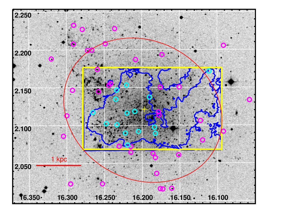
Figure 3: Spatial distribution of our stellar sample (magenta and cyan circles) and neutral hydrogen shells (H i; the largest blue contours in the yellow box). The stars of the sample which are inside the approximate boundary of the main H i supershell (Silich et al. 2006) are shown with cyan circles. The yellow cross indicates the optical centre of IC 1613, with the red ellipse outlining the half-light radius ($r_{\rm h}=6.5^{\prime}$, position angle $PA=58^{\circ}$). The (archival) optical image (at 468 nm wavelength) in the background was made with the UK Schmidt Telescope.

3 Method: deriving the SFH

The method we employ here was developed in Javadi et al. (2011, 2017). We limit ourselves to a brief description along with the model parametrisations determined for our case.

The SFH is the rate at which gas is converted into stars, $\xi$ (in M_⊙ yr^-1), as a function of time. The amount of stellar mass, $dM$, produced in a time interval $dt$ is:

$$dM(t)=\xi(t)\ dt.$$ (1)

We can find the number of formed stars from the total produced stellar mass by:

$$dN(t)=\frac{\int_{\rm min}^{\rm max}f_{\rm IMF}(m)\ dm}{\int_{\rm min}^{\rm max}f_{\rm IMF}(m)m\ dm}\ dM(t),$$ (2)

where $f_{\rm IMF}$ is the initial mass function (IMF). We use the IMF defined in Kroupa (2001):

$$f_{\rm IMF}=Am^{-\alpha},$$ (3)

where $A$ is the normalisation coefficient and $\alpha$ is a factor which depends on the mass range:

$$\alpha=\left\{\begin{array}[]{cclcl}+0.3\pm 0.7&{\rm for}&{\rm min}&<\frac{m}{{\rm M}_{\odot}}<&0.08\\ +1.3\pm 0.5&{\rm for}&0.08&<\frac{m}{{\rm M}_{\odot}}<&0.5\\ +2.3\pm 0.3&{\rm for}&0.5&<\frac{m}{{\rm M}_{\odot}}<&{\rm max}\\ \end{array}\right.$$ (4)

The minimum and maximum mass in Kroupa’s IMF were assumed to be 0.02 and 200 M_⊙, respectively.

Given that we use LPVs as proxies for the underlying stellar populations, we need to relate the number of variable stars to the total number of stars, $N$, which were formed in $dt$. We note that in this section ‘LPVs’ stand for all identified LPVs and other candidates that we expect to be in this phase (cf. section 2.4). If stars with mass between $m(t)$ and $m(t+dt)$ ($t$ is look-back time) are now LPVs, then the number of LPVs created between times $t$ and $t+dt$ is:

$$dn(t)=\frac{\int_{m(t)}^{m(t+dt)}f_{\rm IMF}(m)\ dm}{\int_{\rm min}^{\rm max}f_{\rm IMF}(m)\ dm}\ dN(t).$$ (5)

By substituting equations 1 and 2 into equation 5 we have:

$$dn(t)=\frac{\int_{m(t)}^{m(t+dt)}f_{\rm IMF}(m)\ dm}{\int_{\rm min}^{\rm max}f_{\rm IMF}(m)m\ dm}\ \xi(t)\ dt.$$ (6)

The number of LPVs, $dn^{\prime}$, we can observe in an age bin, $dt$, depends on the size of the bin ($dt$) and on the duration of the LPV stage ($\delta t$):

$$dn^{\prime}(t)=\frac{\delta t}{dt}\ dn(t).$$ (7)

Finally, by combining the above equations, we obtain a relation to give the SFR based on LPV counts:

$$\xi(t)=\frac{\int_{\rm min}^{\rm max}f_{\rm IMF}(m)m\ dm}{\int_{m(t)}^{m(t+dt)}f_{\rm IMF}(m)\ dm}\ \frac{dn^{\prime}(t)}{\delta t}.$$ (8)

In order to relate a LPV’s brightness to its mass, and its mass to its age (look-back time $t$) we appeal to stellar evolution models. The most suitable models are those from the Padova group, as argued extensively in Javadi et al. (2011, 2017); Rezaei Kh et al. (2014); Golshan et al. (2017). Here we use the latest version (PARSEC v1.2S + COLIBRI PR16; Marigo et al. 2017), which was improved upon the previous one (Marigo et al. 2008) resulting in a better estimation of the birth mass and pulsation timescale. Some cases of improvements that matter for us here are: new TP-AGB evolutionary tracks and atmosphere models for O-rich and C-rich stars; the complete thermal pulse cycles, with a full description of the in-cycle changes in the stellar parameters; new pulsation models to describe the fundamental and first overtone modes of LPVs; new dust models that consider the growth of the grains during the AGB evolution. That said, the evolutionary tracks of the youngest (most massive) stars ($\log M/{\rm M}_{\odot}\ga 0.7$) were not updated and still hail from the 2008 publication.

The LPVs are assumed to have reached their maximum near-IR brightness. Hence we apply a mass–K-band magnitude relation appropriate for the metallicity and distance modulus of IC 1613 ($Z=0.001$ and $\mu=24.37$ mag; left panel of figure 4; all the figures and tables for other metallicities we use in this paper are presented in the Appendix). While the K-band magnitude varies during the radial pulsation cycle, the photometry we are using are the mean magnitudes over several epochs and thus representative of the luminosity associated with the nuclear burning inside the star. The evolution of super-AGB stars toward the brighter K-band magnitudes has been omitted from the models, thus we interpolate the models over that range in mass (see Javadi et al. 2011 for details). The coefficients of the linear fitting between K-band magnitude and mass are listed in table 5.

Table 5: Fitted equations for the relation between birth mass and K-band magnitude, $\log M/{\rm M}_{\odot}=aK+b$, for a distance modulus of $\mu=24.37$ mag.

$Z=0.001$
$a$	$b$	validity range
$-0.322\pm 0.009$	$5.560\pm 0.168$	$K\leq 13.20$
$-1.726\pm 0.051$	$24.19\pm 0.720$	$13.20<K\leq 13.61$
$-0.176\pm 0.005$	$3.092\pm 0.009$	$13.61<K\leq 14.13$
$-0.072\pm 0.002$	$1.617\pm 0.048$	$14.13<K\leq 14.74$
$-0.339\pm 0.016$	$5.552\pm 0.168$	$14.74<K\leq 15.28$
$-0.116\pm 0.004$	$2.140\pm 0.063$	$15.28<K\leq 16.07$
$-0.175\pm 0.006$	$3.090\pm 0.009$	$16.07<K\leq 16.79$
$-0.107\pm 0.003$	$1.944\pm 0.057$	$16.79<K\leq 17.40$
$-0.225\pm 0.006$	$4.008\pm 0.120$	$K>17.40$

The onset of dust formation reddens and dims the stars, and we therefore need to apply a correction to bring them back to their photospheric peak brightness level. Because the evolutiuonary timescale shortens dramatically once dust formation sets in, the same brightness level found in the model at the end point of stellar evolution corresponds to the nuclear burning luminosity that can be directly related to the birth mass. Because some of the stars in our sample do not have J-band detections, we use H–K colours to determine this correction. As clearly discernible in figure 2, the reddened parts of the tracks/isochrones are bimodal in terms of their slope, based on whether the dust is O-rich or C-rich (Menzies et al. 2015; Albert et al. 2000). Therefore, we apply the following correction:

$$K_{\rm cor}=K+a_{\rm oxygen}[(H-K)-(H-K)_{0}],$$ (9)

for O-rich stars. For C-rich stars according to the isochrones in the right panels of Fig. 2 we have:

$$K_{\rm cor}=K+a_{\rm carbon}[(H-K)-(H-K)_{0}],$$ (10)

where $a_{\rm oxygen}=-1.2$ and $a_{\rm carbon}=-0.85$ are the average slopes of the isochrone after the peak in the K vs. H–K CMDs, and the average colours at the peak brightness are $(H-K)_{0}=1.05$ mag for O-rich stars and $(H-K)_{0}=0.8$ mag for C-rich stars. In some cases there is spectroscopic evidence for the chemical class of the object (Menzies et al. 2015; Albert et al. 2000); where this is not the case we have relied on photometric classification criteria (Sibbons et al. 2015; Menzies et al. 2015; Boyer et al. 2015b). The same selection criteria are also used for classification of x-AGB stars.

The relation between mass and age for LPVs is presented in the middle panel of figure 4, with the coefficients of linear fits listed in table 6, for a metallicity of $Z=0.001$.

Table 6: Fits to the relation between age and birth mass, $\log t=a\log M/{\rm M}_{\odot}+b$.

$Z=0.001$
$a$	$b$	validity range
$-3.289\pm 0.099$	$9.801\pm 0.294$	$\log{M/{\rm M}_{\odot}}\leq 0.10$
$-2.649\pm 0.078$	$9.743\pm 0.291$	$0.10<\log{M/{\rm M}_{\odot}}\leq 0.31$
$-2.510\pm 0.075$	$9.698\pm 0.291$	$0.31<\log{M/{\rm M}_{\odot}}\leq 0.55$
$-2.132\pm 0.063$	$9.487\pm 0.258$	$0.55<\log{M/{\rm M}_{\odot}}\leq 0.81$
$-1.701\pm 0.051$	$9.137\pm 0.273$	$0.81<\log{M/{\rm M}_{\odot}}\leq 1.11$
$-1.153\pm 0.036$	$8.528\pm 0.255$	$1.11<\log{M/{\rm M}_{\odot}}\leq 1.45$
$-0.678\pm 0.020$	$7.836\pm 0.234$	$\log{M/{\rm M}_{\odot}}>1.45$

We derived the relative pulsation duration (ratio of pulsation timescale to age) for a given birth mass from the Padova models; these relations are presented in the right panel of figure 4, and parameterised by a set of four Gaussian functions listed in table 7, for a metallicity of $Z=0.001$ (relations for other metallicities used in this paper can be found in the Appendix).

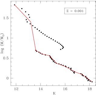
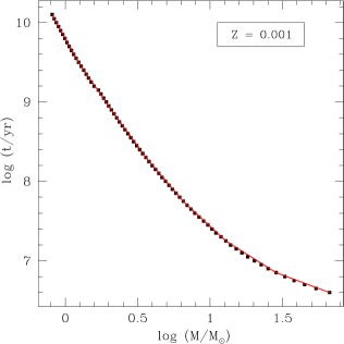
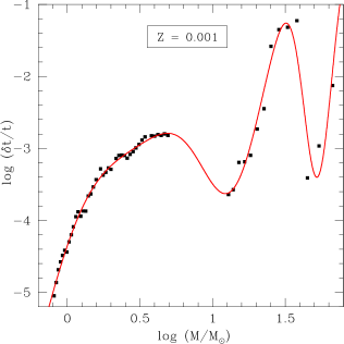
Figure 4: (Left:) relation between birth mass and K-band magnitude at the end point of stellar evolution for $Z=0.001$ and a distance modulus of $\mu=24.37$ mag. Solid lines are fits, in which the function is interpolated over the super-AGB phase ($0.7\la log{M/{\rm M}_{\odot}}\la 1.3$). (Middle:) same as the left, for the relation between age (at the end point of stellar evolution) and birth mass. (Right:) same as the left, for the relation between relative pulsation duration and birth mass. The points show the ratio of pulsation duration to age, versus mass; the solid lines are multiple-Gaussian fits, also interpolated over the super-AGB regime.

Table 7: Fits to the relation between relative pulsation duration ($\delta t/t$ where $t$ is the age and $\delta t$ is the pulsation duration) and birth mass, $\log(\delta t/t)=\Sigma_{i=1}^{4}a_{i}\exp\left[-(\log M/{\rm M}_{\odot}-b_{i})^{2}/c_{i}^{2}\right]$.

$Z=0.001$
$i$	$a$	$b$	$c$
1	$-53.46$	$-0.115$	0.749
2	$-02.62$	$+1.152$	0.316
3	$+48.48$	$-0.078$	0.697
4	$-03.23$	$+1.722$	0.139

To calculate the SFH, we thus employ the following procedure:

• Correct the K-band magnitude for dust attenuation;

• Use the corrected K-band magnitude and the mass–K-band equation (table 5) to obtain the birth mass;

• Use the birth mass and the age–mass equation (table 6) to obtain the age;

• Use the birth mass and the pulsation duration–mass equation (table 7) to obtain the pulsation timescale;

• Choose appropriate age bins and apply equation 8 to calculate the SFR in each of those bins.

For each bin, a statistical error can be derived from Poisson statistics as follows:

$$\sigma_{\xi(t)}=\frac{\sqrt{N}}{N}\xi(t),$$ (11)

where $N$ is the number of stars in each age bin.

4 Results

Using our sample of evolved stars (section 2.4) and applying our method (section 3), we estimate SFRs in IC 1613 over the broad time interval from 30 Myr to $\sim 5$ Gyr ago. The observational reasons for being unable to determine SFRs at earlier epochs will be described below. Because the metallicity is expected to increase over time as a result of the chemical evolution driven by nucleosynthesis and mass loss, we first apply our method assuming different metallicities and then re-analyse it adopting instead the linear age–metallicity relation (AMR) from Skillman et al. (2014) for values $4\times 10^{-4}<Z<4\times 10^{-3}$ (corresponding to 13 Gyr ago $<t<$ now).

Figure 5: (Left:) recent SFH (last Gyr) in a $\sim 200$ square arcmin ($\sim 11.8$ kpc²) of IC 1613 assuming a constant metallicity of $Z=0.003$. (Right:) same, but in $\sim 36$ square arcmin ($\sim 2.2$ kpc²) in the central part of the galaxy.

We start by examining the recent SFH, at a constant metallicity. The SFR as a function of look-back time in the last Gyr is shown in the left panel of figure 5. For this epoch we assumed $Z=0.003$. The horizontal bars represent the spread in age within each bin, while the vertical bars represent the statistical errors. The mean SFR over the last 200 Myr ($\log t({\rm yr})\sim 8.3$) in the central 11.8 kpc² is $\xi\sim(0.5\pm 0.2)\times 10^{-3}$ M_⊙ yr^-1 kpc^-2; it is marginally higher in the central 2.2 kpc², $\xi\sim(0.65\pm 0.3)\times 10^{-3}$ M_⊙ yr^-1 kpc^-2. This agrees well with the result derived by Bernard et al. (2007): they found a mean SFR of $\xi\sim(1.6\pm 0.8)\times 10^{-3}$ M_⊙ yr^-1 kpc^-2 in the central part ($r\leq 2\hbox to0.0pt{.\hss}^{\prime}5$) of the galaxy for the last 300 Myr ($\log t({\rm yr})\sim 8.5$), replicating the result obtained by Cole et al. (1999) for a central $\sim 0.22$ kpc² region on the basis of the main-sequence luminosity distribution. Cole et al. also found that the SFR was $\sim 50$% higher 400–900 Myr ago ($8.6<\log t({\rm yr})<8.9$). While based on just 19 stars in the central 2.2 kpc², we find $\xi\sim(0.9\pm 0.3)\times 10^{-3}$ M_⊙ yr^-1 kpc^-2 500–900 Myr ago (Fig. 5, right), i.e.  a very similar SFH as that determined by Cole et al.

Subsequently, we applied this process for all epochs and five metallicities ($Z=0.0004$, 0.0007, 0.001, 0.002, 0.003); the result is shown in figure 6. Clearly, the result is sensitive to the adopted metallicity, so in order to trace back the SFH we need to take into account the variation of metallicity with look-back time.

Skillman et al. (2014) modelled the CMDs in a small field near the half-light radius to determine the SFH for the full 13 Gyr of evolution. They found that most – if not all – stars in IC 1613 formed after the epoch of reionization ($\sim 12.8$ Gyr ago), without a dominant formation epoch. To compare with their result, we adopt a similar AMR as they did: $Z=0.003$ for the last Gyr ($\log t({\rm yr})<9$), $Z=0.002$ for 1 Gyr $<t<2$ Gyr ($9<\log t({\rm yr})<9.3$) and $Z=0.0007$ for $t>2$ Gyr ($\log t({\rm yr})>9.3$). We thus find a mean value of the SFR across IC 1613 over the last Gyr of $\xi=(3.0\pm 0.5)\times 10^{-4}$ M_⊙ yr^-1 kpc^-2 (Fig. 7), in excellent agreement with Skillman et al., who found $\xi\sim 3.4\times 10^{-4}$ M_⊙ yr^-1 kpc^-2.

Figure 6: IC 1613 SFHs for different metallicities.

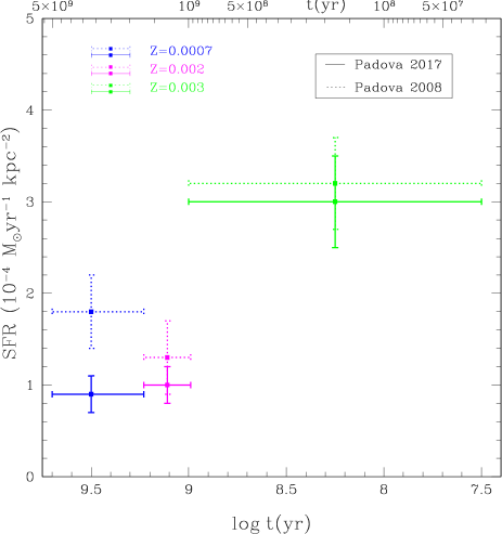
Figure 7: The SFH in IC 1613 with the adoption of an AMR akin that derived by Skillman et al. (2014), using the pulsation durations from Marigo et al. (2017) (solid) and Marigo et al. (2008) (dotted).

However, Skillman et al. (2014) found SFRs at earlier epochs (1 Gyr $<t<2$ Gyr and 2 Gyr $<t<5$ Gyr) that are two to three times higher than our results, and we could not trace star formation beyond $\sim 5$ Gyr ago. We now discuss how the SFH we derive for look-back times $t>9$ Gyr may have been biased.

The truncated SFH (beyond 5 Gyr) is mainly due to observational limitations with regard to our method:

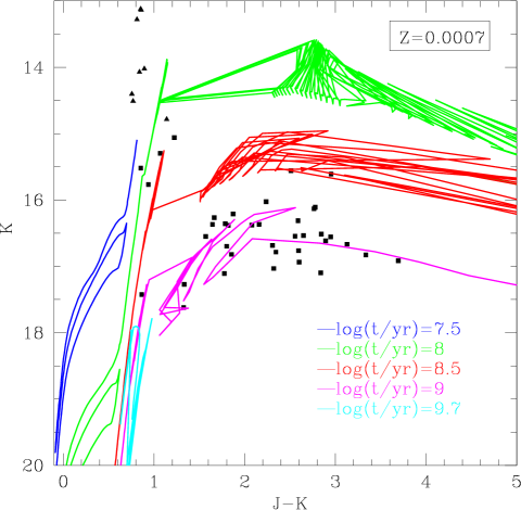
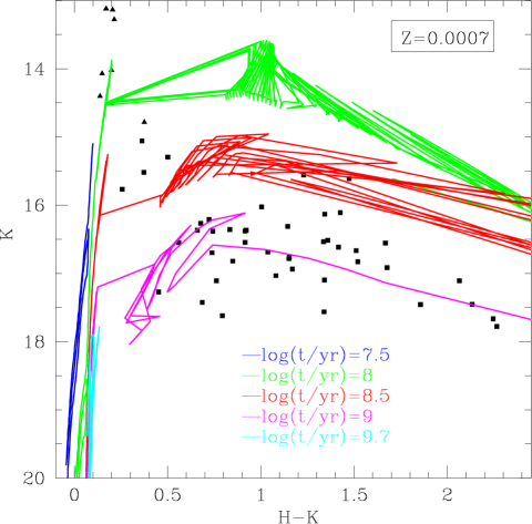
Figure 11: Same as figure 2 but for $Z=0.0007$.

• The sample of LPVs comes from the survey by Menzies et al. (2015), which quote a completeness limit of $K_{\rm s}\approx 18$ mag and will have missed red variables with $(H-K_{\rm s})>2.0$ mag and $K_{\rm s}>16.3$ mag. In order to trace the SFH to $t>5$ Gyr ($\log t({\rm yr})>9.7$) at low metallicity ($Z\sim 0.0007$), however, we need stars that have dereddened K-band magnitudes fainter than $\sim 18$ mag (see the isochrone diagram in figure 11).

• Regarding x-AGB stars, the Spitzer sample from Boyer et al. (2015a) is not flux limited, and the near-IR data from Sibbons et al. (2015) are deep enough ($J<19.7$, $H<19.3$ and $K<18.9$ mag) to provide counterparts to place them in the CMD. However, most x-AGB stars are carbon stars, with the odd more massive OH/IR star – cf. Woods et al. (2011), and carbon stars arise from stars born not longer than $\sim 5.5$ Gyr ago (Dell Agli et al. 2016). Thus, these x-AGB samples do not make up for the incompleteness of the variability survey by Menzies et al. beyond 5 Gyr.

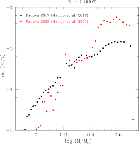
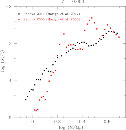
Figure 8: The differences between the pulsation durations ($\delta t$) from the most recent Padova models (Marigo et al. 2017, black) and previous version (Marigo et al. 2008, red) $Z=0.0007$ (left) and $Z=0.003$ (right).

The reasons for the discrepancy between our SFR determinations a few Gyr ago and those by Skillman et al. (2014) are more subtle, and probably include the following:

• It is likely that the completeness limits of the monitoring survey and possibly the near-IR complement to the Spitzer survey start to deplete our sample of sources at multi-Gyr ages. This is not an issue for the most recent Gyr, which is confirmed by the good correspondence with the results in the literature as described above.

• While the field studied by Skillman et al. (2014) may be representative of the bulk of IC 1613 in recent times, this may not be true at earlier epochs. We tried to find the SFR on the same location as their field ($RA\sim 1^{\rm h}4^{\rm m}30^{\rm s}$ and $Dec\sim 2^{\circ}9^{\prime}$), but the sample became limited to just one star and this did not yield a meaningful SFR.

• The pulsation durations ($\delta t$) may have been overestimated, which would immediately result in an underestimated SFR. Figure 8 shows the differences between the Marigo et al. (2017) and Marigo et al. (2008) pulsation durations. For stars with $0.3\la\log M/{\rm M}_{\odot}\la 0.7$ the pulsation duration was shortened, while for intermediate- and low-mass stars with $\log M/{\rm M}_{\odot}\la 0.3$ the duration was lengthened. Our results are in better agreement with the results from Skillman et al. (2014) when using the 2008 models (dotted lines in figure 7). For $t>2$ Gyr ($\log t({\rm yr})>9.3$) the SFR using the Marigo et al. (2008) pulsation durations doubles and becomes$\sim 60$% of the SFR derived by Skillman et al. ($\xi\sim 3\times 10^{-4}$ M_⊙ yr^-1 kpc^-2); for 1 Gyr $<t<2$ Gyr ($9<\log t({\rm yr})<9.3$) the SFR would also increase but only to $\sim 30$% of the SFR derived by Skillman et al. ($\xi\sim 3.6\times 10^{-4}$ M_⊙ yr^-1 kpc^-2). This is not the first time that results suggest that the pulsation durations in the Padova models may be too generous: Javadi et al. (2017) (see also Javadi et al. 2013) found corrections of a factor $\sim 3$ were needed at solar and slightly sub-solar metallicity. It appears that the 2008 Padova models are preferred over the 2017 models, at least for older ages at low metallicities, but still need to be corrected by a factor $\sim 2$–3.

In any case we do not find a discrete epoch of enhanced (or suppressed) star formation (Fig. 7), that could be linked to external triggering mechanisms. This supports the notion that IC 1613 has evolved in isolation for at least the past 5 Gyr (Skillman et al. 2014; Cole et al. 1999; Stinson et al. 2007).

5 Discussion

5.1 Galactocentric radial gradient of the SFH

Galactocentric radial gradients are imprinted with the dynamical history and propagation of star formation. It appears that stellar population gradients are universal in dwarf galaxies, in the sense that the mean age of the stellar population is younger towards the centre of the galaxy (e.g., Skillman et al. 2014; Hidalgo et al. 2013).

To examine radial gradients in IC 1613, we divided our sample into two parts – an inner ($r<1$ kpc) and an outer ($r>1$ kpc) region. The resulting SFHs are shown in figure 9. In the inner part, the mean SFR over the past Gyr ($Z\sim 0.003$) was $\xi\sim 0.7\times 10^{-4}$ M_⊙ yr^-1 kpc^-2, in the outer part it was $\xi\sim 0.2\times 10^{-4}$ M_⊙ yr^-1 kpc^-2. Clearly, the inner part contains more young stars relative to the outer region, but this is in part due to the radially decreasing overall stellar density. However, when considering the SFRs at older times and lower metallicity, they increase more rapidly in the outer parts than in the inner parts of IC 1613. In fact, at the lower metallicities ($Z\sim 0.0007$) the SFR in the outer galaxy rivals that near the centre.

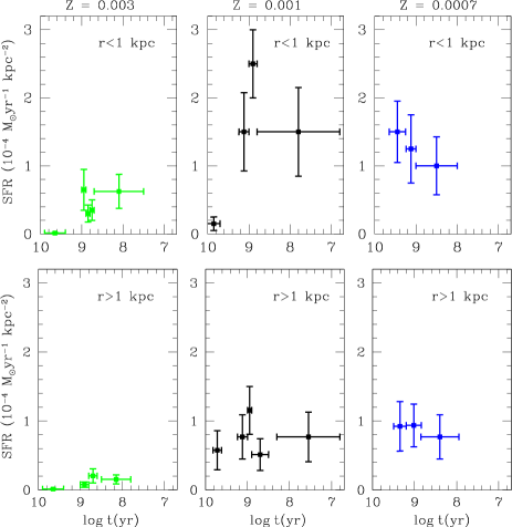
Figure 9: SFHs of two regions at different galactocentric radii ($r<1$ kpc, $r>1$ kpc), for different metallicities.

Another way of quantifying this gradient is in terms of the ratio of SFRs at older times ($\log t({\rm yr})>9.2$, $Z=0.0007$) to those at recent times ($\log t({\rm yr})<9$, $Z=0.003$). In the inner region this ratio is $\sim 2$, while in the outer region it is $\sim 7$. Considering the errorbars (minimum of old SFR and maximum of recent SFR) decreases the ratio to $\sim 1$ for the inner part and $\sim 3$ for the outer part. This outside–in evolution scenario (at least for the most recent $\sim 5$ Gyr) is in agreement with what is typically found in dwarf galaxies (e.g., Hidalgo et al. 2003, 2008, 2013) and differs from what is found in the low-mass spiral galaxy M 33, for instance (Javadi et al. 2017).

As we described in the result section, because of incompleteness of the surveys it is possible that we have underestimated the SFR older than a Gyr. Likewise, the discrepant pulsation durations between the 2008 and 2017 Padova models could have affected the older SFRs. But this is true for both the inner and outer part in this section, and we do not expect the observed gradient to change. Furthermore, the SFH over the last Gyr in the central part (right panel of Fig. 5) compared to that in our larger field of view (left panel of Fig. 5) shows an obvious concentration of recent star formation in the central part of the galaxy.

5.2 The origin of the main hydrogen supershell

The neutral interstellar medium within dwarf galaxies often shows holes, arcs, and shells. These structures are typically explained by the (combined) effects of stellar winds from massive stars and supernova (SN) explosions (Dyson & de Vries 1972; Weaver et al. 1977), but this scenario struggles to explain the largest structures (Silich et al. 2006 and references therein).

With regard to IC 1613, Silich et al. (2006) identified several H i supershells, including “main supershell” – an H i hole of 1 kpc in diameter and surrounded by an H i ring centred at $RA=1^{\rm h}4^{\rm m}52^{\rm s}$ ($16\hbox to0.0pt{.\hss}^{\circ}2167$), $Dec=2^{\circ}7^{\prime}$ ($2\hbox to0.0pt{.\hss}^{\circ}1167$) (see Fig. 3). The H i mass of this supershell is $2.8\times 10^{7}$ M_⊙. The absence of regular expansion and the thickness of the ring led Silich et al. to believe the shell has stalled. The wide range in age of the OB associations – up to 30 Myr (Borissova et al. 2004) – found inside the shell, suggested to them that the shell was formed over a period of $\sim 30$ Myr.

Silich et al. simulated the formation of the main supershell for two different (thin and thick) galactic disc models, in both cases concluding a formation timescale of 30 Myr. They thus estimated a mid-plane gas number density $n_{0}\sim 2.8(1.4)$ cm^-3 and a SFR of $xi\sim 7.5(2.3)\times 10^{-3}$ M_⊙ yr^-1 for their thin (thick) disc models. This is an order of magnitude larger than the in-situ SFR they derived from H$\alpha$ data, $xi\sim(3$–$4)\times 10^{-4}$ M_⊙ yr^-1, leading them to reject the multiple-SN scenario.

To revisit the SFR within the main supershell, we selected stars – 15 in total – from our sample that reside inside the contour outlining the main supershell in Silich et al. (2006) (Fig. 3). Assuming a constant metallicity of $Z=0.003$, we thus derive the recent SFH within the shell (Fig. 10). Because of the small number statistics we lack supergiants within this limited sample and thus cannot ascertain the SFR at $t<100$ Myr. However, the SFR seems to have slowly but steadily decreased in recent times, and if this trend continued into the most recent 30 Myr we would estimate a SFR that is compatible with the one derived from H$\alpha$ by Silich et al. (2006). One may wonder, though whether the shell could in fact have formed over much longer timescales, in excess of 100 Myr – from which OB associations no longer exist.

Figure 10: SFHs within the main supershell (Silich et al. 2006) of IC 1613 assuming a constant metallicity of $Z=0.003$.

5.3 Ability of mass loss to sustain star formation

Star formation depletes a galaxy of its gas, but stellar mass loss replenishes it. The question therefore is whether the latter can sustain the former.

Silich et al. (2006) derived a total H i mass in IC 1613 of $6.0\times 10^{7}$ M_⊙, in good agreement with previous estimates from Lake & Skillman (1989). Considering also the contribution from helium, the total mass of the ISM would be $\sim 9.0\times 10^{7}$ M_⊙. Dell’Agli et al. (2016) used stellar evolution models to estimate the dust production rate by AGB stars within IC 1613, $\sim 6\times 10^{-7}$ M_⊙ yr^-1, and gas-to-dust mass ratio, $\sim 1000$, and hence a total mass return rate of $6\times 10^{-4}$ M_⊙ yr^-1.

The recent SFR of $\xi=(5.5\pm 2)\times 10^{-3}$ M_⊙ yr^-1 we derived from the evolved star population (Fig. 5) exceeds the mass return rate by an order of magnitude. This means that the ISM will be depleted by star formation on a timescale of 16.4 Gyr. Accounting for the mass return rate would stretch this by a small amount to $\sim 18.4$ Gyr. Considering the contribution of ionized mass of the galaxy (about a few times $10^{6}$ from Silich et al. 2006) can increase the estimation up to 10%.

This assumes that star formation is 100% efficient, and that no ISM gas is blown out of the shallow gravitational potential well of the dwarf galaxy, so star formation at the current rate would unlikely continue for that long. On the other hand, the above estimate also neglects contributions to mass return by SNe, luminous blue variables et cetera – though these do not make a huge difference when assessed over cosmological times (cf. Javadi et al. 2013). The expectation therefore is that IC 1613 cannot continue to form stars at the current rate for more than a few Gyr, unless gas is accreted from outside, for instance when (if) it traverses the halo from M 31 or the Milky Way, or intergalactic gas if such reservoirs exist.

6 Summary of conclusions

Selecting stars at the end points of their evolution, we applied a recently developed method to derive the SFH in the isolated Local Group dIrr galaxy IC 1613. Our main findings are:

• From a combination of near-/mid-IR CMDs we identified 21 x-AGB stars, of which 2 stars had not been identified before.

• We do not find any dominant period of star formation over the past 5 Gyr, which suggests that IC 1613 may have evolved in isolation for at least that long.

• The SFH over the past few Gyr confirms those derived by other methods, with a radial gradient that indicates the mean age of the central population is younger than that in the outskirts.

• The extrapolated rate of recent star formation within the main H i supershell falls short by an order of magnitude of the required recent SFR to have produced the shell.

• The current reservoir of interstellar gas may sustain star formation at the current rate for several Gyr into the future; however the rate at which mass is returned will not extend that time for very much longer – indeed, star formation beyond the next few Gyr will diminish and eventually cease altogether unless gas can be accreted from outside.

Appendix A Supplementary material

In this section we present figures and fits to the K-band–mass, age–mass and pulsation duration–mass relation, derived from the Padova models (Marigo et al. 2017; Marigo et al. 2008). We used these equations in our analysis to find the SFH of IC 1613. For more detail see section 3 where we explain the method and present the figures and fits for the case of $Z=0.001$ (and $\mu=24.37$ mag). Here we also present isochrones for $Z=0.0007$.

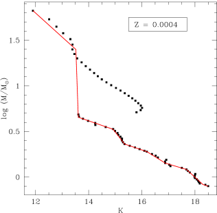
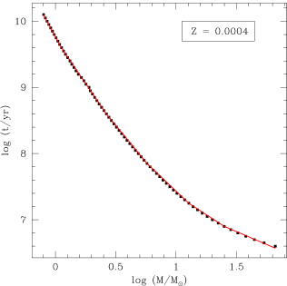
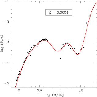
Figure 12: Same as figure 4 but for $Z=0.0004$.

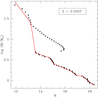
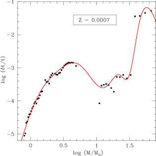
Figure 13: Same as figure 12 but for $Z=0.0007$.

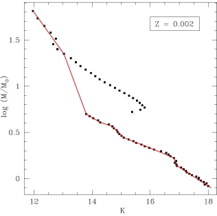
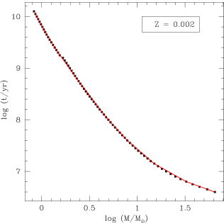
Figure 14: Same as figure 12 but for $Z=0.002$.

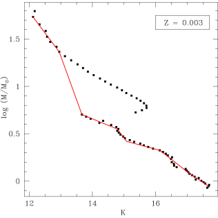
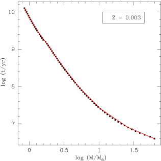
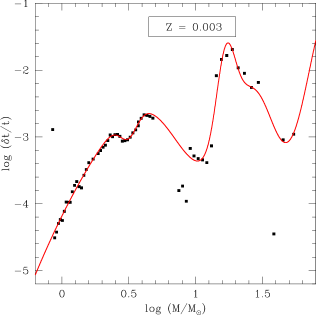
Figure 15: Same as figure 12 but for $Z=0.003$.

Table 8: Fits to the relation between birth mass and K-band magnitude, $\log M/{\rm M}_{\odot}=aK+b$, for a distance modulus of $\mu=24.37$ mag.

$a$	$b$	validity range
$Z=0.0004$
$-0.263\pm 0.008$	$4.960\pm 0.150$	$K\leq 13.52$
$-8.248\pm 0.246$	$112.9\pm 3.320$	$13.52<K\leq 13.61$
$-0.102\pm 0.003$	$2.038\pm 0.006$	$13.61<K\leq 14.92$
$-0.374\pm 0.011$	$6.100\pm 0.183$	$14.92<K\leq 15.35$
$-0.010\pm 0.003$	$1.894\pm 0.057$	$15.35<K\leq 16.19$
$-0.1816\pm 0.005$	$3.219\pm 0.096$	$16.19<K\leq 16.88$
$-0.087\pm 0.000$	$1.627\pm 0.048$	$16.88<K\leq 17.68$
$-0.269\pm 0.008$	$4.839\pm 0.144$	$17.68<K\leq 18.29$
$-0.100\pm 0.003$	$1.749\pm 0.051$	$K>18.29$
$Z=0.0007$
$-0.3875\pm 0.011$	$6.519\pm 0.195$	$K\leq 13.20$
$-1.882\pm 0.057$	$26.25\pm 0.078$	$13.20<K\leq 13.59$
$-0.105\pm 0.003$	$2.095\pm 0.063$	$13.59<K\leq 14.70$
$-0.393\pm 0.012$	$6.399\pm 0.189$	$14.70<K\leq 15.12$
$-0.116\pm 0.004$	$2.149\pm 0.063$	$15.12<K\leq 16.38$
$-0.214\pm 0.006$	$3.750\pm 0.114$	$16.38<K\leq 16.93$
$-0.040\pm 0.001$	$0.805\pm 0.002$	$16.93<K\leq 17.37$
$-0.231\pm 0.007$	$4.119\pm 0.123$	$K>17.37$
$Z=0.002$
$-0.437\pm 0.013$	$7.041\pm 0.210$	$K\leq 13.03$
$-0.847\pm 0.026$	$12.38\pm 0.360$	$13.03<K\leq 13.80$
$-0.187\pm 0.006$	$3.280\pm 0.099$	$13.80<K\leq 14.28$
$-0.103\pm 0.003$	$2.074\pm 0.063$	$14.28<K\leq 14.70$
$-0.313\pm 0.009$	$5.171\pm 0.156$	$14.70<K\leq 15.09$
$-0.124\pm 0.004$	$2.315\pm 0.069$	$15.09<K\leq 16.13$
$-0.132\pm 0.004$	$2.444\pm 0.072$	$16.13<K\leq 16.82$
$-0.826\pm 0.025$	$14.15\pm 0.420$	$16.82<K\leq 16.92$
$-0.203\pm 0.006$	$3.581\pm 0.108$	$K>16.92$
$Z=0.003$
$-0.445\pm 0.013$	$7.122\pm 0.213$	$K\leq 12.95$
$-0.920\pm 0.003$	$13.28\pm 0.390$	$12.95<K\leq 13.67$
$-0.136\pm 0.004$	$2.568\pm 0.078$	$13.67<K\leq 14.79$
$-0.448\pm 0.014$	$7.180\pm 0.216$	$14.79<K\leq 15.08$
$-0.0904\pm 0.003$	$1.783\pm 0.054$	$15.08<K\leq 16.13$
$-0.254\pm 0.008$	$4.429\pm 0.132$	$16.13<K\leq 16.49$
$-0.268\pm 0.008$	$4.646\pm 0.138$	$16.49<K\leq 16.95$
$-0.2265\pm 0.007$	$3.949\pm 0.117$	$K>16.95$

Table 9: Fits to the relation between age and birth mass, $\log t=a\log M/{\rm M}_{\odot}+b$.

$a$	$b$	validity range
$Z=0.0004$
$-3.333\pm 0.099$	$9.767\pm 0.294$	$\log{M/{\rm M}_{\odot}}\leq 0.050$
$-2.690\pm 0.081$	$9.734\pm 0.291$	$0.050<\log{M/{\rm M}_{\odot}}\leq 0.236$
$-2.680\pm 0.081$	$9.732\pm 0.291$	$0.236<\log{M/{\rm M}_{\odot}}\leq 0.422$
$-2.225\pm 0.066$	$9.540\pm 0.285$	$0.422<\log{M/{\rm M}_{\odot}}\leq 0.759$
$-1.732\pm 0.051$	$9.166\pm 0.280$	$0.759<\log{M/{\rm M}_{\odot}}\leq 1.106$
$-1.195\pm 0.036$	$8.571\pm 0.260$	$1.106<\log{M/{\rm M}_{\odot}}\leq 1.399$
$-0.778\pm 0.023$	$7.989\pm 0.240$	$\log{M/{\rm M}_{\odot}}>1.399$
$Z=0.0007$
$-3.409\pm 0.102$	$9.780\pm 0.294$	$\log{M/{\rm M}_{\odot}}\leq 0.010$
$-3.191\pm 0.096$	$9.781\pm 0.294$	$0.010<\log{M/{\rm M}_{\odot}}\leq 0.100$
$-2.787\pm 0.084$	$9.745\pm 0.291$	$0.100<\log{M/{\rm M}_{\odot}}\leq 0.196$
$-2.586\pm 0.078$	$9.706\pm 0.291$	$0.196<\log{M/{\rm M}_{\odot}}\leq 0.350$
$-2.376\pm 0.072$	$9.632\pm 0.288$	$0.350<\log{M/{\rm M}_{\odot}}\leq 0.660$
$-1.940\pm 0.057$	$9.342\pm 0.279$	$0.660<\log{M/{\rm M}_{\odot}}\leq 0.920$
$-1.558\pm 0.048$	$8.989\pm 0.270$	$0.920<\log{M/{\rm M}_{\odot}}\leq 1.181$
$-1.076\pm 0.033$	$8.419\pm 0.252$	$1.181<\log{M/{\rm M}_{\odot}}\leq 1.459$
$-0.679\pm 0.020$	$7.841\pm 0.234$	$\log{M/{\rm M}_{\odot}}>1.459$
$Z=0.002$
$-3.412\pm 0.136$	$9.827\pm 0.294$	$\log{M/{\rm M}_{\odot}}\leq 0.020$
$-3.041\pm 0.090$	$9.819\pm 0.294$	$0.020<\log{M/{\rm M}_{\odot}}\leq 0.150$
$-2.582\pm 0.078$	$9.748\pm 0.291$	$0.150<\log{M/{\rm M}_{\odot}}\leq 0.380$
$-2.431\pm 0.096$	$9.689\pm 0.291$	$0.380<\log{M/{\rm M}_{\odot}}\leq 0.670$
$-2.024\pm 0,060$	$9.415\pm 0.282$	$0.670<\log{M/{\rm M}_{\odot}}\leq 0.890$
$-1.598\pm 0.048$	$9.033\pm 0.270$	$0.890<\log{M/{\rm M}_{\odot}}\leq 1.170$
$-1.045\pm 0.030$	$8.381\pm 0.252$	$1.170<\log{M/{\rm M}_{\odot}}\leq 1.510$
$-0.667\pm 0.020$	$7.809\pm 0.234$	$\log{M/{\rm M}_{\odot}}>1.510$
$Z=0.003$
$-3.360\pm 0.102$	$9.865\pm 0.347$	$\log{M/{\rm M}_{\odot}}\leq 0.090$
$-2.523\pm 0.075$	$9.786\pm 0.030$	$0.090<\log{M/{\rm M}_{\odot}}\leq 0.250$
$-2.769\pm 0.084$	$9.848\pm 0.294$	$0.250<\log{M/{\rm M}_{\odot}}\leq 0.390$
$-2.450\pm 0.075$	$9.722\pm 0.291$	$0.390<\log{M/{\rm M}_{\odot}}\leq 0.700$
$-1.892\pm 0.060$	$9.329\pm 0.279$	$0.700<\log{M/{\rm M}_{\odot}}\leq 1.020$
$-1.256\pm 0.039$	$8.681\pm 0.261$	$1.020<\log{M/{\rm M}_{\odot}}\leq 1.410$
$-0.796\pm 0.024$	$8.028\pm 0.240$	$\log{M/{\rm M}_{\odot}}>1.410$

Table 10: Fits to the relation between the relative pulsation duration and birth mass, $\log(\delta t/t)=\Sigma_{i=1}^{5}a_{i}\exp\left[-(\log M[{\rm M}_{\odot}]-b_{i})^{2}/c_{i}^{2}\right]$.

$i$	$a$	$b$	$c$
$Z=0.0004$
1	$-$113.2	$-$2.296	2.073
2	$-$1.084	0.969	0.239
3	55.97	$-$1.295	1.580
4	$-$1.963	1.456	0.248
5	0.000	2.385	0.022
$Z=0.0007$
1	$-$560.9	147.7	74.38
2	$-$2.084	0.468	0.404
3	15.58	1.161	1.313
4	$-$1.373	1.479	0.141
5	$-$7.463	1.132	0.531
$Z=0.002$
1	$-$2.525	0.741	0.924
2	9.158	0.735	0.238
3	$-$2.027	1.719	0.304
4	$-$9.475	0.754	0.258
5	$-$5.478	$-$0.489	0.606
$Z=0.003$
1	$-$721.0	$-$10.65	4.693
2	$-$0.340	0.499	0.090
3	$-$1.961	1.089	0.359
4	1.288	1.225	0.099
5	$-$2.240	1.697	0.223

References

- [Albert et al.(2000)] Albert L., Demers S., Kunkel W. E. 2000, ApJ, 119, 2780
- [Antonello et al.(2000)] Antonello E., Fugazza D., Mantegazza L., Bossi M., Covino S. 2000, A&A, 363, 29
- [Bernard et al.(2007)] Bernard E. J., Aparicio A., Gallart C., Padilla-Torres C. P., Panniello M. 2007, AJ, 134, 1124
- [Blum et al.(2006)] Blum R. D., et al. 2006, AJ, 132, 2034
- [Blumenthal et al.(1984)] Blumenthal G. R., Faber S. M., Primack J. R., Rees M. J. 1984, Nature, 311, 517
- [Borissova et al.(2004)] Borissova J., Kurtev R., Georgiev L., Rosado M. 2004, A&A, 413, 889
- [Boyer et al.(2009)] Boyer M. L., Skillman E. D., van Loon J. Th., Gehrz R. D., Woodward C. E. 2009, ApJ, 697, 1993
- [Boyer et al.(2015a)] Boyer M. L., et al. 2015a, ApJS, 216, 10
- [Boyer et al.(2015b)] Boyer M. L., et al. 2015b, ApJ, 800, 17
- [Britavskiy et al.(2015)] Britavskiy N. E., Bonanos A. Z., Mehner A., García-Álvarez D, Prieto J. L., Morrell N. I. 2014, A&A, 562, A75
- [Carroll & Ostile (2007)] Carroll B. W., Ostlie D. A. 2007, An introduction to modern astrophysics. Pearson Addison-Wesley (San Francisco)
- [Chun et al.(2015)] Chun S.H., Jung M., Kang M., Kim J.W., Sohn Y.J. 2015, A&A, 578, A51
- [Cole et al.(1999)] Cole A. A., et al. 1999, AJ, 118, 1657
- [Dekel & Woo (2003)] Dekel A., Woo J. 2003, MNRAS, 344, 1131
- [Dell’Agli et al.(2016)] Dell’Agli F., Di Criscienzo M., Boyer M. L., García-Hernández D. A. 2016, MNRAS, 460, 4230
- [Dolphin et al.(2001)] Dolphin A. E., et al. 2001, ApJ, 550, 554
- [Dyson & de Vries(1972)] Dyson J. E., de Vries J. 1972, A&A, 20, 223
- [Fraser et al.(2005)] Fraser O. J., Hawley S. L., Cook K. H., Keller S. C. 2005, AJ, 129, 768
- [Fraser, Hawley & Cook (2008)] Fraser O. J., Hawley S. L., Cook K. H. 2008, AJ, 136, 1242
- [Goldman et al.(2017)] Goldman S. R., et al. 2017, MNRAS, 465, 403
- [Golshan et al.(2017)] Golshan R. H., Javadi A., van Loon J. Th., Khosroshahi H., Saremi E. 2017, MNRAS, 466, 1764
- [Groenewegen et al.(1998)] Groenewegen M. A. T., Whitelock P. A., Smith C. H., Kerschbaum F. 1998, MNRAS, 293, 18
- [Herrero et al.(2010)] Herrero A., Garcia M., Uytterhoeven K., Najarro F., Lennon D. J., Vink J. S., Castro N. 2010, A&A, 513, A70
- [Hidalgo et al.(2003)] Hidalgo S. L., Marín-Franch A., Aparicio A. 2003, AJ, 125, 1247
- [Hidalgo et al.(2008)] Hidalgo S. L., Aparicio A. & Gallart, C. 2008, AJ, 136, 2332
- [Hidalgo et al.(2013)] Hidalgo S. L., et al. 2013, ApJ, 778, 103
- [Hodge (1980)] Hodge P. 1989, ARA&A, 27, 139
- [Humphreys (1980)] Humphreys R. M. 1980, ApJ, 238, 65
- [Iben & Renzini(1983)] Iben Jr. I., Renzini A. 1983, ARA&A, 21, 271
- [Javadi, van Loon & Mirtorabi (2011)] Javadi A., van Loon J. Th., Mirtorabi M. T. 2011, MNRAS, 414, 3394
- [Javadi et al.(2013)] Javadi A., van Loon J. Th., Khosroshahi H., Mirtorabi M. T. 2013, MNRAS, 432, 2824
- [Javadi et al.(2017)] Javadi A., van Loon J. Th., Khosroshahi H., Tabatabaei F., Golshan R. H., Rashidi M. 2017, MNRAS, 464, 2103
- [Kirby et al.(2014)] Kirby E. N., Bullock J. S., Boylan-Kolchin M., Kaplinghat M., Cohen J. G. 2014, MNRAS, 439, 1015
- [Kiss et al.(2006)] Kiss L. L., Szabó G. M. & Bedding T. R. 2006, MNRAS, 372, 1721
- [Kroupa (2001)] Kroupa P. 2001, MNRAS, 322, 231
- [Lagadec & Zijlstra (2008)] Lagadec E. & Zijlstra A. A. 2008, MNRAS, 390, L59
- [Lake & Skillman (1989)] Lake G., Skillman E. D. 1989, AJ, 98, 1274
- [Maraston (2005)] Maraston C. 2005, MNRAS, 362, 799
- [Maraston et al.(2006)] Maraston C., Daddi E., Renzini A., Cimatti A., Dickinson M., Papovich C., Pasquali A. & Pirzkal N. 2006, ApJ, 652, 85
- [Marigo et al.(2008)] Marigo P., Girardi L., Bressan A., Groenewegen M. A. T., Silva L., Granato G. L. 2008, A&A, 482, 883
- [Marigo et al.(2017)] Marigo P., Girardi L., Bressan A., Rosenfield P., Aringer B., Chen Y., Trabucchi M. 2017, ApJ, 835, 77
- [Meixner et al.(2006)] Meixner M., et al. 2006, AJ, 132, 2268
- [Menzies, Whitelock & Feast (2015)] Menzies J. W., Whitelock P. A., Feast M. W. 2015, MNRAS, 452, 910
- [Mo, van den Bosch & White (2010)] Mo H., van den Bosch F., White S. D. M. 2010, Galaxy formation and evolution. Cambridge University Press
- [Orban et al.(2008)] Orban C., Gnedin O. Y., Weisz D. R., Skillman E. D., Dolphin A. E., Holtzman J. A. 2008, ApJ, 686, 1030
- [Pierce et al.(2000)] Pierce M. J., Jurcevic J. S. & Crabtree D. 2000, MNRAS, 313, 271
- [Rezaei kh et al.(2014)] Rezaei Kh S., Javadi A., Khosroshahi H., van Loon, J. Th. 2014, MNRAS, 445, 2214
- [Schlegel, Finkbeiner & Davis (1998)] Schlegel D. J., Finkbeiner D. P., Davis M. 1998, ApJ, 500, 525
- [Schröder et al.(1999)] Schröder K. P., Winters J. M. & Sedlmayr E. 1999, A&A, 349, 898
- [Sibbons et al.(2015)] Sibbons L. F., Ryan S., Irwin M., Napiwotzki R. 2015, A&A, 573, A84
- [Silich et al.(2006)] Silich S., Lozinskaya T., Moiseev A., Podorvanuk N., Rosado M., Borissova J., Valdez-Gutierrez M. 2006, A&A, 448, 123
- [Skillman, Côté & Miller (2003)] Skillman E. D., Côté S., Miller B. W. 2003, AJ, 125, 593
- [Skillman et al.(2014)] Skillman E. D., et al. 2014, ApJ, 786, 44
- [Soszyński et al.(2009)] Soszyński I., et al. 2009, AcA, 59, 239
- [Stinson et al.(2007)] Stinson G. S., Dalcanton J. J., Quinn T., Kaufmann T., Wadsley J. 2007, ApJ, 667, 170
- [Tikhonov & Galazutdinova (2002)] Tikhonov N. A., Galazutdinova O. A. 2002, A&A, 394, 33
- [Tautvaišienė et al.(2007)] Tautvaišienė G., et al. 2007, AJ, 134, 2318
- [van Loon et al.(1997)] van Loon J. Th., Zijlstra A. A., Whitelock P. A., Waters L. B. F. M., Loup C., Trams N. R. 1997, A&A, 325, 585
- [van Loon et al.(2008)] van Loon J. Th., Cohen M., Oliveira J. M., Matsuura M., McDonald I., Sloan G. C., Wood P. R., Zijlstra A. A., 2008, A&A, 487, 1055
- [Weaver et al.(1977)] Weaver R., McCray R., Castor J., Shapiro P. & Moore R. 1977, ApJ, 218, 377
- [White & Rees (1978)] White S. D. M., Rees M. J. 1978, MNRAS, 183, 341
- [White & Frenk (1991)] White S. D. M., Frenk C. S. 1991, ApJ, 379, 25
- [Woods et al.(2011)] Woods P. M., et al. 2011, MNRAS, 411, 1597
- [Zijlstra et al.(2006)] Zijlstra A. A., et al. 2006, MNRAS, 370, 1961