Representation and Stability Analysis of PDE-ODE Coupled Systems

Abstract

In this work, we present a scalable Linear Matrix Inequality (LMI) based framework to verify the stability of a set of linear Partial Differential Equations (PDEs) in one spatial dimension coupled with a set of Ordinary Differential Equations (ODEs) via input-output based interconnection. Our approach extends the newly developed state space representation and stability analysis of coupled PDEs that allows parametrizing the Lyapunov function on $L_{2}$ with multipliers and integral operators using polynomial kernels of semi-separable class. In particular, under arbitrary well-posed boundary conditions, we define the linear operator inequalities on $\mathbb{R}^{n}\times L_{2}$ and cast the stability condition as a feasibility problem constrained by LMIs. In this framework, no discretization or approximation is required to verify the stability conditions of PDE-ODE coupled systems. The developed algorithm has been implemented in MATLAB where the stability of example PDE-ODE coupled systems are verified.

1 Introduction

Coupled Ordinary Differential Equations(ODEs)-Partial Differential Equations(PDEs) are useful to model systems that involve states varying over time as well as states varying over both space and time. Interaction among systems that are governed by ODEs and PDEs appear in multi-scale modeling of fluid flows, for instance in Quarteroni and Veneziani (2003) and Stinner et al. (2014), the flow structures are the function of space and time; however, they are driven by global flow pattern that is only a function of time. They also frequently appear in thermo-mechanical systems (e.g. Tang and Xie (2010)) and chemical reactions (e.g. Christofides (2012)). A large class of these applications involves linear ODEs and PDEs that are mutually coupled via inputs and outputs as illustrated in Fig. 1.

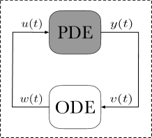
Figure 1: Interconnection between PDE-ODE models.

In this paper, the linear ODEs are of the following form:

$$\begin{split}&\dot{x}(t)=Ax(t)+Bv(t),\\ &w(t)=Cx(t).\end{split}$$ (1)

For $s\in[a,b]$, the linear one dimensional PDEs are described in the following form:

$$\dot{z}(s,t)=A_{0}(s)z(s,t)+A_{1}(s)\frac{\partial z(s,t)}{\partial s}$$ (2)

$$\qquad\qquad\qquad+A_{2}(s)\frac{\partial^{2}z(s,t)}{\partial s^{2}}+B_{1}(s)u(t),$$

$$y(t)=C_{1}z(t)+\int_{a}^{b}\left(C_{a}(s)z(s,t)+C_{b}(s)\frac{\partial z(s,t)}{\partial s}\right)\text{d}s,$$

$$B_{c}\text{col}\Big{(}z(a,t),z(b,t),\frac{\partial z(s,t)}{\partial s}\mid_{s=a},\frac{\partial z(s,t)}{\partial s}\mid_{s=b}\Big{)}=0.$$

Here, $x(t)\in\mathbb{R}^{n_{\text{o}}}$ and $z(s,t)\in\mathbb{R}^{n_{\text{p}}}$ are the states of the ODEs and the PDEs respectively. The models (1)-(2) are connected by the signals $\text{col}(v(t),w(t))\in\mathbb{R}^{m_{\text{o}}}\times\mathbb{R}^{p_{\text{o}}}$ and $\text{col}(u(t),y(t))\in\mathbb{R}^{m_{\text{p}}}\times\mathbb{R}^{p_{\text{p}}}$. In (1) $A,B,C$ are constant matrices of suitable dimensions. In (2), $A_{0}(s),A_{1}(s),A_{2}(s),B_{1}(s),C_{a}(s),C_{b}(s)$ are matrix valued functions of appropriate dimensions and $C_{1}$ is a constant matrix. $B_{c}\in\mathbb{R}^{2n_{\text{p}}\times 4n_{\text{p}}}$ is required to have full row rank.

The interconnection between (1)-(2) is described by a matrix $L\in\mathbb{R}^{{m_{\text{o}}+m_{\text{p}}}\times{p_{\text{o}}+p_{\text{p}}}}$ that has full row rank and relates the interconnection signals with the help of the following algebraic equation:

$$\left[\begin{array}[]{c}v(t)\\ u(t)\end{array}\right]=L\left[\begin{array}[]{c}w(t)\\ y(t)\end{array}\right].$$ (3)

In this paper, we develop a scalable approach to verify the stability of the coupled system in (1)-(2) that does not depend on any discretization or approximation. Regarding verifying stability, many methods used in the analysis of Distributed Parameter Systems(DPS) rely on either application-specific analytical approaches(e.g. Nicaise et al. (2009)) or projection of the entire system onto a finite-dimensional vector space as shown in Ravindran (2000), Das et al. (2018) and the references therein. Once projected to a finite-dimensional subspace, the reduced order model is treated as a set of ODEs, and there are many well-studied approaches to test for stability and design controllers. However, discretization techniques for approximating an infinite-dimensional system with a finite-dimensional model are prone to numerical instabilities and other truncation errors. This results in large system matrices which often make them computationally demanding. Moreover, these finite-dimensional approximations of the DPS do not necessarily represent the behavior of the original system to a required level of accuracy, thus the properties, such as stability, robustness are not exact if the finite dimensional approximation replaces the original model. Another approach frequently used in stabilization and control of coupled PDE-ODE systems is the backstepping method, e.g. Krstic and Smyshlyaev (2008), Krstic (2009) and Susto and Krstic (2010). The backstepping technique does not require any discretization or approximation of the model; however, it does not allow us to utilize Lyapunov theory to verify stability. Also, these methods are neither generic nor scalable for a general class of PDE-ODE coupled system.

On the other hand, using the extension of Lyapunov theory in infinite-dimensional space by Datko (1970), many attempts were made to use Sum-of-Squares (SOS) optimization methods for constructing Lyapunov functions for PDEs. Some of the notable works include but not limited to Papachristodoulou and Peet (2006), Fridman and Orlov (2009) and Valmorbida et al. (2016). However, these works cannot deal with a general class of coupled PDEs that involve reaction, transport, and diffusion terms. From our lab, numerous problems related to the analysis of stability and robustness and controller-observer synthesis are addressed in Meyer and Peet (2015), Gahlawat and Peet (2017) etc. Recently, Peet (2018), Shivakumar and Peet (2018) have developed a novel SOS framework for representation, stability and robustness analysis for coupled PDEs with arbitrary boundary condition. These results provide a unifying framework and a computationally scalable method for the analysis of a large class of PDEs.

The contributions of this paper involve extending the representation and the stability analysis of coupled PDEs to the case of linear PDE-ODE coupled systems. To this end, we construct a quadratic Lyapunov function of the form $V({x},{z})=\Big{\langle}{\begin{bmatrix}x\\ z\end{bmatrix}},{\mathcal{P}_{\tiny\{P,Q,Q^{\top},S,R_{1},R_{2}\}}\begin{bmatrix}x\\ z\end{bmatrix}}\Big{\rangle}$, where $\mathcal{P}_{\tiny\{P,Q,Q^{\top},S,R_{1},R_{2}\}}$ is a class of self-adjoint linear operator on $\mathbb{R}^{n_{\text{o}}}\times L_{2}$. The criterion for the stability of the PDE-ODE coupled system is to search for a positive $\mathcal{P}_{\{P,Q_{1},Q_{2},S,R_{1},R_{2}\}}$that restricts the time derivative of the Lyapunov function to be negative. We parametrize the multipliers and integral operators of $\mathcal{P}_{\{P,Q_{1},Q_{2},S,R_{1},R_{2}\}}$with polynomial kernels of semi-separable class as in (1). We show that the positivity constraints on these operators can be re-formulated as scalable Linear Matrix Inequalities(LMIs) that establish the stability condition for PDE-ODE coupled system.

$$\left(\mathcal{P}_{\tiny\{P,Q,Q^{\top},S,R_{1},R_{2}\}}\begin{bmatrix}x\\ z\end{bmatrix}\right)(s):=$$

$${\scriptsize\begin{bmatrix}Px+\int_{a}^{b}Q(s)z(s)ds\\ Q^{\top}(s)x+S(s)z(s)+\int_{a}^{s}R_{1}(s,\eta)z(\eta)\text{d}\eta+\int_{s}^{b}R_{2}(s,\eta)z(\eta)\text{d}\eta\end{bmatrix}}$$ (4)

The organization of the paper is as follows. Section 2 provides a preliminary discussion on the notations, a model of the PDE-ODE coupled systems and the Lyapunov stability theory. In Section 3, we define the class of operators $\mathcal{P}_{\{P,Q_{1},Q_{2},S,R_{1},R_{2}\}}$and derive its positivity condition as well as the composition and adjoint operations of these operators. In Section 4, the PDE-ODE coupled model has been represented using the same class of operators. In Section 5, the equivalent LMI conditions have been derived to verify the stability of PDE-ODE coupled system. In Section 6, we numerically illustrate the methodology to verify the stability of example PDE-ODE coupled systems in MATLAB. At last, Section 7 provides some conclusions and directions for future research.

2 Preliminaries

2.1 Notation

For convenience, we denote $\frac{\partial x}{\partial s}:=x_{s}$ and $\frac{\partial^{2}x}{\partial s^{2}}:=x_{ss}$. We use $\mathbb{Z}$ to denote a field of integers. We use $\mathbb{S}^{m}\subset\mathbb{R}^{m\times m}$ to denote the symmetric matrices. We define the space of square integrable $\mathbb{R}^{m}$-valued functions on $X$ as $L_{2}^{m}(X)$. $L_{2}^{m}(X)$ is equipped with the inner product $\langle x,y\rangle_{L_{2}}=\int_{a}^{b}x^{\top}(s)y(s)\text{d}s$. For denoting the inner product in $\mathbb{R}^{n}$, we use $\langle{x},{y}\rangle_{\mathbb{R}^{n}}=x^{\top}y$. The Sobolov space is defined by $W^{q,n}(X):=\{x\in L_{2}^{n}(X)\mid\frac{\partial^{k}x}{\partial s^{k}}\in L_{2}^{n}(X)\text{ for all }k\leq q\}$. For an inner product space $X$, operator $\mathcal{P}:X\to X$ is called positive, if for all $x\in X$, we have $\langle{x},{\mathcal{P}x}\rangle_{X}\geq 0$. We use $\mathcal{P}\succcurlyeq 0$ to indicate that $\mathcal{P}$ is a positive operator. We say that $\mathcal{P}:X\to X$ is coercive if there exists some $\epsilon>0$ such that $\langle{x},{\mathcal{P}x}\rangle_{X}\geq\epsilon\|x\|_{X}^{2}$ for all $x\in X$.

2.2 PDE-ODE Coupled System

In this section, we elaborate on the description of the coupled linear PDE-ODE system.The system is represented as an interconnection between two systems; one of them is governed by a set of partial differential equations (PDEs) while the other is governed by a set of ordinary differential equations (ODEs). In the following subsections we briefly describe the corresponding PDE and ODE model.

2.2.1 A. ODE Model:

The ODE model has the following state space representation:

$$\begin{split}\dot{x}(t)&=Ax(t)+Bv(t),\\ w(t)&=Cx(t),\end{split}$$ (5)

where $x(t)\in\mathbb{R}^{n_{\text{o}}}$ are the state variables, $v(t)\in\mathbb{R}^{m_{\text{o}}}$, $w(t)\in\mathbb{R}^{p_{\text{o}}}$ are the interconnection signals. $A,B,C$ are matrices of suitable dimensions.

2.2.2 B. PDE Model:

An operator based notation can be utilized to represent the PDE model in the following abstract state space form:

$$\begin{split}\dot{z}(t)&=\mathcal{A}z(t)+\mathcal{B}u(t),\\ y(t)&=\mathcal{C}z(t).\end{split}$$ (6)

For functions $\mathbf{z}:[a,b]\times\mathbb{R}^{+}\rightarrow\mathbb{R}^{n_{\text{p}}}$, $\mathbf{u}:\mathbb{R}^{+}\rightarrow\mathbb{R}^{m_{\text{p}}}$, $\mathbf{y}:\mathbb{R}^{+}\rightarrow\mathbb{R}^{p_{\text{p}}}$, the system operators $\mathcal{A}:L_{2}^{n_{\text{p}}}[a,b]\supset D_{\mathcal{A}}\to L_{2}^{n_{\text{p}}}[a,b],~{}\mathcal{B}:\mathbb{R}^{m_{\text{p}}}\to L_{2}^{n_{\text{p}}}[a,b]$ and $~{}\mathcal{C}:L_{2}^{n_{\text{p}}}[a,b]\to\mathbb{R}^{p_{\text{p}}}$ are specified by the following definitions:

$$(\mathcal{A}\mathbf{z})(s) :=A_{0}(s)\mathbf{z}(s)+A_{1}(s)\mathbf{z}_{s}+A_{2}(s)\mathbf{z}_{ss},$$

$$(\mathcal{B}\mathbf{u})(s) :=B_{1}(s)\mathbf{u},$$

$$\mathcal{C}\mathbf{z} :=C_{1}\mathbf{z}_{b}+\int\limits_{a}^{b}\Bigg{(}C_{a}(s)\mathbf{z}+C_{b}(s)\mathbf{z}_{s}\Bigg{)}\text{d}s,$$ (7)

with its domain

$$\begin{split}D_{\mathcal{A}}:=&\{\mathbf{z}\in W^{2,2}:B_{c}\mathbf{z}_{b}=0\},\\ \mathbf{z}_{b}:=&\text{col}\big{(}\mathbf{z}(a),\mathbf{z}(b),\mathbf{z}_{s}(a),\mathbf{z}_{s}(b)\big{)}.\end{split}$$ (8)

In (2.2.2), $A_{0}(s),A_{1}(s),A_{2}(s)\in\mathbb{R}^{n_{\text{p}}\times n_{\text{p}}}$ are matrix valued functions. $B_{1}(s)\in\mathbb{R}^{n_{\text{p}}\times m_{\text{p}}}$, $C_{a}(s),C_{b}(s)\in\mathbb{R}^{m_{\text{p}}\times n_{\text{p}}}$ are also matrix valued functions. $C_{1}\in\mathbb{R}^{m_{\text{p}}\times 4n_{\text{p}}}$ is a constant matrix. $B_{c}\in\mathbb{R}^{2n_{\text{p}}\times 4n_{\text{p}}}$ has full row rank.

2.2.3 C. PDE-ODE Interconnection:

A regular interconnection between the ODE model in (5) and the PDE model in (6) is specified by the following algebraic constraint on the variable pairs $(v,w)$ and $(u,y)$:

$$\left[\begin{array}[]{c}v(t)\\ \hline\cr u(t)\end{array}\right]=\underbrace{\left[\begin{array}[]{c|c}L_{1}&L_{2}\\ \hline\cr L_{3}&L_{4}\end{array}\right]}_{L}\left[\begin{array}[]{c}w(t)\\ \hline\cr y(t)\end{array}\right].$$ (9)

The matrix $L\in\mathbb{R}^{{m_{\text{o}}+m_{\text{p}}}\times{p_{\text{o}}+p_{\text{p}}}}$ has full row rank and is partitioned to relate interconnection signals of ODEs and PDEs individually. Substituting (9) in (5) and (6), we obtain the following autonomous state-space model.

$$\begin{bmatrix}\dot{\mathbf{x}}(t)\\ \dot{\mathbf{z}}(t)\end{bmatrix}=\underbrace{\begin{bmatrix}A+BL_{1}C&BL_{2}\mathcal{C}\\ \mathcal{B}L_{3}C&\mathcal{A}+\mathcal{B}L_{4}\mathcal{C}\end{bmatrix}}_{\bar{\mathbf{A}}}\begin{bmatrix}\mathbf{x}(t)\\ \mathbf{z}(t)\end{bmatrix},$$ (10)

with $\bar{\mathbf{A}}:\mathbb{R}^{n_{\text{o}}}\times L_{2}^{n_{\text{p}}}[a,b]\supset\mathbb{R}^{n_{\text{o}}}\times D_{\mathcal{A}}\rightarrow\mathbb{R}^{n_{\text{o}}}\times L_{2}^{n_{\text{p}}}[a,b]$. We define $X:=\mathbb{R}^{n_{\text{o}}}\times L_{2}^{n_{\text{p}}}[a,b]$ with inner product

$$\Bigg{\langle}\begin{bmatrix}x_{1}\\ x_{2}(s)\end{bmatrix},\begin{bmatrix}z_{1}\\ z_{2}(s)\end{bmatrix}\Bigg{\rangle}_{X}:=x_{1}^{\top}z_{1}+\big{\langle}x_{2},z_{2}\big{\rangle}_{L_{2}^{n_{\text{p}}}[a,b]},$$ (11)

and norm

$$\Bigg{\lvert}\Bigg{\lvert}\begin{bmatrix}x_{1}\\ x_{2}(s)\end{bmatrix}\Bigg{\rvert}\Bigg{\rvert}_{X}^{2}=\mid\mid x_{1}\mid\mid_{\mathbb{R}^{n_{\text{o}}}}^{2}+\mid\mid x_{2}(s)\mid\mid_{L_{2}^{n_{\text{p}}}[a,b]}^{2}.$$ (12)

2.3 Lyapunov Stability Theorem

The necessary and sufficient condition for exponential stability of a linear infinite dimensional system has been provided in Curtain and Zwart (1995). The same can be extended as Theorem 1 that provides a condition to verify the exponential stability of PDE-ODE coupled system.

Theorem 1

Suppose $\bar{\mathbf{A}}:X\supset\mathbb{R}^{n_{\text{o}}}\times D_{\mathcal{A}}\rightarrow X$ generates a strongly continuous semigroup and there exists $\alpha,\beta,\gamma>0$ and $\mathcal{P}:X\to X$ such that

$$\alpha\Bigg{\lvert}\Bigg{\lvert}\begin{bmatrix}x\\ z\end{bmatrix}\Bigg{\rvert}\Bigg{\rvert}_{X}^{2}\leq\Bigg{\langle}\begin{bmatrix}x\\ z\end{bmatrix},{\mathcal{P}\begin{bmatrix}x\\ z\end{bmatrix}}\Bigg{\rangle}_{X}\leq\beta\Bigg{\lvert}\Bigg{\lvert}\begin{bmatrix}x\\ z\end{bmatrix}\Bigg{\rvert}\Bigg{\rvert}_{X}^{2},$$

and

$$\Bigg{\langle}\begin{bmatrix}x\\ z\end{bmatrix},{\mathcal{P}\bar{\mathbf{A}}\begin{bmatrix}x\\ z\end{bmatrix}}\Bigg{\rangle}_{X}+\Bigg{\langle}\bar{\mathbf{A}}\begin{bmatrix}x\\ z\end{bmatrix},{\mathcal{P}\begin{bmatrix}x\\ z\end{bmatrix}}\Bigg{\rangle}_{X}\leq-\gamma\Bigg{\lvert}\Bigg{\lvert}\begin{bmatrix}x\\ z\end{bmatrix}\Bigg{\rvert}\Bigg{\rvert}_{X}^{2},$$ (13)

for all $x\in\mathbb{R}^{n_{\text{o}}}$, $z\in D_{\mathcal{A}}$. Then (10) is exponentially stable.

3 Parametrization of the Class of Operator $\mathcal{P}_{\{P,Q_{1},Q_{2},S,R_{1},R_{2}\}}$

Definition 2

For a matrix $P\in\mathbb{R}^{n_{\text{o}}\times n_{\text{o}}}$, and bounded polynomial functions $Q_{1}:[a,b]\rightarrow\mathbb{R}^{n_{\text{o}}\times n_{\text{p}}}$, $Q_{2}:[a,b]\rightarrow\mathbb{R}^{n_{\text{p}}\times n_{\text{o}}}$, $S:[a,b]\rightarrow\mathbb{R}^{n_{\text{p}}\times n_{\text{p}}}$, and $R_{1},R_{2}:[a,b]\times[a,b]\rightarrow\mathbb{R}^{n_{\text{p}}\times n_{\text{p}}}$ with $x\in\mathbb{R}^{n_{\text{o}}}$ and $z\in L_{2}^{n_{\text{p}}}[a,b]$, the class of operators $\mathcal{P}_{\{P,Q_{1},Q_{2},S,R_{1},R_{2}\}}$are defined as

$$\left(\mathcal{P}_{\{P,Q_{1},Q_{2},S,R_{1},R_{2}\}}\begin{bmatrix}x\\ z\end{bmatrix}\right)(s):=$$

$${\scriptsize\begin{bmatrix}Px+\int_{a}^{b}Q_{1}(s)z(s)ds\\ Q_{2}(s)x+S(s)z(s)+\int_{a}^{s}R_{1}(s,\eta)z(\eta)\text{d}\eta+\int_{s}^{b}R_{2}(s,\eta)z(\eta)\text{d}\eta\end{bmatrix}}.$$ (14)

In the remainder of this section, we investigate three properties of the class of operator $\mathcal{P}_{\{P,Q_{1},Q_{2},S,R_{1},R_{2}\}}$. First, we provide a sufficient condition on the positivity of the operator. Subsequently, an efficient method to compute composition and adjoint of the operators of the form $\mathcal{P}_{\{P,Q_{1},Q_{2},S,R_{1},R_{2}\}}$has been provided. The composition and the adjoint operation on the operators will allow us to obtain a scalable represention of the PDE-ODE coupled system. With the help of the positivity condition on the operator, the Lyapunov stability conditions can be reformulated as LMIs.

3.1 Positivity of $\mathcal{P}_{\tiny\{P,Q,Q^{\top},S,R_{1},R_{2}\}}$ Operator

Theorem 3

For any functions $Z(s)\in\mathbb{R}^{d_{1}\times n}$, $Z(s,\eta)\in\mathbb{R}^{d_{2}\times n}$ $\forall s,\eta\in[a,b]$, suppose there exists a matrix $T\succcurlyeq 0$ such that

$$P =T_{11},$$

$$Q(s) =T_{12}Z(s)+\int_{s}^{b}T_{13}Z(\eta,s)\text{d}\eta+\int_{a}^{s}T_{14}Z(\eta,s)\text{d}\eta,$$

$$S(s) =Z^{\top}(s)T_{22}Z(s),$$

$$R_{1}(s,\eta) =Z^{\top}(s)T_{23}Z(s,\eta)+Z^{\top}(\eta,s)T_{42}Z^{\top}(\eta)$$

$$+\int_{s}^{b}Z^{\top}(\theta,s)T_{33}Z(\theta,\eta)\text{d}\theta+\int_{\eta}^{s}Z^{\top}(\theta,s)T_{43}Z(\theta,\eta)\text{d}\theta$$

$$+\int_{a}^{\eta}Z^{\top}(\theta,s)T_{44}Z(\theta,\eta)\text{d}\theta,$$

$$R_{2}(s,\eta) =Z^{\top}(s)T_{32}Z(s,\eta)+Z^{\top}(\eta,s)T_{24}Z^{\top}(\eta)$$

$$+\int_{\eta}^{b}Z^{\top}(\theta,s)T_{33}Z(\theta,\eta)\text{d}\theta+\int_{s}^{\eta}Z^{\top}(\theta,s)T_{34}Z(\theta,\eta)\text{d}\theta$$

$$+\int_{a}^{s}Z^{\top}(\theta,s)T_{44}Z(\theta,\eta)\text{d}\theta,$$ (15)

with

$$T=\begin{bmatrix}T_{11}&T_{12}&T_{13}&T_{14}\\ T_{21}&T_{22}&T_{23}&T_{24}\\ T_{31}&T_{32}&T_{33}&T_{34}\\ T_{41}&T_{42}&T_{43}&T_{44}\end{bmatrix}.$$

Then the operator $\mathcal{P}_{\tiny\{P,Q,Q^{\top},S,R_{1},R_{2}\}}$  as defined in (2) is positive, i.e. $\mathcal{P}_{\tiny\{P,Q,Q^{\top},S,R_{1},R_{2}\}}\succcurlyeq 0$.

Since $T\succcurlyeq 0$, we can define a square root of $T$ as $U=\begin{bmatrix}U_{1}&U_{2}&U_{3}&U_{4}\end{bmatrix}$.

$$T=\begin{bmatrix}T_{11}&T_{12}&T_{13}&T_{14}\\ T_{21}&T_{22}&T_{23}&T_{24}\\ T_{31}&T_{32}&T_{33}&T_{34}\\ T_{41}&T_{42}&T_{43}&T_{44}\end{bmatrix} =U^{\top}U$$

$$=\begin{bmatrix}U_{1}^{\top}U_{1}&U_{1}^{\top}U_{2}&U_{1}^{\top}U_{3}&U_{1}^{\top}U_{4}\\ *^{\top}&U_{2}^{\top}U_{2}&U_{2}^{\top}U_{3}&U_{2}^{\top}U_{4}\\ *^{\top}&*^{\top}&U_{3}^{\top}U_{3}&U_{3}^{\top}U_{4}\\ *^{\top}&*^{\top}&*^{\top}&U_{4}^{\top}U_{4}\end{bmatrix}$$

For $x_{1}\in\mathbb{R}^{m}$ and $x_{2}\in L_{2}^{n}[a,b]$, let us define $v(s):=U_{1}x_{1}+(\Psi x_{2})(s)$, where

$$(\Psi x_{2})(s) =U_{2}Z(s)+\int_{a}^{s}U_{3}Z(s,\eta)x_{2}(\eta)\text{d}\eta$$

$$\quad+\int_{s}^{b}U_{4}Z(s,\eta)x_{2}(\eta)\text{d}\eta.$$

Then

$$\Big{\langle}{v(s)},{v(s)}\Big{\rangle}_{\mathbb{R}^{m}\times L_{2}^{n}[a,b]}$$

$$=\langle{U_{1}x_{1}},{U_{1}x_{1}}\rangle_{\mathbb{R}^{m}}+\langle{U_{1}x_{1}},{(\Psi x_{2})(s)}\rangle_{\mathbb{R}^{m}}$$

$$~{}~{}~{}+\langle{(\Psi x_{2})(s)},{U_{1}x_{1}}\rangle_{L_{2}^{n}[a,b]}+\langle{(\Psi x_{2})(s)},{(\Psi x_{2})(s)}\rangle_{L_{2}^{n}[a,b]}$$

$$\quad=\Big{\langle}{\begin{bmatrix}x_{1}\\ x_{2}\end{bmatrix}}{\mathcal{P}_{\tiny\{P,Q,Q^{\top},S,R_{1},R_{2}\}},\begin{bmatrix}x_{1}\\ x_{2}\end{bmatrix}}\Big{\rangle}_{\mathbb{R}^{m}\times L_{2}^{n}[a,b]}\geq 0.$$

Hence $\mathcal{P}_{\tiny\{P,Q,Q^{\top},S,R_{1},R_{2}\}}\succcurlyeq 0$.  

3.2 Composition of The Operators

In this subsection, we show that the composition of two operators of the class $\mathcal{P}_{\{P,Q_{1},Q_{2},S,R_{1},R_{2}\}}$also takes the same structure and provide an efficient method to calculate it.

Lemma 4

For any matrices $A,P\in\mathbb{R}^{m\times m}$ and bounded functions $B_{1},Q_{1}:[a,b]\to\mathbb{R}^{m\times n}$, $B_{2},Q_{2}:[a,b]\to\mathbb{R}^{n\times m}$, $D,S:[a,b]\to\mathbb{R}^{n\times n}$, $C_{i},R_{i}:[a,b]\times[a,b]\to\mathbb{R}^{n\times n}$ with $i\in\{1,2\}$, the following identity holds

$$\mathcal{P}_{\tiny\{A,B_{1},B_{2},D,C_{1},C_{2}\}} \mathcal{P}_{\tiny\{P,Q_{1},Q_{2},S,R_{1},R_{2}\}}$$

$$=\mathcal{P}_{\{\hat{P},\hat{Q}_{1},\hat{Q}_{2},\hat{S},\hat{R}_{1},\hat{R}_{2}\}},$$ (16)

where

$$\hat{P} =AP+\int_{a}^{b}B_{1}(s)Q_{2}(s)\text{d}s,$$

$$\hat{Q}_{1}(s) =AQ_{1}(s)+B_{1}(s)S(s)+\int_{s}^{b}B_{1}(\eta)R_{1}(\eta,s)\text{d}\eta$$

$$\qquad+\int_{a}^{s}B_{1}(\eta)R_{2}(\eta,s)\text{d}\eta,$$

$$\hat{Q}_{2}(s) =B_{2}(s)P+D(s)Q_{2}(s)+\int_{a}^{s}C_{1}(s,\eta)Q_{2}(\eta)\text{d}\eta$$

$$\qquad+\int_{s}^{b}C_{2}(s,\eta)Q_{2}(\eta)\text{d}\eta,$$

$$\hat{S}(s) =D(s)S(s),$$

$$\hat{R}_{1}(s,\eta) =B_{2}(s)Q_{1}(\eta)+D(s)R_{1}(s,\eta)+C_{1}(s,\eta)S(\eta)$$

$$+\int_{a}^{\eta}C_{1}(s,\theta)R_{2}(\theta,\eta)\text{d}\theta+\int_{\eta}^{s}C_{1}(s,\theta)R_{1}(\theta,\eta)\text{d}\theta$$

$$+\int_{s}^{b}C_{2}(s,\theta)R_{1}(\theta,\eta)\text{d}\theta,$$

$$\hat{R}_{2}(s,\eta) =B_{2}(s)Q_{1}(\eta)+D(s)R_{2}(s,\eta)+C_{2}(s,\eta)S(\eta)$$

$$+\int_{a}^{s}C_{1}(s,\theta)R_{2}(\theta,\eta)\text{d}\theta+\int_{s}^{\eta}C_{2}(s,\theta)R_{2}(\theta,\eta)\text{d}\theta$$

$$+\int_{\eta}^{b}C_{2}(s,\theta)R_{1}(\theta,\eta)\text{d}\theta.$$ (17)

The proof can be found in the Appendix C.   For convenience, we say

$$\Big{(}\hat{P},\hat{Q}_{1},\hat{Q}_{2},\hat{S},\hat{R}_{1},\hat{R}_{2}\Big{)}= \Big{(}A,B_{1},B_{2},D,C_{1},C_{2}\Big{)}$$ (18)

$$\times\Big{(}P,Q_{1},Q_{2},S,R_{1},R_{2}\Big{)},$$ (19)

if $\hat{P},\hat{Q}_{1},\hat{Q}_{2},\hat{S},\hat{R}_{1},\hat{R}_{2}$ are related to $A,B_{1},B_{2},D,C_{1},C_{2}$ and $P,Q_{1},Q_{2},S,R_{1},R_{2}$ according to (4) in Lemma 4.

3.3 Adjoint of The Operators

Now, we also discuss the adjoint of an operator of the class $\mathcal{P}_{\{P,Q_{1},Q_{2},S,R_{1},R_{2}\}}$and it is typically denoted by $\mathcal{P}_{\{P,Q_{1},Q_{2},S,R_{1},R_{2}\}}^{*}$.

Lemma 5

For any matrices $P\in\mathbb{R}^{m\times m}$ and bounded functions $Q_{1}:[a,b]\to\mathbb{R}^{m\times n}$, $Q_{2}:[a,b]\to\mathbb{R}^{n\times m}$, $S:[a,b]\to\mathbb{R}^{n\times n}$, $R_{1},R_{2}:[a,b]\times[a,b]\to\mathbb{R}^{n\times n}$, the following identity holds for any $x\in\mathbb{R}^{m},y\in L_{2}^{n}([a,b])$.

$$\Big{\langle}{x},{\mathcal{P}_{\tiny\{P,Q_{1},Q_{2},S,R_{1},R_{2}\}}y}\Big{\rangle}_{\mathbb{R}^{m}\times L_{2}^{n}[a,b]}$$

$$=\Big{\langle}{\mathcal{P}_{\tiny\{P,Q_{1},Q_{2},S,R_{1},R_{2}\}}^{*}x},{y}\Big{\rangle}_{\mathbb{R}^{m}\times L_{2}^{n}[a,b]},$$ (20)

where, $\mathcal{P}_{\tiny\{P,Q_{1},Q_{2},S,R_{1},R_{2}\}}^{*}=\mathcal{P}_{\tiny\{\hat{P},\hat{Q}_{1},\hat{Q}_{2},\hat{S},\hat{R}_{1},\hat{R}_{2}\}}$ with

$$\hat{P}=P^{\top}, \hat{S}(s)=S^{\top}(s),$$

$$\hat{Q}_{1}(s)=Q_{2}^{\top}(s), \hat{R}_{1}(s,\eta)=R_{2}^{\top}(\eta,s),$$

$$\hat{Q}_{2}(s)=Q_{1}^{\top}(s), \hat{R}_{2}(s,\eta)=R_{1}^{\top}(\eta,s).$$ (21)

The proof can be found in the Appendix D.   For convenience, we say

$$\Big{(}\hat{P},\hat{Q}_{1},\hat{Q}_{2},\hat{S},\hat{R}_{1},\hat{R}_{2}\Big{)}=\ \Big{(}P,Q_{1},Q_{2},S,R_{1},R_{2}\Big{)}^{*},$$ (22)

if $\hat{P},\hat{Q}_{1},\hat{Q}_{2},\hat{S},\hat{R}_{1},\hat{R}_{2}$ are related to $P,Q_{1},Q_{2},S,R_{1},R_{2}$ according to (5) in Lemma 5.

4 Fundamental Identities

In this section, we utilize the class of operators defined by $\mathcal{P}_{\{P,Q_{1},Q_{2},S,R_{1},R_{2}\}}$to uniquely represent the system (10) in terms of the variables $\mathbf{x}$ and $\mathbf{z}_{ss}$ replacing $\mathbf{z}$.

Lemma 6

Suppose $\mathbf{x}\in\mathbb{R}^{n_{\text{o}}}$ and $\mathbf{z}\in W^{2,2}[a,b]$ and

$$B_{c}\text{col}(\mathbf{z}(a),\mathbf{z}(b),\mathbf{z}_{s}(a),\mathbf{z}_{s}(b))=0,$$

with $B_{c}\in\mathbb{R}^{2n_{\text{p}}\times 4n_{\text{p}}}$ has full row rank. Then

$$\begin{bmatrix}\mathbf{x}\\ \mathbf{z}\end{bmatrix}=\mathcal{P}_{\{I,0,0,0,G_{1},G_{2}\}}\begin{bmatrix}\mathbf{x}\\ \mathbf{z}_{ss}\end{bmatrix},$$ (23)

$$\begin{bmatrix}\mathbf{x}\\ \mathbf{z}_{s}\end{bmatrix}=\mathcal{P}_{\{I,0,0,0,G_{3},G_{4}\}}\begin{bmatrix}\mathbf{x}\\ \mathbf{z}_{ss}\end{bmatrix},$$ (24)

with

$$G_{1}(s,\eta) =B_{a}(s,\eta)+(s-\eta)I,$$ (25)

$$G_{2}(s,\eta) =B_{a}(s,\eta),$$ (26)

$$G_{3}(s,\eta) =B_{b}(s,\eta)+I,$$ (27)

$$G_{4}(s,\eta) =B_{b}(s,\eta),$$ (28)

$$B_{a}(s,\eta) =-\begin{bmatrix}I&(s-a)I\end{bmatrix}B_{f}(\eta),$$ (29)

$$B_{b}(\eta) =-\begin{bmatrix}0&I\end{bmatrix}B_{f}(\eta),$$ (30)

$$B_{f}(\eta) =(B_{c}B_{d})^{-1}B_{c}\begin{bmatrix}0\\ (b-\eta)I\\ 0\\ I\end{bmatrix},$$ (31)

$$B_{d} =\begin{bmatrix}I&0\\ I&(b-a)I\\ 0&I\\ 0&I\end{bmatrix}.$$ (32)

For detailed proof, we refer to (Peet, 2018, p. 2-3).  

Lemma 7

Suppose $\mathbf{x}\in\mathbb{R}^{n_{\text{o}}}$ and $\mathbf{z}\in W^{2,2}[a,b]$ and

$$B_{c}\ \text{col}(\mathbf{z}(a),\mathbf{z}(b),\mathbf{z}_{s}(a),\mathbf{z}_{s}(b))=0,$$

with $B_{c}\in\mathbb{R}^{2n_{\text{p}}\times 4n_{\text{p}}}$ has full row rank. Then

$$\begin{bmatrix}\dot{\mathbf{x}}\\ \dot{\mathbf{z}}\end{bmatrix}=\begin{bmatrix}A+BL_{1}C&BL_{2}\mathcal{C}\\ \mathcal{B}L_{3}C&\mathcal{A}+\mathcal{B}L_{4}\mathcal{C}\end{bmatrix}\begin{bmatrix}\mathbf{x}\\ \mathbf{z}\end{bmatrix}$$ (33)

implies

$$\begin{bmatrix}\dot{\mathbf{x}}\\ \dot{\mathbf{z}}\end{bmatrix}=\mathcal{P}_{\{U,V_{1},V_{2},Y,W_{1},W_{2}\}}\begin{bmatrix}\mathbf{x}\\ {\mathbf{z}}_{ss}\end{bmatrix},$$ (34)

where

$$U=\Lambda_{1}+\Lambda_{2}, Y=\Pi_{1}+\Pi_{2}+A_{2}+B_{1}L_{4}C_{3},$$

$$V_{1}=\Omega_{1}+\Omega_{2}+BL_{2}C_{3}, W_{1}=\Psi_{1}+\Psi_{2},$$

$$V_{2}=\Sigma_{1}+\Sigma_{2}, W_{2}=\Upsilon_{1}+\Upsilon_{2},$$

with

$$\big{(}\Lambda_{1},\Omega_{1},\Sigma_{1},\Pi_{1},\Psi_{1},\Upsilon_{1}\big{)}$$

$$=\big{(}A+BL_{1}C,BL_{2}C_{a},B_{1}L_{3}C,A_{0}+B_{1}L_{4}C_{a},0,0\big{)}$$

$$\quad\qquad\times\big{(}I,0,0,0,G_{1},G_{2}\big{)},$$

$$\big{(}\Lambda_{2},\Omega_{2},\Sigma_{2},\Pi_{2},\Psi_{2},\Upsilon_{2}\big{)}$$

$$=\big{(}0,BL_{2}C_{b},0,A_{1}+B_{1}L_{4}C_{b},0,0\big{)}\times\big{(}I,0,0,0,G_{3},G_{4}\big{)},$$

$$C_{3}(s)=-C_{1}B_{d}B_{c}(s)+C_{1}\begin{bmatrix}0\\ (b-s)I\\ 0\\ I\end{bmatrix}.$$ (35)

Moreover, the definitions of $G_{1},G_{2},G_{3},G_{4}$ are given according to Lemma 6.

For detailed proof, see Appendix A.   The above identities imply that the original state $\mathbf{z}$ can be fully reconstructed by the ’fundamental state’ $\mathbf{z}_{ss}$ (see Peet (2018)). Moreover, the new representation of the system dynamics in terms of $\mathbf{z}_{ss}$ is independent of the boundary constraints. In the subsequent sections, these identities are utilized for deriving stability conditions.

5 Lyapunov Stability Condition

In order to verify the stability of the PDE-ODE coupled system, we have proposed a Lyapunov function of the form

$$V(\mathbf{x},\mathbf{z})=\Bigg{\langle}\begin{bmatrix}\mathbf{x}\\ \mathbf{z}\end{bmatrix},\mathcal{P}_{\{P,Q,Q^{\top},S,R_{1},R_{2}\}}\begin{bmatrix}\mathbf{x}\\ \mathbf{z}\end{bmatrix}\Bigg{\rangle}_{X},$$ (36)

such that $\mathcal{P}_{\{P,Q,Q^{\top},S,R_{1},R_{2}\}}$ is self-adjoint, i.e.,

$$\mathcal{P}_{\{P,Q,Q^{\top},S,R_{1},R_{2}\}}=\mathcal{P}_{\{P,Q,Q^{\top},S,R_{1},R_{2}\}}^{*}.$$

5.1 Derivative of The Lyapunov Function

Theorem 8

Suppose $\mathbf{x}\in\mathbb{R}^{n_{\text{o}}}$ and $\mathbf{z}\in W^{2,2}[a,b]$ and

$$B_{c}\ \text{col}(\mathbf{z}(a),\mathbf{z}(b),\mathbf{z}_{s}(a),\mathbf{z}_{s}(b))=0,$$

with $B_{c}\in\mathbb{R}^{2n_{\text{p}}\times 4n_{\text{p}}}$ has full row rank. Moreover, suppose there exists a matrix $P\in\mathbb{R}^{n_{\text{o}}\times n_{\text{o}}}$, and bounded polynomial functions $Q:[a,b]\rightarrow\mathbb{R}^{n_{\text{o}}\times n_{\text{p}}}$, $S:[a,b]\rightarrow\mathbb{R}^{n_{\text{p}}\times n_{\text{p}}}$, $R_{1},R_{2}:[a,b]\times[a,b]\rightarrow\mathbb{R}^{n_{\text{p}}\times n_{\text{p}}}$, and

$$\bar{\mathbf{A}}=\begin{bmatrix}A+BL_{1}C&BL_{2}\mathcal{C}\\ \mathcal{B}L_{3}C&\mathcal{A}+\mathcal{B}L_{4}\mathcal{C}\end{bmatrix}.$$ (37)

Then

$$\Bigg{\langle}\begin{bmatrix}\mathbf{x}\\ \mathbf{z}\end{bmatrix},{\mathcal{P}_{\{P,Q,Q^{\top},S,R_{1},R_{2}\}}\bar{\mathbf{A}}\begin{bmatrix}\mathbf{x}\\ \mathbf{z}\end{bmatrix}}\Bigg{\rangle}_{X}$$ (38)

$$+\Bigg{\langle}\bar{\mathbf{A}}\begin{bmatrix}\mathbf{x}\\ \mathbf{z}\end{bmatrix},{\mathcal{P}_{\{P,Q,Q^{\top},S,R_{1},R_{2}\}}\begin{bmatrix}\mathbf{x}\\ \mathbf{z}\end{bmatrix}}\Bigg{\rangle}_{X}$$

$$=\Bigg{\langle}\begin{bmatrix}\mathbf{x}\\ {\mathbf{z}}_{ss}\end{bmatrix},\mathcal{P}_{\{\hat{K},\hat{L},\hat{L}^{\top},\hat{M},\hat{N}_{1},\hat{N}_{2}\}}\begin{bmatrix}\mathbf{x}\\ {\mathbf{z}}_{ss}\end{bmatrix}\Bigg{\rangle}_{X}$$

where

$$\hat{K}=K+\bar{K}, \hat{M}=M+\bar{M}, \quad\hat{L}=L_{1}+\bar{L}_{1},$$

$$\hat{L}^{\top}=L_{2}+\bar{L}_{2}, \hat{N}_{1}=N_{1}+\bar{N}_{1}, \quad\hat{N}_{2}=N_{2}+\bar{N}_{2},$$

$$\big{(}\bar{K},\bar{L}_{1},\bar{L}_{2},\bar{M},\bar{N}_{1},\bar{N}_{2}\big{)}= \big{(}K,L_{1},L_{2},M,N_{1},N_{2}\big{)}^{*},$$

$$\big{(}K,L_{1},L_{2},M,N_{1},N_{2}\big{)}= \big{(}I,0,0,0,G_{1},G_{2}\big{)}^{*}$$

$$\times\big{(}P,Q,Q^{\top},S,R_{1},R_{2}\big{)}$$

$$\times\big{(}U_{1},V_{1},V_{2},Y,W_{1},W_{2}\big{)}.$$ (39)

Moreover, $G_{1},G_{2}$ are as defined in Lemma 6 and $U$, $V_{1}$, $V_{2}$, $Y$, $W_{1}$, $W_{2}$ are as defined in Lemma 7.

The proof of Theorem 8 can be easily shown by substituting Lemma 6-7 in (38).  

5.2 Conditions of Exponential Stability

In order to verify the exponential stability of the PDE-ODE coupled system, we search for the operator

$$\mathcal{P}_{\{P,Q,Q^{\top},S,R_{1},R_{2}\}}\succ 0,\text{subject to}\ \mathcal{P}_{\{\hat{K},\hat{L},\hat{L}^{\top},\hat{M},\hat{N}_{1},\hat{N}_{2}\}}\prec 0.$$

Definition 9

The cone of positive operators $\mathcal{P}$ that are given in the Definition 2 with polynomial multipliers and kernels associated with degree $d_{1}$ and $d_{2}$ are specified by

$$\Phi_{d_{1},d_{2}}:=\{(P,Q,Q^{\top},S,R_{1},R_{2}):$$

the positivity condition is satisfied

$$\quad\text{according to Theorem \ref{th:positivity}}\}.$$ (40)

Theorem 10

Suppose there exists $\epsilon>0,d_{1},d_{2}\in\mathbb{Z}$ with $P\in\mathbb{R}^{n_{\text{o}}}$, and bounded polynomial functions $Q:[a,b]\rightarrow\mathbb{R}^{n_{\text{o}}\times n_{\text{p}}}$, $S:[a,b]\rightarrow\mathbb{R}^{n_{\text{p}}\times n_{\text{p}}}$, $R_{1},R_{2}:[a,b]\times[a,b]\rightarrow\mathbb{R}^{n_{\text{p}}\times n_{\text{p}}}$ such that

$$\big{(}P-\epsilon I,Q,Q^{\top},S-\epsilon I,R_{1},R_{2}\big{)}\in\Phi_{d_{1},d_{2}},$$

$$-\big{(}\hat{K},\hat{L},\hat{L}^{\top},M,N_{1},N_{2}\big{)}-\epsilon\big{(}I,0,0,0,T_{1},T_{2}\big{)}\in\Phi_{d_{1},d_{2}},$$ (41)

with

$$\hat{K}=K+\bar{K}, \hat{M}=M+\bar{M}, \quad\hat{L}=L_{1}+\bar{L}_{1},$$

$$\hat{L}^{\top}=L_{2}+\bar{L}_{2}, \hat{N}_{1}=N_{1}+\bar{N}_{1}, \quad\hat{N}_{2}=N_{2}+\bar{N}_{2},$$

$$\big{(}\bar{K},\bar{L}_{1},\bar{L}_{2},\bar{M},\bar{N}_{1},\bar{N}_{2}\big{)}= \big{(}K,L_{1},L_{2},M,N_{1},N_{2}\big{)}^{*},$$

$$\big{(}K,L_{1},L_{2},M,N_{1},N_{2}\big{)}= \big{(}I,0,0,0,G_{1},G_{2}\big{)}^{*}$$

$$\times\big{(}P,Q,Q^{\top},S,R_{1},R_{2}\big{)}$$

$$\times\big{(}U_{1},V_{1},V_{2},Y,W_{1},W_{2}\big{)},$$

$$\big{(}I,0,0,0,T_{1},T_{2}\big{)}= \big{(}I,0,0,0,G_{1},G_{2}\big{)}^{*}$$

$$\times\big{(}I,0,0,0,G_{1},G_{2}\big{)},$$ (42)

where $G_{1},G_{2}$ are as defined in Lemma 6 and $U$, $V_{1}$, $V_{2}$, $Y$, $W_{1}$, $W_{2}$ are as defined in Lemma 7. Then the system in (10) is exponentially stable.

We have defined the Lyapunov function as

$$\begin{split}V(\mathbf{x},\mathbf{z})=&\Bigg{\langle}\begin{bmatrix}\mathbf{x}\\ \mathbf{z}\end{bmatrix},\mathcal{P}_{\{P,Q,Q^{\top},S,R_{1},R_{2}\}}\begin{bmatrix}\mathbf{x}\\ \mathbf{z}\end{bmatrix}\Bigg{\rangle}_{X}\\ =&\Bigg{\langle}\begin{bmatrix}\mathbf{x}\\ \mathbf{z}\end{bmatrix},\mathcal{P}_{\{P-\epsilon I,Q,Q^{\top},S-\epsilon I,R_{1},R_{2}\}}\begin{bmatrix}\mathbf{x}\\ \mathbf{z}\end{bmatrix}\Bigg{\rangle}_{X}\\ &+\epsilon\Bigg{\lvert}\Bigg{\lvert}\begin{bmatrix}\mathbf{x}\\ \mathbf{z}\end{bmatrix}\Bigg{\rvert}\Bigg{\rvert}_{X}^{2}\geq\epsilon\Bigg{\lvert}\Bigg{\lvert}\begin{bmatrix}\mathbf{x}\\ \mathbf{z}\end{bmatrix}\Bigg{\rvert}\Bigg{\rvert}_{X}^{2}.\end{split}$$ (43)

This shows the strict positivity of $\mathcal{P}_{\tiny\{P,Q,Q^{\top},S,R_{1},R_{2}\}}$. Furthermore, based on Theorem 8, the exponential stability in Theorem 1 can be reformulated as

$$\begin{split}&\Bigg{\langle}\begin{bmatrix}\mathbf{x}\\ {\mathbf{z}}_{ss}\end{bmatrix},\mathcal{P}_{\{\hat{K},\hat{L},\hat{L}^{\top},\hat{N}_{1},\hat{N}_{2}\}}\begin{bmatrix}\mathbf{x}\\ {\mathbf{z}}_{ss}\end{bmatrix}\Bigg{\rangle}_{X}\\ =&\Bigg{\langle}\begin{bmatrix}\mathbf{x}\\ {\mathbf{z}}_{ss}\end{bmatrix},\mathcal{P}_{\{\hat{K},\hat{L},\hat{L}^{\top},\hat{N}_{1},\hat{N}_{2}\}}\begin{bmatrix}\mathbf{x}\\ {\mathbf{z}}_{ss}\end{bmatrix}\Bigg{\rangle}_{X}\\ &+\epsilon\Bigg{\lvert}\Bigg{\lvert}\begin{bmatrix}\mathbf{x}\\ \mathbf{z}\end{bmatrix}\Bigg{\rvert}\Bigg{\rvert}_{X}^{2}-\epsilon\Bigg{\lvert}\Bigg{\lvert}\begin{bmatrix}\mathbf{x}\\ \mathbf{z}\end{bmatrix}\Bigg{\rvert}\Bigg{\rvert}_{X}^{2}\\ =&\Bigg{\langle}\begin{bmatrix}\mathbf{x}\\ {\mathbf{z}}_{ss}\end{bmatrix},\mathcal{P}_{\{\hat{K},\hat{L},\hat{L}^{\top},\hat{N}_{1},\hat{N}_{2}\}}\begin{bmatrix}\mathbf{x}\\ {\mathbf{z}}_{ss}\end{bmatrix}\Bigg{\rangle}_{X}\\ +&\epsilon\Bigg{\langle}\mathcal{P}_{\{I,0,0,0,G_{1},G_{2}\}}\begin{bmatrix}\mathbf{x}\\ {\mathbf{z}}_{ss}\end{bmatrix},\mathcal{P}_{\{I,0,0,0,G_{1},G_{2}\}}\begin{bmatrix}\mathbf{x}\\ {\mathbf{z}}_{ss}\end{bmatrix}\Bigg{\rangle}_{X}\\ &-\epsilon\Bigg{\lvert}\Bigg{\lvert}\begin{bmatrix}\mathbf{x}\\ \mathbf{z}\end{bmatrix}\Bigg{\rvert}\Bigg{\rvert}_{X}^{2},\\ =&\Bigg{\langle}\begin{bmatrix}\mathbf{x}\\ {\mathbf{z}}_{ss}\end{bmatrix},\mathcal{P}_{\{\hat{K},\hat{L}_{1},\hat{L}_{2},\hat{M},\hat{N}_{1},\hat{N}_{2}\}}\begin{bmatrix}\mathbf{x}\\ {\mathbf{z}}_{ss}\end{bmatrix}\Bigg{\rangle}_{X}\\ +&\epsilon\Bigg{\langle}\begin{bmatrix}\mathbf{x}\\ {\mathbf{z}}_{ss}\end{bmatrix},\mathcal{P}_{\{I,0,0,0,T_{1},T_{2}\}}\begin{bmatrix}\mathbf{x}\\ {\mathbf{z}}_{ss}\end{bmatrix}\Bigg{\rangle}_{X}-\epsilon\Bigg{\lvert}\Bigg{\lvert}\begin{bmatrix}\mathbf{x}\\ \mathbf{z}\end{bmatrix}\Bigg{\rvert}\Bigg{\rvert}_{X}^{2}\\ &\leq-\epsilon\Bigg{\lvert}\Bigg{\lvert}\begin{bmatrix}\mathbf{x}\\ \mathbf{z}\end{bmatrix}\Bigg{\rvert}\Bigg{\rvert}_{X}^{2}.\end{split}$$

This proves the exponential stability according to Theorem 1.   In Theorem 3, we can choose $Z(s)$ to be a vector of monomials of degree $d_{1}$ and $Z(s,\eta)$ to be a vector of monomials of degree $d_{2}$. Hence, the constraint $(P,Q,Q^{\top},S,R_{1},R_{2})\in\Phi_{d_{1},d_{2}}$ can be viewed as an LMI constraint. As a result, the verification of stability for PDE-ODE coupled system amounts to a feasibility test of satisfying the LMI constraints related to (10) in Theorem 10.

6 Numerical Implementations

In this section, we illustrate the developed methodology for verifying the stability of PDE-ODE coupled system. The method has been implemented in MATLAB${}^{\text{\textregistered}}$ using an adapted version of SOSTOOLS (see Papachristodoulou et al. (2013)).

6.1 ODE Coupled with Diffusion Equation

First, we study the boundary controlled thermo-mechanical process where a lumped mechanical system is driven by converting thermal energy to mechanical work. In Tang and Xie (2010), such a system is modeled as a finite dimensional ODE model with the actuator dynamics that are governed by the diffusion equation. A closed loop representation of such controlled PDE-ODE coupled system is given in Tang and Xie (2010) as

$$\dot{X}(t) =-3X(t)+w(0,t),$$ (44)

$$w_{t}(x,t) =w_{xx}(xt),$$ (45)

$$w_{x}(0,t) =0,$$ (46)

$$w(1,t) =0.$$ (47)

Based on the definitions in Section 3, we obtain $A=-3,B=1,C=[]$ for the ODE system. For the PDE model, $A_{0}(s)=A_{1}(s)=[],A_{2}(s)=1$. The inputs and output operators are $B_{1}(s)=[],C_{1}=[1\ 0\ 0\ 0]$ with $C_{a}(s)=0,C_{b}(s)=[]$. The interconnection matrix $L=\begin{bmatrix}0&1\\ 1&0\end{bmatrix}.$

The developed methodology proves the exponential stability of this system which has been verified analytically in Tang and Xie (2010).

6.2 ODE Coupled with Diffusion-Reaction PDE

The next example is taken from chemical processes where due to a clear distinction between microscopic processes and macroscopic processes, models often involve PDEs governing macroscopic dynamics coupled with ODEs governing microscopic dynamics. For exothermic or endothermic reaction processes, we consider a general class of forced diffusion-reaction in the spatial domain $[0,1]$ which is represented by the following coupled PDEs.

$$\dot{z}(s,t)=\lambda z(s,t)+z_{ss}(s,t)+B_{1}(s)u(t).$$ (48)

In Valmorbida et al. (2014), it has been shown that if the boundary conditions are chosen to be $z(0,t)=z(1,t)=0$, then the unforced system given in (48)(i.e. $B_{1}(s)=0$) is stable if and only if $\lambda<\pi^{2}=9.8696$. Similarly, in Valmorbida et al. (2016) it has been shown that for the boundary conditions $z(0,t)=z_{s}(1,t)=0$, the system is stable if and only if $\lambda\leq 2.467$.

Such diffusion-reaction processes in (48) are coupled with a finite dimensional system that typically represents a molecular transport in the microscopic scale. Specifically, we consider that the effect of these molecular transport applies a uniform in-domain input to the PDEs over the entire spatial domain (i.e. $B_{1}(s)=1,\forall s\in[a,b]$). On the other hand, the output flux of the chemical reaction at $s=0$(i.e. $z_{s}(0,t)=0$) drives the molecular transport and is considered to be the input to the ODE model. The interconnection matrix $L=\begin{bmatrix}0&I\\ I&0\end{bmatrix}$. The ODE model is given in (49). The stability of (49) can be verified by checking the eigenvalues.

$$\begin{split}\dot{x}(t)&=\begin{bmatrix}-1.2142&1.9649&0.2232&0.5616\\ -1.8042&-0.7260&-0.3479&5.4355\\ -0.2898&0.7381&-1.7606&0.8294\\ -0.9417&-5.3399&-1.0704&-0.7590\end{bmatrix}{x}(t)\\ &+\begin{bmatrix}-1.5368&0\\ 0&0.8871\\ 1.0656&0\\ 1.1882&0\end{bmatrix}v(t),\\ w(t)&=\begin{bmatrix}-2.5575&0&1.0368&0\\ -1.8067&0.4630&1.3621&0\end{bmatrix}{x}(t).\end{split}$$ (49)

The developed methodology is able to verify the stability of the coupled system for a) $\lambda<\pi^{2}=9.8696$ with boundary conditions $z(0,t)=z(1,t)=0$, and b) $\lambda\leq 2.467$ with boundary conditions $z(0,t)=z_{s}(1,t)=0$.

7 Conclusions

In this paper, we have presented a novel methodology to verify stability for a large class of mutually coupled linear PDE-ODE systems in one spatial dimension. In particular, by using positive-definite matrices to parametrize a cone of Lyapunov functions, we have shown that the stability of linear PDE-ODE coupled systems amounts to satisfying a specific Linear Matrix Inequality (LMI) that can be efficiently solved using convex optimization. We have provided a scalable variation of Sum of Squares (SOS) algorithm that can be utilized to verify the stability a large class of PDE-ODE coupled system efficiently.

In future, the results of stability analysis for PDE-ODE coupled system can be extended to study the robustness properties and $\mathcal{H}_{\infty}$ analysis of PDE-ODE coupled system. Extending the current framework for PDEs in more than one spatial dimension and nonlinear PDEs are a potential direction of future research. Furthermore, viewing the coupling of ODEs and PDEs as a feedback interconnection, the problem of synthesizing finite dimensional controller and observer are of great practical importance.

Appendix A Proof of Lemma 7

Lemma 7. Suppose $\mathbf{x}\in\mathbb{R}^{n_{\text{o}}}$ and $\mathbf{z}\in W^{2,2}[a,b]$ and

$$B_{c}\ \text{col}(\mathbf{z}(a),\mathbf{z}(b),\mathbf{z}_{s}(a),\mathbf{z}_{s}(b))=0,$$

with $B_{c}\in\mathbb{R}^{2n_{\text{p}}\times 4n_{\text{p}}}$ has full row rank. Then

$$\begin{bmatrix}\dot{\mathbf{x}}\\ \dot{\mathbf{z}}\end{bmatrix}=\begin{bmatrix}A+BL_{1}C&BL_{2}\mathcal{C}\\ \mathcal{B}L_{3}C&\mathcal{A}+\mathcal{B}L_{4}\mathcal{C}\end{bmatrix}\begin{bmatrix}\mathbf{x}\\ \mathbf{z}\end{bmatrix}$$ (50)

implies

$$\begin{bmatrix}\dot{\mathbf{x}}\\ \dot{\mathbf{z}}\end{bmatrix}=\mathcal{P}_{\{U,V_{1},V_{2},Y,W_{1},W_{2}\}}\begin{bmatrix}\mathbf{x}\\ {\mathbf{z}}_{ss}\end{bmatrix},$$ (51)

where

$$U=\Lambda_{1}+\Lambda_{2}, Y=\Pi_{1}+\Pi_{2}+A_{2}+B_{1}L_{4}C_{3},$$

$$V_{1}=\Omega_{1}+\Omega_{2}+BL_{2}C_{3}, W_{1}=\Psi_{1}+\Psi_{2},$$

$$V_{2}=\Sigma_{1}+\Sigma_{2}, W_{2}=\Upsilon_{1}+\Upsilon_{2},$$

with

$$\big{(}\Lambda_{1},\Omega_{1},\Sigma_{1},\Pi_{1},\Psi_{1},\Upsilon_{1}\big{)}$$

$$=\big{(}A+BL_{1}C,BL_{2}C_{a},B_{1}L_{3}C,A_{0}+B_{1}L_{4}C_{a},0,0\big{)}$$

$$\quad\qquad\times\big{(}I,0,0,0,G_{1},G_{2}\big{)},$$

$$\big{(}\Lambda_{2},\Omega_{2},\Sigma_{2},\Pi_{2},\Psi_{2},\Upsilon_{2}\big{)}$$

$$=\big{(}0,BL_{2}C_{b},0,A_{1}+B_{1}L_{4}C_{b},0,0\big{)}\times\big{(}I,0,0,0,G_{3},G_{4}\big{)},$$

$$C_{3}(s)=-C_{1}B_{d}B_{c}(s)+C_{1}\begin{bmatrix}0\\ (b-s)I\\ 0\\ I\end{bmatrix}.$$ (52)

Moreover, the definitions of $G_{1},G_{2},G_{3},G_{4}$ are given according to Lemma 6. First of all, using (8) we can show that

$$C_{1}\mathbf{z}_{b}=\int\limits_{a}^{b}C_{3}(s)\mathbf{z}_{ss}(s)\text{d}s,$$ (53)

where

$$C_{3}(s)=-C_{1}B_{d}B_{c}(s)+C_{1}\begin{bmatrix}0\\ (b-s)I\\ 0\\ I\end{bmatrix}.$$ (54)

Now we use the definitions $\mathcal{A},\mathcal{B},\mathcal{C}$ in (2.2.2) and re-write (33) as

$$\begin{bmatrix}\dot{\mathbf{x}}\\ \dot{\mathbf{z}}\end{bmatrix}= \begin{bmatrix}A+BL_{1}C&BL_{2}\mathcal{C}_{a}\\ \mathcal{B}L_{3}C&\mathcal{A}_{0}+\mathcal{B}L_{4}\mathcal{C}_{a}\end{bmatrix}\begin{bmatrix}\mathbf{x}\\ \mathbf{z}\end{bmatrix}$$

$$+\begin{bmatrix}0&BL_{2}\mathcal{C}_{b}\\ 0&\mathcal{A}_{1}+\mathcal{B}L_{4}\mathcal{C}_{b}\end{bmatrix}\begin{bmatrix}\mathbf{x}\\ \mathbf{z}_{s}\end{bmatrix}+\begin{bmatrix}0&BL_{2}\mathcal{C}_{3}\\ 0&\mathcal{A}_{2}+\mathcal{B}L_{4}\mathcal{C}_{3}\end{bmatrix}\begin{bmatrix}\mathbf{x}\\ \mathbf{z}_{ss}\end{bmatrix}.$$ (55)

Based on (2.2.2),

$[\mathcal{A}_{0}\mathbf{z}](s):=A_{0}(s)\mathbf{z}(s),[\mathcal{A}_{1}\mathbf{z}_{s}](s):=A_{1}(s)\mathbf{z}_{s}(s)$,

$[\mathcal{A}_{2}\mathbf{z}_{ss}](s):=A_{2}(s)\mathbf{z}_{ss}(s),[\mathcal{C}_{a}\mathbf{z}](s):=\int\limits_{a}^{b}C_{a}(s)\mathbf{z}(s)\text{d}s$,

$[\mathcal{C}_{b}\mathbf{z}_{s}](s):=\int\limits_{a}^{b}C_{b}(s)\mathbf{z}_{s}(s)\text{d}s$,

and $[\mathcal{C}_{3}\mathbf{z}_{ss}](s):=\int\limits_{a}^{b}C_{3}(s)\mathbf{z}_{ss}(s)\text{d}s$.

Rewriting in the form of $\mathcal{P}_{\{P,Q_{1},Q_{2},S,R_{1},R_{2}\}}$

$$\begin{bmatrix}\dot{\mathbf{x}}\\ \dot{\mathbf{z}}\end{bmatrix}= \mathcal{P}_{\{A+BL_{1}C,BL_{2}C_{a},B_{1}L_{3}C,A_{0}+B_{1}L_{4}C_{a},0,0\}}\begin{bmatrix}\mathbf{x}\\ \mathbf{z}\end{bmatrix}$$

$$+\mathcal{P}_{\{0,BL_{2}C_{b},0,A_{1}+B_{1}L_{4}C_{b},0,0\}}\begin{bmatrix}\mathbf{x}\\ \mathbf{z}_{s}\end{bmatrix}$$

$$+\mathcal{P}_{\{0,BL_{2}C_{3},0,A_{2}+B_{1}L_{4}C_{3},0,0\}}\begin{bmatrix}\mathbf{x}\\ \mathbf{z}_{ss}\end{bmatrix}.$$ (56)

Now, substituting Lemma 6 in (A) we obtain

$$\begin{bmatrix}\dot{\mathbf{x}}\\ \dot{\mathbf{z}}\end{bmatrix}= \mathcal{P}_{\{\Lambda_{1},\Omega_{1},\Sigma_{1},\Pi_{1},\Psi_{1},\Upsilon_{1}\}}\begin{bmatrix}\mathbf{x}\\ \mathbf{z}_{ss}\end{bmatrix}$$

$$+\mathcal{P}_{\{\Lambda_{2},\Omega_{2},\Sigma_{2},\Pi_{2},\Psi_{2},\Upsilon_{2}\}}\begin{bmatrix}\mathbf{x}\\ \mathbf{z}_{ss}\end{bmatrix}$$

$$+\mathcal{P}_{\{0,BL_{2}C_{3},0,A_{2}+B_{1}L_{4}C_{3},0,0\}}\begin{bmatrix}\mathbf{x}\\ \mathbf{z}_{ss}\end{bmatrix},$$ (57)

where $\mathcal{P}_{\{\Lambda_{1},\Omega_{1},\Sigma_{1},\Pi_{1},\Psi_{1},\Upsilon_{1}\}}$ is defined as

$$\mathcal{P}_{\{A+BL_{1}C,BL_{2}C_{a},B_{1}L_{3}C,A_{0}+B_{1}L_{4}C_{a},0,0\}}\mathcal{P}_{\{I,0,0,0,G_{1},G_{2}\}}.$$

Similarly, $\mathcal{P}_{\{\Lambda_{2},\Omega_{2},\Sigma_{2},\Pi_{2},\Psi_{2},\Upsilon_{2}\}}$ is defined as

$$\mathcal{P}_{\{0,BL_{2}C_{b},0,A_{1}+B_{1}L_{4}C_{b},0,0\}}\mathcal{P}_{\{I,0,0,0,G_{3},G_{4}\}}.$$

As a result,

$$\mathcal{P}_{\{\Lambda_{1},\Omega_{1},\Sigma_{1},\Pi_{1},\Psi_{1},\Upsilon_{1}\}}+\mathcal{P}_{\{\Lambda_{2},\Omega_{2},\Sigma_{2},\Pi_{2},\Psi_{2},\Upsilon_{2}\}}$$

$$+\mathcal{P}_{\{0,BL_{2}C_{3},0,A_{2}+B_{1}L_{4}C_{3},0,0\}}=\mathcal{P}_{\{U,V_{1},V_{2},Y,W_{1},W_{2}\}}.\mbox{\rule[0.0pt]{5.59721pt}{5.59721pt}}$$

Appendix B Proof of Theorem 8

Theorem 8. Suppose $\mathbf{x}\in\mathbb{R}^{n_{\text{o}}}$ and $\mathbf{z}\in W^{2,2}[a,b]$ and

$$B_{c}\ \text{col}(\mathbf{z}(a),\mathbf{z}(b),\mathbf{z}_{s}(a),\mathbf{z}_{s}(b))=0,$$

with $B_{c}\in\mathbb{R}^{2n_{\text{p}}\times 4n_{\text{p}}}$ has full row rank. Moreover, suppose there exists a matrix $P\in\mathbb{R}^{n_{\text{o}}\times n_{\text{o}}}$, and bounded polynomial functions $Q:[a,b]\rightarrow\mathbb{R}^{n_{\text{o}}\times n_{\text{p}}}$, $S:[a,b]\rightarrow\mathbb{R}^{n_{\text{p}}\times n_{\text{p}}}$, $R_{1},R_{2}:[a,b]\times[a,b]\rightarrow\mathbb{R}^{n_{\text{p}}\times n_{\text{p}}}$, and

$$\bar{\mathbf{A}}=\begin{bmatrix}A+BL_{1}C&BL_{2}\mathcal{C}\\ \mathcal{B}L_{3}C&\mathcal{A}+\mathcal{B}L_{4}\mathcal{C}\end{bmatrix}.$$ (58)

Then

$$\Bigg{\langle}\begin{bmatrix}\mathbf{x}\\ \mathbf{z}\end{bmatrix},{\mathcal{P}_{\{P,Q,Q^{\top},S,R_{1},R_{2}\}}\bar{\mathbf{A}}\begin{bmatrix}\mathbf{x}\\ \mathbf{z}\end{bmatrix}}\Bigg{\rangle}_{X}$$ (59)

$$+\Bigg{\langle}\bar{\mathbf{A}}\begin{bmatrix}\mathbf{x}\\ \mathbf{z}\end{bmatrix},{\mathcal{P}_{\{P,Q,Q^{\top},S,R_{1},R_{2}\}}\begin{bmatrix}\mathbf{x}\\ \mathbf{z}\end{bmatrix}}\Bigg{\rangle}_{X}$$

$$=\Bigg{\langle}\begin{bmatrix}\mathbf{x}\\ {\mathbf{z}}_{ss}\end{bmatrix},\mathcal{P}_{\{\hat{K},\hat{L},\hat{L}^{\top},\hat{M},\hat{N}_{1},\hat{N}_{2}\}}\begin{bmatrix}\mathbf{x}\\ {\mathbf{z}}_{ss}\end{bmatrix}\Bigg{\rangle}_{X}$$

where

$$\hat{K}=K+\bar{K}, \hat{M}=M+\bar{M}, \quad\hat{L}=L_{1}+\bar{L}_{1},$$

$$\hat{L}^{\top}=L_{2}+\bar{L}_{2}, \hat{N}_{1}=N_{1}+\bar{N}_{1}, \quad\hat{N}_{2}=N_{2}+\bar{N}_{2},$$

$$\big{(}\bar{K},\bar{L}_{1},\bar{L}_{2},\bar{M},\bar{N}_{1},\bar{N}_{2}\big{)}= \big{(}K,L_{1},L_{2},M,N_{1},N_{2}\big{)}^{*},$$

$$\big{(}K,L_{1},L_{2},M,N_{1},N_{2}\big{)}= \big{(}I,0,0,0,G_{1},G_{2}\big{)}^{*}$$

$$\times\big{(}P,Q,Q^{\top},S,R_{1},R_{2}\big{)}$$

$$\times\big{(}U_{1},V_{1},V_{2},Y,W_{1},W_{2}\big{)}.$$ (60)

Moreover, $G_{1},G_{2}$ are as defined in Lemma 6 and $U$, $V_{1}$, $V_{2}$, $Y$, $W_{1}$, $W_{2}$ are as defined in Lemma 7. The time derivative of the Lyapunov function is

$$\begin{split}&\Bigg{\langle}\begin{bmatrix}\mathbf{x}\\ \mathbf{z}\end{bmatrix},{\mathcal{P}_{\{P,Q,Q^{\top},S,R_{1},R_{2}\}}\bar{\mathbf{A}}\begin{bmatrix}\mathbf{x}\\ \mathbf{z}\end{bmatrix}}\Bigg{\rangle}_{X}\\ &+\Bigg{\langle}\bar{\mathbf{A}}\begin{bmatrix}\mathbf{x}\\ \mathbf{z}\end{bmatrix},{\mathcal{P}_{\{P,Q,Q^{\top},S,R_{1},R_{2}\}}\begin{bmatrix}\mathbf{x}\\ \mathbf{z}\end{bmatrix}}\Bigg{\rangle}_{X}\\ &=\underbrace{\Bigg{\langle}\mathcal{P}_{\{U_{1},V_{1},V_{2},Y,W_{1},W_{2}\}}\begin{bmatrix}\mathbf{x}\\ {\mathbf{z}}_{ss}\end{bmatrix},\mathcal{P}_{\{P,Q,Q^{\top},S,R_{1},R_{2}\}}\begin{bmatrix}\mathbf{x}\\ \mathbf{z}\end{bmatrix}\Bigg{\rangle}_{X}}_{:=\Gamma_{1}}\\ &+\underbrace{\Bigg{\langle}\begin{bmatrix}\mathbf{x}\\ \mathbf{z}\end{bmatrix},\mathcal{P}_{\{P,Q,Q^{\top},S,R_{1},R_{2}\}}\mathcal{P}_{\{U_{1},V_{1},V_{2},Y,W_{1},W_{2}\}}\begin{bmatrix}\mathbf{x}\\ {\mathbf{z}}_{ss}\end{bmatrix}\Bigg{\rangle}_{X}}_{:=\Gamma_{2}}.\end{split}$$ (61)

Now, taking two individual terms separately and substituting the identity (23) we obtain

$$\begin{split}\Gamma_{2}&=\Bigg{\langle}\begin{bmatrix}\mathbf{x}\\ {\mathbf{z}}_{ss}\end{bmatrix},\mathcal{P}_{\{I,0,0,0,G_{1},G_{2}\}}^{*}\\ &\mathcal{P}_{\{P,Q,Q^{\top},S,R_{1},R_{2}\}}\mathcal{P}_{\{U_{1},V_{1},V_{2},Y,W_{1},W_{2}\}}\begin{bmatrix}\mathbf{x}\\ {\mathbf{z}}_{ss}\end{bmatrix}\Bigg{\rangle}_{X}.\\ &=\Bigg{\langle}\begin{bmatrix}\mathbf{x}\\ {\mathbf{z}}_{ss}\end{bmatrix},\mathcal{P}_{\{K,L_{1},L_{2},M,N_{1},N_{2}\}}\begin{bmatrix}\mathbf{x}\\ {\mathbf{z}}_{ss}\end{bmatrix}\Bigg{\rangle}_{X}.\end{split}$$ (62)

Similarly

$$\begin{split}\Gamma_{1}&=\Bigg{\langle}\mathcal{P}_{\{U_{1},V_{1},V_{2},Y,W_{1},W_{2}\}}\begin{bmatrix}\mathbf{x}\\ {\mathbf{z}}_{ss}\end{bmatrix},\\ &\mathcal{P}_{\{P,Q,Q^{\top},S,R_{1},R_{2}\}}\mathcal{P}_{\{I,0,0,0,G_{1},G_{2}\}}\begin{bmatrix}\mathbf{x}\\ {\mathbf{z}}_{ss}\end{bmatrix}\Bigg{\rangle}_{X}.\\ &=\Bigg{\langle}\begin{bmatrix}\mathbf{x}\\ {\mathbf{z}}_{ss}\end{bmatrix},\mathcal{P}_{\{U_{1},V_{1},V_{2},Y,W_{1},W_{2}\}}^{*}\\ &\mathcal{P}_{\{P,Q,Q^{\top},S,R_{1},R_{2}\}}\mathcal{P}_{\{I,0,0,0,G_{1},G_{2}\}}\begin{bmatrix}\mathbf{x}\\ {\mathbf{z}}_{ss}\end{bmatrix}\Bigg{\rangle}_{X}.\\ &=\Bigg{\langle}\begin{bmatrix}\mathbf{x}\\ {\mathbf{z}}_{ss}\end{bmatrix},\mathcal{P}_{\{K,L_{1},L_{2},M,N_{1},N_{2}\}}^{*}\begin{bmatrix}\mathbf{x}\\ {\mathbf{z}}_{ss}\end{bmatrix}\Bigg{\rangle}_{X}\end{split}$$ (63)

Now, using the adjoint operation of the operators, we obtain

$$\begin{split}&\Bigg{\langle}\begin{bmatrix}\mathbf{x}\\ {\mathbf{z}}_{ss}\end{bmatrix},\mathcal{P}_{\{K,L_{1},L_{2},M,N_{1},N_{2}\}}\begin{bmatrix}\mathbf{x}\\ {\mathbf{z}}_{ss}\end{bmatrix}\Bigg{\rangle}_{X}\\ &+\Bigg{\langle}\begin{bmatrix}\mathbf{x}\\ {\mathbf{z}}_{ss}\end{bmatrix},\mathcal{P}_{\{K,L_{1},L_{2},M,N_{1},N_{2}\}}^{*}\begin{bmatrix}\mathbf{x}\\ {\mathbf{z}}_{ss}\end{bmatrix}\Bigg{\rangle}_{X}\\ &=\Bigg{\langle}\begin{bmatrix}\mathbf{x}\\ {\mathbf{z}}_{ss}\end{bmatrix},\mathcal{P}_{\{\hat{K},\hat{L},\hat{L}^{\top},\hat{M},\hat{N}_{1},\hat{N}_{2}\}}\begin{bmatrix}\mathbf{x}\\ {\mathbf{z}}_{ss}\end{bmatrix}\Bigg{\rangle}_{X}.\end{split}$$ (64)

with

$$\mathcal{P}_{\{\hat{K},\hat{L},\hat{L}^{\top},\hat{M},\hat{N}_{1},\hat{N}_{2}\}}= \mathcal{P}_{\{K,L_{1},L_{2},M,N_{1},N_{2}\}}$$

$$+\qquad\mathcal{P}_{\{K,L_{1},L_{2},M,N_{1},N_{2}\}}^{*},$$

This completes the proof.  

Appendix C Composition of the Operators

Lemma 4. For any matrices $A,P\in\mathbb{R}^{m\times m}$ and bounded functions $B_{1},Q_{1}:[a,b]\to\mathbb{R}^{m\times n}$, $B_{2},Q_{2}:[a,b]\to\mathbb{R}^{n\times m}$, $D,S:[a,b]\to\mathbb{R}^{n\times n}$, $C_{i},R_{i}:[a,b]\times[a,b]\to\mathbb{R}^{n\times n}$ with $i\in\{1,2\}$, the following identity holds

$$\mathcal{P}_{\tiny\{A,B_{1},B_{2},D,C_{1},C_{2}\}} \mathcal{P}_{\tiny\{P,Q_{1},Q_{2},S,R_{1},R_{2}\}}$$

$$=\mathcal{P}_{\{\hat{P},\hat{Q}_{1},\hat{Q}_{2},\hat{S},\hat{R}_{1},\hat{R}_{2}\}}$$

where

$$\hat{P} =AP+\int_{a}^{b}B_{1}(s)Q_{2}(s)\text{d}s,$$

$$\hat{Q}_{1}(s) =AQ_{1}(s)+B_{1}(s)S(s)+\int_{s}^{b}B_{1}(\eta)R_{1}(\eta,s)\text{d}\eta$$

$$\qquad+\int_{a}^{s}B_{1}(\eta)R_{2}(\eta,s)\text{d}\eta,$$

$$\hat{Q}_{2}(s) =B_{2}(s)P+D(s)Q_{2}(s)+\int_{a}^{s}C_{1}(s,\eta)Q_{2}(\eta)\text{d}\eta$$

$$\qquad+\int_{s}^{b}C_{2}(s,\eta)Q_{2}(\eta)\text{d}\eta,$$

$$\hat{S}(s) =D(s)S(s),$$

$$\hat{R}_{1}(s,\eta) =B_{2}(s)Q_{1}(\eta)+D(s)R_{1}(s,\eta)+C_{1}(s,\eta)S(\eta)$$

$$+\int_{a}^{\eta}C_{1}(s,\theta)R_{2}(\theta,\eta)\text{d}\theta+\int_{\eta}^{s}C_{1}(s,\theta)R_{1}(\theta,\eta)\text{d}\theta$$

$$+\int_{s}^{b}C_{2}(s,\theta)R_{1}(\theta,\eta)\text{d}\theta,$$

$$\hat{R}_{2}(s,\eta) =B_{2}(s)Q_{1}(\eta)+D(s)R_{2}(s,\eta)+C_{2}(s,\eta)S(\eta)$$

$$+\int_{a}^{s}C_{1}(s,\theta)R_{2}(\theta,\eta)\text{d}\theta+\int_{s}^{\eta}C_{2}(s,\theta)R_{2}(\theta,\eta)d\theta$$

$$+\int_{\eta}^{b}C_{2}(s,\theta)R_{1}(\theta,\eta)\text{d}\theta.$$

Suppose

$$\mathcal{P}_{\tiny\{A,B_{1},B_{2},D,C_{1},C_{2}\}}\left(\mathcal{P}_{\tiny\{P,Q_{1},Q_{2},S,R_{1},R_{2}\}}\begin{bmatrix}x_{1}\\ x_{2}\end{bmatrix}\right)(s)$$

$$\qquad=\left(\mathcal{P}_{\{\hat{P},\hat{Q}_{1},\hat{Q}_{2},\hat{S},\hat{R}_{1},\hat{R}_{2}\}}\begin{bmatrix}x_{1}\\ x_{2}\end{bmatrix}\right)(s)$$

Let

$$\left(\mathcal{P}_{\tiny\{P,Q_{1},Q_{2},S,R_{1},R_{2}\}}\begin{bmatrix}x_{1}\\ x_{2}\end{bmatrix}\right)(s)=\begin{bmatrix}y_{1}\\ y_{2}(s)\end{bmatrix}$$

where $y_{1}=Px_{1}+\int_{a}^{b}Q_{1}(s)x_{2}(s)\text{d}s$ and $y_{2}(s)=Q_{2}(s)x_{1}+S(s)x_{2}(s)+\int_{a}^{s}R_{1}(s,\eta)x_{2}(\eta)\text{d}\eta+\int_{s}^{b}R_{2}(s,\eta)x_{2}(\eta)\text{d}\eta$.

Then,

$$\mathcal{P}_{\tiny\{A,B_{1},B_{2},D,C_{1},C_{2}\}}\mathcal{P}_{\tiny\{P,Q_{1},Q_{2},S,R_{1},R_{2}\}} \begin{bmatrix}x_{1}\\ x_{2}\end{bmatrix}$$

$$=\left(\mathcal{P}_{\tiny\{A,B_{1},B_{2},D,C_{1},C_{2}\}}\begin{bmatrix}y_{1}\\ y_{2}\end{bmatrix}\right)(s)=\begin{bmatrix}z_{1}\\ z_{2}(s)\end{bmatrix}$$

where $z_{1}=Ay_{1}+\int_{a}^{b}B_{1}(s)y_{2}(s)\text{d}s$ and $z_{2}(s)=B_{2}(s)y_{1}+D(s)y_{2}(s)+\int_{a}^{s}C_{1}(s,\eta)y_{2}(\eta)\text{d}\eta+\int_{s}^{b}C_{2}(s,\eta)y_{2}(\eta)\text{d}\eta$.

Finding the composition is a straight-forward algebraic operation. We do this by expanding each term separately. Firstly,

$$\int_{a}^{b}B_{1}(s)y_{2}(s)\text{d}s=\int_{a}^{b}B_{1}(s)\Big{(}Q_{2}(s)x_{1}+S(s)x_{2}(s)$$

$$~{}~{}+\int_{a}^{s}R_{1}(s,\eta)x_{2}(\eta)\text{d}\eta+\int_{s}^{b}R_{2}(s,\eta)x_{2}(\eta)\text{d}\eta\Big{)}\text{d}s.$$

Seperating the terms involving $$x_{1} x_{2}(s)$$ and , we obtain

$$z_{1}=\underbrace{\left(AP+\int_{a}^{b}B_{1}(s)Q_{2}(s)\right)}_{\hat{P}}x_{1}+\int_{a}^{b}\hat{Q}_{1}(s)x_{2}(s)ds$$

where

$$\hat{Q}_{1}(s) =AQ_{1}(s)+B_{1}(s)S(s)+\int_{s}^{b}B_{1}(\eta)R_{1}(\eta,s)\text{d}\eta$$

$$\qquad+\int_{a}^{s}B_{1}(\eta)R_{2}(\eta,s)\text{d}\eta$$

Next, we expand the terms of $z_{2}(s)$ and specifically collect the terms having $x_{1}$. We obtain

$$\Big{(}B_{2}(s)P+D(s)Q_{2}(s) +\int_{a}^{s}C_{1}(s,\eta)Q_{2}(\eta)\text{d}\eta\Big{)}x_{1}$$

$$=\hat{Q}_{2}(s)x_{1}$$

Next, grouping the terms having $x_{2}(s)$ we obtain

$$D(s)S(s)x_{2}(s)=\hat{S}(s)x_{2}(s).$$

Similarly, we can group the terms involving $x_{2}(\theta)$ as

$$\int_{a}^{s} \Bigg{(}B_{2}(s)Q_{1}(\eta)+D(s)R_{1}(s,\eta)+C_{1}(s,\eta)S(\eta)$$

$$+\int_{\eta}^{s}C_{1}(s,\theta)R_{1}(\theta,\eta)\text{d}\theta+\int_{a}^{\eta}C_{1}(s,\theta)R_{2}(\theta,\eta)\text{d}\theta$$

$$+\int_{s}^{b}C_{2}(s,\theta)R_{1}(\theta,\eta)d\theta\Bigg{)}x_{2}(\eta)\text{d}\eta$$

$$=\int_{a}^{s}\hat{R_{1}}(s,\eta)x_{2}(\eta)\text{d}\eta.$$

and

$$\int_{s}^{b} \Bigg{(}B_{2}(s)Q_{1}(\eta)+D(s)R_{2}(s,\eta)+C_{2}(s,\eta)S(\eta)$$

$$+\int_{s}^{\eta}C_{2}(s,\theta)R_{2}(\theta,\eta)\text{d}\theta+\int_{a}^{s}C_{1}(s,\theta)R_{2}(\theta,\eta)\text{d}\theta$$

$$+\int_{\theta}^{b}C_{2}(s,\theta)R_{1}(\theta,\eta)\text{d}\theta\Bigg{)}x_{2}(\eta)\text{d}\eta$$

$$=\int_{s}^{b}\hat{R_{2}}(s,\eta)x_{2}(\eta)\text{d}\eta.$$

This completes the proof.  

Appendix D Adjoint of the Operators

Lemma 5. For any matrices $P\in\mathbb{R}^{m\times m}$ and bounded functions $Q_{1}:[a,b]\to\mathbb{R}^{m\times n}$, $Q_{2}:[a,b]\to\mathbb{R}^{n\times m}$, $S:[a,b]\to\mathbb{R}^{n\times n}$, $R_{1},R_{2}:[a,b]\times[a,b]\to\mathbb{R}^{n\times n}$, the following identity holds for any $x\in\mathbb{R}^{m},y\in L_{2}^{n}([a,b])$.

$$\Big{\langle}{x},{\mathcal{P}_{\tiny\{P,Q_{1},Q_{2},S,R_{1},R_{2}\}}y}\Big{\rangle}_{\mathbb{R}^{m}\times L_{2}^{n}[a,b]}$$

$$=\Big{\langle}{\mathcal{P}_{\tiny\{P,Q_{1},Q_{2},S,R_{1},R_{2}\}}^{*}x},{y}\Big{\rangle}_{\mathbb{R}^{m}\times L_{2}^{n}[a,b]},$$ (65)

where, $\mathcal{P}_{\tiny\{P,Q_{1},Q_{2},S,R_{1},R_{2}\}}^{*}=\mathcal{P}_{\tiny\{\hat{P},\hat{Q}_{1},\hat{Q}_{2},\hat{S},\hat{R}_{1},\hat{R}_{2}\}}$ with

$$\hat{P}=P^{\top}, \hat{S}(s)=S^{\top}(s),$$

$$\hat{Q}_{1}(s)=Q_{2}^{\top}(s), \hat{R}_{1}(s,\eta)=R_{2}^{\top}(\eta,s),$$

$$\hat{Q}_{2}(s)=Q_{1}^{\top}(s), \hat{R}_{2}(s,\eta)=R_{1}^{\top}(\eta,s).$$ (66)

We use the fact that for any scalar $a$ we have $a=a^{\top}$. Let $x=\begin{bmatrix}x_{1}\\ x_{2}(s)\end{bmatrix}$ and $y=\begin{bmatrix}y_{1}\\ y_{2}(s)\end{bmatrix}$.

Then

$$\Big{\langle}{x},{\mathcal{P}_{\tiny\{P,Q_{1},Q_{2},S,R_{1},R_{2}\}}y}\Big{\rangle}_{\mathbb{R}^{m}\times L_{2}^{n}[a,b]}$$

$$~{}~{}=x_{1}^{\top}Py_{1}+\int_{a}^{b}x_{1}^{\top}Q_{1}(s)y_{2}(s)\text{d}s+\int_{a}^{b}y_{2}^{\top}(s)Q_{2}(s)x_{1}\text{d}s$$

$$~{}~{}~{}+\int_{a}^{b}x_{2}(s)^{\top}S(s)y_{2}(s)\text{d}s+\int_{a}^{b}\int_{a}^{s}x_{2}^{\top}(s)R_{1}(s,\eta)y_{2}(\eta)\text{d}\eta\text{d}s$$

$$~{}~{}~{}+\int_{a}^{b}\int_{s}^{b}x_{2}^{\top}(s)R_{2}(s,\eta)y_{2}(\eta)\text{d}\eta\text{d}s$$

$$~{}~{}=y_{1}^{\top}P^{\top}x_{1}+\int_{a}^{b}x_{1}^{\top}Q_{2}^{\top}(s)y_{2}(s)\text{d}s+\int_{a}^{b}y_{2}(s)Q_{1}^{\top}(s)x_{1}\text{d}s$$

$$~{}~{}~{}+\int_{a}^{b}y_{2}^{\top}(s)S^{\top}(s)x_{2}(s)\text{d}s+\int_{a}^{b}\int_{a}^{s}y_{2}^{\top}(s)R_{2}^{\top}(\eta,s)x_{2}(\eta)\text{d}\eta\text{d}s$$

$$~{}~{}~{}+\int_{a}^{b}\int_{s}^{b}y_{2}^{\top}(s)R_{1}^{\top}(\eta,s)x_{2}(\eta)\text{d}\eta\text{d}s$$

$$~{}~{}=y_{1}^{\top}\hat{P}x_{1}+\int_{a}^{b}x_{1}^{\top}\hat{Q}_{1}(s)y_{2}(s)\text{d}s+\int_{a}^{b}y_{2}^{\top}(s)\hat{Q}_{2}(s)x_{1}\text{d}s$$

$$~{}~{}~{}+\int_{a}^{b}y_{2}^{\top}(s)\hat{S}(s)x_{2}(s)\text{d}s+\int_{a}^{b}\int_{a}^{s}y_{2}^{\top}(s)\hat{R}_{1}(s,\eta)x_{2}(\eta)\text{d}\eta\text{d}s$$

$$~{}~{}~{}+\int_{a}^{b}\int_{s}^{b}y_{2}^{\top}(s)\hat{R}_{2}(s,\eta)x_{2}(\eta)\text{d}\eta\text{d}s$$

$$~{}~{}=\Big{\langle}{\mathcal{P}_{\tiny\{\hat{P},\hat{Q}_{1},\hat{Q}_{2},\hat{S},\hat{R}_{1},\hat{R}_{2}\}}x},{y}\Big{\rangle}_{\mathbb{R}^{m}\times L_{2}^{n}[a,b]}$$

$$~{}~{}=\Big{\langle}{\mathcal{P}_{\tiny\{P,Q_{1},Q_{2},S,R_{1},R_{2}\}}^{*}x},{y}\Big{\rangle}_{\mathbb{R}^{m}\times L_{2}^{n}[a,b]}.$$

where,

$$\hat{P}=P^{\top}, \hat{S}(s)=S^{\top}(s),$$

$$\hat{Q}_{1}(s)=Q_{2}^{\top}(s), \hat{R}_{1}(s,\eta)=R_{2}^{\top}(\eta,s),$$

$$\hat{Q}_{2}(s)=Q_{1}^{\top}(s), \hat{R}_{2}(s,\eta)=R_{1}^{\top}(\eta,s).$$

This completes the proof.

References

• Christofides (2012) Christofides, P.D. (2012). Nonlinear and robust control of PDE systems: Methods and applications to transport-reaction processes. Springer Science & Business Media.
• Curtain and Zwart (1995) Curtain, R.F. and Zwart, H.J. (1995). An Introduction to Infinite-dimensional Linear Systems Theory. Springer-Verlag New York.
• Das et al. (2018) Das, A., Weiland, S., and Iapichino, L. (2018). Model approximation of thermo-fluidic diffusion processes in spatially interconnected structures. In 2018 European Control Conference (ECC). IEEE.
• Datko (1970) Datko, R. (1970). Extending a theorem of A.M. Liapunov to Hilbert space. Journal of Mathematical analysis and applications.
• Fridman and Orlov (2009) Fridman, E. and Orlov, Y. (2009). Exponential stability of linear distributed parameter systems with time-varying delays. Automatica.
• Gahlawat and Peet (2017) Gahlawat, A. and Peet, M.M. (2017). A convex sum-of-squares approach to analysis, state feedback and output feedback control of parabolic pdes. IEEE Transactions on Automatic Control, 62(4), 1636–1651. 10.1109/TAC.2016.2593638.
• Krstic (2009) Krstic, M. (2009). Compensating a string pde in the actuation or sensing path of an unstable ode. In American Control Conference, 2009. ACC’09. IEEE.
• Krstic and Smyshlyaev (2008) Krstic, M. and Smyshlyaev, A. (2008). Backstepping boundary control for first-order hyperbolic pdes and application to systems with actuator and sensor delays. Systems & Control Letters.
• Meyer and Peet (2015) Meyer, E. and Peet, M.M. (2015). Stability analysis of parabolic linear pdes with two spatial dimensions using lyapunov method and sos. In Decision and Control (CDC), 2015 IEEE 54th Annual Conference on. IEEE.
• Nicaise et al. (2009) Nicaise, S., Valein, J., and Fridman, E. (2009). Stability of the heat and of the wave equations with boundary time-varying delays. Discrete and Continuous Dynamical Systems- Series S 2(3).
• Papachristodoulou et al. (2013) Papachristodoulou, A., Anderson, J., Valmorbida, G., Prajna, S., Seiler, P., and Parrilo, P.A. (2013). SOSTOOLS: Sum of squares optimization toolbox for MATLAB. http://arxiv.org/abs/1310.4716.
• Papachristodoulou and Peet (2006) Papachristodoulou, A. and Peet, M.M. (2006). On the analysis of systems described by classes of partial differential equations. In Proceedings of the 45th IEEE Conference on Decision and Control, 747–752. 10.1109/CDC.2006.377815.
• Peet (2018) Peet, M.M. (2018). A new state-space representation of lyapunov stability for coupled pdes and scalable stability analysis in the sos framework. arXiv preprint arXiv:1803.07290.
• Quarteroni and Veneziani (2003) Quarteroni, A. and Veneziani, A. (2003). Analysis of a geometrical multiscale model based on the coupling of ode and pde for blood flow simulations. Multiscale Modeling & Simulation.
• Ravindran (2000) Ravindran, S.S. (2000). A reduced-order approach for optimal control of fluids using proper orthogonal decomposition. International journal for numerical methods in fluids.
• Shivakumar and Peet (2018) Shivakumar, S. and Peet, M.M. (2018). Computing Input-Output Properties of Coupled PDE systems. arXiv e-prints, arXiv:1812.05081.
• Stinner et al. (2014) Stinner, C., Surulescu, C., and Winkler, M. (2014). Global weak solutions in a pde-ode system modeling multiscale cancer cell invasion. SIAM Journal on Mathematical Analysis.
• Susto and Krstic (2010) Susto, G.A. and Krstic, M. (2010). Control of pde–ode cascades with neumann interconnections. Journal of the Franklin Institute.
• Tang and Xie (2010) Tang, S. and Xie, C. (2010). Stabilization of a coupled pde-ode system by boundary control. In 49th IEEE Conference on Decision and Control (CDC), 4042–4047. 10.1109/CDC.2010.5718141.
• Valmorbida et al. (2014) Valmorbida, G., Ahmadi, M., and Papachristodoulou, A. (2014). Semi-definite programming and functional inequalities for distributed parameter systems. In 53rd IEEE Conference on Decision and Control, 4304–4309. 10.1109/CDC.2014.7040060.
• Valmorbida et al. (2016) Valmorbida, G., Ahmadi, M., and Papachristodoulou, A. (2016). Stability analysis for a class of partial differential equations via semidefinite programming. IEEE Transactions on Automatic Control.