Toward Multimodal Model-Agnostic Meta-Learning

Abstract

Gradient-based meta-learners such as MAML finn_model-agnostic_2017 are able to learn a meta-prior from similar tasks to adapt to novel tasks from the same distribution with few gradient updates. One important limitation of such frameworks is that they seek a common initialization shared across the entire task distribution, substantially limiting the diversity of the task distributions that they are able to learn from. In this paper, we augment MAML with the capability to identify tasks sampled from a multimodal task distribution and adapt quickly through gradient updates. Specifically, we propose a multimodal MAML algorithm that is able to modulate its meta-learned prior according to the identified task, allowing faster adaptation. We evaluate the proposed model on a diverse set of problems including regression, few-shot image classification, and reinforcement learning. The results demonstrate the effectiveness of our model in modulating the meta-learned prior in response to the characteristics of tasks sampled from a multimodal distribution.

1 Introduction

Recent advances in meta-learning offer machines a way to learn from a distribution of tasks and adapt to a new task from the same distribution using few samples koch2015siamese ; vinyals2016matching . Different approaches for engaging the task distribution exist. Optimization-based meta-learning methods offer learnable learning rules and optimization algorithms schmidhuber:1987:srl ; bengio1992optimization ; ravi_optimization_2016 ; andrychowicz_learning_2016 ; hochreiter2001learning , metric-based meta learners koch2015siamese ; vinyals2016matching ; snell_prototypical_2017 ; shyam2017attentive ; Sung_2018_CVPR address few-shot classification by encoding task-related knowledge in a learned metric space. Model-based meta-learning approaches (duan2016rl, ; wang2016learning, ; munkhdalai_meta_2017, ; mishra_simple_2017, ) generalize to a wider range of learning scenarios, seeking to recognize the task identity from a few data samples and adapt to the tasks by adjusting a model’s state (e.g. RNN’s internal states). Model-based methods demonstrate high performance at the expense of hand-designing architectures, yet the optimal strategy of designing a meta-learner for arbitrary tasks may not be obvious to humans. On the other hand, model-agnostic gradient-based meta-learners (finn_model-agnostic_2017, ; finn_probabilistic_2018, ; kim_bayesian_2018, ; lee_gradient-based_2018, ; grant_recasting_2018, ) seek an initialization of model parameters such that a small number of gradient updates will lead to fast learning on a new task, offering the flexibility in the choice of models.

While most existing gradient-based meta-learners rely on a single initialization, different modes of a task distribution can require substantially different parameters, making it infeasible to find a common initialization point for all tasks, given the same adaptation routine. When the modes of a task distribution are disjoint and far apart, one can imagine that a set of separate meta-learners with each covering one mode could better master the full distribution. However, this not only requires additional identity information about the modes, which is not always available or could be ambiguous when the task modes are not clearly disjoint, but also eliminates the possibility of associating transferable knowledge across different modes of a task distribution. To overcome this issue, we aim to develop a meta-learner that acquires a prior over a multimodal task distribution and adapts quickly within the distribution with gradient descent.

To this end, we leverage the strengths of the two main lines of existing meta-learning methods: model-based and gradient-based meta-learning. Specifically, we propose to augment gradient based meta-learners with the capability of generalizing across a multimodal task distribution. Instead of learning a single initialization point in the parameter space, we propose to first estimate the mode of a sampled task by examining task related samples. Given the estimated task mode, our model then performs a step of model-based adaptation to modulate the meta-learned prior in the parameter space to fit the sampled task. Then, from this model adapted meta-prior, a few steps of gradient-based adaptation are performed towards the target task to progressively improve the performance on the task. This main idea is illustrated in Figure 2.

2 Method

We aim to develop a Multi-Modal Model-Agnostic Meta-Learner (MuMoMAML) that is able to quickly master a novel task sampled from a multimodal task distribution. To this end, we propose to leverage the ability of model-based meta-learners to identify the modes of a task distribution as well as the ability of gradient-based meta-learners to consistently improve the performance with a few gradient steps. Specifically, we propose to learn a model-based meta-learner that produces a set of task specific parameters to modulate the meta-learned prior parameters. Then, this modulated prior learns to adapt to a target task rapidly through gradient-based optimization. An illustration of our model is shown in Figure 2.

figureModel overview.

algorithmMeta-Training Procedure. 1:  Input: Task distribution $P(\mathcal{T})$, Hyper-parameters $\alpha$ and $\beta$ 2:  Randomly initialize $\theta$ and $\omega$. 3:  while not DONE do 4:     Sample batches of tasks $\mathcal{T}_{j}\sim P(\mathcal{T})$ 5:     for $\mathbf{all}$ j do 6:        Infer $\tau=g(\{x,y\};\omega)$ with K samples from $\mathcal{D}^{\text{train}}_{\mathcal{T}_{j}}$ 7:        Evaluate $\nabla_{\theta}\mathcal{L}_{\mathcal{T}_{j}}\Big{(}f(x;\theta,\tau);\mathcal{D}^{\text{train}}_{\mathcal{T}_{j}}\Big{)}$ w.r.t the K samples 8:        Compute adapted parameter with gradient descent: $\theta_{\mathcal{T}_{j}}^{\prime}=\theta-\alpha\nabla_{\theta}\mathcal{L}_{\mathcal{T}_{j}}\big{(}f(x;\theta,\tau);\mathcal{D}^{\text{train}}_{\mathcal{T}_{j}}\big{)}$ 9:     end for 10:     Update $\theta\leftarrow\theta-\beta\nabla_{\theta}\sum_{T_{j}\sim P(\mathcal{T})}\mathcal{L}_{\mathcal{T}_{j}}\big{(}f(x;\theta^{\prime},\tau);\mathcal{D}^{\text{val}}_{\mathcal{T}_{j}}\big{)}$ 11:     Update $\omega\leftarrow\omega-\beta\nabla_{\omega}\sum_{T_{j}\sim P(\mathcal{T})}\mathcal{L}_{\mathcal{T}_{j}}\big{(}f(x;\theta^{\prime},\tau);\mathcal{D}^{\text{val}}_{\mathcal{T}_{j}}\big{)}$ 12:  end while

The gradient-based meta-learner, parameterized by $\theta$, is optimized to quickly adapt to target tasks with few gradient steps by seeking a good parameter initialization similar to finn_model-agnostic_2017 . For the architecture of the gradient-based meta-learner, we consider a neural network consisting of $N$ blocks where the $i$-th block is a convolutional or a fully-connected layer parameterized by $\theta_{i}$. The model-based meta-learner, parameterized by $\omega$, aims to identify the mode of a sampled task from a few samples and then modulate the meta-learned prior parameters of the gradient-based meta-learner to enable rapid adaptation in the identified mode. The model-based meta-learner consists of a task embedding network and a modulation network.

Given $K$ data points and labels $\{x_{k},y_{k}\}_{k=1,...,K}$, the task embedding network $f$ learns to produce an embedding vector $\upsilon$ that encodes the characteristics of a task according to $\upsilon=f(\{x_{k},y_{k}\}_{k=1,...,K};\omega_{f})$. The modulation network $g$ learns to modulate the meta-learned prior of the gradient-based meta-learner in the parameter space based on the task embedding vector $\upsilon$. To enable specialization of each block of the gradient-based meta-learner to the task, we apply the modulation block-wise to activate or deactivate the units of a block (i.e. a channel of a convolutional layer or a neuron of a fully-connected layer). Specifically, modulation network produces the modulation vectors for each block $i$ by $\tau_{1},...,\tau_{N}=g(\upsilon;\omega_{g})$, forming a collection of modulated parameters $\tau$. We formalize the procedure of applying modulation as: $\phi_{i}=\theta_{i}\odot\tau_{i}$, where $\phi_{i}$ represents the modulated prior parameters for the gradient-based meta-learner, and $\odot$ represents a general modulation function. In the experiments, we investigate some representative modulation operations including attention-based modulation (mnih2014recurrent, ; vaswani_attention_2017, ) and feature-wise linear modulation (FiLM) (perez_film:_2017, ).

Training The training procedure for jointly optimizing the model-based and gradient-based meta-learners is summarized in Algorithm 2. Note that $\tau$ is not updated in the inner loop, as the model-based meta-learner is only responsible for finding a good task-specific initialization through modulation. The implementation details can be found in Section C and Section D.

3 Experiments

To verify that the proposed method is able to quickly master tasks sampled from multimodal task distributions, we compare it with baselines on a variety of tasks, including regression, reinforcement learning, and few-shot image classification .

Table 1: Model’s performance on the multimodal 5-shot regression with two or three modes. Gaussian noise with $\mu=0$ and $\sigma=0.3$ is applied. The three mode regression is in general more difficult (thus higher error). In Multi-MAML, the GT modulation represents using ground-truth task identification to select different MAML models for each task mode. MuMoMAML (wt. FiLM) outperforms other methods by a significant margin.

Configuration		Two Modes (MSE)		Three Modes (MSE)
Method	Modulation	Post Modulation	Post Adaptation	Post Modulation	Post Adaptation
4 MAML (finn_model-agnostic_2017, )	-	15.9255	1.0852	12.5994	1.1633
Multi-MAML	GT	16.2894	0.4330	12.3742	0.7791
MuMoMAML (ours)	Softmax	3.9140	0.4795	0.6889	0.4884
MuMoMAML (ours)	Sigmoid	1.4992	0.3414	2.4047	0.4414
MuMoMAML (ours)	FiLM	1.7094	0.3125	1.9234	0.4048

3.1 Regression

Sinusoidal Functions	Linear Functions	Quadratic Functions
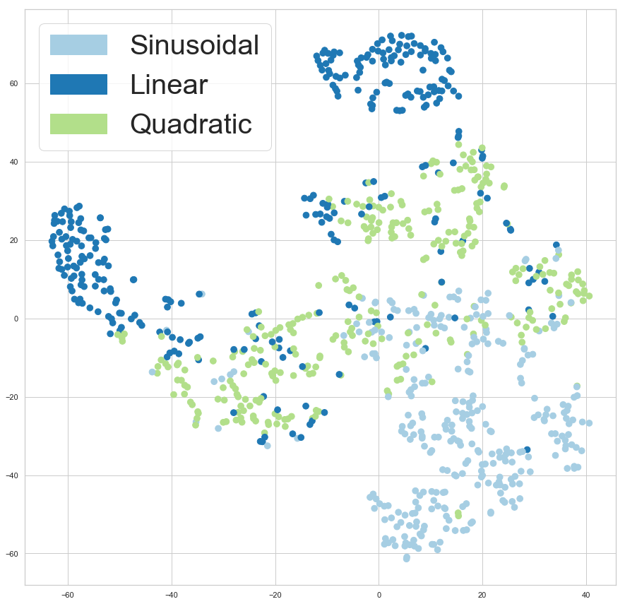
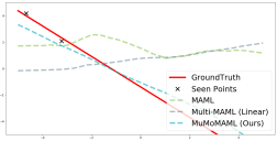
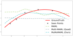
(a) MuMoMAML after modulation vs. other prior models
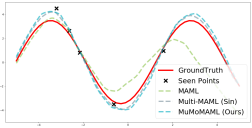
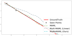
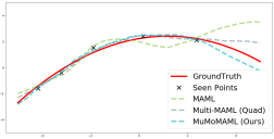
(b) MuMoMAML after adaptation vs. other posterior models			(c) Task embeddings

Figure 1: Few-shot adaptation for the multimodal regression task. (a): Without any gradient update, MuMoMAML (blue) fits target functions by modulating the meta-learned prior, outperforming the prior models of MAML (green) and Multi-MAML (gray). (b): After five steps of gradient updates, MuMoMAML outperforms MAML and Multi-MAML on all functions. More visualizations in Figure 7 and Figure 8. (c): tSNE plots of the task embeddings $\upsilon$ produced by our model from randomly sampled tasks; marker color indicates different types of functions. The plot reveals a clear clustering according to different task modes, showing that MuMoMAML is able to infer the mode from a few samples and produce a meaningful embedding. The distance among distributions aligns with the intuition of the similarity of functions (e.g. a quadratic function can sometimes be similar to a sinusoidal or a linear function while a sinusoidal function is usually different from a linear function).

We investigate our model’s capability of learning on few-shot regression tasks sampled from multimodal task distributions. In these tasks, a few input/output pairs $\{x_{k},y_{k}\}_{k=1,...,K}$ sampled from a one dimensional function are given and the model is asked to predict $L$ output values $y_{1}^{q},...,y_{L}^{q}$ for input queries $x_{1}^{q},...,x_{L}^{q}$. We set up two regression settings with two task modes (sinusoidal and linear functions) or three modes (quadratic functions added). Please see Section D for details.

As a baseline beside MAML, we propose Multi-MAML, which consists of $M$ (the number of modes) separate MAML models which are chosen for each query based on ground-truth task-mode labels. This baseline serves as an upper-bound for the performance of MAML when the task-mode labels are available. The quantitative results are shown in Table 1. We observe that Multi-MAML outperforms MAML, showing that MAML’s performance degrades on multimodal task distributions. MuMoMAML consistently achieves better results than Multi-MAML, demonstrating that our model is able to discover and exploit transferable knowledge across the modes to improve its performance. The marginal gap between the performance of our model in two and three mode settings indicates that MuMoMAML is able to clearly identify the task modes and has sufficient capacity for all modes.

We compared attention modulation with Sigmoid or Softmax and FiLM modulation and found that FiLM achieves better results. We therefore use FiLM for further experiments. Please refer to Section A for additional details. Qualitative results visualizing the predicted functions are shown in Figure 1. Figure 1 (a) shows that our model is able to identify tasks and fit to the sampled function well without performing gradient steps. Figure 1 (b) shows that our model consistently outperforms the baselines with gradient updates. Figure 1 (c) plots a tSNE maaten2008visualizing , showing the model-based module is able to identify the task modes and produce embedding vectors $\upsilon$. Additional results are shown in Section E.

3.2 Reinforcement Learning

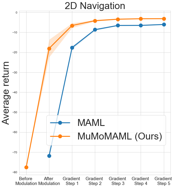
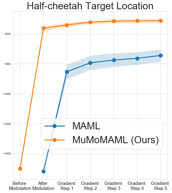
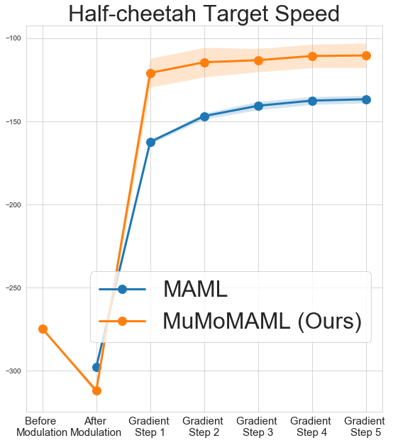
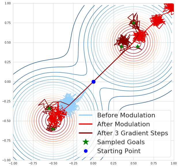
(a) 2D Navigation	(b) Target Location	(c) Target Speed	(d) 2D Navigation Results

Figure 2: (a-c) Adaptation curves for MuMoMAML and MAML baseline in 2D navigation and half-cheetah environments. The “after modulation” step represents the rewards of the modulated policy for MuMoMAML and the initial rewards for MAML. MuMoMAML outperforms MAML across the gradient update steps given a single extra trajectory. (d) Visualized trajectories sampled using MuMoMAML in the 2D navigation environment. The contours represent the probability density of the goal distribution (red: high probability; blue: low probability). The trajectories demonstrate the effect of modulation and the subsequent fine tuning with gradient steps. Additional trajectory visualizations can be found in Figure 9.

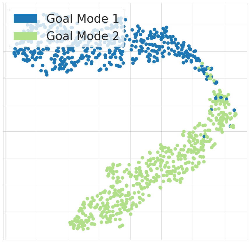
Figure 3: A tSNE plot of task embeddings of randomly sampled tasks in Target Location environment capturing the bimodal task distribution.

We experiment with MuMoMAML in three reinforcement learning (RL) environments to verify its ability to learn to rapidly adapt to tasks sampled from multimodal task distributions given a minimum amount of interaction with an environment.

2D Navigation. We utilize a 2D navigation environment with bimodal task distribution to investigate the capabilities of the embedding network to identify the task mode based on trajectories sampled from RL environments and the modulation network to modulate a policy network. In this environment, the agent is rewarded for moving close to a goal location. The model-based meta-learner is able to identify the task modes and modulate the policy accordingly, allowing efficient fast adaptation. This is shown in the agent trajectories and the average return plots presented in Figure 2 (a) and (d), where our model outperforms MAML with any number of gradient steps.

Half-cheetah Target Location and Speed. To investigate the scalability of our method to more complex RL environments we experiment with locomotion tasks based on the half-cheetah model. In the target location and target speed environments the agent is rewarded for moving close to the target location or moving at target speed respectively. The targets are sampled from bimodal distributions. In these environments, the dynamics are considerably more complex than in the 2D navigation case. MuMoMAML is able to utilize the model-based meta-learner to effectively modulate the policy network and retain an advantage over MAML across all gradient update steps as seen from the adaptation curves in Figure 2 (b) and Figure 2 (c). A tSNE plot of the embeddings in Figure 3 shows that our model is able to produce meaningful task embeddings $\upsilon$.

4 Conclusion

We presented a novel meta-learning approach that is able to leverage the strengths of both model-based and gradient-based meta-learners to discover and exploit the structure of multimodal task distributions. With the ability to effectively recognize the task modes as well as rapidly adapt through a few gradient steps, our proposed MuMoMAML achieved superior generalization performance on multimodal few-shot regression, reinforcement learning, and image classification.

Appendix A Modulation Methods

To allow efficient adaptation, the modulation network activates or deactivates units of each network block of the gradient-based meta-learner according to the given target task embedding. We investigated a representative set of modulation operations, including attention-based modulation (mnih2014recurrent, ; vaswani_attention_2017, ) and feature-wise linear modulation (FiLM) (perez_film:_2017, ).

Attention based modulation

(mnih2014recurrent, ; vaswani_attention_2017, ) has been widely used in modern deep learning models and has proved its effectiveness across various tasks (yang2016stacked, ; mnih2014recurrent, ; zhang_self-attention_2018, ; xu2015show, ). Inspired by the previous works, we employed attention to modulate the prior model. In concrete terms, attention over the outputs of all neurons (Softmax) or a binary gating value (Sigmoid) on each neuron’s output is computed by the model-based meta-learner. These parameters $\tau$ are then used to scale the pre-activation of each neural network layer $\mathbf{F}_{\theta}$, such that $\mathbf{F}_{\phi}=\mathbf{F}_{\theta}\otimes\tau$. Note that here $\otimes$ represents a channel-wise multiplication.

Feature-wise linear modulation (FiLM)

(perez_film:_2017, ) proposed to modulate neural networks to condition the networks on data from different modalities. We adopt FiLM as an option for modulating our gradient-based meta-learner. Specifically, the parameters $\tau$ are divided in to two components $\tau_{\gamma}$ and $\tau_{\beta}$ such that for a certain layer of the neural network with its pre-activation $\mathbf{F}_{\theta}$, we would have $\mathbf{F}_{\phi}=\mathbf{F}_{\theta}\otimes\tau_{\gamma}+\tau_{\beta}$. It can be viewed as a more generic form of attention mechanism. Please refer to perez_film:_2017 for the complete details.

As shown in the quantitative results (Table 1), using FiLM as a modulation method achieves better results comparing to attention mechanism with Sigmoid or Softmax. We therefore use FiLM for further experiments.

Appendix B Few-shot Image Classification

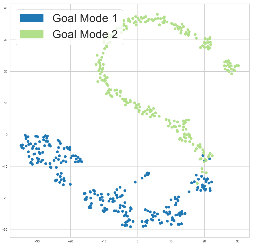
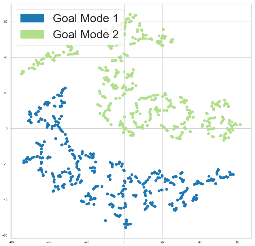
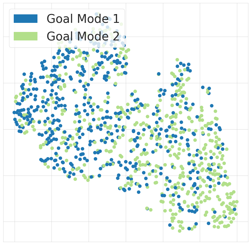
(a) Few-shot	(b) 2D Navigation	(c) 2D Navigation	(d) Target Speed
classification	interpolated goals	random goals	random goals

Figure 4: tSNE plots of task embeddings produced in different problem settings. (a) Embeddings of randomly sampled tasks in few-shot image classification. (b-c) Embeddings of tasks with goal locations interpolated between the modes and sampled randomly in 2D Navigation. (d) Randomly sampled goals in target speed environment.

The task of few-shot image classification considers a problem of classifying images into N classes with a small number (K) of labeled samples available. To evaluate our model on this task, we conduct experiments on Omniglot, a widely used handwritten character dataset of binary images. The results are shown in Table 2, demonstrating that our method achieves comparable or better results against state-of-the-art algorithms.

To gain insights to the task embeddings $\upsilon$ produced by our model, we sampled 2000 tasks randomly and employ tSNE to visualize the $\upsilon$ in Figure 4 (a). While we are not able to clearly distinguish the modes of task distributions, we observe that the distribution of the produced embeddings is not uniformly distributed or unimodal, potentially indicating the multimodal nature of this task.

Table 2: 5-way and 20-way, 1-shot and 5-shot classification accuracy on Omniglot Dataset. For each task, the best-performing method is highlighted. MuMoMAML achieves comparable or better results against state-of-the-art few-shot learning algorithms for image classification.

Method	Omniglot
	5 Way Accuracy (in %)		20 Way Accuracy (in %)
	1-shot	5-shot	1-shot	5-shot
4 Siamese nets koch2015siamese	97.3	98.4	88.2	97.0
Matching nets vinyals2016matching	98.1	98.9	93.8	98.5
Meta-SGD  li_meta-sgd:_2017	99.5	99.9	95.9	99.0
Prototypical nets snell_prototypical_2017	97.4	99.3	96.0	98.9
SNAIL mishra_simple_2017	99.1	99.8	97.6	99.4
T-net lee_gradient-based_2018	99.4	-	96.1	-
MT-net lee_gradient-based_2018	99.5	-	96.2	-
MAML (finn_model-agnostic_2017, )	98.7	99.9	95.8	98.9
MuMoMAML (ours)	99.7	99.9	97.2	99.4

Appendix C Implementation Details

For the model-based meta-learner, we used Seq2Seq (sutskever2014sequence, ) encoder structure to encode the sequence of $\{x,y\}_{k=1,...,K}$ with a bidirectional GRU (chung2014empirical, ) and use the last hidden state of the recurrent model as the representation for the task. We then apply a one-hidden-layer multi-layer perception (MLP) for each layer in the gradient-based learner’s model to generate the set of task-specific parameters $\tau_{i}$, as described in the previous section. We implemented our models for three representative learning scenarios – regression, few-shot learning and reinforcement learning. The concrete architecture for each task might be different due to each task’s data format and nature. We discuss them in the section 3.

Appendix D Additional Experimental Details

D.1 Regression

Setups.

To form multimodal task distributions, we consider a family of functions including sinusoidal functions (in forms of $A\cdot\sin{w\cdot x+b}+\epsilon$, with $A\in[0.1,5.0]$, $w\in[0.5,2.0]$ and $b\in[0,2\pi]$), linear functions (in forms of $A\cdot x+b$, with $A\in[-3,3]$ and $b\in[-3,3]$) and quadratic functions (in forms of $A\cdot(x-c)^{2}+b$, with $A\in[-0.15,-0.02]\cup[0.02,0.15]$, $c\in[-3.0,3.0]$ and $b\in[-3.0,3.0]$ ). Gaussian observation noise with $\mu=0$ and $\epsilon=0.3$ is added to each data point sampled from the target task. In all the experiments, $K$ is set to $5$ and $L$ is set to $10$. We report the mean squared error (MSE) as the evaluation criterion. Due to the multimodality and uncertainty, this setting is more challenging comparing to (finn_model-agnostic_2017, ).

Models and Optimization.

In the regression task, we trained a 4-layer fully connected neural network with the hidden dimensions of $100$ and ReLU non-linearity for each layer, as the base model for both MAML and MuMoMAML. In MuMoMAML, an additional model with a Bidirectional GRU of hidden size $40$ is trained to generate $\tau$ and to modulate each layer of the base model. We used the same hyper-parameter settings as the regression experiments presented in  finn_model-agnostic_2017 and used Adam kingma2014adam as the meta-optimizer. For all our models, we train on 5 meta-train examples and evaluate on 10 meta-val examples to compute the loss.

D.2 Reinforcement Learning

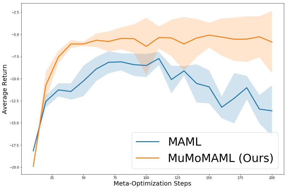
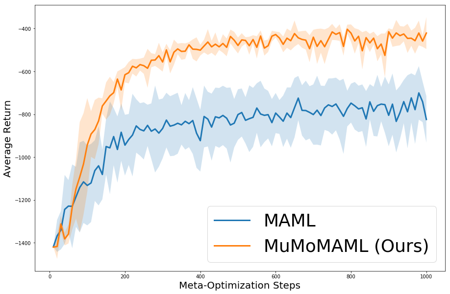
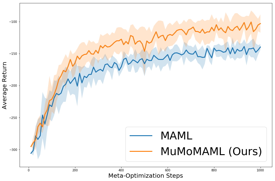
(a) 2D Navigation	(b) Target Location	(c) Target Speed

Figure 5: Training curves of MuMoMAML and MAML in reinforcement learning environments. The value indicates the performance evaluated after modulation (our model) and 5 gradient steps. The plots demonstrate that our model consistently outperforms MAML from the beginning of training to the end.

Along with few-shot classification and regression, reinforcement learning has been a central problem where meta-learning has been studied schmidhuber1997shifting ; schmidhuber1998reinforcement ; wang2016learning ; finn_model-agnostic_2017 ; mishra_simple_2017 .

To identify the mode of a task distribution in the context of reinforcement learning, we run the meta-learned prior model without modulation or adaptation to interact with the environment and collect a single trajectory and obtained rewards. Then the collected trajectory and rewards are fed to our model-based meta-learner to compute the task embedding $\upsilon$ and $\tau$. With this minimal amount of interaction with the environment, our model is able to recognize the tasks and modulate the policy network to effectively learn in multimodal task distributions.

The batch of trajectories used for computing the first gradient-based adaptation step is sampled using the modulated model and the batches after that using the modulated and adapted model from the previous update step. We follow the MAML gradient-based adaptation procedure. For the gradient adaptation steps, we use the vanilla policy gradient algorithm williams1992simple . As the meta-optimizer we use the trust region policy optimization algorithm schulman_trust_2015 .

Models and Optimization.

We use embedding model hidden size of 128 and modulation network hidden size of 32 for all environments. The training curves for all environments are presented in Figure 5, which show that our proposed model consistently outperforms MAML from the beginning of training to the end. During optimization we save model parameters and evaluate the model with five gradient update steps every 10 meta update steps. We compute the adaptation curves presented in Figure 2 using the model which achieved the best score after the five gradient updates during training.

2D-Navigation

In the 2D navigation environment the goals are sampled with equal probability from one of two bivariate Gaussians with means of $(0.5,0.5)$ and $(-0.5,-0.5)$ and standard deviation of $0.1$. In the beginning of each episode, the agent starts at the origin. The agent’s observation is its 2D-location and the reward is the negative distance to the goal. The agent does not observe the goal directly, instead it must learn to navigate there based on the reward function alone. The agent outputs vectors which elements are clipped to the range $[-0.1,0.1]$ and the agent is moved in the environment by the clipped vector. The episode terminates after 100 steps or when the agent comes to the distance of $0.01$ from the goal.

For both MuMoMAML and MAML we sample 20 trajectories for computing the gradient-based adaptation steps and 20 tasks for meta update steps. We use inner loop update step size of $0.1$ for MAML and $0.05$ for MuMoMAML. We train both methods for 200 meta-optimization steps.

We investigate the behavior of the task embedding network by sampling tasks from the environment and computing a tSNE plot of the task embeddings. A tSNE plot for goals interpolated between the goal modes is presented in Figure 4 (b) and a plot for randomly sampled goals is presented in (c). The tSNE plots show that the structure of the embedding space reflects the goal distribution.

Target Location

Target location is a locomotion environment based on the half-cheetah model in the mujoco todorov2012mujoco simulation framework. The environment design follows finn_model-agnostic_2017 , except for the reward definition. The reward on each time step is

$$R(s)=-1*abs(x_{torso}-x_{goal})+\lambda_{control}*\|a\|^{2}$$

where $x_{torso}$ and $x_{goal}$ are the x-positions of the midpoint of the half-cheetah’s torso and the target location respectively, $\lambda_{control}=-0.05$ is the coefficient for the control penalty and $a$ is the action chosen by the agent. The target location is sampled from a distribution consisting of two Gaussians with means of $-7$ and $7$ and standard deviation of $2$. The observation is the location and movement state of the joints of the half-cheetah. The episode terminates after 200 steps.

For both MuMoMAML and MAML we sample 20 trajectories for computing the gradient-based adaptation steps and 40 tasks for meta update steps. We use inner loop update step size of $0.05$ for both methods. Both methods are trained for 1000 meta-optimization steps.

Target Speed

Target speed is another half-cheetah based locomotion environment. The environment design is similar to the target location environment, except the reward is based on achieving target speed. The reward on each time step is

$$R(s)=-1*abs(v_{agent}-v_{target})+\lambda_{control}*\|a\|^{2}$$

where $v_{agent}$ and $v_{target}$ are the speed of the head of the half-cheetah and the target speed respectively, $\lambda_{control}=-0.05$ is the coefficient for the control penalty and $a$ is the action chosen by the agent. The target speed is sampled from a distribution consisting of two Gaussians with means of $-1$ and $1.5$ and standard deviation of $0.5$. The observation and other environment details are the same as in the target location environment. For training MuMoMAML and MAML same hyperparameters are used in as for target location environment.

A tSNE plot of randomly sampled task embeddings from the target speed environment is presented in Figure 4 (d). The embeddings for tasks from different modes are distributed towards the opposite ends of the tSNE plot, but the modes are not as clearly distinguishable as in the other environments. Also, the modulated policy in the target speed environment achieves lower returns than in other environments as is evident from Figure 2. Notice that in the reinforcement learning setting, the model is not optimized to achieve high returns immediately after the modulation step but only after modulation and one gradient update. After one gradient step MuMoMAML consistently outperforms MAML in target speed as well.

D.3 Few-shot Image Classification

Setups.

In the few-shot learning experiments, we used Omniglot, a dataset consists of 50 languages, with a total of 1632 different classes with 20 instances per class. Following santoro_meta-learning_2016 , we downsampled the images to $28\times 28$ and perform data augmentation by rotating each member of an existing class by a multiple of 90 degrees to form new data points.

Models and Optimization.

Following prior works (vinyals2016matching, ; finn_model-agnostic_2017, ), we used the same 4-layer convolutional neural network and applied the same training and testing splits from finn_model-agnostic_2017 and compare our model against baselines for 5-way and 20-way, 1-shot and 5-shot classification.

Appendix E Additional Experimental Results

E.1 Additional Results for Regression

Figure 6 demonstrates that MuMoMAML outperforms the MAML and Multi-MAML baselines no matter how many gradient steps are performed. Also, MuMoMAML is able to achieve good performance solely based on modulation without any gradient update, showing that our model-based meta-learner is capable of identifying the mode of a multimodal task distribution and effectively modulate the meta-learned prior.

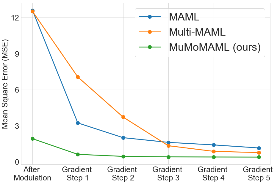
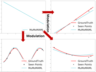
(a) Performance upon updates	(b) Effect of modulation

Figure 6: (a) Comparing the models’ performance with respect to the number of gradient updates applied. For MuMoMAML, we report the performance after modulation for gradient step 0. (b) A demonstration of the modulation on prior model by our model-based meta-learner. With the FiLM modulation, MuMoMAML can adapt to different priors before gradient-based adaptation.

Additional qualitative results for MuMoMAML after modulation are shown in Figure 7 and additional qualitative results for MuMoMAML after adaptation are shown in Figure 8.

E.2 Additional Qualitative Results for Reinforcement Learning

Additional trajectories sampled from the 2D navigation environment are presented in Figure 9.

Sinusoidal Functions	Linear Functions	Quadratic Functions

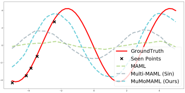
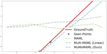
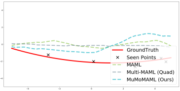
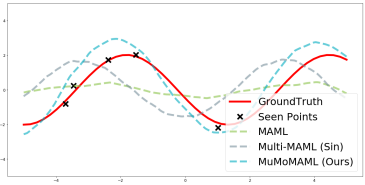
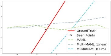
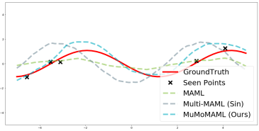
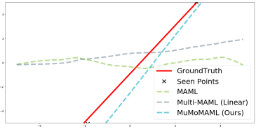
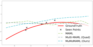
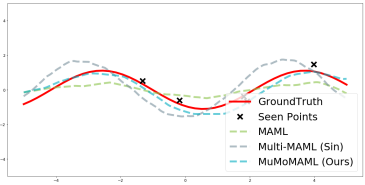
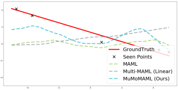
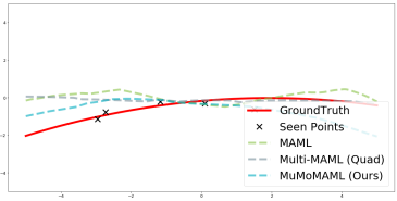
Figure 7: Additional qualitative results of the regression tasks. MuMoMAML after modulation vs. other prior models.

Sinusoidal Functions	Linear Functions	Quadratic Functions

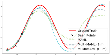
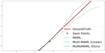
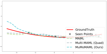
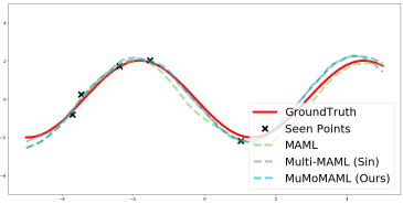
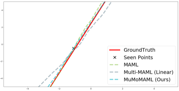
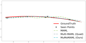
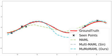
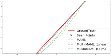
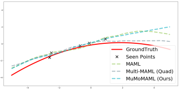
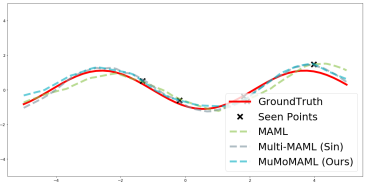
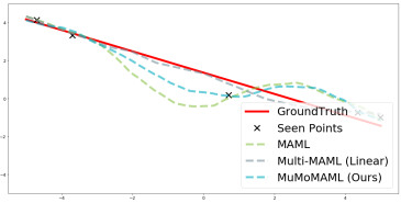
Figure 8: Additional qualitative results of the regression tasks. MuMoMAML after adaptation vs. other posterior models.

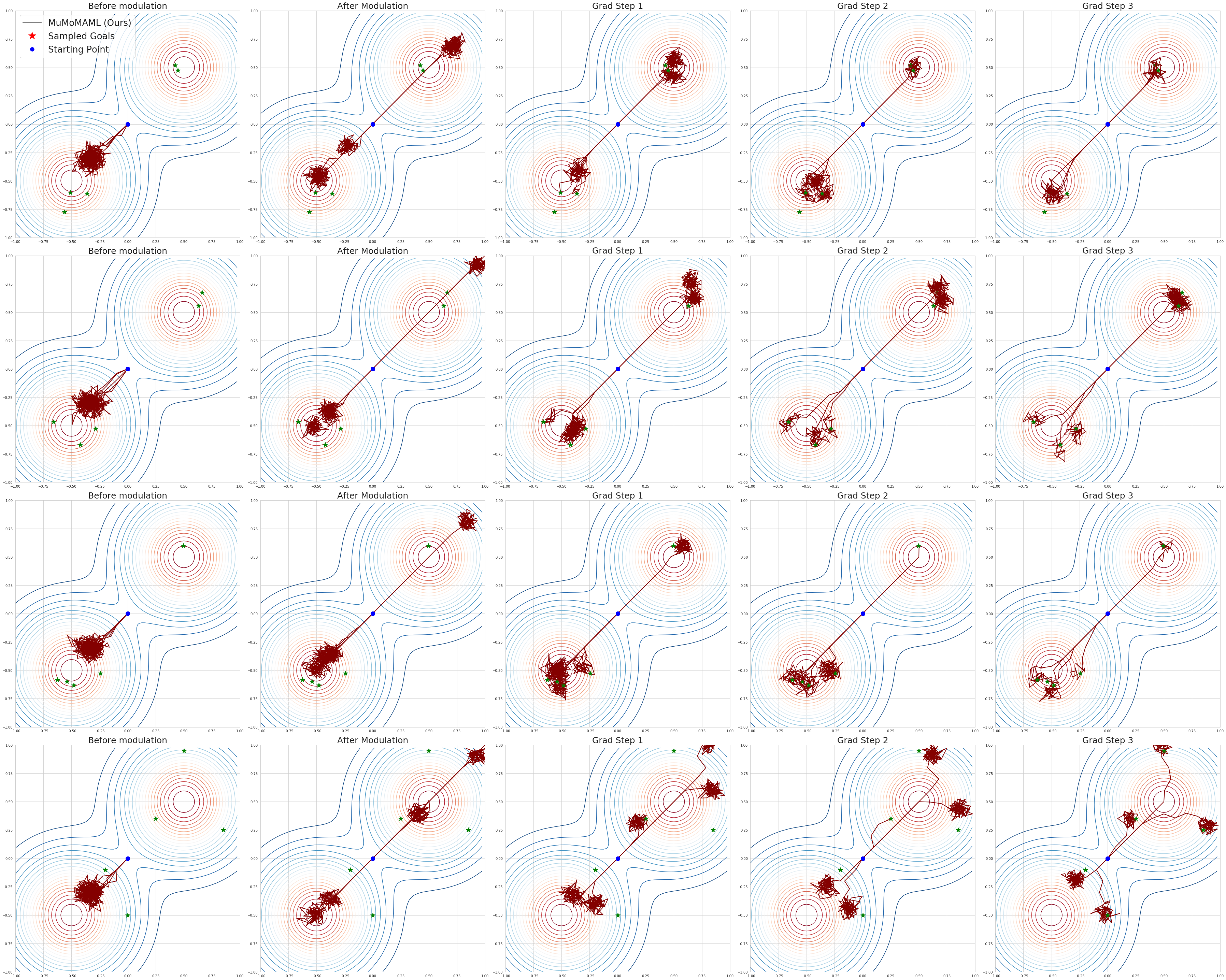
Figure 9: Additional trajectories sampled from the 2D navigation environment with MuMoMAML. The first four rows are with goals sampled from the environment distribution, where MuMoMAML demonstrates rapid adaptation and is often able to locate the goal exactly. On the fifth row, trajectories are sampled with less probable goals. The agent is left farther away from the goals after the modulation step, but the gradient based adaptation steps then steadily recover the performance.

References

- (1) Marcin Andrychowicz, Misha Denil, Sergio Gomez Colmenarejo, Matthew W. Hoffman, David Pfau, Tom Schaul, and Nando de Freitas. Learning to learn by gradient descent by gradient descent. In Advances in Neural Information Processing Systems, 2016.
- (2) Samy Bengio, Yoshua Bengio, Jocelyn Cloutier, and Jan Gecsei. On the optimization of a synaptic learning rule. In Preprints Conf. Optimality in Artificial and Biological Neural Networks, 1992.
- (3) Junyoung Chung, Caglar Gulcehre, KyungHyun Cho, and Yoshua Bengio. Empirical evaluation of gated recurrent neural networks on sequence modeling. arXiv preprint arXiv:1412.3555, 2014.
- (4) Yan Duan, John Schulman, Xi Chen, Peter L Bartlett, Ilya Sutskever, and Pieter Abbeel. Rl 2: Fast reinforcement learning via slow reinforcement learning. arXiv preprint arXiv:1611.02779, 2016.
- (5) Chelsea Finn, Pieter Abbeel, and Sergey Levine. Model-agnostic meta-learning for fast adaptation of deep networks. In International Conference on Machine Learning, 2017.
- (6) Chelsea Finn, Kelvin Xu, and Sergey Levine. Probabilistic Model-Agnostic Meta-Learning. In Advances in Neural Information Processing Systems, 2018.
- (7) Erin Grant, Chelsea Finn, Sergey Levine, Trevor Darrell, and Thomas Griffiths. Recasting Gradient-Based Meta-Learning as Hierarchical Bayes. In International Conference on Learning Representations, 2018.
- (8) Sepp Hochreiter, A Steven Younger, and Peter R Conwell. Learning to learn using gradient descent. In International Conference on Artificial Neural Networks, pages 87–94. Springer, 2001.
- (9) Taesup Kim, Jaesik Yoon, Ousmane Dia, Sungwoong Kim, Yoshua Bengio, and Sungjin Ahn. Bayesian Model-Agnostic Meta-Learning. In Neural Information Processing Systems, 2018.
- (10) Diederik P Kingma and Jimmy Ba. Adam: A method for stochastic optimization. In International Conference on Learning Representations, 2015.
- (11) Gregory Koch, Richard Zemel, and Ruslan Salakhutdinov. Siamese neural networks for one-shot image recognition. In Deep Learning Workshop at International Conference on Machine Learning, 2015.
- (12) Yoonho Lee and Seungjin Choi. Gradient-Based Meta-Learning with Learned Layerwise Metric and Subspace. In International Conference on Machine Learning, 2018.
- (13) Zhenguo Li, Fengwei Zhou, Fei Chen, and Hang Li. Meta-SGD: Learning to Learn Quickly for Few-Shot Learning. arXiv preprint arXiv:1707.09835, 2017.
- (14) Laurens van der Maaten and Geoffrey Hinton. Visualizing data using t-sne. Journal of Machine Learning Research, 2008.
- (15) Nikhil Mishra, Mostafa Rohaninejad, Xi Chen, and Pieter Abbeel. A Simple Neural Attentive Meta-Learner. In International Conference on Learning Representations, 2018.
- (16) Volodymyr Mnih, Nicolas Heess, Alex Graves, et al. Recurrent models of visual attention. In Advances in Neural Information Processing Systems, 2014.
- (17) Tsendsuren Munkhdalai and Hong Yu. Meta networks. In International Conference on Machine Learning, 2017.
- (18) Ethan Perez, Florian Strub, Harm de Vries, Vincent Dumoulin, and Aaron C. Courville. Film: Visual reasoning with a general conditioning layer. In Association for the Advancement of Artificial Intelligence, 2018.
- (19) Sachin Ravi and Hugo Larochelle. Optimization as a Model for Few-Shot Learning. In International Conference on Learning Representations, 2017.
- (20) Adam Santoro, Sergey Bartunov, Matthew Botvinick, Daan Wierstra, and Timothy Lillicrap. Meta-Learning with Memory-Augmented Neural Networks. In International Conference on Machine Learning, 2016.
- (21) Jurgen Schmidhuber. Evolutionary principles in self-referential learning. on learning now to learn: The meta-meta-meta…-hook. Master’s thesis, Technische Universitat Munchen, Germany, 1987.
- (22) Jürgen Schmidhuber, Jieyu Zhao, and Nicol N Schraudolph. Reinforcement learning with self-modifying policies. In Learning to learn, pages 293–309. Springer, 1998.
- (23) Jürgen Schmidhuber, Jieyu Zhao, and Marco Wiering. Shifting inductive bias with success-story algorithm, adaptive levin search, and incremental self-improvement. Machine Learning, 1997.
- (24) John Schulman, Sergey Levine, Philipp Moritz, Michael I. Jordan, and Pieter Abbeel. Trust Region Policy Optimization. In International Conference on Machine Learning, 2015.
- (25) Pranav Shyam, Shubham Gupta, and Ambedkar Dukkipati. Attentive recurrent comparators. arXiv preprint arXiv:1703.00767, 2017.
- (26) Jake Snell, Kevin Swersky, and Richard S. Zemel. Prototypical Networks for Few-shot Learning. In Advances in Neural Information Processing Systems, 2017.
- (27) Flood Sung, Yongxin Yang, Li Zhang, Tao Xiang, Philip H.S. Torr, and Timothy M. Hospedales. Learning to compare: Relation network for few-shot learning. In IEEE Conference on Computer Vision and Pattern Recognition, 2018.
- (28) Ilya Sutskever, Oriol Vinyals, and Quoc V Le. Sequence to sequence learning with neural networks. In Advances in Neural Information Processing Systems, 2014.
- (29) Emanuel Todorov, Tom Erez, and Yuval Tassa. Mujoco: A physics engine for model-based control. In International Conference On Intelligent Robots and Systems, 2012.
- (30) Ashish Vaswani, Noam Shazeer, Niki Parmar, Jakob Uszkoreit, Llion Jones, Aidan N. Gomez, Lukasz Kaiser, and Illia Polosukhin. Attention Is All You Need. In Advances in Neural Information Processing Systems, 2017.
- (31) Oriol Vinyals, Charles Blundell, Tim Lillicrap, Daan Wierstra, et al. Matching networks for one shot learning. In Advances in Neural Information Processing Systems, 2016.
- (32) Jane X Wang, Zeb Kurth-Nelson, Dhruva Tirumala, Hubert Soyer, Joel Z Leibo, Remi Munos, Charles Blundell, Dharshan Kumaran, and Matt Botvinick. Learning to reinforcement learn. arXiv preprint arXiv:1611.05763, 2016.
- (33) Ronald J Williams. Simple statistical gradient-following algorithms for connectionist reinforcement learning. Machine learning, 1992.
- (34) Kelvin Xu, Jimmy Ba, Ryan Kiros, Kyunghyun Cho, Aaron Courville, Ruslan Salakhudinov, Rich Zemel, and Yoshua Bengio. Show, attend and tell: Neural image caption generation with visual attention. In International Conference on Machine Learning, 2015.
- (35) Zichao Yang, Xiaodong He, Jianfeng Gao, Li Deng, and Alex Smola. Stacked attention networks for image question answering. In IEEE Conference on Computer Vision and Pattern Recognition, 2016.
- (36) Han Zhang, Ian Goodfellow, Dimitris Metaxas, and Augustus Odena. Self-Attention Generative Adversarial Networks. axXiv preprint arXiv:1805.08318, 2018.