Passivity Analysis of Replicator Dynamics and its Variations

Abstract

In this paper, we focus on studying the passivity properties of different versions of replicator dynamics (RD). RD is an important class of evolutionary dynamics in evolutionary game theory. Evolutionary dynamics describe how the population composition changes in response to the fitness levels, resulting in a closed-loop feedback system. RD is a deterministic monotone non-linear dynamic that allows incorporation of the distribution of population types through a fitness function. Here, in this paper, we use a tools for control theory, in particular, the passivity theory, to study the stability of the RD when it is in action with evolutionary games. The passivity theory allows us to identify class of evolutionary games in which stability with RD is guaranteed. We show that several variations of the first order RD satisfy the standard loseless passivity property. In contrary, the second order RD do not satisfy the standard passivity property, however, it satisfies a similar dissipativity property known as negative imaginary property. The negative imaginary property of the second order RD allows us to identify the class of games that converge to a stable equilibrium with the second order RD.

I Introduction

Population games [1, 2] is a class of games that model interactions between a large number of agents (named players in game theory contest), in which each player or agent’s payoff depends on his own strategy and the distribution of strategies of other agents. There has been extensive research in a variety of settings, ranging from societal [3] to biological [4] to engineered [5].

In population games, and learning in games [6, 7, 8], one of the main points is to understand the behavior of the agent strategies on the long run. In particular, understanding the convergence and divergence of population strategies to a particular solution concept such as Nash equilibrium. The convergence or divergence of such strategies will depend on both the game under consideration as well as the evolutionary dynamics [9, 10]. Some specific games can exhibit inherent obstacles to convergence for a cluster of evolutionary dynamics [11].

Replicator dynamics (RD) is one of the most studied game dynamics in the literature of evolutionary game theory. RD was introduced as a non-linear first-order differential equations in [12] to model a single species and given the name of RD in [13]. The RD has been used extensively in modeling game dynamics including biological systems in order to predict the evolutionary behavior without a detailed analysis of such biological factors as genetic or population size effects [14].

Passivity theory is a very well established sub-class of control theory, which implies useful properties such as stability, and the importance of passivity as tool in nonlinear control of interconnected systems—unlike Lyapunov stability criteria—relays on the fact that any set of passive sub-systems in parallel or feedback configuration forms a passive system. Passivity is an input-output property of a class of nonlinear physical systems which can only consume energy. The notion of passivity originally comes from electric circuits composed of resistors, capacitors, and inductors. The same definition applies to analogous mechanical and hydraulic systems. This idea can be extended to study electric circuits with nonlinear passive components and magnetic couplings. For a detailed discussion on passive systems see [2, 3, 4, 5] and the references therein, which show that passive systems theory received a great deal of attention in the last few decades. When a passive system is connected to a strictly passive system in a negative feedback loop, energy is strictly dissipated as signals propagate around the loop, and hence the feedback interconnection is stable. In other words, by ensuring that every subsystem is passive, a complex structure of subsystems can be built to satisfy certain properties.

In [15], the relationship between passivity theory and class of population games and dynamics was established. It was shown that what is called contractive games can be considered as passive games where it satisfies similar properties to passive systems. Similarly, many evolutionary dynamics also satisfy the passivity property. This implies that the feedback interconnections of passive evolutionary dynamics with passive game exhibit stable behavior. The above connection between passivity theory and population games and dynamics enables the opportunity to analyze in a similar way similar classes of games and evolutionary dynamics, for instance, higher order games and higher order dynamics.

In the standard population games, the fitness function of the population strategies is a static function of the population composition. However, in higher order population games, dependence can be dynamic, e.g., as a model of path dependencies [15]. Similarly, in the standard form evolutionary dynamics, the number of states is equal to the number of population strategies. However, higher order dynamics is able to introduce different behaviors [11, 16, 17, 18]. Also, in [19], the higher order version of the replicator dynamics can eliminate weakly dominated strategies, which is not the case in the canonical replicator dynamics.

In this paper, we focus on studying the passivity property of several variations of the well know replicator dynamics, including the higher order replicator dynamics. We show that the standard replicator dynamics satisfy the lossles passivity property. Also, the local version of replicator dynamics satisfy the lossles property. However, the higher order of the replicator dynamics do not satisfy the passivity property. Instead, it satisfy the negative imaginary property, which can be considered as a counterpart of the passivity theory. The Negative imaginary theory also have a similar stability conditions to those in passivity theory.

The remainder of this paper is organized as follows: Section II presents preliminary material on population games, passivity and negative imaginary systems. Section III presents the concept of higher order games and dynamics. Section IV presents the passivity property for different variations of the replicator dynamics. Section V inderduces the notion of passiviation for replicator dynamics. Finally, Section VI contains concluding remarks.

II Preliminaries and notations

This section presents the required preliminaries and notations from input-output operators, game theory, replicator dynamics and passivity theory.

II-A Input-output operators

Dynamical system can be seen as an operator defined on function spaces. Suppose that $\mathbb{L}_{2}$ denote the Hilbert space of square integrable functions, which maps $\mathbb{R}_{+}$ to $\mathbb{R}^{n}$ with inner product $\langle\cdot,\cdot\rangle$ and $\lVert\cdot\lVert$. Let $\mathbb{L}_{2e}$ denote the space of functions that are square integrable over finite intervals.

$$\mathbb{L}_{2e}=\left\{f:\mathbb{R}_{+}\rightarrow\mathbb{R}_{n}:\int_{0}^{\infty}f(t)^{T}f(t)dt\leq\infty\;\forall\;T\in\mathbb{R}\right\}.$$ (1)

For $\mathbb{U}$,$\mathbb{Y}$ $\subset$ $\mathbb{L}_{2e}$ subsets of functions, an input-output operator is a mapping $S:\mathbb{U}\rightarrow\mathbb{Y}$.

II-B Passivity theory

Passivity theory is a useful tool to assess the stability of a feedback interconnection. In brief, if both components of a feedback interconnection have the passivity property, then the closed loop interconnection is stable [20, 21, 15]. A game theoretic context to passivity in games including the definition of passive games was given in [15].

Define $\Sigma$ to be a nonlinear dynamical system with the following state space description:

$$\dot{x} =f(x,u),\;\;\;\;\;\;x(0)=x_{0},$$ (2)

$$y =g(x,u),$$

where, $u(t)\in\mathbf{U}\subset\mathbb{R}^{m}$ is the system’s input vector, $x_{0}\in\mathbf{M}\subset\mathbb{R}^{n}$, $y\in\mathbb{R}^{m}$ is the system’s output vector and $x(t)\in\mathbb{R}^{n}$ is the system’s state vector. Also, assume that for some classes of functions, $\mathbb{U}$ and $\mathbb{Y}$, and for any initial condition in $\mathbf{M}$, there exists a solution for all $u\in\mathbb{U}$ resulting in $y\in\mathbb{Y}$ and $x(t)\in\mathbf{M}$ all $t\geq 0$. Next, we present two definitions for passive system from both state space and input-output perspectives.

Definition 1

The nonlinear system $\Sigma$ with state space (2) is said to be passive if there exists a storage function $L:\mathbf{M}\rightarrow\mathbb{R_{+}}$ such that for all $x_{0}\in\mathbf{M}$ and $t\geq 0$,

$$L(x(t))\leq L(x_{0})+\int_{0}^{t}\!u(\tau)^{T}y(\tau)d\tau.$$ (3)

The input-output definition of passivity property is given as follows:

Definition 2

The input-output operator $S:\mathbb{U}\rightarrow\mathbb{Y}$ is said to be passive if there exist constant $\alpha$ such that:

$$\langle Su,u\rangle_{T}\geq\alpha,\forall\;u\in\mathbb{U},T\in\mathbb{R}_{+},$$ (4)

and input strictly passive if there exist $\beta>0$ and $\alpha$ such that

$$\langle Su,u\rangle_{T}\geq\alpha,+\beta\langle u,u\rangle_{T}\forall\;u\in\mathbb{U},T\in\mathbb{R}_{+},$$ (5)

where, $\langle f,g\rangle_{T}=\int_{0}^{T}f(t)^{T}g(t)dt$.

In the case of equality in the inequalities (3) and (4), the system is said to be lossless.

The stability of the feedback interconnection between passive systems is a fundamental result in passivity theory (e.g., [22]). That is, the negative feedback interconnection between a passive system $\Sigma_{1}$ and strictly passive $\Sigma_{2}$, as shown in Fig. 1, is stable feedback interconnection. Also, the closed loop system from $r$ to $y_{1}$ is passive.

Figure 1: Negative feedback interconnection.

II-C Negative imaginary systems theory

Negative imaginary (NI) systems theory was introduced by Lanzon and Petersen in [23, 24] for linear time invariant systems to control systems with flexible structure dynamics. Several generalization for the the negative imaginary theory can be found in [25, 26, 27]. NI systems theory complements the limitations of passivity theory in linear systems, which is only applicable for systems with relative degree zero or one. Recently, nonlinear version of negative imaginary system theory was developed in [28]. In this section, we recall the definition of NI and SNI systems as given in [29]. We also define some notations that will be used in the paper.

Consider the following LTI system,

$$\dot{x}(t)=Ax(t)+Bu(t),$$ (6)

$$y(t)=Cx(t)+Du(t),$$ (7)

where $A\in\mathbb{R}^{n\times n},B\in\mathbb{R}^{n\times m},C\in\mathbb{R}^{m\times n},$ $D\in\mathbb{R}^{m\times m},$ and with the square transfer function matrix $G(s)=C(sI-A)^{-1}B+D$. The transfer function matrix $G(s)$ is said to be strictly proper if $G(\infty)=D=0$. We will use the notation $\begin{bmatrix}\begin{array}[]{c|c}A&B\\ \hline\cr C&D\end{array}\end{bmatrix}$ to denote the state space realization (6), (7).

The NI system is defined as follows;

Definition 3

[30, 29] A square transfer function matrix $G(s)$ is NI if the following conditions are satisfied:

1. $G(s)$ has no pole in $Re[s]>0$.

2. For all $\omega>0$ such that $s=j\omega$ is not a pole of $G(s)$,

   $$j\left(G(j\omega)-G(j\omega)^{\ast}\right)\geq 0.$$ (8)

3. If $s=j\omega_{0}$ with $\omega_{0}>0$ is a pole of $G(s)$, then it is a simple pole and the residue matrix $K=\underset{s\longrightarrow j\omega_{0}}{\lim}(s-j\omega_{0})jG(s)$ is Hermitian and positive semidefinite.

4. If $s=0$ is a pole of $G(s)$, then $\underset{s\longrightarrow 0}{\lim}s^{k}G(s)=0$ for all $k\geq 3$ and $\underset{s\longrightarrow 0}{\lim}s^{2}G(s)$ is Hermitian and positive semidefinite.

Definition 4

[25] A square transfer function matrix $G(s)$ is SNI if the following conditions are satisfied:

1. ${G}(s)$ has no pole in $Re[s]\geq 0$.

2. For all $\omega>0$, $j\left({G}(j\omega)-{G}(j\omega)^{\ast}\right)>0$.

Here, we present an NI lemma.

Lemma 1

Let $\begin{bmatrix}\begin{array}[]{c|c}A&B\\ \hline\cr C&D\end{array}\end{bmatrix}$ defining the system (6)-(7) be a minimal realization of the transfer function matrix $G(s)$. Then, $G(s)$ is NI if and only if $D=D^{T}$ and there exist matrices $P=P^{T}\geq 0$, $W\in\mathbb{R}^{m\times m}$, and $L\in\mathbb{R}^{m\times n}$ such that the following linear matrix inequality (LMI) is satisfied:

$$\begin{bmatrix}PA+A^{T}P&PB-A^{T}C^{T}\\ B^{T}P-CA&-(CB+B^{T}C^{T})\end{bmatrix}=\begin{bmatrix}-L^{T}L&-L^{T}W\\ -W^{T}L&-W^{T}W\end{bmatrix}\leq 0.$$ (9)

The positive feedback interconnection between an NI system with transfer function matrix $G(s)$ and an SNI system with transfer function matrix $\bar{G}(s)$ as shown in Fig. 2. Also, suppose that the transfer function matrix $G(s)$ has a minimal state space realization $\begin{bmatrix}\begin{array}[]{c|c}A&B\\ \hline\cr C&D\end{array}\end{bmatrix},$ and $\bar{G}(s)$ has a minimal state space realization $\begin{bmatrix}\begin{array}[]{c|c}\bar{A}&\bar{B}\\ \hline\cr\bar{C}&\bar{D}\end{array}\end{bmatrix}.$ Furthermore, it is assumed that the matrix $I-D\bar{D}$ is nonsingular. Then the closed system has a system matrix given by

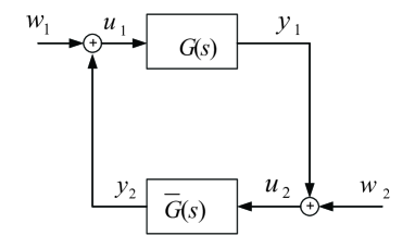
Figure 2: A negative-imaginary feedback control system. If the plant transfer function matrix $G(s)$ is NI and the controller transfer function matrix $\bar{G}(s)$ is SNI, then the positive-feedback interconnection is internally stable if and only if the DC gain condition, $\lambda_{max}(G(0)\bar{G}(0))<1,$ is satisfied.

$$\breve{A}=\begin{bmatrix}A+B\bar{D}(I-D\bar{D})^{-1}C&B\bar{C}+B\bar{D}(I-D\bar{D})^{-1}D\bar{C}\\ \bar{B}(I-D\bar{D})^{-1}C&\bar{A}+\bar{B}(I-D\bar{D})^{-1}D\bar{C}\end{bmatrix}.$$ (10)

Moreover, the positive feedback interconnection between $G(s)$ and $\bar{G}(s)$ as shown in Fig. 2 and denoted $[G(s),\bar{G}(s)]$ is said to be internally stable if the closed-loop system matrix $\breve{A}$ in (10) is Hurwitz; e.g., see [31].

A nonlinear definition of NI system is given as follows: Consider the following general nonlinear system

$$\dot{x} =f(x,u)$$ (11)

$$y =h(x)$$ (12)

where $f:\mathbb{R}^{n}\times\mathbb{R}\rightarrow\mathbb{R}^{n}$ is Lipschitz continuous function and $h:\mathbb{R}^{n}\rightarrow\mathbb{R}$ is a class $C^{1}$ function.

Definition 5

The nonlinear system (11), (12) is Negative Imaginary if there exists a positive storage function $V:\mathbb{R}^{n}\rightarrow\mathbb{R}$ of a class $C^{1}$ such that

$$\dot{V}(x(t))\leq\dot{y}(t)u(t).$$ (13)

Definition 6

The nonlinear system (11), (12) is Negative Imaginary if there exists a positive storage function $V:\mathbb{R}^{n}\rightarrow\mathbb{R}$ of a class $C^{1}$ such that

$$V(x(t))\leq V(x(0))+\int_{0}^{t}y(s)^{T}\int_{0}^{s}u(\tau)d\tau ds,$$ (14)

for all $t>0$.

Or,

$$\dot{V}(x(t))\leq y(t)^{T}\int_{0}^{t}u(\tau)d\tau.$$ (15)

The main difference between the NI definition given in (5) and passivity definition is the use of $\dot{y}(t)$ instead of ${y}(t)$ in calculating the supplied energy rate.

II-D Population games

A game, in general, consist of three basic elements. Number of players $N$: are the decision makers in the game context. Strategies $S$: are the set of actions that a particular player will play given a set of conditions and circumstances that will emerge in the game being played. Payoff $P$: is the reward which a player receives from playing at a particular strategy. In general, game is viewed as a mapping from strategies $x\in X$, where $X=\{x:\;\;\Sigma_{i\in S}x_{i}=1\}$, to Payoff $F(x)$. This viewpoint can be extended in dynamic setting to a mapping of strategy trajectories $x(\cdot)$ to payoff trajectories $F(\cdot)$. In other words, games can be described as a dynamical systems with states, inputs and outputs.

A single population game has a set of strategies $S=\{1,2,...,m\}$ and a set of strategy distributions $X=\{x:\;\;\Sigma_{i\in S}x_{i}=1\}$. Since strategies lie in the simplex, admissible changes in strategy are restricted to the tangent space $TX=\{z\in\mathbb{R}^{m}:\sum_{i\in s}z_{i}=0\}$.

Now, define $F(x):S\longrightarrow\mathbb{R}^{m}$ to be the payoff function that associate each strategy distribution in $S$ with a payoff vector so that $F_{i}:S\longrightarrow\mathbb{R}^{m}$ is the payoff to strategy $i\in S$. Also, define $DF(x)$ to be the Jacobian matrix of $F(x)$. A state $x^{*}\in X$ is a Nash equilibrium if each strategy in the support of $x$ receives the maximum payoff available to the population.

II-E Evolutionary dynamics

In general game theory setup, the prediction of the game outcome and its equilibrium analysis depends on what game players know about it. In such setup, a assumption such as full rationality of players is always made.

A slightly different approach to study the game behavior, in particular for games that have repetitive interactions among a large number of players, is disequilibrium analysis. Here, players meant to adjust and revise the chose of their strategies based on the their current strategies as well as the state of the collective population when a feedback is given. In this setup, the revision protocol, is used to organize the procedure of how and when agents change their strategies.

Figure 3: Feedback interconnection of a dynamic and a game, where $P$ is the payoffs and $X$ is the strategies.

Revision protocol can be considered as a mapping from payoffs to strategy distributions under a particular conditional switch rate $\rho_{ij}$. A population game $F$ with a revision protocol $\rho_{ij}$ creates the mean dynamic, which is given as follows:

$$\dot{x_{i}}=\sum_{j\in S}x_{j}\rho_{ij}-x_{i}\sum_{j\in S}\rho_{ij}.$$ (16)

Throughout the mean dynamic given in (16) and different revision protocols $\rho_{ij}$, one can create different evolutionary dynamics that maps payoffs to new strategy distribution. Then, this new strategy distribution is mapped by the game to generate new vector of payoffs as shown in Fig. 3. This analogy is similar to the feedback interconnections in control systems setups.

For instance, the replicator dynamic is generated using the imitation of success revision protocol, which is given as follows:

$$\rho_{ij}=x_{j}(p_{j}-K),$$ (17)

where $K$ is a constant less than or equal to any $p_{j}$. By substituting (17) into the mean dynamic (16), we get the replicator dynamics equations as follows:

$$\dot{x_{i}}=x_{i}(p_{i}-\sum_{j}x_{j}p_{j}),$$ (18)

where $p_{i}$ is the payoff for using strategy $i$.

Another representation of the replicator dynamics Equation (18) is cascaded connection between an integrator and Gibbs distribution as shown in Fig. 4.

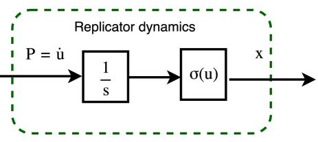
Figure 4: Replicator dynamics (18) as a cascaded connection between integrator and Gibbs distribution.

.

III Higher-order dynamics and games

As we indicated in the previous section, the standard game is a static mapping from strategies $X$ to a set of real valued payoffs $P$,

$$P=F(x),$$

and the evolutionary dynamic is restricted first order mapping from payoffs $P$ to strategies $X$,

$$\dot{x}=V(x,p).$$

The dynamical view of this feedback loop can be extended to a mapping of strategy trajectories to payoff trajectories. This viewpoint allows the introduction of generalized forms of dynamics and games, such as higher-order dynamics and games, to generate these trajectories.

Higher-order dynamics can be introduced—independent of the game—through auxiliary states to the the first order dynamics [17, 18], which can be interpreted as path dependency. Also, similar higher-dynamics can be obtained by the direct derivative of the first order dynamics [19]. It has been shown in [11, 16, 17, 18, 19] that modification of the standard dynamics can exhibit qualitatively different behaviors. One form of generalized higher-order dynamics obtained by inducing an auxiliary state $z$ int the dynamics. In this case, a higher-order dynamics takes the following form:

$$\dot{z} =f(z,p)\;\;\;\;\;z(0)=z_{0},$$

$$x =g(z,p),$$

where, for all $x(0)$ in the simplex and for all bounded $p(\cdot)$, there exists $x^{*}$ and $p^{*}$ such that if $p(t)\rightarrow p^{*}$, then, $x(t)\rightarrow x^{*}$.

Furthermore, higher-order dynamics can be introduced by processing the payoff. Here, the processing might include an integral action, which means taking the payoff history into the consideration while generating the new strategies. Also, processing the payoff can be introduced thought a derivative action or anticipating the payoff trend, i.e., taking into consideration the future of the payoff or the trend that the payoff is following [15, 18].

Similarly, static games can be generalized by introducing internal dynamics into the game. This concept is illustrated in [15] through dynamically modified payoff function coupled with the static game. Therefore, we view the higher-order games as a generalization of standard games by introducing internal dynamics into the game, i.e., dynamical system mapping from strategies $X$ to payoffs $P$.

Auxiliary state $z$ can be used to induce dynamics into static games to generate higher-order games as follows;

$$\dot{z} =f(z,x)\;\;\;\;\;z(0)=z_{0},$$

$$p =g(z,x),$$

such that for all $x(0)$ in the simplex, and for all bounded $p(\cdot)$, there exists $x^{*}$ and $p^{*}$ such that if $x(t)\rightarrow x^{*}$, there exists a unique $F(x^{*})=\lim\limits_{t\rightarrow\infty}P(t)=p^{*}$. This implies that each higher-order game converge and associated a stander static game at the steady state.

Higher-order games can also be viewed as a processing or filtering the strategies before computing its payoff. For instance, inducing a low pass filter that fillers out the high frequency strategies, will transform the game to a dynamical system that maps strategies $X$ to payoffs $P$.

Path dependency is another motivation of higher-order models in games. Here, path dependency means how a particular set of choices is affected by the choices that has been made in the past, even if the past circumstances may no longer be relevant [32].

IV Passivity Analysis for Different Variations of the Replicator Dynamic

This section presents the main contribution of the paper.

The definition of stability in this context implies that there is an evolutionary stable state i.e., rest point, where the distance between the population distribution and this rest point decreases along the population trajectories, i.e., the population converge to this stable state. Therefore, unstable feedback loop between learning rule and game means that the feedback will not converge to a rest point.

IV-A Standard Replicator dynamics

Replicator dynamics are an important class of evolutionary dynamics that originated from models of natural evolution [13]. They provide a way to represent selection among a population of diverse types.

We first show that first order replicator dynamics are indeed passive dynamics. In particular, replicator dynamics belongs to special class of passive systems known as lossless systems.

The standard replicator dynamics is given in (18):

Let $x^{*}$ be a Nash equilibrium for the replicator dynamics. Define $e_{x_{i}}=x_{i}-x^{*}_{i}$ to be the deviation from the equilibrium. The following theorem shows that the first order replicator dynamics from the payoff $p_{i}$ to the error $e_{x_{i}}$ belongs to passive (lossless) systems.

Theorem 1

The replicator dynamics given in (18) are passive (lossless) mapping from payoffs $p$ the error $e$.

Proof:

Using $e_{x_{i}}=x_{i}-x^{*}_{i}$, the replicator dynamic equation (18) can be written as follows:

$$\dot{e}_{x_{i}}=(e_{x_{i}}+x^{*}_{i})(p_{i}-\sum_{j}(e_{x_{j}}+x^{*}_{j})p_{j}).$$ (19)

Define the following storage function,

$$V(e_{x})=-\sum_{i}x^{*}_{i}\ln\frac{e_{x_{i}}+x^{*}_{i}}{x^{*}_{i}}.$$ (20)

Note that $V(0)=0$, and

$$V(e_{x}) =-\sum_{i}x^{*}_{i}\ln\frac{e_{x_{i}}+x^{*}_{i}}{x^{*}_{i}}$$

$$\geq-\ln\sum_{i}x^{*}_{i}\frac{e_{x_{i}}+x^{*}_{i}}{x^{*}_{i}}$$

$$=\ln(\sum_{i}x_{i}).$$

However, $\sum_{i}x_{i}=1$. It follows that $V(e_{x})\geq 0$.

Now, the derivative of the storage function is given as follows:

$$\dot{V}(e_{x}) =-\sum_{i}x^{*}_{i}\frac{1}{e_{x_{i}}+x^{*}_{i}}\dot{e}_{x_{i}}$$

$$=-\sum_{i}x^{*}_{i}(p_{i}-\sum_{j}(e_{x_{j}}+x^{*}_{j})p_{j})$$

$$=-\sum_{i}x^{*}_{i}p_{i}+\sum_{i}x^{*}_{i}(\sum_{j}e_{x_{j}}p_{j}+\sum_{j}x^{*}_{j}p_{j})$$

$$=-\sum_{i}x^{*}_{i}p_{i}+\sum_{j}e_{x_{j}}p_{j}+\sum_{j}x^{*}_{j}p_{j}$$

$$=\sum_{j}e_{x_{j}}p_{j}.$$

This implies that replicator dynamics are passive (lossless) system. ∎

To illustrate the passivity propriety of the standard replicator dynamics, consider the feedback interconnection between the standard replicator dynamics and the well known rock paper scissors game. The payoff function is given as follows;

$$P=Ax,$$ (21)

where

$$A=\begin{pmatrix}0&-l&\omega\\ \omega&0&-l\\ -l&\omega&0\end{pmatrix}.$$

Here, $l,\omega$ are positive numbers. Since the rock paper scissors game is a static game, i.e., there is no dynamics in the mapping from $X$ to $P$. In other words, the rock paper scissors game represents a memoryless system. This game is passive if and only if $X^{T}P\geq 0$. The follwing shows under which conditions the rock paper scissors game satisfies the passivity property. Consider a vector $X^{T}=(x_{1},x_{2},x_{3})$. Using (21), it follows that;

$$X^{T}\;P =X^{T}AX$$

$$=\begin{pmatrix}x_{1}&x_{2}&x_{3}\end{pmatrix}\begin{pmatrix}0&-l&\omega\\ \omega&0&-l\\ -l&\omega&0\end{pmatrix}\begin{pmatrix}x_{1}\\ x_{2}\\ x_{3}\end{pmatrix}$$

$$=(w-l)(x_{1}x_{2}+x_{2}x_{3}+x_{1}x_{3}).$$

Since the vector $X$ is a probability distribution, this implies that the quantity $(x_{1}x_{2}+x_{2}x_{3}+x_{1}x_{3})$ is a non-negative quantity. It follows that the sign of $X^{T}\;P$ only depends on the sign of $(w-l)$. This implies that the rock paper scissors game is strictly passive if $\omega>l$, and non-passive if $\omega<l$. Moreover, in the standard case, i.e., $\omega=l$ the game is lossless.

Fig. 5 demonstrates the three different cases of the feedback interconnection between the rock paper scissors game (21) and the standard replicator dynamics (18). The top figure represents the case where $\omega>l$, i.e., strictly passive game, the middle figure represents the case where $\omega=l$, i.e., lossless passive game, and the bottom figure represents the case where $\omega<l$, i.e., non-passive game.

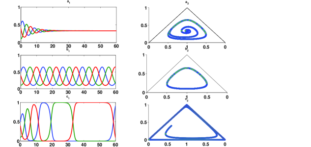
Figure 5: The feedback interconnection between the three different scenarios of rock paper scissors game (21) and the standard replicator dynamics (18) projected into the simplex.

.

IV-B Distributed Replicator Dynamics

Generally, the stranded Replicator dynamics describes the dynamics of the deterministic limit of an infinitely large, well-mixed population, where the spatial effects are not considered. Here, ‘Well-mixed’ indicate that there is no particular structure imposed into the game. In other words, all agents are equally likely to interact with one another. This can be represented as a fully connected graph (complete graph) [33].

However, in structured populations (non-well mixed populations), the individual agents set on the vertices of a graph and the edges of determine which agents interact with each other [33]. This scenario is called distributed Replicator dynamics in [34]. Also, it is called local Replicator dynamics in [35]. The distributed (or local) Replicator dynamics is represented as follows:

$$\dot{x_{i}}=x_{i}(p_{i}\sum_{j\in N_{i}}x_{j}-\sum_{j\in N_{i}}x_{j}p_{j}),$$ (22)

meant to models the inference of population dynamics that involve non-well mixed populations.

In the case where the payoff $P=Ax$, the stander replicator dynamics with can be written as follows;

$$\dot{x_{i}}=x_{i}\left((Ax)_{i}-x^{T}Ax\right),$$ (23)

In [36] evolutionary models for infinite and finite populations: While the population itself is infinite, interactions and reproduction occurs in random groups of size $N$. This leads to a modified payoff matrix in the following form:

$$A_{new}=A-\frac{A+A^{T}}{N}$$ (24)

Therefore, the local replicator dynamics is given as follows;

$$\dot{x_{i}}=x_{i}\left((A_{new}x)_{i}-x^{T}A_{new}\;x\right),$$ (25)

The following proposition shows that the local replicator dynamics is also lossless passive from the error to the payoff.

Proposition 1

The local replicator dynamics defined in (25) from the error $e_{x_{i}}$ to the payoff $P=Ax$ is lossless passive.

Proof:

Using $e_{x_{i}}=x_{i}-x^{*}_{i}$, the replicator dynamic equation (25) can be written as follows:

$$\dot{e}_{x_{i}}= (e_{x_{i}}+x^{*}_{i})[(A_{new}(e_{x}+x^{*}))_{i}$$ (26)

$$-(e_{x}+x^{*})^{T}\;A_{new}\;(e_{x}+x^{*})].$$ (27)

Define the following storage function,

$$V(e_{x})=-\left(\frac{N}{N-2}\right)\sum_{i}x^{*}_{i}\ln\frac{e_{x_{i}}+x^{*}_{i}}{x^{*}_{i}}.$$ (28)

Note that $V(0)=0$, and

$$V(e_{x}) =-\left(\frac{N}{N-2}\right)\sum_{i}x^{*}_{i}\ln\frac{e_{x_{i}}+x^{*}_{i}}{x^{*}_{i}}$$

$$\geq-\left(\frac{N}{N-2}\right)\ln\sum_{i}x^{*}_{i}\frac{e_{x_{i}}+x^{*}_{i}}{x^{*}_{i}}$$

$$=\left(\frac{N}{N-2}\right)\ln(\sum_{i}x_{i}),$$

However, $\sum_{i}x_{i}=1$. It follows that $V(e_{x})\geq 0$.

Now, the derivative of the storage function is given as follows:

$$\dot{V}(e_{x})$$

$$=-\left(\frac{N}{N-2}\right)\sum_{i}x^{*}_{i}\frac{1}{e_{x_{i}}+x^{*}_{i}}\dot{e}_{x_{i}}$$

$$=-\left(\frac{N}{N-2}\right)\sum_{i}x^{*}_{i}[(A_{new}(e_{x}+x^{*}))_{i}$$

$$\;\;\;\;\;\;\;\;\;\;\;\;\;-(e_{x}+x^{*})^{T}\;A_{new}\;(e_{x}+x^{*})]$$

$$=-\left(\frac{N}{N-2}\right)[x^{*T}A_{new}(e_{x}+x^{*})$$

$$\;\;\;\;\;\;\;\;\;\;\;\;\;-(e_{x}+x^{*})^{T}\;A_{new}\;(e_{x}+x^{*})]$$

$$=-\left(\frac{N}{N-2}\right)[x^{*T}A_{new}e_{x}+x^{*T}A_{new}x^{*}-e_{x}^{T}A_{new}e_{x}$$

$$\;\;\;\;\;\;\;\;-e_{x}^{T}\;A_{new}\;x^{*}-x^{*T}\;A_{new}\;e_{x}-x^{*T}A_{new}x^{*}]$$

$$=-\left(\frac{N}{N-2}\right)[-e_{x}^{T}A_{new}e_{x}-e_{x}^{T}\;A_{new}\;x^{*}]$$

$$=\left(\frac{N}{N-2}\right)e_{x}^{T}A_{new}(e_{x}+x^{*})$$

$$=\left(\frac{N}{N-2}\right)e_{x}^{T}\left(A-\frac{A+A^{T}}{N}\right)x$$

$$=\left(\frac{N}{N-2}\right)\left(e_{x}^{T}Ax-\frac{1}{N}(e_{x}^{T}Ax+e_{x}^{T}A^{T}x)\right)$$

$$=\left(\frac{N}{N-2}\right)\left(e_{x}^{T}Ax-\frac{2}{N}e_{x}^{T}Ax\right)$$

$$=\left(\frac{N}{N-2}\right)\left(1-\frac{2}{N}\right)e_{x}^{T}Ax$$

$$=e_{x}^{T}Ax$$

$$=e_{x}^{T}P$$

This implies that replicator dynamics are passive (lossless) system. ∎

IV-C Second order replicator dynamics

Second order dynamics can be introduced into the evolutionary dynamics through several forms [37, 15]. In this section, we follow the approach in [15], which use an auxiliary state to introduce the Second order dynamics to derive two versions of the Second order replicator dynamics.

IV-C1 Integral action Second order replicator dynamics

One form of the second order replicator dynamics can be obtained by introducing an auxiliary state $\widehat{p}$ in the payoff function. This results in the following dynamics:

$$\dot{x_{i}} =x_{i}(\widehat{p}_{i}-\sum_{j}x_{j}\widehat{p}_{j})$$ (29a)

$$\dot{\widehat{p}_{i}} =p_{i}.$$ (29b)

The equilibrium conditions are $p_{i}^{*}=0$, $x_{i}^{*}=\sigma_{\text{max}}(\widehat{p}_{i}^{*})$, and $\widehat{p}_{i}^{*}=1$ .

The Equation (29b) can be written as follows;

$$\dot{\widehat{p}_{i}} =p_{i}$$ (30)

$$\widehat{p}_{i} =\int_{0}^{t}p_{i}(\tau)d\tau.$$ (31)

It has been shown in [38] that the second order replicator dynamics is not passive. In particular, it has been shown that the linearization of the replicator dynamics (29) is reduced to a double integrator, which is not passive.

The following proposition proves that the second order replicator defined in (29) is a negative imaginary system according to the definition given in (6).

Proposition 2

The second order replicator dynamics defined in (29) from the error $e_{x_{i}}$ to the payoff $P$ is a negative imaginary system.

Proof:

Using $e_{x_{i}}=x_{i}-x^{*}_{i}$, the replicator dynamic equation (29) can be written as follows:

$$\dot{e}_{x_{i}} =(e_{x_{i}}+x^{*}_{i})(\widehat{p_{i}}-\sum_{j}(e_{x_{j}}+x^{*}_{j})\widehat{p_{j}})$$ (32)

$$\widehat{p}_{i} =\int_{0}^{t}p_{i}(\tau)d\tau.$$ (33)

Using the storage function (20), it follows that;

$$\dot{V}(e_{x}) =-\sum_{i}x^{*}_{i}\frac{1}{e_{x_{i}}+x^{*}_{i}}\dot{e}_{x_{i}}$$

$$=-\sum_{i}x^{*}_{i}(\widehat{p_{i}}-\sum_{j}(e_{x_{j}}+x^{*}_{j})\widehat{p_{j}})$$

$$=-\sum_{i}x^{*}_{i}\widehat{p_{i}}+\sum_{i}x^{*}_{i}(\sum_{j}e_{x_{j}}\widehat{p_{j}}+\sum_{j}x^{*}_{j}\widehat{p_{j}})$$

$$=-\sum_{i}x^{*}_{i}\widehat{p_{i}}+\sum_{j}e_{x_{j}}\widehat{p_{j}}+\sum_{j}x^{*}_{j}\widehat{p_{j}}$$

$$=\sum_{j}e_{x_{j}}\widehat{p_{j}}$$

$$=\sum_{j}e_{x_{j}}\int_{0}^{t}p_{j}(\tau)d\tau.$$

This implies that second order replicator dynamic is negative imaginary. ∎

It is straightforward to show that the linearization of the replicator dynamics around an equilibrium point, which is given as

$$\delta\dot{x} =A\delta x+\beta\delta\widehat{p}$$

$$\delta\dot{\widehat{p}} =\delta p,$$

satisfies the negative imaginary property. Here, $A=\begin{bmatrix}-x_{1}^{*}&-x_{1}^{*}&\cdots&-x_{1}^{*}\\ -x_{2}^{*}&-x_{2}^{*}&\cdots&-x_{2}^{*}\\ \vdots&\vdots&\vdots&\vdots\\ -x_{n}^{*}&-x_{n}^{*}&\cdots&-x_{n}^{*}\end{bmatrix}$, $\beta=I-x^{*}x^{*T}$ and $x^{*}$ is any point in the simplex. The reduced system can be obtained using the transformation $\delta x=\delta x^{*}+N\delta w$, $\delta p=\delta p^{*}+N\delta q$ and $\delta\widehat{p}=N\xi$ as follows:

$$\delta\dot{w} =N^{T}AN\delta w+N^{T}\beta N\xi$$

$$\dot{\xi} =\delta q.$$

Now, consider the case where $n=3$ and $x_{i}^{*}=\frac{1}{3}$,

$$\begin{bmatrix}\delta\dot{w}\\ \dot{\xi}\end{bmatrix} =\begin{bmatrix}0&0&1&0\\ 0&0&0&1\\ 0&0&0&0\\ 0&0&0&0\end{bmatrix}\begin{bmatrix}\delta w\\ \xi\end{bmatrix}+\begin{bmatrix}0&0\\ 0&0\\ 1&0\\ 0&1\end{bmatrix}\delta q$$ (34a)

$$\delta y =\begin{bmatrix}1&0&0&0\\ 0&1&0&0\end{bmatrix}\begin{bmatrix}\delta w\\ \xi\end{bmatrix}.$$ (34b)

The system (34) is a double integrator, which is a negative imaginary system.

Proposition 2 shows that the second order replicator dynamics defined in (29) satisfies the negative imaginary property. This implies that the feedback interconnection between the second order replicator dynamics defined in (29) and any strictly negative imaginary game should lead to a stable behaviour [30].

For instance, consider the following second order negative imaginary game;

$$\dot{z} =Az+B\;u$$

$$P =Cz+D\;u,$$ (35)

where,

$$A =\begin{bmatrix}-0.9&0\\ 0&-1.2\end{bmatrix},B=\begin{bmatrix}1&0\\ 0&1\end{bmatrix},$$

$$C =\begin{bmatrix}1&0\\ 0&1\end{bmatrix}\text{ and }D=\begin{bmatrix}-3&0\\ 0&-3\end{bmatrix}.$$

The feedback interconnection between the second order replicator dynamics (29) and the second order strictly negative imaginary game (35) is demonstrated in Fig. reffig:RD-g and Fig. 7.

Figs. 6 and 7 shows the evolution of the states of the positive feedback interconnection between the strictly negative imaginary game (35) and second order replicator dynamic (29).

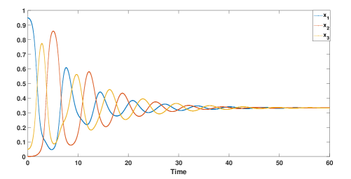
Figure 6: The evolution of the states of the strictly negative imaginary game (35) in feedback loop with the second order replicator dynamics (29).

.

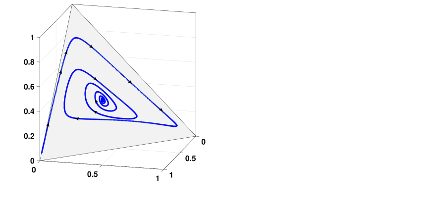
Figure 7: The evolution of the states of the strictly negative imaginary game (35) in feedback loop with the second order replicator dynamics (29) projected into the simplex.

.

IV-C2 Lead-lag second order replicator dynamics

A more general second order replicator dynamics can be introduced using derivative action combined with low pass filter as a prepossessing to the payoffs before the replicator dynamics as shown in Fig. 8. The Lead-lag second order replicator dynamics can be defined using an auxiliary state $\widehat{p}$. The dynamics is given as follows;

$$\dot{x_{i}} =x_{i}(y_{i}-\sum_{j}x_{j}y_{j})$$ (36a)

$$\dot{\widehat{p}_{i}} =\frac{-1}{\beta}\widehat{p}+p_{i}$$ (36b)

$$y_{i} =(\frac{1}{\beta}-\frac{\alpha}{\beta^{2}})\widehat{p}+\frac{\alpha}{\beta}p_{i}.$$ (36c)

Here, $\alpha$ and $\beta$ are positive constants.

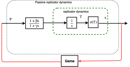
Figure 8: Passive replicator dynamics.

.

The passivity propriety of second order replicator dynamics given in (36) depends on the ratio between the constants $\alpha$ and $\beta$. The following preposition discuss the passivity property of the replicator dynamics given in (36).

Proposition 3

The second order replicator dynamics given in (36) is negative imaginary for all positive constant $\alpha$ and $\beta$ and passive if and only if $\frac{\alpha}{\beta}>1$.

Proof:

The dynamical part of the second order replicator dynamic given in (36) can be expressed as a serial connection between an integrator, $\frac{1}{s}$, and the following transfer function

$$\frac{1+\alpha\;s}{1+\beta\;s}.$$

In other words, the dynamical part of second order replicator dynamic given in (36) in frequency domain is given as follows;

$$G_{RD}(j\omega)=\frac{1+\alpha\;j\omega}{j\omega\;(1+\beta\;j\omega)}.$$ (37)

The real and imaginary part of the transfer function (37) is given as follows;

$$\Re(G_{RD})=\frac{\beta(\alpha/\beta-1)}{\beta^{2}\omega^{2}+1}.$$ (38)

$$\Im(G_{RD})=\frac{-(\alpha\beta\omega^{2}+1)}{\beta^{2}\omega^{3}+\omega}.$$ (39)

It is clear from (38) that the real part of $G_{RD}(j\omega)$ is positive if and only if $\frac{\alpha}{\beta}>1$. Also, (39) shows that the imaginary part is always negative for all positive $\alpha$ and $\beta$.

∎

Fig. 9 demonstrates the feedback interconnection between the standard rock paper scissors game (21) with $w=l$, i.e., lossless game and the second order replicator dynamics given (36). The top figure in Fig. 9 represents the non-passive replicator dynamics where $\frac{\alpha}{\beta}<1$, where the bottom figure represents the passive replicator dynamics with $\frac{\alpha}{\beta}>1$ .

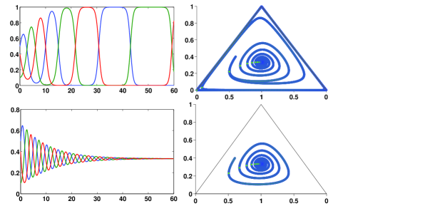
Figure 9: The evolution of the states of the strictly negative imaginary game (35) in feedback loop with the second order replicator dynamics (29).

.

V Passivation of non-passive dynamics

This section introduces the notion of passivation thorough a feedback or forwarded of non-passive dynamics and static gain. The term passivation in passivity theory means the process of forcing a non-passive or lossless dynamical system to behave as a strictly passive system using feedback and/or foreword interconnection. Similarly,

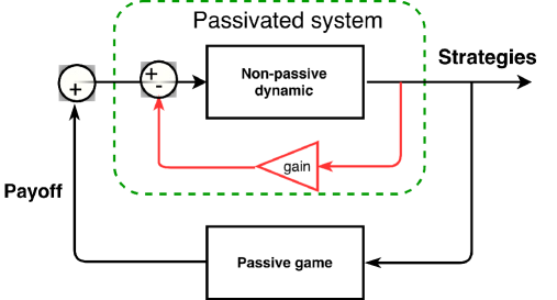
Figure 10: Passiviation of lossless or non-passive dynamics throgh static feedback gain. Here, the static gain is chosen to passivate the dynamics in the colored green box.

.

In the case of replicator dynamics, any positive gain in negative feedback interconnection will change the replicator dynamics for lossless dynamics to strictly passive dynamics in Fig. 11.

Figure 11: Passive replicator dynamics.

.

The passive first order replicator dynamics is then given as follows;

$$\dot{x_{i}} =x_{i}(\dot{T_{i}}-\sum_{j}x_{j}\dot{T_{j}})$$

$$\dot{T_{i}} =P_{i}-K_{i}x_{i}.$$ (40)

Similarly, as in Proposition 3, we can show that the modified replicator dynamics (V) a is strictly passive.

VI Concluding Remarks

In this paper, passivity analysis for different versions of the replicator dynamics was conducted. The standard first order replicator dynamics is shown to be passive lossless. This implies that the replicator dynamics will lead to a stable equilibrium with all strictly passive games. Similarly, the second order replicator dynamics is shown to satisfy the negative imaginary property, which implies that the second order replicator dynamics leads to a stable equilibrium with all strictly negative imaginary games.

Dr. Mohamed A. Mabrok is an Assistant Professor with the Faculty of Engineering at the Australian College of Kuwait. In 2004 he obtained a bachelor degree applied mathematics and computer science and in 2009 he obtained a masters degree in applied mathematics and quantum physics. In 2013, Dr. Mabrok obtained his Ph.D., in electrical engineering in the field of robust control theory from the University of New South Wales, Australia, with Professor Ian Petersen. After finishing his Ph.D., Dr. Mabrok worked as a postdoctoral fellow at the the UNSW at the Australian Defence Force Academy for two years. In 2015, he joined professor Jeff Shamma’ group at KAUST as a postdoctoral fellow for two years. In 2017, he joined the Australian College of Kuwait as an assistant professor. Dr. Mabrok’s main research interests and experience are in robust control theory, game theoretic learning, quantum control theory, and Human in the loop control.

References

- [1] W. H. Sandholm, Population Games and Evolutionary Dynamics. MIT Press, 2010.
- [2] J. Hofbauer and K. Sigmund, Evolutionary Games and Population Dynamics. Cambridge, UK: Cambridge University Press, 1998.
- [3] H. P. Young, Individual Strategy and Social Structure. Princeton, NJ: Princeton University Press, 1998.
- [4] J. M. Smith, Evolution and the Theory of Games. Cambridge University Press, 1982.
- [5] J. Marden and J. S. Shamma, “Game theory and distributed control,” in Handbook of Game Theory, H. P. Young and S. Zamir, Eds. North-Holland, 2015, vol. 4, pp. 861–899.
- [6] D. Fudenberg and D. Levine, The Theory of Learning in Games. Cambridge, MA: MIT Press, 1998.
- [7] S. Hart, “Adaptive heuristics,” Econometrica, vol. 73, no. 5, pp. 1401–1430, 2005.
- [8] H. P. Young, Strategic Learning and its Limits. Oxford University Press, 2005.
- [9] J. Hofbauer and K. Sigmund, “Evolutionary game dynamics,” Bulletin of the American Mathematical Society, vol. 40, no. 4, pp. 479–519, 2003.
- [10] J. Hofbauer and W. H. Sandholm, “Stable games and their dynamics,” Journal of Economic Theory, vol. 144, no. 4, pp. 1665–1693, 2009.
- [11] S. Hart and A. Mas-Colell, “Uncoupled dynamics do not lead to Nash equilibrium,” American Economic Review, vol. 93, no. 5, pp. 1830–1836, 2003.
- [12] P. D. Taylor and L. B. Jonker, “Evolutionary stable strategies and game dynamics,” Mathematical biosciences, vol. 40, no. 1-2, pp. 145–156, 1978.
- [13] P. Schuster and K. Sigmund, “Replicator dynamics,” Journal of Theoretical Biology, vol. 100, no. 3, pp. 533–538, 1983.
- [14] R. Cressman and Y. Tao, “The replicator equation and other game dynamics,” Proceedings of the National Academy of Sciences, vol. 111, no. Supplement 3, pp. 10 810–10 817, 2014.
- [15] M. J. Fox and J. S. Shamma, “Population games, stable games, and passivity,” Games, vol. 4, no. 4, pp. 561–583, 2013.
- [16] S. Sato, E. Akiyama, and J. D. Farmer, “Chaos in learning a simple two person game,” Proceedings of the National Academy of Sciences, vol. 99, no. 7, pp. 4748–4751, 2002.
- [17] J. S. Shamma and G. Arslan, “Dynamic fictitious play, dynamic gradient play, and distributed convergence to nash equilibria,” IEEE Transactions on Automatic Control, vol. 50, no. 3, pp. 312–327, 2005.
- [18] G. Arslan and J. S. Shamma, “Anticipatory learning in general evolutionary games,” in 45th IEEE Conference on Decision and Control, San Diego, CA, December 2006, pp. 6289–6294.
- [19] R. Laraki and P. Mertikopoulos, “Higer order game dynamics,” Journal of Economic Theory, vol. 148, no. 6, pp. 2666–2695, 2013.
- [20] R. Lozano, B. Brogliato, O. Egeland, and B. Maschke, Dissipative Systems Analysis and Control: Theory and Applications. SpringerScience & Business Media, 2013.
- [21] J. C. Willems, “Dissipative dynamical systems part I: General theory,” Archive for Rational Mechanics and Analysis, vol. 45, no. 5, pp. 321–351, 1972.
- [22] A. V. der Schaft, L2-Gain and Passivity Tecniques in Nonlinear Control. Springer Science & Business Media, 2012.
- [23] A. Lanzon and I. R. Petersen, “Stability robustness of a feedback interconnection of systems with negative imaginary frequency response,” IEEE Transactions on Automatic Control, vol. 53, no. 4, pp. 1042–1046, 2008.
- [24] I. R. Petersen and A. Lanzon, “Feedback control of negative imaginary systems,” IEEE Control System Magazine, vol. 30, no. 5, pp. 54–72, 2010.
- [25] J. Xiong, I. R. Petersen, and A. Lanzon, “A negative imaginary lemma and the stability of interconnections of linear negative imaginary systems,” IEEE Transactions on Automatic Control, vol. 55, no. 10, pp. 2342–2347, 2010.
- [26] M. Mabrok, M. Haggag, I. Petersen, and A. Lanzon, “A subspace system identification algorithm guaranteeing the negative imaginary property,” in Decision and Control (CDC), 2014 IEEE 53rd Annual Conference on. IEEE, 2014, pp. 3180–3185.
- [27] M. A. Mabrok, M. Efatmaneshnik, and M. Ryan, “Including non-functional requirements in the axiomatic design process,” in Systems Conference (SysCon), 2015 9th Annual IEEE International. IEEE, 2015, pp. 54–60.
- [28] A. G. G. M. A. M. and Ian R. Petersen, “Extending negative imaginary systems theory to nonlinear systems,” 2018.
- [29] M. Mabrok, A. Kallapur, I. Petersen, and A. Lanzon, “Generalizing negative imaginary systems theory to include free body dynamics: Control of highly resonant structures with free body motion,” Automatic Control, IEEE Transactions on, vol. 59, no. 10, pp. 2692–2707, Oct 2014.
- [30] M. A. Mabrok, A. G. Kallapur, I. R. Petersen, and A. Lanzon, “A stability result on the feedback interconnection of negative imaginary systems with poles at the origin,” in Proceedings of the 2012 Australian Control Conference, Sydney, Australia, 2012.
- [31] K. Zhou, J. C. Doyle, and K. Glover, Robust and Optimal Control. Upper Saddle River, NJ: Prentice-Hall, Inc., 1996.
- [32] K. J. Arrow, Social choice and individual values. Yale university press, 1963, no. 12.
- [33] H. Ohtsuki and M. A. Nowak, “The replicator equation on graphs,” Journal of theoretical biology, vol. 243, no. 1, pp. 86–97, 2006.
- [34] G. D. O. Bravo, “Distributed methods for resource allocation: a passivity based approach,” Ph.D. dissertation, Ecole des Mines de Nantes, 2015.
- [35] A. Pantoja, N. Quijano, and K. M. Passino, “Dispatch of distributed generators using a local replicator equation,” in Decision and Control and European Control Conference (CDC-ECC), 2011 50th IEEE Conference on. IEEE, 2011, pp. 7494–7499.
- [36] C. Hilbe, “Local replicator dynamics: a simple link between deterministic and stochastic models of evolutionary game theory,” Bulletin of mathematical biology, vol. 73, no. 9, pp. 2068–2087, 2011.
- [37] R. Laraki and P. Mertikopoulos, “Higher order game dynamics,” Journal of Economic Theory, vol. 148, no. 6, pp. 2666–2695, 2013.
- [38] M. Mabrok and J. S. Shamma, “Passivity analysis of higher order evolutionary dynamics and population games,” in Decision and Control (CDC), 2016 IEEE 55th Conference on. IEEE, 2016, pp. 6129–6134.