Code O-SUKI: Simulation of Direct-Drive Fuel Target Implosion in Heavy Ion Inertial Fusion

Abstract

The Code O-SUKI is an integrated 2-dimensional (2D) simulation program system for a fuel implosion, ignition and burning of a direct-drive nuclear-fusion pellet in heavy ion beam (HIB) inertial confinement fusion (HIF). The Code O-SUKI consists of the four programs of the HIB illumination and energy deposition program of OK3 (Comput. Phys. Commun. 181, 1332 (2010)), a Lagrangian fluid implosion program, a data conversion program, and an Euler fluid implosion, ignition and burning program. The OK3 computes the multi-HIBs irradiation onto a spherical fuel target. One HIB is divided into many beamlets in OK3. Each heavy ion beamlet deposits its energy along the trajectory in a deposition layer depending on the particle energy. The OK3 also has a function of a wobbling motion of the HIB axis oscillation, and the HIBs energy deposition spatial detail profile is obtained inside the energy absorber of the fuel target. The spherical target implosion 2D behavior is computed by the 2D Lagrangian fluid code coupled with OK3, until just before the void closure time of the fuel implosion. After that, all the data by the Lagrangian implosion code are converted to them for the Eulerian code. The fusion Deuterium (D)-Tritium (T) fuel and the inward moving heavy tamping material are imploded and deformed seriously at the stagnation phase. The Euler fluid code is appropriate to simulate the fusion fuel compression, ignition and burning. The Code O-SUKI 2D simulation system provides a capability to compute and to study the HIF target implosion dynamics.

Program summary

Program Title: O-SUKI
Licensing provisions: CC BY NC 3.0
Programming language: C++
Computer: PC(Pentium 4, 1 GHz or more recommended)
RAM: 3072 MBytes
Operating system: UNIX
Journal reference of previous version: No
Nature of problem: The nuclear fusion energy would provide one of energy resources for our human society. In this paper we focus on heavy ion beam (HIB) inertial confinement fusion (HIF). A spherical deuterium (D) - tritium (T) fuel pellet, whose radius may be about several mm, is irradiated by HIBs to be compressed to about a thousand times of the solid density. The DT fuel temperature reaches $\sim$5-10KeV to be ignited to release the DT fusion energy. The typical HIBs total input energy is several MJ, and the HIBs pulse length is about a few tens of ns. The DT fuel compression uniformity is essentially important to release the sufficient fusion energy output. The DT fuel pellet implosion non-uniformity should be kept less than a few %. The O-SUKI code system provides an integrated tool to simulate the HIF DT fuel pellet implosion, ignition and burning. The HIBs energy deposition detail profile is computed by the OK3 code (Comput. Phys. Commun. 181, 1332 (2010)) in an energy absorber outer layer, which covers the DT fuel spherical shell. The DT fuel is compressed to the high density, and so the DT fuel spatial deformation may be serious at the DT fuel stagnation. Therefore, the O-SUKI system employs a Lagrangian fluid code first to simulate the DT fuel implosion phase until just before the stagnation. Then all the simulation data from the Lagrangian code are converted to them for the Euler fluid code, in which the DT fuel ignition and burning are simulated.
Solution method: In the two fluids codes (Lagrangian and Euler fluid codes) in the O-SUKI system the three-temperature fluid model (J. Appl. Phys. 60, 898 (1986)) is employed to simulate the pellet dynamics in HIF. The HIBs energy deposition detail profile is computed by the OK3 code (Comput. Phys. Commun. 181, 1332 (2010)).
Additional comments including Restrictions and Unusual features: No

1 Introduction

In inertial confinement fusion (ICF) a deuterium (D) - tritium (T) fuel target implosion, ignition and burning are essentially important to release a sufficient fusion energy output. In the nuclear fusion two nuclei of D and T are fused once. The DT fusion reaction creates He and neutron, and releases the energy of the mass defect as their kinetic energy in the DT reaction. In ICF a few mg DT in a fuel pellet is first heated up to $\sim$5-10KeV by an input driver energy, for example, lasers or heavy ion beams (HIBs) or pulse power [1]. Especially, the solid DT fuel density must be compressed to about a thousand times of the solid density to reduce the input energy and also to realize controlled fusion reactions. In addition, the ion temperature of the compressed DT must reach $\sim$5-10 KeV. In order to compress the DT fuel stably to the high density, the implosion non-uniformity should be less than a few percent[2] The central issues of the fuel implosion in ICF includes how to realize the uniform implosion, how we can control the driver beam energy deposition to compress the DT fuel to the high density, and consequently how to keep the implosion stable during the fuel implosion. The O-SUKI code system provides an integrated computer simulation tool to study the DT fuel implosion, ignition and burning in heavy ion inertial confinement fusion (HIF).

The heavy ion beam (HIB) fusion has been proposed in 1970s. The recent HIF activities and reviews are found in Refs. [3, 4]. The HIF reactor designs were also proposed[5, 6, 7]. HIB ions deposit their energy inside of materials, and the interaction of the HIB ions with the materials are well understood [8, 9]. The HIB ion interaction with a material is explained and defined well by the classical Coulomb collision and a plasma wave excitation in the material plasma. The HIB ions deposit all the HIB ion energy inside of the material. The HIB energy deposition length is typically the order of $\sim$mm in an HIF fuel target depending on the HIB ion energy and the material. When several MJ of the HIB energy is deposited in the material in an inertial confinement fusion (ICF) fuel target, the temperature of the energy deposition layer plasma becomes about 300 eV or so. The peak temperature or the peak plasma pressure appears near the HIB ion stopping area by the Bragg peak effect, which comes from the nature of the Coulomb collision. The total stopping range would be normally wide and the order of $\sim$mm inside of the material. An indirect drive target was also proposed in Ref. [10].

In ICF, a driver efficiency and its repetitive operation with several Hz $\sim$ 20 Hz or so are essentially important to constitute an ICF reactor system. HIB driver accelerators have a high driver energy efficiency of $\sim$30-40 % from the electricity to the HIB energy. In general, high-energy accelerators have been operated repetitively daily. The high driver efficiency relaxes the requirement for the fuel target gain. In HIF the target gain of 30$\sim$50 allows us to construct a HIF fusion reactor system, and 1MkW of the electricity output would be realized with the repetition rate of $\sim$10$\sim$15 Hz.

The HIB accelerator also has a high controllability to define the ion energy, the HIB pulse shape, the HIB pulse length and the HIB number density or current as well as the beam axis. The HIB axis could be also controlled or oscillated with a high frequency[11, 12, 13]. The controlled wobbling motion of the HIB axis is one of remarkable preferable points in HIF, and would contribute to smooth the HIBs illumination non-uniformity on a DT fuel target and to mitigate the Rayleigh-Taylor (R-T) instability growth in the HIF fuel target implosion[14, 15, 16]. In the OK3 code the HIBs wobbling capability is also installed to study the wobbling ion beam energy deposition.

The relatively large density gradient scale length is created in the HIBs energy deposition region in an DT fuel target, and it also contribute to reduce the R-T instability growth rate especially for shorter wavelength modes[17, 18]. So in the HIF target implosion longer wavelength modes should be focused for the target implosion uniformity.

In general the target implosion non-uniformity is introduced by a driver beams’ illumination non-uniformity, an imperfect target sphericity, a non-uniform target density, a target alignment error in a fusion reactor, et al. The target implosion should be also robust against the implosion non-uniformities for the stable reactor operation.

In the HIBs energy deposition region in a DT fuel target a wide density valley appears, and in the density valley a part of the HIBs deposited energy is converted to the radiation and the radiation is confined in the density valley [19]. The converted and confined radiation energy is not negligible, and it would be the order of $\sim$100 kJ in a HIF reactor-size DT target. The confined radiation in the density valley contributes also to reduce the non-uniformity of the HIBs energy deposition.

The HIB uniform illumination was also studied, and the target implosion uniformity requirement requests the minimum HIB number: details HIBs energy deposition on a direct-drive DT fuel target shows that the minimum HIBs number would be the 32 beams [20]. The detail HIBs illumination on a HIF DT target is computed by a computer code of OK3 [21, 22, 23]. The HIBs illumination non-uniformity is also studied in detail. One of the study results shows that a target misalignment of $\sim$100$\mu$m is tolerable in fusion reactor to release the HIF energy stably.

The DT fuel implosion is simulated until just before the void closure time by the Lagrangian code, which couples with the OK3 code to include the time-dependent HIBs energy deposition profile in the target energy absorber layer. The Lagrange code data are converted to the data imported to the Euler code, which is robust against the target fuel and material deformation. The DT fuel ignition and burning are simulated further by the Euler fluid code. The O-SUKI code system simulates the 2D HIF target implosion dynamics, and would contribute to release the fusion energy stably and in a robust way for our human society.

2 O-SUKI code algorithm description

2.1 O-SUKI code structure

The O-SUKI code system is an integrated DT fuel implosion code in HIF, and consists of four parts: The HIBs illumination code of OK3 [23], the Lagrangian fluid code [24], the data conversion code from the Lagrangian code to the Euler code, and Euler code. The fluid model is the three-temperature model in Ref. [25]. The detail information on OK3 is presented in Refs. [21, 22, 23]. The Lagrangian fluid code, the data conversion code and the Euler code are described below in detail.

In the Lagrangian fluid code the spatial meshes move together with the fluid motion [24]. However the mass and energy conservations are well described, the Lagrange meshes can not follow the fluid large deformation. On the other hand, the Euler meshes are fixed to the space, and the fluid moves through the meshes. Therefore, just before the void closure time, that is, the stagnation phase, the Lagrangian code is used to simulate the DT fuel implosion. After the void closure time, the Euler code is employed to simulate the DT fuel further compression, ignition and burning. Between the Lagrangian code and the Euler code the data should be converted by the data conversion code.

All the simulation process is performed in its integrated way by using the script of ”O-SUKIcode_start.sh”. The processes executed by this shell script are as follows.
1. Make the stack size infinite.
2. Change the permission of shell scripts to executable.
3. Compile the main function of the Lagrangian code and execute it.
4. If any problems do not appear during the calculation of the Lagrangian code, compile the main function of the data conversion code and execute it.
5. If there is no problem during the data conversion, compile the main function of the Euler code and execute it.

2.2 Steps in Lagrangian code

The Lagrangian code has the following steps:

1. Initialize the variables.

2. Calculation of time step size.

3. Calculation of coordinates.

4. Solve equation of motion.

5. Solve density by equation of continuity.

6. Calculation of artificial viscosity.

7. Transfer the data to the OK3.

8. Calculation of energy deposition distribution in code OK3. For details of the OK3, see the ref.[21, 22, 23].

9. Solve energy equations

10. Calculation of heat conduction

11. Calculation of temperature relaxation among three temperatures.

12. Solve equation of state

13. Save the results.

14. End the Lagrangian calculation right before the void closure.

15. Transfer the data to converting code.

2.3 Data Conversion code from Lagrangian fluid code to Euler fluid code

1. Read variables saved in Lagrangian code.

2. Generate the Eulerian mesh.

3. Calculate the interpolation of the physical quantity to them on the Eulerian mesh.

4. Write the converted data to the Eulerian code.

2.4 Steps in Eulerian code

1. Read the mesh number from the converted data and define the each matrices.

2. Initialize the variables.

3. Calculation of time step size.

4. Solve equation of motion.

5. Track the material boundaries of DT, Al and Pb.

6. Linearly interpolate the boundary lines and transcribe them on the Eulerian code.

7. Discriminate the materials by using the transferred boundary line.

8. Solve density by equation of continuity.

9. Calculate artificial viscosity.

10. Solve energy equations

11. Calculation of fusion reaction.

12. Calculation of heat conduction

13. Calculation of temperature relaxation among three temperatures.

14. Solve equation of state.

15. Save the results.

16. End.

3 Included files

The coordinates in the Lagrangian fluid simulation code are as shown below (see Fig. 1)．The discretization method in Ref. [24] is employed in the Lagrangian fluid code.

$$R=R(k,l,t)$$

$$Z=Z(k,l,t)$$

The position vector ${\bm{R}}$ and the vector ${\bar{\bm{R}}}$ are introduced as follows.

$${\bm{R}}=\begin{bmatrix}R\\ Z\end{bmatrix}\ ,\ {\bar{\bm{R}}}=\begin{bmatrix}Z\\ -R\end{bmatrix}$$

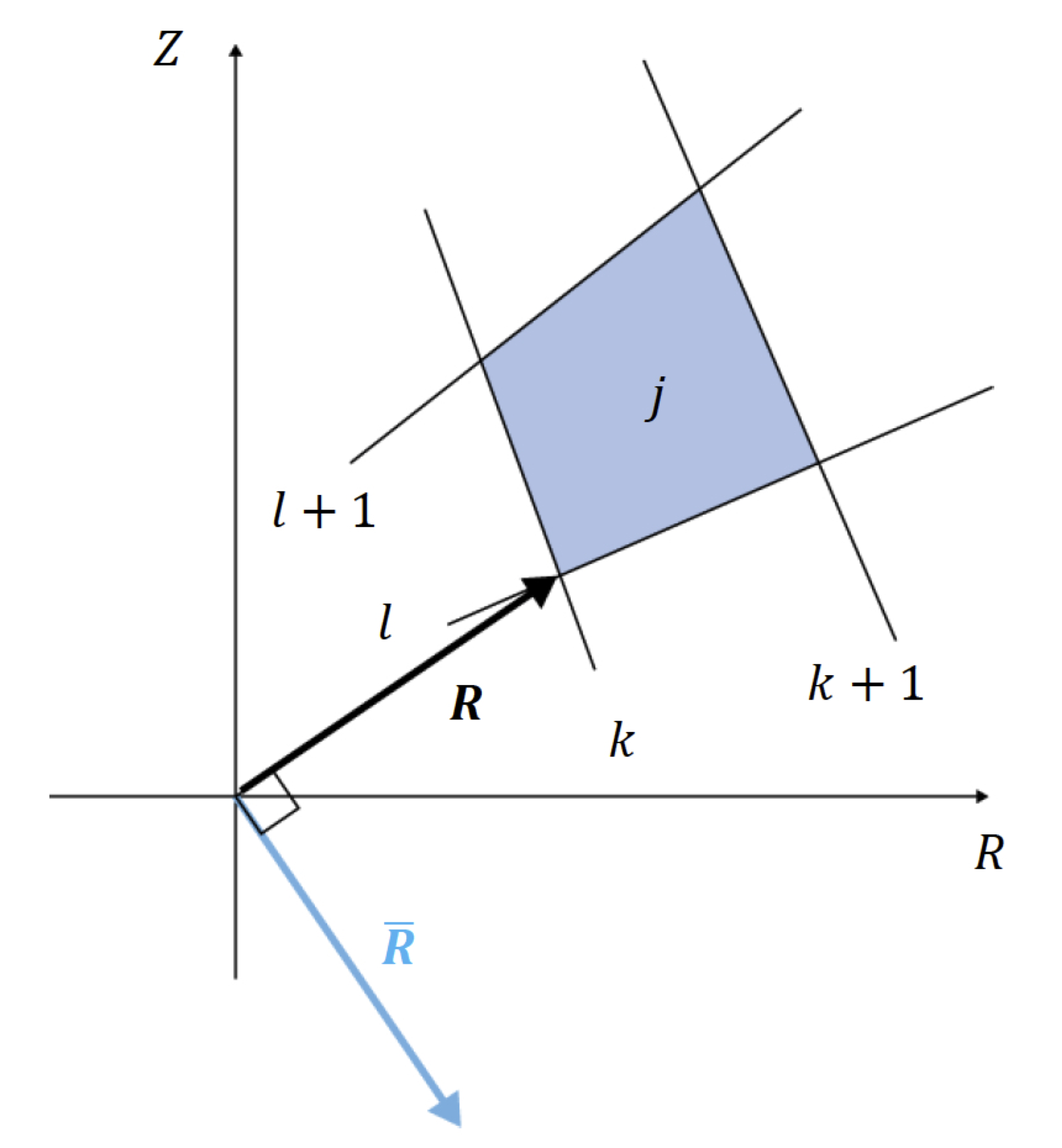
Figure 1: Lagrangian coordinate.

The definition points of the discretized physical quantities in the Lagrange and Euler codes are presented in Figs. 2 and 3, respectively. The subscripts $k$ and $l$ correspond to the positions in space, and the subscript $n$ corresponds to time $n\times dt$. The displacement amounts in the $k$ and $l$ directions are defined as follows.

$$dR^{n}_{k+\frac{1}{2},l}=R^{n}_{k+1,l}-R^{n}_{k,l}$$ (1)

$$dZ^{n}_{k,l+\frac{1}{2}}=Z^{n}_{k,l+1}-Z^{n}_{k,l}$$ (2)

$$\begin{cases}\Delta R^{n}_{k+\frac{1}{2},l}=R^{n}_{k+1,l}-R^{n}_{k,l}\\ \delta R^{n}_{k,l+\frac{1}{2}}=R^{n}_{k,l+1}-R^{n}_{k,l}\end{cases}$$

$$\begin{cases}\Delta Z^{n}_{k+\frac{1}{2},l}=Z^{n}_{k+1,l}-Z^{n}_{k,l}\\ \delta Z^{n}_{k,l+\frac{1}{2}}=Z^{n}_{k,l+1}-Z^{n}_{k,l}\end{cases}$$

$$\begin{cases}\Delta{\bm{R}}^{n}_{k+\frac{1}{2},l}={\bm{R}}^{n}_{k+1,l}-{\bm{R}}^{n}_{k,l}\\ \delta{\bm{R}}^{n}_{k,l+\frac{1}{2}}={\bm{R}}^{n}_{k,l+1}-{\bm{R}}^{n}_{k,l}\end{cases}$$

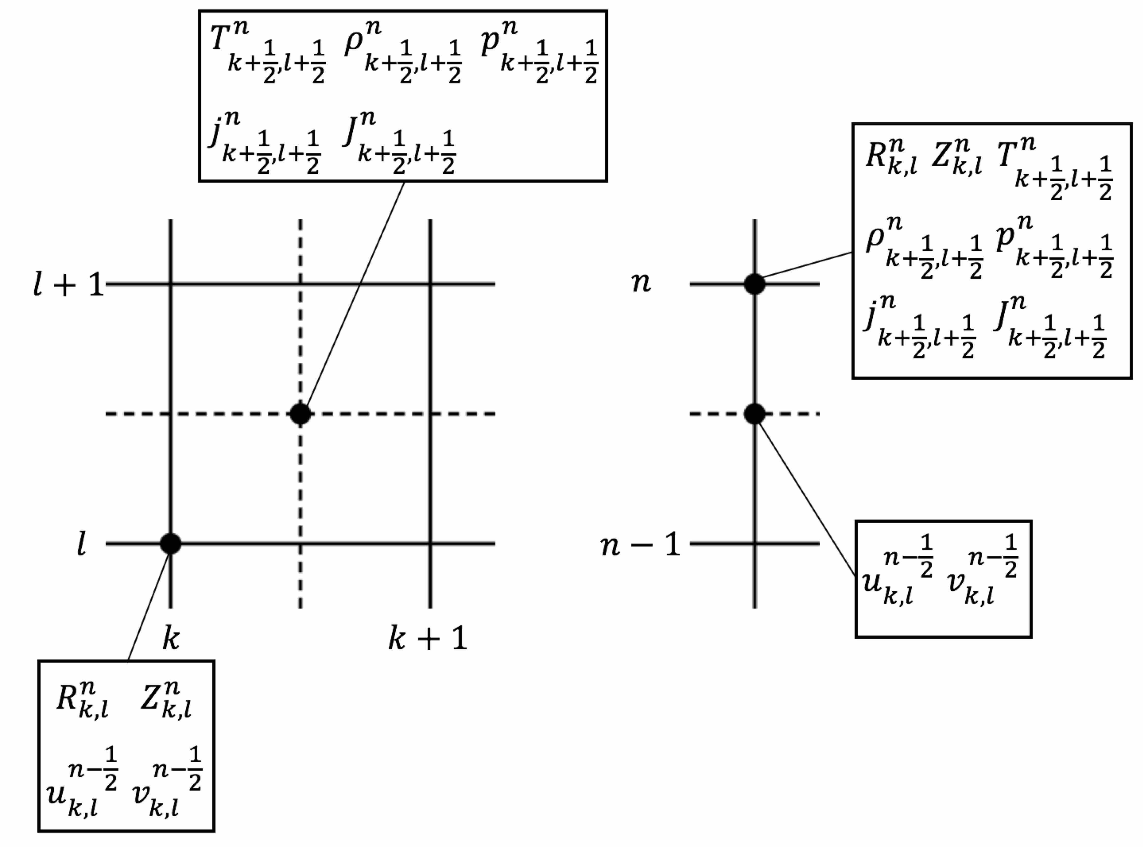
Figure 2: Definition points of discretized physical quantities in the Lagrangian code.

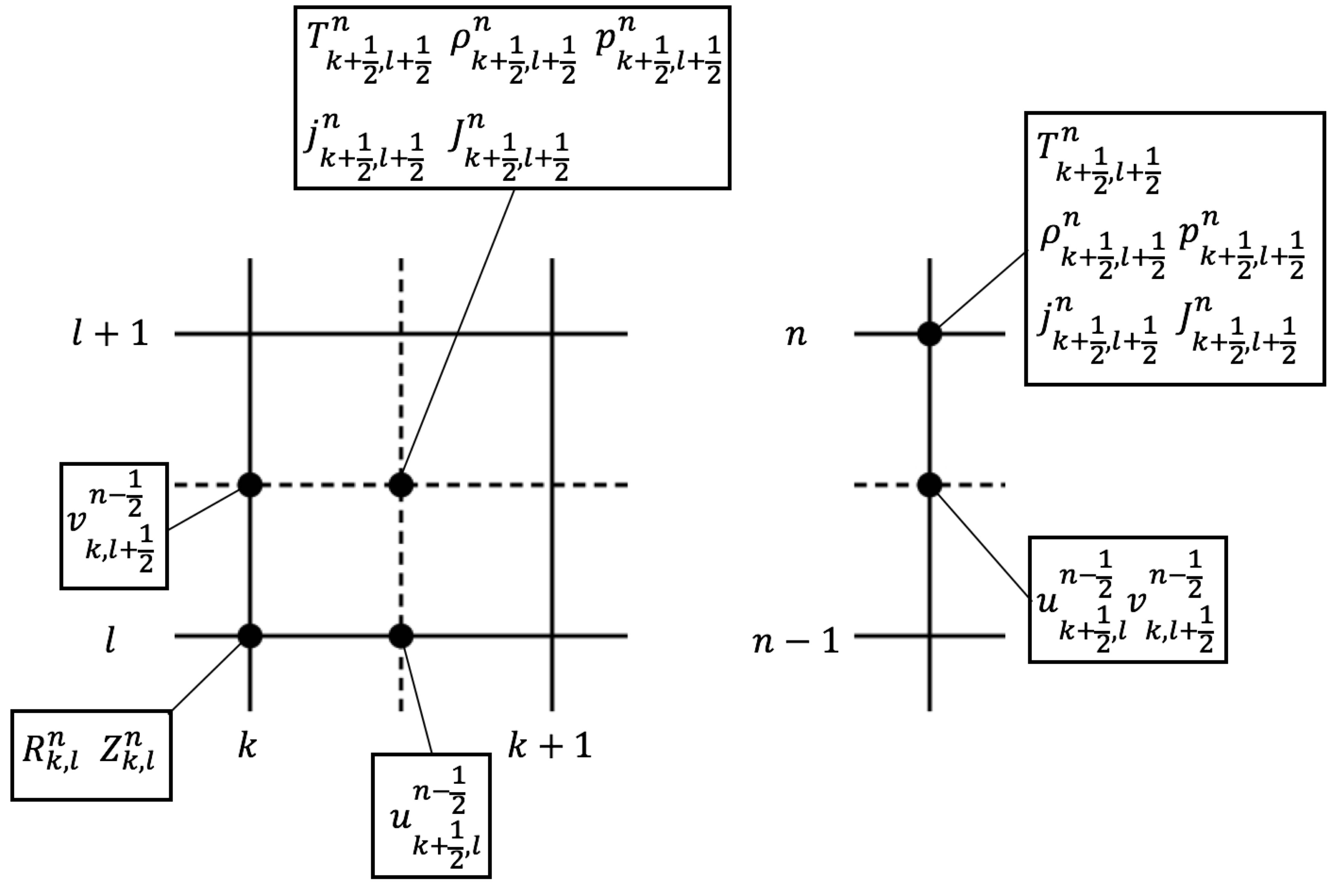
Figure 3: Definition points of discretized physical quantities in the Eulerian code.

3.1 Lagrangian code and OK3

1. BC_LC.cpp
   The boundary conditions are included in the procedure.

2. CONSTANT.h
   The file contains the definition of constant values and normalization factors.

3. Derf.c
   The file contains the error function in the double precision.

4. HIFScheme.h
   The file contains 1, 2, 3, 6, 12, 20, 32, 60 and 120-beam irradiation schemes. (see also Refs. [21, 22, 23].)

5. IMOK.cpp
   The file contains a procedure to transfer the data such as the target temperature and others to OK3. After the deposited energy distribution in OK3 is calculated, it is passed to the Lagrangian code.

6. InitMesh_LC.cpp
   The file initializes the Lagrangian coordinates and determines the number of the target layer. The number of the layers can be selected from 1 to 5 layers. The user must set the mesh number of each layer in this file.

7. InputOK3.h
   The input data file contains the target parameters, the HIB parameters, target mesh parameters and also the reactor chamber parameters.

8. Insulation.cpp
   The file contains a procedure to calculate the adiabat $\alpha$ with the following equations to evaluate the fuel preheating.

   $$\alpha = \frac{p}{\overline{p}}$$

   $$\overline{p} = p_{0}(\frac{\rho}{\rho_{0}})^{\frac{5}{3}}$$

   Here, $p$ and $\rho$ are the average pressure and mass density in the DT layer, respectively. $p_{0}$ and $\rho_{0}$ are the initial pressure and mass density in the DT layer, respectively.

9. Legendre.cpp
   The procedure performs the mode analyses based on the Legendre function in order to find the implosion non-uniformity. The analysis results are also output in this procedure.

10. Lr_LC.cpp
    A procedure to calculate the Rosseland mean free path (see Ref. [26]).

11. MS.cpp
    A function to solve matrix by the Gauss elimination method.

12. MS_TDMA.cpp
    A function to solve matrix by TDMA (TriDiagonal-Matrix Algorithm).

13. OK3code.cpp
    The file is the main routine of OK3 and contains the following procedures[21, 22, 23].
    Irradiation(): These procedures organizes a one-beam energy deposition process.
    InitEdp1(): This procedure calculates one-beamlet kinetic energy for each bunch. $E_{prt}$ is the energy of one projectile ion, $nE$ is a particle number parameter and $nBunch$ is the particle number in one bunch.
    Focus(): As shown in the Fig. 4, the position of the focal point must be determined. The procedure calculates the focal point distance $f$ as below :
    

    $$f=\frac{R_{\text{ch}}R_{\text{b}}-R_{\text{en}}R_{\text{p}}}{R_{\text{en}}-R_{\text{b}}}$$ (3)

    Here, $R_{b}$ is the beam radius on a tangential $\alpha$-plane, $R_{ch}$ the reactor chamber radius, $R_{p}$ the outer radius of the pellet and $R_{en}$ the beam radius on the chamber entrance.
    

    

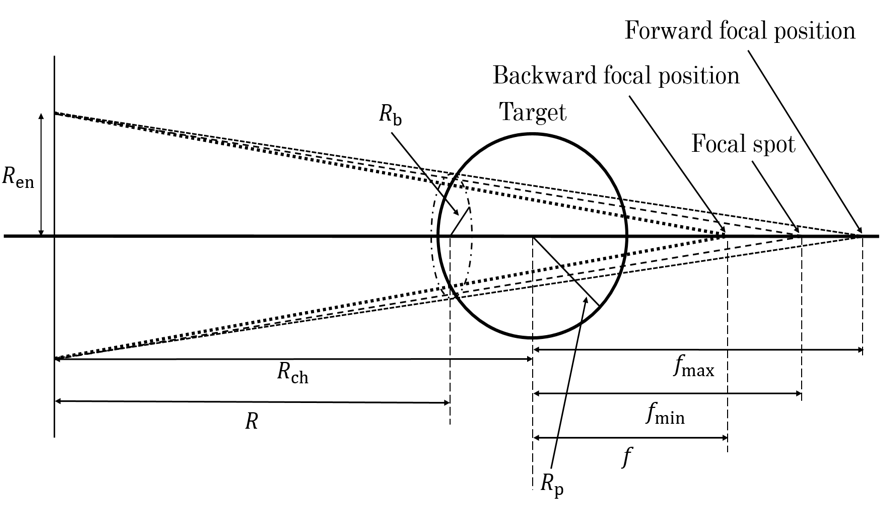
    Figure 4: Orbit of one beam to the target pellet

    fDis(): This procedure calculates the beam particle number density distribution coefficients $F_{ij}$.
    Divider(): This procedure organizes the beam division on beamlets. Each beamlet deposits its energy in the target independently.
    kBunch(): This procedure calculates the energy deposition coefficients $L_{ij}$ and $K_{ij}$ for each fixed mesh cell. $L_{ij}$ is the total trace length from one-particle traversal plane of each fixed beamlet, $d_{ij}$ the effective particle diameter and $K_{ij}$ the number of traversal planes for the beamlet.
    PointC(): Two spherical coordinate systems are used in the procedure as in Fig. 5, one linked to the reactor chamber center— Chamber System ($CS$) and another linked to the pellet center—Pellet System ($PS$). This procedure calculates the coordinates of the beam center on the pellet surface $r_{C}$ , $\theta_{C}$ and $\phi_{C}$ in $PS$.
    PointF(): This procedure calculates the coordinates of the focal point $f$: $r_{f}$ , $\theta_{f}$ and $\phi_{f}$ in $PS$.
    PointAlpha(): Each beamlet trajectory is fixed by two points in $PS$—the crossing point with a tangential $\alpha$-plane and the common focal point $F$ (see Fig. 5). This procedure calculates the coordinates $(r,\theta,\phi)$ to each $\alpha$-point in $PS$.
    

    

    Figure 5: The beamlets coordinate schemes[21].

    As mentioned in Section 1, there is an irradiation scheme called the spiral axis-oscillating wobbling HIBs, and a HIB irradiates the target pellet as shown in the Fig. 6. It is found that there is a smoothing effect for deposited energy deviation by rotating the beam axis. In OK 3, it is possible to calculate the HIBs energy deposition to the target pellet, when all beams wobble. The procedures related to the beam rotation are shown below.
    BeamCenterRot(): The procedure rotates the beam axis around the impinging direction of each beam.
    BeamletRot( ): The procedure rotates the beamlet axes that belong to each beam.
    Rotation(): The procedure sets the coordinates of rotated beams and beamlets in the reactor chamber and pellet systems.
    

    

    Figure 6: Conceptual diagram of spiral wobbling beam irradiating a fuel target

14. PelletSurface.h
    The file sets the initial target surface numerically.

15. RMS.cpp
    The procedure in this file calculates the root-mean-square (RMS) deviation in target non uniformity.

16. ResultIMP.cpp
    This file contains a procedure to calculate the implosion velocity.

17. SLC.cpp
    This file contains a procedure that outputs the time history of each physical quantities obtained by cutting out one of the theta directions.

18. StoppingPower1.cpp
    The file contains a function Stop1. This function serves a heart of the OK1 code [21] and describes the energy deposition model. It calculates the stopping power from the projectile ions into the solid target. The one-ion stopping power is considered to be a sum of the deposition energy in the target nuclei, the target bound and free electrons and the target ions[9].

19. Acceleration.cpp
    A procedure for calculating the target acceleration.

20. artv_LC.cpp
    This file contains a procedure calculate the artificial viscosity. When dealing with shock waves propagating in a compressive fluid at a supersonic speed in fluid dynamics simulations, it is impossible to employ sufficient number of multiple meshes to describe the real shock front structure, because its thickness is very thin. As a method, we introduce the following artificial viscosity devised by Von Neumann and Richtmyer[27].
    

    The two-dimensional artificial viscosity is written as follows[24]:

    $$q_{A}=-\rho c^{2}_{0}\left(\frac{\partial u}{\partial k}\right)^{A}_{\_}\left|\frac{\partial}{\partial k}\left(\frac{\partial u}{\partial k}\right)^{A}_{\_}\right|\\$$ (4)

    $$q_{B}=-\rho c^{2}_{0}\left(\frac{\partial u}{\partial l}\right)^{B}_{\_}\left|\frac{\partial}{\partial l}\left(\frac{\partial u}{\partial l}\right)^{B}_{\_}\right|$$ (5)

    $$\left(\frac{\partial u}{\partial k}\right)^{A}_{\_}=\min{\left[\left(\frac{\partial u}{\partial k}\right)^{A},0\right]}$$

    $$\left(\frac{\partial u}{\partial l}\right)^{B}_{\_}=\min{\left[\left(\frac{\partial u}{\partial l}\right)^{B},0\right]}$$

    $$\left(\frac{\partial u}{\partial k}\right)^{A}=\frac{\bar{\bm{R}}_{l}\cdot{\bm{u}}_{k}}{\left|\bar{\bm{R}}_{l}\right|}=\frac{Z_{l}u_{k}-R_{l}v_{k}}{\sqrt{Z^{2}_{l}+R^{2}_{l}}}$$

    $$\left(\frac{\partial u}{\partial l}\right)^{B}=\frac{\bar{\bm{R}}_{k}\cdot{\bm{u}}_{l}}{\left|\bar{\bm{R}}_{k}\right|}=\frac{Z_{k}u_{l}-R_{k}v_{l}}{\sqrt{Z^{2}_{k}+R^{2}_{k}}}$$

    Here, $q_{A}$ and $q_{B}$ are artificial viscosities for the directions of $\bar{\bm{R}}_{l}$ and $\bar{\bm{R}}_{k}$, respectively. Equations (4) and (5) are discretized and written as follows:

    $${q_{A}}^{n+\frac{1}{2}}_{k+\frac{1}{2},l+\frac{1}{2}}=\left({q_{A}1}^{n+\frac{1}{2}}_{k+\frac{1}{2},l+\frac{1}{2}}+{q_{A}3}^{n+\frac{1}{2}}_{k+\frac{1}{2},l+\frac{1}{2}}+{q_{A}1}^{n}_{k+\frac{1}{2},l+\frac{1}{2}}+{q_{A}3}^{n}_{k+\frac{1}{2},l+\frac{1}{2}}\right)$$ (6)

    $${q_{B}}^{n+\frac{1}{2}}_{k+\frac{1}{2},l+\frac{1}{2}}=\left({q_{B}2}^{n+\frac{1}{2}}_{k+\frac{1}{2},l+\frac{1}{2}}+{q_{B}4}^{n+\frac{1}{2}}_{k+\frac{1}{2},l+\frac{1}{2}}+{q_{B}2}^{n}_{k+\frac{1}{2},l+\frac{1}{2}}+{q_{B}4}^{n}_{k+\frac{1}{2},l+\frac{1}{2}}\right)$$ (7)

    Here,

    $${q_{A}1}^{n+1}_{k,l}=-c^{2}_{0}\rho^{n+\frac{1}{2}}_{k,l}dVa1_{k,l}ddVaf_{k,l}$$ (8)

    $${q_{B}2}^{n+1}_{k,l}=-c^{2}_{0}\rho^{n+\frac{1}{2}}_{k,l}dVb2_{k,l}ddVbf_{k,l}$$ (9)

    $${q_{A}3}^{n+1}_{k,l}=-c^{2}_{0}\rho^{n+\frac{1}{2}}_{k,l}dVa3_{k,l}ddVaf_{k,l}$$ (10)

    $${q_{B}4}^{n+1}_{k,l}=-c^{2}_{0}\rho^{n+\frac{1}{2}}_{k,l}dVb4_{k,l}ddVbf_{k,l}$$ (11)

    $$dVa_{k.l}=\min{\left[\frac{\delta\bar{\bm{R}}^{n}_{k+\frac{1}{2},l}\cdot\Delta{\bm{u}}^{n-\frac{1}{2}}_{k,l+\frac{1}{2}}}{\left|\delta\bar{\bm{R}}^{n}_{k+\frac{1}{2},l}\right|},\ 0\right]}$$

    $$dVb_{k.l}=\min{\left[-\frac{\Delta\bar{\bm{R}}^{n}_{k,l+\frac{1}{2}}\cdot\delta{\bm{u}}^{n-\frac{1}{2}}_{k+\frac{1}{2},l}}{\left|\Delta\bar{\bm{R}}^{n}_{k,l+\frac{1}{2}}\right|},\ 0\right]}$$

    $$ddVa_{k,l}=\left|dVa_{k+1,l}-dVa_{k,l}\right|$$

    $$ddVb_{k,l}=\left|dVb_{k,l+1}-dVb_{k,l}\right|$$

    $$ddVaf_{k.l}=\frac{1}{2}\{ddVa_{k,l}+ddVa_{k-1,l}\}$$

    $$ddVbf_{k,l}=\frac{1}{2}\{ddVb_{k,l}+ddVb_{k,l-1}\}.$$

21. coc_LC.cpp
    The file calculates the Lagrangian mesh dynamics. The Lagrangian meshes move together with the fluid motion. The new position coordinates for each mesh point are renewed at $n+1$.

22. cotc_define.h
    Define variables for calculating the heat conduction.

23. cotc_e.cpp, cotc_r.cpp
    For calculation of the heat conduction, the following basic equation is used[28].

    $$C_{V_{k}}\frac{DT}{Dt}=\frac{1}{\rho}{\bm{\nabla}}\cdot(\kappa_{k}{\bm{\nabla}}T_{k})\ \ \ \ \ \ \ (k=e,r)$$ (12)

    $$\ \ \ \ \kappa_{e}=1.83\times 10^{-10}T^{5/2}_{e}(\log{\Lambda})^{-1}Z^{-1}\ \ [{\rm W/mK}]$$

    $$\ \ \ \ \kappa_{r}=\frac{16}{3}\sigma L_{R}T^{3}_{r}\ \ [{\rm W/mK}]$$

    $$\kappa :Heatconductivity$$

    $$T_{k} :Ion,\ electron,\ radiation\ temperature[\rm K]$$

    $$\log{\Lambda} :Coulomb\ logarithm$$

    $$m :Mass$$

    $$Z :Ionization\ degree$$

    $$\sigma :Stefan-Boltzmann\ constant$$

    $$L_{R} :\rm{Rosseland\ mean\ free\ path}$$

    Here, the basic equation is transformed as follows:

    $$C_{V}\frac{DT}{Dt} = \frac{1}{\rho}{\bm{\nabla}}\cdot(\kappa{\bm{\nabla}}T)$$

    $$\int\!\!\!\!\int\!\!\!\!\int\rho C_{V}\frac{DT}{Dt}dV = \int\!\!\!\!\int\!\!\!\!\int{\rm\nabla}\cdot(\kappa{\bm{\nabla}}T)dV$$

    $$MC_{V}\frac{DT}{Dt} = \sum_{i}(\kappa{\bm{\nabla}}T)\cdot{\bm{S}_{i}}$$

    $$\frac{DT}{Dt} = \frac{1}{MC_{V}}\sum_{i}{\bm{S}_{i}}\cdot\bigg{[}\delta\bar{\bm{R}_{l}}\frac{\partial T}{\partial k}-\Delta\bar{\bm{R}_{k}}\frac{\partial T}{\partial l}\bigg{]}$$ (13)

    Equation (13) is discretized as follows:

    $$\begin{split}\frac{T^{n+1}_{k+\frac{1}{2},l+\frac{1}{2}}-T^{n}_{k+\frac{1}{2},l+\frac{1}{2}}}{dt^{n+\frac{1}{2}}}\!&=\!A_{1}\Bigl{(}T^{n+1}_{k+\frac{1}{2},l+\frac{1}{2}}\!-T^{n+1}_{k+\frac{1}{2},l-\frac{1}{2}}\Bigr{)}\!+\!A_{2}\Bigl{(}T^{n+1}_{k+\frac{1}{2},l+\frac{3}{2}}\!-T^{n+1}_{k+\frac{1}{2},l+\frac{1}{2}}\Bigr{)}\\ &+\!B_{1}\Bigl{(}T^{n+1}_{k+\frac{1}{2},l+\frac{1}{2}}\!-T^{n+1}_{k-\frac{1}{2},l+\frac{1}{2}}\Bigr{)}\!+\!B_{2}\Bigl{(}T^{n+1}_{k+\frac{3}{2},l+\frac{1}{2}}\!-T^{n+1}_{k+\frac{1}{2},l+\frac{1}{2}}\Bigr{)}\end{split}$$ (14)

    Here,

    $$A_{1}=-S^{n}_{k+\frac{1}{2},l}\bigg{|}\Delta\bar{\bm{R}}^{n}_{k+\frac{1}{2},l}\bigg{|}\frac{\kappa^{n}_{k+\frac{1}{2},l}}{j^{n}_{k+\frac{1}{2},l}}\ \ \ \ \ \ \ A_{2}=S^{n}_{k+\frac{1}{2},l+1}\bigg{|}\Delta\bar{\bm{R}}^{n}_{k+\frac{1}{2},l+1}\bigg{|}\frac{\kappa^{n}_{k+\frac{1}{2},l+1}}{j^{n}_{k+\frac{1}{2},l+1}}$$

    $$B_{1}=-S^{n}_{k,l+\frac{1}{2}}\bigg{|}\delta\bar{\bm{R}}^{n}_{k,l+\frac{1}{2}}\bigg{|}\frac{\kappa^{n}_{k,l+\frac{1}{2}}}{j^{n}_{k,l+\frac{1}{2}}}\ \ \ \ \ \ \ \ B_{2}=S^{n}_{k+1,l+\frac{1}{2}}\bigg{|}\delta\bar{\bm{R}}^{n}_{k+1,l+\frac{1}{2}}\bigg{|}\frac{\kappa^{n}_{k+1,l+\frac{1}{2}}}{j^{n}_{k+1,l+\frac{1}{2}}}.$$

24. define_LC.h
    It contains the procedure declarations for OK3 and the Lagrangian code.

25. dif_LC.cpp
    The following Lagrangian equation of motion is used[24].

    $$\rho\frac{D\bm{u}}{Dt}=-{\bm{\nabla}}p-\frac{\rho}{M}\left[\frac{\partial}{\partial k}(\hat{R}\bar{\bm{R}}_{l}q_{A})-\frac{\partial}{\partial l}(\hat{R}\bar{\bm{R}}_{k}q_{B})\right]$$ (15)

    Equation (15) is expressed for each component as follows:

    $$\rho\frac{Du}{Dt}=-\frac{\partial p}{\partial R}-\frac{\rho}{M}\left[\frac{\partial}{\partial k}(\hat{R}Z_{l}q_{A})-\frac{\partial}{\partial l}(\hat{R}Z_{k}q_{B})\right]$$ (16)

    $$\rho\frac{Dv}{Dt}=-\frac{\partial p}{\partial Z}-\frac{\rho}{M}\left[\frac{\partial}{\partial k}(\hat{R}(-R_{l})q_{A})-\frac{\partial}{\partial l}(\hat{R}(-R_{k})q_{B})\right]$$ (17)

    The above equations are converted to the Lagrangian differentiations, and the following equations are obtained.

    $$\frac{Du}{Dt}=-\frac{1}{\rho j}\left(Z_{l}\frac{\partial p}{\partial k}-Z_{k}\frac{\partial p}{\partial l}\right)-\frac{1}{M}\left[\frac{\partial}{\partial k}(\hat{R}Z_{l}q_{A})-\frac{\partial}{\partial l}(\hat{R}Z_{k}q_{B})\right]$$ (18)

    $$\frac{Dv}{Dt}=\frac{1}{\rho j}\left(R_{l}\frac{\partial p}{\partial k}-R_{k}\frac{\partial p}{\partial l}\right)-\frac{1}{M}\left[\frac{\partial}{\partial k}(\hat{R}R_{l}q_{A})-\frac{\partial}{\partial l}(\hat{R}R_{k}q_{B})\right]$$ (19)

    Equation (18) is discretized as follows:

    $$u^{n+\frac{1}{2}}_{k,l}=u^{n-\frac{1}{2}}_{k,l}-Dt^{n}\left[\left\{\frac{Z_{l}}{\rho j}\frac{\partial p}{\partial k}+\frac{1}{M}\frac{\partial}{\partial k}(\hat{R}Z_{l}q_{A}))\right\}^{n}_{k,l}-\left\{\frac{Z_{k}}{\rho j}\frac{\partial p}{\partial l}+\frac{1}{M}\frac{\partial}{\partial l}(\hat{R}Z_{k}q_{B}))\right\}^{n}_{k,l}\right]$$

    (20)

    Equation (20) is written as follows with the weight functions $\xi_{k,l},\eta_{k,l}$ and the artificial viscosities of $q_{A1},q_{A3},q_{B2}$ and $q_{B4}$.

    $$u^{n+\frac{1}{2}}_{k,l}=u^{n-\frac{1}{2}}_{k,l} - Dt^{n}[\eta_{k,l}TP_{1u}+(2-\eta_{k,l})TP_{3u}$$ (21)

    $$- \xi_{k.l}TP_{2u}-(2-\xi_{k,l})TP_{4u}]$$

    Here each symbol in Eq. (21) is listed below:

    $$\xi_{k,l}=\max{\left[0.2,\min{\{0.8,\xi^{\prime}_{k,l}\}}\right]}$$

    $$\eta_{k,l}=\max{\left[0.2,\min{\{0.8,\eta^{\prime}_{k,l}\}}\right]}$$

    $$\xi^{\prime}_{k.l}=\frac{2\omega_{k-\frac{1}{2},l}}{\omega_{k+\frac{1}{2},l}+\omega_{k-\frac{1}{2},l}},\ \eta^{\prime}_{k.l}=\frac{2\omega_{k,l-\frac{1}{2}}}{\omega_{k,l+\frac{1}{2}}+\omega_{k,l-\frac{1}{2}}}$$

    $$\omega_{k+\frac{1}{2},l}=\sqrt{\left(\frac{\Delta{\bm{R}}^{n}_{k+\frac{1}{2},l+\frac{1}{2}}+\Delta{\bm{R}}^{n}_{k+\frac{1}{2},l-\frac{1}{2}}}{2}\right)^{2}}$$

    $$\omega_{k,l\frac{1}{2}}=\sqrt{\left(\frac{\delta{\bm{R}}^{n}_{k+\frac{1}{2},l+\frac{1}{2}}+\delta{\bm{R}}^{n}_{k-\frac{1}{2},l+\frac{1}{2}}}{2}\right)^{2}}$$

    $$TP_{1u} = \frac{(Z_{l})^{n}_{k,l-\frac{1}{2}}\left(p^{n}_{k+\frac{1}{2},l-\frac{1}{2}}-p^{n}_{k-\frac{1}{2},l-\frac{1}{2}}\right)}{\rho^{n}_{k+\frac{1}{2},l-\frac{1}{2}}j^{n}_{k+\frac{1}{2},l-\frac{1}{2}}+\rho^{n}_{k-\frac{1}{2},l-\frac{1}{2}}j^{n}_{k-\frac{1}{2},l-\frac{1}{2}}}$$

    $$+ \frac{\hat{R}^{n}_{k+\frac{1}{2},l-\frac{1}{2}}{q_{A1}}^{n}_{k+\frac{1}{2},l-\frac{1}{2}}\left[(Z_{l})^{n}_{k+1,l-\frac{1}{2}}+(Z_{l})^{n}_{k,l-\frac{1}{2}}\right]}{2\left(M^{n}_{k+\frac{1}{2},l-\frac{1}{2}}+M^{n}_{k-\frac{1}{2},l-\frac{1}{2}}\right)}$$

    $$- \frac{\hat{R}^{n}_{k-\frac{1}{2},l-\frac{1}{2}}{q_{A1}}^{n}_{k-\frac{1}{2},l-\frac{1}{2}}\left[(Z_{l})^{n}_{k-1,l-\frac{1}{2}}+(Z_{l})^{n}_{k,l-\frac{1}{2}}\right]}{2\left(M^{n}_{k+\frac{1}{2},l-\frac{1}{2}}+M^{n}_{k-\frac{1}{2},l-\frac{1}{2}}\right)}$$

    $$TP_{2u} = \frac{(Z_{k})^{n}_{k-\frac{1}{2},l}\left(p^{n}_{k-\frac{1}{2},l+\frac{1}{2}}-p^{n}_{k-\frac{1}{2},l-\frac{1}{2}}\right)}{\rho^{n}_{k-\frac{1}{2},l+\frac{1}{2}}j^{n}_{k-\frac{1}{2},l+\frac{1}{2}}+\rho^{n}_{k-\frac{1}{2},l-\frac{1}{2}}j^{n}_{k-\frac{1}{2},l-\frac{1}{2}}}$$

    $$+ \frac{\hat{R}^{n}_{k-\frac{1}{2},l+\frac{1}{2}}{q_{B2}}^{n}_{k-\frac{1}{2},l+\frac{1}{2}}\left[(Z_{k})^{n}_{k-\frac{1}{2},l+1}+(Z_{k})^{n}_{k-\frac{1}{2},l}\right]}{2\left(M^{n}_{k-\frac{1}{2},l+\frac{1}{2}}+M^{n}_{k-\frac{1}{2},l-\frac{1}{2}}\right)}$$

    $$- \frac{\hat{R}^{n}_{k-\frac{1}{2},l-\frac{1}{2}}{q_{B2}}^{n}_{k-\frac{1}{2},l-\frac{1}{2}}\left[(Z_{k})^{n}_{k-\frac{1}{2},l-1}+(Z_{k})^{n}_{k-\frac{1}{2},l}\right]}{2\left(M^{n}_{k-\frac{1}{2},l+\frac{1}{2}}+M^{n}_{k-\frac{1}{2},l-\frac{1}{2}}\right)}$$

    $$TP_{3u} = \frac{(Z_{l})^{n}_{k,l+\frac{1}{2}}\left(p^{n}_{k+\frac{1}{2},l+\frac{1}{2}}-p^{n}_{k-\frac{1}{2},l+\frac{1}{2}}\right)}{\rho^{n}_{k+\frac{1}{2},l+\frac{1}{2}}j^{n}_{k+\frac{1}{2},l+\frac{1}{2}}+\rho^{n}_{k-\frac{1}{2},l+\frac{1}{2}}j^{n}_{k-\frac{1}{2},l+\frac{1}{2}}}$$

    $$+ \frac{\hat{R}^{n}_{k+\frac{1}{2},l+\frac{1}{2}}{q_{A3}}^{n}_{k+\frac{1}{2},l+\frac{1}{2}}\left[(Z_{l})^{n}_{k+1,l+\frac{1}{2}}+(Z_{l})^{n}_{k,l+\frac{1}{2}}\right]}{2\left(M^{n}_{k+\frac{1}{2},l+\frac{1}{2}}+M^{n}_{k-\frac{1}{2},l+\frac{1}{2}}\right)}$$

    $$- \frac{\hat{R}^{n}_{k-\frac{1}{2},l+\frac{1}{2}}{q_{A3}}^{n}_{k-\frac{1}{2},l+\frac{1}{2}}\left[(Z_{l})^{n}_{k-1,l+\frac{1}{2}}+(Z_{l})^{n}_{k,l+\frac{1}{2}}\right]}{2\left(M^{n}_{k+\frac{1}{2},l+\frac{1}{2}}+M^{n}_{k-\frac{1}{2},l+\frac{1}{2}}\right)}$$

    $$TP_{4u} = \frac{(Z_{k})^{n}_{k+\frac{1}{2},l}\left(p^{n}_{k+\frac{1}{2},l+\frac{1}{2}}-p^{n}_{k+\frac{1}{2},l-\frac{1}{2}}\right)}{\rho^{n}_{k+\frac{1}{2},l+\frac{1}{2}}j^{n}_{k+\frac{1}{2},l+\frac{1}{2}}+\rho^{n}_{k+\frac{1}{2},l-\frac{1}{2}}j^{n}_{k+\frac{1}{2},l-\frac{1}{2}}}$$

    $$+ \frac{\hat{R}^{n}_{k+\frac{1}{2},l+\frac{1}{2}}{q_{B2}}^{n}_{k+\frac{1}{2},l+\frac{1}{2}}\left[(Z_{k})^{n}_{k+\frac{1}{2},l+1}+(Z_{k})^{n}_{k+\frac{1}{2},l}\right]}{2\left(M^{n}_{k+\frac{1}{2},l+\frac{1}{2}}+M^{n}_{k+\frac{1}{2},l-\frac{1}{2}}\right)}$$

    $$- \frac{\hat{R}^{n}_{k+\frac{1}{2},l-\frac{1}{2}}{q_{B2}}^{n}_{k+\frac{1}{2},l-\frac{1}{2}}\left[(Z_{k})^{n}_{k+\frac{1}{2},l-1}+(Z_{k})^{n}_{k+\frac{1}{2},l}\right]}{2\left(M^{n}_{k+\frac{1}{2},l+\frac{1}{2}}+M^{n}_{k+\frac{1}{2},l-\frac{1}{2}}\right)}$$

26. dt_LC.cpp
    This procedure calculates and control the time step in order to satisfy the numerical stability condition. The time step $\Delta t$ in the calculation must satisfy the following conditions.

    $$\Delta t=\frac{\Delta r}{C_{S}+V_{max}}$$ (26)

    The time step for the Lagrangian method $Dt^{n+\frac{1}{2}}$ is represented by the following expression.

    $$Dt^{n+\frac{1}{2}}=\alpha\displaystyle\frac{dr_{min}}{C_{S}+V_{max}}$$ (27)

    	$\alpha$	: Numerical coefficient constant $(\alpha\leq 1)$
    	$dr_{min}$	: the minimum grid spacing
    	$C_{S}$	: Sound speed
    	$V_{max}$	: the maximum flow speed

27. eoenergy_LC.cpp
    The file contains a procedure for calculation of the energy equation and the HIBs input energy from OK3 code. The following Lagrangian equation of energy is used except for the heat conductions terms.

    $$\begin{cases}\frac{DT_{i}}{Dt}=-\frac{k_{B}}{C_{V_{i}}}\left[B_{T_{i}}\frac{D\rho}{Dt}+p_{i}\frac{D}{Dt}\left(\frac{1}{\rho}\right)+\frac{1}{\rho j}\{q_{A}(Z_{l}u_{k}-R_{l}v_{k})-q_{B}(Z_{k}u_{l}-R_{k}v_{l})\}\right]\\ \frac{DT_{e}}{Dt}=-\frac{k_{B}}{C_{V_{e}}}\left[B_{T_{e}}\frac{D\rho}{Dt}+p_{e}\frac{D}{Dt}\left(\frac{1}{\rho}\right)\right]\\ \frac{DT_{r}}{Dt}=-\frac{k_{B}}{C_{V_{r}}}\left[B_{T_{r}}\frac{D\rho}{Dt}+p_{r}\frac{D}{Dt}\left(\frac{1}{\rho}\right)\right]\end{cases}$$ (28)

    Equation (28) is discretized as follows:

    $$T^{n+1}_{k+\frac{1}{2},l+\frac{1}{2}} = T^{n}_{k+\frac{1}{2},l+\frac{1}{2}}$$

    $$- \frac{1}{{C_{V}}^{n+\frac{1}{2}}_{k+\frac{1}{2},l+\frac{1}{2}}}\Bigg{[}{B_{T}}^{n+1}_{k+\frac{1}{2},l+\frac{1}{2}}(\rho^{n+1}_{k+\frac{1}{2},l+\frac{1}{2}}-\rho^{n}_{k+\frac{1}{2},l+\frac{1}{2}})+p^{n+\frac{1}{2}}_{k+\frac{1}{2},l+\frac{1}{2}}(\tau^{n+1}_{k+\frac{1}{2},l+\frac{1}{2}}-\tau^{n}_{k+\frac{1}{2},l+\frac{1}{2}})$$

    $$+ \left.\frac{Dt^{n+\frac{1}{2}}\{{q_{A}}^{n+\frac{1}{2}}_{k+\frac{1}{2},l+\frac{1}{2}}(Z_{l}u_{k}-R_{l}v_{k})^{n+\frac{1}{2}}_{k+\frac{1}{2},l+\frac{1}{2}}-{q_{B}}^{n+\frac{1}{2}}_{k+\frac{1}{2},l+\frac{1}{2}}(Z_{k}u_{l}-R_{k}v_{l})^{n+\frac{1}{2}}_{k+\frac{1}{2},l+\frac{1}{2}}\}}{\rho^{n+\frac{1}{2}}_{k+\frac{1}{2},l+\frac{1}{2}}j^{n+\frac{1}{2}}_{k+\frac{1}{2},l+\frac{1}{2}}}\right]$$

28. eos.cpp
    The file contains the procedures to calculate the following equation of state. The equations of state for ions and various physical quantities are shown below:

    $$\begin{cases}P_{i}=n_{i}k_{B}T_{i}\\ U_{i}=\frac{3}{2}\frac{k_{B}T_{i}}{m_{p}M}\\ C_{vi}=\Bigl{(}\frac{\partial U_{i}}{\partial T_{i}}\Bigr{)}_{v}=\frac{3}{2}\frac{k_{B}}{m_{p}M}\end{cases}$$ (29)

    	$P_{i}$	: Ion pressure$[{\rm Pa}]$
    	$n_{i}$	: Ion number density$[{\rm 1/m^{3}}]$
    	$T_{i}$	: Ion temperature$[{\rm eV}]$
    	$U_{i}$	: Ion specific energy$[{\rm J/kg}]$
    	$C_{vi}$	: Ion specific heat at constant volume$[{\rm J/K}\cdot{\rm kg}]$
    	$m_{p}$	: Mass of proton$[{\rm kg}]$
    	$k_{B}$	: Boltzmann constant$[{\rm J/K}]$
    	$M$	: Atomic weight

    For the equation of state for electrons, we use the equation of state based on the Thomas-Fermi model shown in Ref. [29]. Users can select the Thomas-Fermi model or the ideal equation of state in the header file of ”input_LC.h”.
    

    For the equation of state for the radiation, we use the following equations:
    

    Radiation energy ${\bm{U}_{r}}$

    $$U_{r}=\frac{4\sigma T^{4}_{r}}{\rho c}$$ (30)

    Radiation pressure ${\bm{P}_{r}}$

    $$P_{r}=\frac{4}{3}\frac{\sigma T^{4}_{r}}{c}$$ (31)

    Radiation specific heat at constant volume ${\bm{C}_{V_{r}}}$

    $$C_{V_{r}}=\frac{16\sigma T^{3}_{4}}{\rho c}$$ (32)

    Here, various physical quantities are shown below.

    	$k_{B}$	: Boltzmann constant
    	$T_{I,e,r}$	: Temperature
    	$\rho$	: Mass density
    	$j,J$	: Area and volume per mesh
    	$M$	: Mass
    	$n$	: Number density
    	$p_{i,e,r}$	: Pressure
    	$C_{V_{i,e,r}}$	: Specific heat at the constant volume
    	$B_{T_{i,e,r}}$	: Compressibility
    	$q_{A},q_{B}$	: Artificial viscosity
    	$\sigma$	: Stefan-Boltzmann constant
    	$c$	: Speed of light

29. init_LC.h
    It contains the initial conditions such as the energy driver projectile, the initial target temperature and so on.

30. input_LC.h
    The input data for Lagrangian code contains the target layer thickness, the input beam pulse, the beam radius and so on.

31. jacobian_LC.cpp
    The area and volume per mesh are calculated in this file. Jacobian $j$ for the coordinate transformation from $(R,\ Z)$ to $(k,\ l)$ is expressed by the following formula. $j$ represents the area of the mesh.

    $$j=\frac{\partial R}{\partial k}\frac{\partial Z}{\partial l}-\frac{\partial R}{\partial l}\frac{\partial Z}{\partial k}=R_{k}Z_{l}-R_{l}Z_{k}$$ (33)

    The volume Jacobian is as follows.

    $$J=Rj$$ (34)

    From Eq. (33), the area Jacobian is expressed as follows:

    $$j^{n}_{k+\frac{1}{2},l+\frac{1}{2}}=\Bigl{(}\frac{\partial R}{\partial k}\Bigr{)}^{n}_{k+\frac{1}{2},l+\frac{1}{2}}\Bigl{(}\frac{\partial Z}{\partial l}\Bigr{)}^{n}_{k+\frac{1}{2},l+\frac{1}{2}}-\Bigl{(}\frac{\partial R}{\partial l}\Bigr{)}^{n}_{k+\frac{1}{2},l+\frac{1}{2}}\Bigl{(}\frac{\partial Z}{\partial k}\Bigr{)}^{n}_{k+\frac{1}{2},l+\frac{1}{2}}$$ (35)

    Here,

    $$\Bigl{(}\frac{\partial R}{\partial k}\Bigr{)}^{n}_{k+\frac{1}{2},l+\frac{1}{2}}=\frac{\Delta R^{n}_{k+\frac{1}{2},l+1}+\Delta R^{n}_{k+\frac{1}{2},l}}{2}$$

    $$\Bigl{(}\frac{\partial R}{\partial l}\Bigr{)}^{n}_{k+\frac{1}{2},l+\frac{1}{2}}=\frac{\delta R^{n}_{k+1,l+\frac{1}{2}}+\delta R^{n}_{k,l+\frac{1}{2}}}{2}$$

    $$\Bigl{(}\frac{\partial Z}{\partial k}\Bigr{)}^{n}_{k+\frac{1}{2},l+\frac{1}{2}}=\frac{\Delta Z^{n}_{k+\frac{1}{2},l+1}+\Delta Z^{n}_{k+\frac{1}{2},l}}{2}$$

    $$\Bigl{(}\frac{\partial Z}{\partial l}\Bigr{)}^{n}_{k+\frac{1}{2},l+\frac{1}{2}}=\frac{\delta Z^{n}_{k+1,l+\frac{1}{2}}+\delta Z^{n}_{k,l+\frac{1}{2}}}{2}.$$

    Therefore,

    $$j^{n}_{k+\frac{1}{2},l+\frac{1}{2}} = \frac{\Delta R^{n}_{k+\frac{1}{2},l+1}+\delta R^{n}_{k+\frac{1}{2},l}}{2}\frac{\delta Z^{n}_{k+1,l+\frac{1}{2}}+\delta Z^{n}_{k,l+\frac{1}{2}}}{2}$$ (36)

    $$- \frac{\delta R^{n}_{k+1,l+\frac{1}{2}}+\delta R^{n}_{k,l+\frac{1}{2}}}{2}\frac{\Delta Z^{n}_{k+\frac{1}{2},l+1}+\Delta Z^{n}_{k+\frac{1}{2},l}}{2}$$

    $$= \frac{1}{4}\left[\left(\Delta R^{n}_{k+\frac{1}{2},l+1}+\Delta R^{n}_{k+\frac{1}{2},l}\right)\left(\delta Z^{n}_{k+1,l+\frac{1}{2}}+\delta Z^{n}_{k,l+\frac{1}{2}}\right)\right.$$

    $$- \left.\left(\delta R^{n}_{k+1,l+\frac{1}{2}}+\delta R^{n}_{k,l+\frac{1}{2}}\right)\left(\Delta Z^{n}_{k+\frac{1}{2},l+1}+\Delta Z^{n}_{k+\frac{1}{2},l}\right)\right].$$

    The discretization of volume Jacobian $J$ is as follows:

    $$J^{n}_{k+\frac{1}{2},l+\frac{1}{2}} = \frac{1}{6}\left({\hat{R}}^{n}_{k,l}+{\hat{R}}^{n}_{k,l+1}+{\hat{R}}^{n}_{k+1,l}\right)\cdot\left(\Delta R^{n}_{k+\frac{1}{2},l}\delta Z^{n}_{k,l+\frac{1}{2}}-\Delta Z^{n}_{k+\frac{1}{2},l}\delta R^{n}_{k,l+\frac{1}{2}}\right)$$

    $$+ \frac{1}{6}\left({\hat{R}}^{n}_{k+1,l+1}+{\hat{R}}^{n}_{k,l+1}+{\hat{R}}^{n}_{k+1,l}\right)\cdot$$

    $$\left(\Delta R^{n}_{k+\frac{1}{2},l+1}\delta Z^{n}_{k+1,l+\frac{1}{2}}-\Delta Z^{n}_{k+\frac{1}{2},l+1}\delta R^{n}_{k+1,l+\frac{1}{2}}\right)$$

32. main_LC.cpp
    The main procedure of the Lagrangian fluid code.

33. outputRMS.cpp
    It contains a procedure to output the results for the RMS non-uniformity.

34. output_LC.cpp
    The result data are stored by this procedure. The time interval of data output is 0.01 ns in the Lagrangian code. The user can adjust the output step in ”input_LC.h”.

35. output_to_EulerCode.cpp
    This file contains a procedure for outputting the data used in Euler code. The data is output, when the position of the innermost mesh is 1.5 mm or less from the coordinate center.

36. relax.cpp
    The following equation is used as the basic equation for the temperature relaxation[25].

    $$\begin{cases}C_{V_{i}}\frac{dT_{i}}{dt}=-K_{ie}\\ C_{V_{e}}\frac{dT_{e}}{dt}=K_{ie}-K_{re}\\ C_{V_{r}}\frac{dT_{r}}{dt}=K_{re}\end{cases}$$ (38)

    Here, $K_{ie}$ is the energy exchange rate between the ions and the electrons, $K_{re}$ the energy exchange rate between the radiation and the electrons.

    $$\begin{cases}K_{ie}=C_{V_{i}}\omega_{ie}(T_{i}-T_{e})\\ K_{re}=C_{V_{r}}\omega_{re}(T_{e}-T_{r})\end{cases}$$ (39)

    $\omega_{ie}and\ \omega_{re}$ are the collision frequencies between the ions and the electrons and between the radiation and the electrons, respectively. They are obtained by the following formulae: The Compton effect between the radiation and the electrons is included.

    $$\omega_{ie}=\frac{Z^{2}e^{4}n\log{\Lambda}\sqrt{m_{e}}}{32\sqrt{2}\pi\varepsilon^{2}_{0}Mm_{p}(kT)^{3/2}}\ [\rm 1/s]$$ (40)

    $$\omega_{re}=\omega^{\prime}_{re}+\omega_{cr}$$

    $$\ \ \ \omega^{\prime}_{re}=8.5\times 10^{-14}\frac{\langle Z^{2}\rangle\langle Z\rangle n_{i}Ig}{MT^{1/2}_{e}c_{e}}\ [{\rm 1/s}]$$ (41)

    $$\ \ \ \ \ Ig=\int^{\infty}_{0}\frac{\xi(e^{\xi u}-e^{u})}{(\xi-1)(e^{\xi u}-1)(e^{u}-1)}du$$

    $$\ \ \ \omega_{cr}=\frac{128}{3}\frac{\pi e^{4}\sigma}{(m_{e}c^{2})^{3}}T^{4}_{r}=7.362\times 10^{-22}T^{4}_{r}\ [{\rm 1/s}]$$ (42)

    Here, $u=\displaystyle\frac{h\ mu}{kT_{e}},\ \xi=\displaystyle\frac{T_{e}}{T_{i}}$ and $h$ is Planck’s constant, $\mu$ the collision frequency.

    $$\begin{cases}C^{n+\frac{1}{2}}_{V_{i}}\displaystyle\frac{T^{n+1}_{i}-T^{*}_{i}}{\Delta t^{n+\frac{1}{2}}}=-K^{n+\frac{1}{2}}_{ie}\\[10.0pt] C^{n+\frac{1}{2}}_{V_{e}}\displaystyle\frac{T^{n+1}_{e}-T^{*}_{e}}{\Delta t^{n+\frac{1}{2}}}=K^{n+\frac{1}{2}}_{ie}-K^{n+\frac{1}{2}}_{re}\\[10.0pt] C^{n+\frac{1}{2}}_{V_{r}}\displaystyle\frac{T^{n+1}_{r}-T^{*}_{r}}{\Delta t^{n+\frac{1}{2}}}=-K^{n+\frac{1}{2}}_{re}\\ \end{cases}$$ (43)

    $T^{*}$ represents the temperature after calculation with the energy equation. Discretizing the energy exchange rates are written as follows with $\xi_{ie}=T_{i}-T_{e}$ and $\xi_{re}=T_{e}-T_{r}$.

    $$\begin{cases}K^{n+\frac{1}{2}}_{ie}=C_{V_{i}}\omega^{n+\frac{1}{2}}_{ie}\xi^{n+\frac{1}{2}}_{ie}\\ K^{n+\frac{1}{2}}_{re}=C_{V_{r}}\omega^{n+\frac{1}{2}}_{re}\xi^{n+\frac{1}{2}}_{re}\end{cases}$$ (44)

    $\xi^{n+\frac{1}{2}}_{ie}$ and $\xi^{n+\frac{1}{2}}_{re}$ are as follows.

    $$\xi^{n+\frac{1}{2}}_{ie}=C_{i}A+\bigg{[}\xi^{n}_{ie}-\Bigl{(}\frac{\alpha_{i}}{\gamma}\Bigr{)}^{n+\frac{1}{2}}\bigg{]}B+\Bigl{(}\frac{\alpha_{i}}{\gamma}\Bigr{)}^{n+\frac{1}{2}}$$

    $$\xi^{n+\frac{1}{2}}_{re}=C_{r}A+\bigg{[}\xi^{n}_{re}-\Bigl{(}\frac{\alpha_{r}}{\gamma}\Bigr{)}^{n+\frac{1}{2}}\bigg{]}B+\Bigl{(}\frac{\alpha_{r}}{\gamma}\Bigr{)}^{n+\frac{1}{2}}$$

    The variables in the formulae are represented below.

    $$\alpha_{i}=(\phi_{i}+\beta_{r}\phi_{r})\omega_{re},\quad\alpha_{r}=(\phi_{i}G+\beta_{i}\phi_{r})\omega_{ie}$$

    $$\beta_{i}=1+\frac{C_{V_{i}}}{C_{V_{e}}},\quad\beta_{r}=1+\frac{C_{V_{e}}}{C_{V_{r}}},\quad G=\frac{C_{V_{i}}}{C_{V_{e}}},\quad\gamma=(\beta_{i}\beta_{r}-G)\omega_{ie}\omega_{re}$$

    $$A=\frac{\bigg{[}\exp{\Bigl{(}X\Delta t^{n+\frac{1}{2}}\Bigr{)}}-1\bigg{]}}{X\Delta t^{n+\frac{1}{2}}}-\frac{\bigg{[}\exp{\Bigl{(}Y\Delta t^{n+\frac{1}{2}}\Bigr{)}}-1\bigg{]}}{Y\Delta t^{n+\frac{1}{2}}}$$

    $$B=\frac{\bigg{[}\exp{\Bigl{(}Y\Delta t^{n+\frac{1}{2}}\Bigr{)}}-1\bigg{]}}{Y\Delta t^{n+\frac{1}{2}}}$$

    $$X=-\frac{1}{2}\lambda+\frac{1}{2}(\lambda^{2}-4\gamma)^{n+\frac{1}{2}},\quad Y=-\frac{1}{2}\lambda-\frac{1}{2}(\lambda^{2}-4\gamma)^{n+\frac{1}{2}}$$

    $$C_{i}=\frac{1}{(\lambda^{2}-4\gamma)^{n+\frac{1}{2}}}\bigg{[}\phi_{i}-\beta_{i}\omega_{ie}\xi_{i0}+\omega_{re}\xi_{r0}+\frac{1}{2}\lambda\Bigl{(}\xi_{i0}-\frac{\alpha_{i}}{\gamma}\Bigr{)}\bigg{]}$$

    $$+\frac{1}{2}\lambda\Bigl{(}\xi_{i0}-\frac{\alpha_{i}}{\gamma}\Bigr{)}$$

    $$C_{r}=\frac{1}{(\lambda^{2}-4\gamma)^{n+\frac{1}{2}}}\bigg{[}\phi_{r}-\beta_{r}\omega_{re}\xi_{r0}+G\omega_{ie}\xi_{i0}+\frac{1}{2}\lambda\Bigl{(}\xi_{r0}-\frac{\alpha_{r}}{\gamma}\Bigr{)}\bigg{]}$$

    $$+\frac{1}{2}\lambda\Bigl{(}\xi_{r0}-\frac{\alpha_{r}}{\gamma}\Bigr{)}$$

    $$\lambda=\beta_{i}\omega_{ie}+\beta_{r}\omega_{re},\quad\phi_{i}=\frac{W_{i}}{C_{V_{i}}}-\frac{W_{e}}{C_{V_{e}}},\quad\phi_{r}=\frac{W_{e}}{C_{V_{e}}}-\frac{W_{r}}{C_{V_{r}}}$$

37. relax_define.h
    It contains the procedure declarations for the temperature relaxation.

3.2 Conversion code

1. Check_EuMesh.sh This shell creates symbolic links connecting to the output files from the Lagrangian code. The shell file must have an execution permission. When the O-SUKI code is run on your computer by using the ”O-SUKIcode_start.sh”, the ”O-SUKIcode_start.sh” changes the permission of the ”Check_EuMesh.sh” to executable.

2. Check_CP.sh This shell retrieves the file name of the linked data file from the Lagrangian code. For example, when the link name has the name of ’EuCopy0001.dat’ and the original data file name may be ’Euler_n_00080754_t_2.750010e+01.dat’, the following command returns the original data file name.
   
   $ Check_CP.sh 0001
   $ lrwxrwxrwx $\cdot\cdot\cdot$ EuCopy0001.dat $\to$ Euler_n_00080754_t_2.750010e+01.dat
   

   The shell is used, when users need to know the linked file name.

3. check_quantities.cpp The function outputs the data of the transformed Euler mesh as a text file.

4. define_convert.h Define the variables necessary for the conversion code.

5. DownConvert.cpp The procedure to compress four Eulerian meshes into one mesh. The process is the down-conversion program. Initially the computing spatial area in the $R$ and $Z$ directions is specified in ”main_convert.cpp”. The minimum mesh size is determined in ”GenerateEulerMesh.cpp”. The minimum mesh size is equal to the minimum mesh size of the Lagrangian mesh size. The Euler mesh shape is a foursquare. It may be necessary to reduce the mesh number so that it does not exceed 300 which is the maximum allowable mesh $k$ number in the Euler code in one coordinate direction. The physical quantity definition points are shown in the Fig.7 during the down-conversion process. To perform the down conversion, the mesh number must be an even number so that this process is executed multiple times. For example, the relation of the number ($km$) of meshes in the $k$ direction before and after the down-convert is shown below as the number $p$ of the down-convert processing.

   $$km_{before}=2^{p}km_{after}+2$$ (45)

   The down conversion can be performed by $p$ times in this case. As the down-conversion time increases, the calculation results will be affected. In O-SUKI, the number of the down conversion is limited to 4 times. Therefore, the maximum allowable number of the Euler meshes before the conversion ($km_{before}$) is about 4800. If $km_{before}$ is larger than 4800, the down conversion limit number 4 should be set to a larger number in ”define_convert.h”.

   

   Figure 7: Definition points of each physical quantity and the down-convert

6. GenerateEulerMesh.cpp The procedure to determine the number of the Euler meshes and to secure the necessary memory, just before the down conversion.

7. GenerateEulerMesh_numSearch.cpp The procedure to check the number of the Euler meshes based on the minimum mesh size obtained in ”main_convert.cpp”. The procedure is similar to the procedure of ”GenerateEulerMesh.cpp”, but it is used during the selection of the data conversion dataset at a specific time.

8. Interpolation.cpp The function interpolates the data on the Lagrangian mesh to the meshes on the Euler mesh. Figure 8 shows the interpolation method from the Lagrange data to the Euler data. The ”MeshSearch.cpp” provides the relation between the Lagrangian mesh location and the Euler mesh location. The following interpolation equation is used to obtain each physical quantity on the Euler meshes. Here $x$ shows an arbitrary physical quantity.

   $$\begin{split}x(P)&=\frac{1}{\left(\displaystyle\frac{1}{|\overrightarrow{dist_{k,l}}|}\right)^{2}+\left(\displaystyle\frac{1}{|\overrightarrow{dist_{k+1,l}}|}\right)^{2}+\left(\displaystyle\frac{1}{|\overrightarrow{dist_{k,l+1}}|}\right)^{2}+\left(\displaystyle\frac{1}{|\overrightarrow{dist_{k+1,l+1}}|}\right)^{2}}\\[13.0pt] &\times\left(\!\frac{1}{|\overrightarrow{dist_{k,l}}|}x_{k,l}\!+\frac{1}{|\overrightarrow{dist_{k+1,l}}|}x_{k+1,l}\!+\frac{1}{|\overrightarrow{dist_{k,l+1}}|}x_{k,l+1}\!+\frac{1}{|\overrightarrow{dist_{k+1,l+1}}|}x_{k+1,l+1}\!\right)\end{split}$$ (46)

   

   Figure 8: The interpolation of physical quantity

9. main_convert.cpp This is the main procedure of the conversion code. This procedure selects the output Lagrangian data transferred to the Euler code among the Lagrangian data sets obtained in the Lagrangian code. The Lagrangian meshes are deformed along with the fluid motion. The Lagrangian code stops before no mesh is crushed. The data selection process is as follows:
   
   

   1. From the Lagrangian data at a specific time, the square area covered by the position of the maximum ion temperature and the origin is selected, and is simulated in the Euler code. The minimum mesh size is detected from the Lagrangian data. The uniform Euler mesh size is set to the minimum mesh size in the Lagrangian data. The Euler total mesh number required is determined to cover the selected area.
      

   2. The procedure selects the Lagrangian data, which needs the smallest number of the total Euler mesh among the data sets for the final 1.5 ns in the Lagrangian code. If the total mesh number $km$ in the $k$ direction exceeds 300, the data down conversion takes place to reduce $km$, which should be less than 300 in the O-SUKI code.
      

   3. The default maximum down conversion number is limited to 4. In this prescription, the maximum Euler mesh number is 4800 in the $k$ direction. If the selected data from the Lagrangian data set has the meshes more than 4800, first the square area selected in the Step 1 is reduced to fulfill the mesh number requirement of 4800. The area reduction is performed by reducing the size in the $k$ direction by 0.01 mm. The reduction procedure is repeated until the total mesh number becomes less than 4800 in the $k$ direction.
      

   4. If the total number of the Euler meshes exceeds 4800, the limit number of down conversion, which is specified in ”define_convert.h”, should be set to a larger number manually. However, many down conversion operations do not guarantee the numerical accuracy.
      

10. MeshSearch.cpp This procedure examines the location of each Euler mesh among the Lagrangian meshes. In Fig. 8, $\vec{P}$ represents the coordinate vector of a specific Euler mesh and $\vec{R}$ represents the coordinate vector of the Lagrangian mesh. The $\vec{V}_{1}$, $\vec{V}_{2}$, $\vec{V}_{3}$, $\vec{V}_{1}P$, $\vec{V}_{2}P$ and $\vec{V}_{3}P$ in Fig. 8 are indicated by the vectors of the Lagrangian meshes and the Euler mesh as follows:

    $$\begin{cases}{\vec{V}}_{1}={\vec{R}}_{k,l}-{\vec{R}}_{k+1,l}\\ {\vec{V}}_{2}={\vec{R}}_{k+1,l+1}-{\vec{R}}_{k,l}\\ {\vec{V}}_{3}={\vec{R}}_{k+1,l}-{\vec{R}}_{k+1,l+1}\end{cases}\begin{cases}\overrightarrow{V_{1}P}={\vec{P}}-{\vec{R}}_{k+1,l}\\ \overrightarrow{V_{2}P}={\vec{P}}-{\vec{R}}_{k,l}\\ \overrightarrow{V_{3}P}={\vec{P}}-{\vec{R}}_{k+1,l+1}\end{cases}$$

    If the cross product of each side vector of the triangle and the point P satisfies the following condition, the point P exists inside the triangle.

    $$\begin{cases}{\vec{V}}_{1}\times\overrightarrow{V_{1}P}<0\\ {\vec{V}}_{2}\times\overrightarrow{V_{2}P}<0\\ {\vec{V}}_{3}\times\overrightarrow{V_{3}P}<0\end{cases}$$ (47)

11. output.cpp In this procedure the converted data is output.

12. read_variable.cpp This procedure reads the file data output by the Lagrange code, after the Lagrangian data set selection.

13. read_variable_numSearch.cpp This procedure reads the data by the Lagrangian code during the Lagrangian data set selection in the procedure of the ”main_convert.cpp”.

3.3 Eulerian code

1. BoundaryTracking.cpp
   It is a function to track the material boundary lines. Each boundary point is specified by the coordinates of the two variables: $BoundaryMesh\_k$ and $BoundaryMesh\_l$. The function interpolates the velocities $u$ and $v$ at the coordinates by the area interpolation, and tracks the positions of each boundary point. In Fig. 9 dotted lines represent the material boundaries. When the boundary point exists at the position shown in Fig. 10, the boundary point velocity ($u_{b},\ v_{b}$) is calculated by the area interpolation method and can be obtained by the following equations:

   $$u_{b} = S_{u1}u_{k,l+1}+S_{u2}u_{k,l}+S_{u3}u_{k+1,l+1}+S_{u4}u_{k+1,l}$$ (48)

   $$v_{b} = S_{v1}v_{k,l+1}+S_{v2}v_{k,l}+S_{v3}v_{k+1,l+1}+S_{v4}v_{k+1,l}$$ (49)

   

   Figure 9: Material boundary points.

   

   Figure 10: Velocity interpolation by the area interpolation.

2. GenerateMatrix.cpp
   The mesh total numbers of $(km,\ lm)$ are loaded from the converted data in GenerateMatrix(). all the variables required in the Euler code are defined based on the number $(km,\ lm)$.

3. Legendre.cpp
   The procedure performs the mode analyses based on the Legendre function in order to find the implosion non-uniformity. The analysis results are also output in this procedure.

4. MS_TDMA.cpp
   It is a function to solve matrix by TDMA (TriDiagonal-Matrix Algorithm).

5. MaterialDiscrimination.cpp
   It is a function to discriminate each material by the material boundary lines.

6. PaintMaterial.cpp
   The material is specified between the two material boundary lines in the procedure.

7. RMFP_ECSH.cpp
   It is a procedure to calculate the Rosseland mean free path (see Ref. [26]).

8. ScanLine.cpp
   It is a procedure that specifies the material on each Euler mesh.

9. artv_ECSH.cpp
   This file contains a procedure to calculate the artificial viscosity. The two-dimensional artificial viscosity is written as follows:

   $$q_{r}=\rho C_{Q}\left(\frac{\partial u}{\partial k}\right)^{2}+\rho C_{L}c_{0}\left|\frac{\partial u}{\partial k}\right|$$ (50)

   $$q_{z}=\rho C_{Q}\left(\frac{\partial v}{\partial l}\right)^{2}+\rho C_{L}c_{0}\left|\frac{\partial v}{\partial l}\right|$$ (51)

   Here, the discretized artificial viscosity is shown below:

   $${q_{r}}^{n}_{k+\frac{1}{2},l+\frac{1}{2}}\!\! = \!\rho^{n}_{k+\frac{1}{2},l+\frac{1}{2}}C_{Q}\!\left(u^{n}_{k+1,l+\frac{1}{2}}\!-u^{n}_{k,l+\frac{1}{2}}\right)^{2}\!\!\!$$ (52)

   $$+ \!\rho^{n}_{k+\frac{1}{2},l+\frac{1}{2}}C_{L}c_{0}\!\left|u^{n}_{k+1,l+\frac{1}{2}}\!-u^{n}_{k,l+\frac{1}{2}}\right|$$

   $${q_{z}}^{n}_{k+\frac{1}{2},l+\frac{1}{2}}\!\! = \!\rho^{n}_{k+\frac{1}{2},l+\frac{1}{2}}C_{Q}\!\left(v^{n}_{k+\frac{1}{2},l+1}-v^{n}_{k+\frac{1}{2},l}\right)^{2}\!\!\!$$ (53)

   $$+ \!\rho^{n}_{k+\frac{1}{2},l+\frac{1}{2}}C_{L}c_{0}\!\left|v^{n}_{k+\frac{1}{2},l+1}-v^{n}_{k+\frac{1}{2},l}\right|$$

10. define_ECSH.h
    It contains the constant values, the normalization factors and the procedure declarations required.

11. dif_ECSH.cpp
    The following equations of motion are used.

    $$\begin{cases}\displaystyle\frac{\partial u}{\partial t}=-\left(u\displaystyle\frac{\partial u}{\partial R}+v\displaystyle\frac{\partial u}{\partial Z}-\displaystyle\frac{1}{\rho}\left(\displaystyle\frac{\partial p_{i}}{\partial R}+\displaystyle\frac{\partial q}{\partial R}\right)\right)\\[10.0pt] \displaystyle\frac{\partial v}{\partial t}=-\left(u\displaystyle\frac{\partial v}{\partial R}+v\displaystyle\frac{\partial v}{\partial Z}-\displaystyle\frac{1}{\rho}\left(\displaystyle\frac{\partial p_{i}}{\partial Z}+\displaystyle\frac{\partial q}{\partial Z}\right)\right)\end{cases}$$ (54)

    Equations (54) are discretized as follows:

    $$u^{n+\frac{1}{2}}_{k,l+\frac{1}{2}}=u^{n-\frac{1}{2}}_{k,l+\frac{1}{2}}-Dt^{n}\left[\left\{\left(u\frac{\partial u}{\partial R}\right)^{n}_{k,l+\frac{1}{2}}+\left(v\frac{\partial u}{\partial Z}\right)^{n}_{k,l+\frac{1}{2}}\right\}+\left\{\frac{1}{\rho}\left(\frac{\partial p_{i}}{\partial R}+\frac{\partial q}{\partial R}\right)\right\}^{n}_{k,l+\frac{1}{2}}\right]$$ (55)

    Here,

    $$\left(u\frac{\partial u}{\partial R}\right)^{n}_{k,l+\frac{1}{2}}=\begin{cases}u^{n-\frac{1}{2}}_{k,l+\frac{1}{2}}\displaystyle\frac{u^{n-\frac{1}{2}}_{k,l+\frac{1}{2}}-u^{n-\frac{1}{2}}_{k-1,l+\frac{1}{2}}}{dR_{k-\frac{1}{2},l+\frac{1}{2}}}&\left(u^{n-\frac{1}{2}}_{k,l+\frac{1}{2}}>0\right)\\[13.0pt] u^{n-\frac{1}{2}}_{k,l+\frac{1}{2}}\displaystyle\frac{u^{n-\frac{1}{2}}_{k+1,l+\frac{1}{2}}-u^{n-\frac{1}{2}}_{k,l+\frac{1}{2}}}{dR_{k+\frac{1}{2},l+\frac{1}{2}}}&\left(u^{n-\frac{1}{2}}_{k,l+\frac{1}{2}}<0\right)\end{cases}$$

    $$\left(v\frac{\partial u}{\partial Z}\right)^{n}_{k,l+\frac{1}{2}}=\begin{cases}v^{n-\frac{1}{2}}_{k,l+\frac{1}{2}}\displaystyle\frac{u^{n-\frac{1}{2}}_{k,l+\frac{1}{2}}-u^{n-\frac{1}{2}}_{k,l-\frac{1}{2}}}{dZ_{k,l}}&\left(v^{n-\frac{1}{2}}_{k,l+\frac{1}{2}}>0\right)\\[13.0pt] v^{n-\frac{1}{2}}_{k,l+\frac{1}{2}}\displaystyle\frac{u^{n-\frac{1}{2}}_{k,l+\frac{3}{2}}-u^{n-\frac{1}{2}}_{k,l+\frac{1}{2}}}{dZ_{k,l+1}}&\left(v^{n-\frac{1}{2}}_{k,l+\frac{1}{2}}<0\right)\end{cases}$$

    $$\left\{\frac{1}{\rho}\left(\frac{\partial p_{i}}{\partial R}+\frac{\partial q}{\partial R}\right)\right\}^{n}_{k,l+\frac{1}{2}} = \frac{2}{\rho^{n}_{k+\frac{1}{2},l+\frac{1}{2}}+\rho^{n}_{k-\frac{1}{2},l+\frac{1}{2}}}$$

    $$\left(\frac{{p_{i}}^{n}_{k+\frac{1}{2},l+\frac{1}{2}}-{p_{i}}^{n}_{k-\frac{1}{2},l+\frac{1}{2}}}{dR_{k,l+\frac{1}{2}}}+\frac{q^{n}_{k+\frac{1}{2},l+\frac{1}{2}}-q^{n}_{k-\frac{1}{2},l+\frac{1}{2}}}{dR_{k,l+\frac{1}{2}}}\right).$$

12. eod_ECSH.cpp
    The following continuity equation is used.

    $$\frac{\partial\rho}{\partial t}=-\rho\left(\frac{1}{R}\frac{\partial(Ru)}{\partial R}+\frac{\partial v}{\partial Z}\right)-\left(u\frac{\partial\rho}{\partial R}+v\frac{\partial\rho}{\partial Z}\right)$$ (56)

    Equation (56) is discretized as follows．

    $$\rho^{n+1}_{k+\frac{1}{2},l+\frac{1}{2}} = \rho^{n}_{k+\frac{1}{2},l+\frac{1}{2}}$$ (57)

    $$-Dt^{n+\frac{1}{2}}\left[\rho^{n}_{k+\frac{1}{2},l+\frac{1}{2}}\left\{\left\{\frac{1}{R}\frac{\partial(Ru)}{\partial R}\right\}^{n}_{k+\frac{1}{2},l+\frac{1}{2}}+\left(\frac{\partial v}{\partial Z}\right)^{n}_{k+\frac{1}{2},l+\frac{1}{2}}\right\}\right.$$

    $$+\left.\left\{\left(u\frac{\partial\rho}{\partial R}\right)^{n}_{k+\frac{1}{2},l+\frac{1}{2}}+\left(v\frac{\partial\rho}{\partial Z}\right)^{n}_{k+\frac{1}{2},l+\frac{1}{2}}\right\}\right]$$

    Here,

    $$\left(u\frac{\partial\rho}{\partial R}\right)^{n}_{k+\frac{1}{2},l+\frac{1}{2}}=\begin{cases}u^{n}_{k+\frac{1}{2},l+\frac{1}{2}}\displaystyle\frac{\rho^{n}_{k+\frac{1}{2},l+\frac{1}{2}}-\rho^{n}_{k-\frac{1}{2},l+\frac{1}{2}}}{dR_{k,l+\frac{1}{2}}}&\left(u^{n}_{k+\frac{1}{2},l+\frac{1}{2}}>0\right),\\[13.0pt] u^{n}_{k+\frac{1}{2},l+\frac{1}{2}}\displaystyle\frac{\rho^{n}_{k+\frac{3}{2},l+\frac{1}{2}}-\rho^{n}_{k+\frac{1}{2},l+\frac{1}{2}}}{dR_{k,l+\frac{1}{2}}}&\left(u^{n}_{k+\frac{1}{2},l+\frac{1}{2}}<0\right),\\ \end{cases}$$

    $$\left(v\frac{\partial\rho}{\partial Z}\right)^{n}_{k+\frac{1}{2},l+\frac{1}{2}}=\begin{cases}v^{n}_{k+\frac{1}{2},l+\frac{1}{2}}\displaystyle\frac{\rho^{n}_{k+\frac{1}{2},l+\frac{1}{2}}-\rho^{n}_{k+\frac{1}{2},l-\frac{1}{2}}}{dZ_{k+\frac{1}{2},l}}&\left(v^{n}_{k+\frac{1}{2},l+\frac{1}{2}}>0\right),\\[13.0pt] v^{n}_{k+\frac{1}{2},l+\frac{1}{2}}\displaystyle\frac{\rho^{n}_{k+\frac{1}{2},l+\frac{3}{2}}-\rho^{n}_{k+\frac{1}{2},l+\frac{1}{2}}}{dZ_{k+\frac{1}{2},l+1}}&\left(v^{n}_{k+\frac{1}{2},l+\frac{1}{2}}<0\right).\\ \end{cases}$$

13. eoenergy_ECSH
    The following basic energy equations are used.

    $$\begin{cases}\frac{\partial T_{i}}{\partial t}=-(\bm{u}\cdot\bm{\nabla})T_{i}-\frac{k_{B}}{C_{V_{i}}}\left[B_{T_{i}}\left\{\frac{\partial\rho}{\partial t}+(\bm{u}\cdot\bm{\nabla})\rho\right\}+\frac{p_{i}+q}{\rho}(\bm{\nabla}\cdot\bm{u})\right]\\ \frac{\partial T_{e}}{\partial t}=-(\bm{u}\cdot\bm{\nabla})T_{e}-\frac{k_{B}}{C_{V_{e}}}\left[B_{T_{e}}\left\{\frac{\partial\rho}{\partial t}+(\bm{u}\cdot\bm{\nabla})\rho\right\}+\frac{p_{e}}{\rho}(\bm{\nabla}\cdot\bm{u})\right]\\ \frac{\partial T_{r}}{\partial t}=-(\bm{u}\cdot\bm{\nabla})T_{r}-\frac{k_{B}}{C_{V_{r}}}\left[B_{T_{r}}\left\{\frac{\partial\rho}{\partial t}+(\bm{u}\cdot\bm{\nabla})\rho\right\}+\frac{p_{r}}{\rho}(\bm{\nabla}\cdot\bm{u})\right]\end{cases}$$ (58)

    The discretized energy equation for the ion temperature, for example, becomes as follows:

    $${T_{i}}^{n+1}_{k+\frac{1}{2},l+\frac{1}{2}} = {T_{i}}^{n}_{k+\frac{1}{2},l+\frac{1}{2}}-Dt^{n+\frac{1}{2}}\left[\left\{\left(u\frac{\partial T_{i}}{\partial R}\right)^{n}_{k+\frac{1}{2},l+\frac{1}{2}}+\left(v\frac{\partial T_{i}}{\partial Z}\right)^{n}_{k+\frac{1}{2},l+\frac{1}{2}}\right\}\right.$$ (59)

    $$+ \frac{1}{{C_{V_{i}}}^{n}_{k+\frac{1}{2},l+\frac{1}{2}}}\cdot$$

    $$\left[{B_{T_{i}}}^{n}_{k+\frac{1}{2},l+\frac{1}{2}}\left\{-\rho^{n}_{k+\frac{1}{2},l+\frac{1}{2}}\left\{\left\{\frac{1}{R}\frac{\partial(Ru)}{\partial R}\right\}^{n}_{k+\frac{1}{2},l+\frac{1}{2}}+\left(\frac{\partial v}{\partial Z}\right)^{n}_{k+\frac{1}{2},l+\frac{1}{2}}\right\}\right\}\right.$$

    $$\left.\left.+\left({p_{i}}^{n}_{k+\frac{1}{2},l+\frac{1}{2}}+q^{n}_{k+\frac{1}{2},l+\frac{1}{2}}\right)\left\{\left\{\frac{1}{R}\frac{\partial(Ru)}{\partial R}\right\}^{n}_{k+\frac{1}{2},l+\frac{1}{2}}+\frac{\partial v}{\partial Z}\right\}\right]\right]$$

    Here,

    $$\left(u\frac{\partial T_{i}}{\partial R}\right)^{n}_{k+\frac{1}{2},l+\frac{1}{2}}=\begin{cases}u^{n}_{k+\frac{1}{2},l+\frac{1}{2}}\displaystyle\frac{{T_{i}}^{n}_{k+\frac{1}{2},l+\frac{1}{2}}-{T_{i}}^{n}_{k-\frac{1}{2},l+\frac{1}{2}}}{dR_{k,l+\frac{1}{2}}}&\left(u^{n}_{k+\frac{1}{2},l+\frac{1}{2}}>0\right)\\[13.0pt] u^{n}_{k+\frac{1}{2},l+\frac{1}{2}}\displaystyle\frac{{T_{i}}^{n}_{k+\frac{3}{2},l+\frac{1}{2}}-{T_{i}}^{n}_{k+\frac{1}{2},l+\frac{1}{2}}}{dR_{k+1,l+\frac{1}{2}}}&\left(u^{n}_{k+\frac{1}{2},l+\frac{1}{2}}<0\right)\end{cases}$$

    $$\left(v\frac{\partial T_{i}}{\partial Z}\right)^{n}_{k+\frac{1}{2},l+\frac{1}{2}}=\begin{cases}v^{n}_{k+\frac{1}{2},l+\frac{1}{2}}\displaystyle\frac{{T_{i}}^{n}_{k+\frac{1}{2},l+\frac{1}{2}}\,-{T_{i}}^{n}_{k+\frac{1}{2},l-\frac{1}{2}}}{dZ_{k+\frac{1}{2},l}}&\left(v^{n}_{k+\frac{1}{2},l+\frac{1}{2}}>0\right)\\[13.0pt] v^{n}_{k+\frac{1}{2},l+\frac{1}{2}}\displaystyle\frac{{T_{i}}^{n}_{k+\frac{1}{2},l+\frac{3}{2}}\,-{T_{i}}^{n}_{k+\frac{1}{2},l+\frac{1}{2}}}{dR_{k+\frac{1}{2},l+1}}&\left(v^{n}_{k+\frac{1}{2},l+\frac{1}{2}}<0\right).\end{cases}$$

14. eos_ECSH.cpp
    The same equation is used as the equation of state in the Lagrangian code.

15. fusion.cpp
    The fusion reactions are calculated in this procedure. The fusion reaction formulae for deuterium and tritium are shown below.

    $$\begin{split}\rm D+\rm D&\xrightarrow[50\%]{}\rm T(1.01{\rm MeV})+\rm p(3.02{\rm MeV})\\ &\xrightarrow[50\%]{}{\rm He}^{3}(0.82{\rm MeV})+\rm n(2.45{\rm MeV})\\ \rm D+\rm T&\rightarrow{\rm He}^{4}(3.5{\rm MeV})+\rm n(14.1{\rm MeV})\end{split}$$ (60)

    D decreases due to the DD and DT reactions from the expression (60). The number density $n_{\rm D}$ change is given bellow.

    $$\frac{\partial n_{\rm D}}{\partial t} = -N_{\rm DD}-N_{\rm DT}$$ (61)

    $$= -\frac{1}{2}\langle\sigma v\rangle_{\rm DD}n_{\rm D}n_{\rm D}-\langle\sigma v\rangle_{\rm DT}n_{\rm D}n_{\rm T}$$

    The discretized form for $n_{\rm D}$ is written as:

    $$\begin{split}{n_{\rm D}}^{n+1}_{k+\frac{1}{2},l+\frac{1}{2}}=&{n_{\rm D}}^{n}_{k+\frac{1}{2},l+\frac{1}{2}}\\ -\Delta t&\left(\frac{1}{2}{n_{\rm D}}^{n}_{k+\frac{1}{2},l+\frac{1}{2}}{n_{\rm D}}^{n}_{k+\frac{1}{2},l+\frac{1}{2}}\langle\sigma v{\rangle_{\rm DD}}^{n}_{k+\frac{1}{2},l+\frac{1}{2}}\right.\\ &\ \ \ +{n_{\rm D}}^{n}_{k+\frac{1}{2},l+\frac{1}{2}}{n_{\rm T}}^{n}_{k+\frac{1}{2},l+\frac{1}{2}}\langle\sigma v{\rangle_{\rm DT}}^{n}_{k+\frac{1}{2},l+\frac{1}{2}}\bigg{)}.\end{split}$$ (62)

    The $n_{\rm T}$ is expressed as follows.

    $$\frac{\partial n_{\rm T}}{\partial t} = +\frac{1}{2}N_{\rm DD}-N_{\rm DT}$$ (63)

    $$= +\frac{1}{4}\langle\sigma v\rangle_{\rm DD}n_{\rm D}n_{\rm D}-\langle\sigma v\rangle_{\rm DT}n_{\rm D}n_{\rm T}$$

    The discretized equation for $n_{\rm T}$ is written as:

    $$\begin{split}{n_{\rm T}}^{n+1}_{k+\frac{1}{2},l+\frac{1}{2}}=&{n_{\rm T}}^{n}_{k+\frac{1}{2},l+\frac{1}{2}}\\ +\Delta t&\left(\frac{1}{4}{n_{\rm D}}^{n}_{k+\frac{1}{2},l+\frac{1}{2}}{n_{\rm D}}^{n}_{k+\frac{1}{2},l+\frac{1}{2}}\langle\sigma v{\rangle_{\rm DD}}^{n}_{k+\frac{1}{2},l+\frac{1}{2}}\right.\\ &\ \ \ -{n_{\rm D}}^{n}_{k+\frac{1}{2},l+\frac{1}{2}}{n_{\rm T}}^{n}_{k+\frac{1}{2},l+\frac{1}{2}}\langle\sigma v{\rangle_{\rm DT}}^{n}_{k+\frac{1}{2},l+\frac{1}{2}}\bigg{)}.\end{split}$$ (64)

    Considering the diffusion term of $\alpha$ particles and the term of $\alpha$ particle absorption, $n_{\alpha}$ is described as follows.

    $$\frac{\partial n_{\alpha}}{\partial t}=+\langle\sigma v\rangle_{\rm DT}n_{\rm D}n_{\rm T}-\bm{\nabla}\cdot\bm{F}-\omega_{\alpha}n_{\alpha}$$ (65)

    The discretized $\alpha$ particle reaction is written as:

    $${n_{\alpha}}^{n+1}_{k+\frac{1}{2},l+\frac{1}{2}}={n_{\alpha}}^{n}_{k+\frac{1}{2},l+\frac{1}{2}}+\ \Delta t{n_{\rm D}}^{n}_{k+\frac{1}{2},l+\frac{1}{2}}{n_{\rm T}}^{n}_{k+\frac{1}{2},l+\frac{1}{2}}\langle\sigma v{\rangle_{\rm DT}}^{n}_{k+\frac{1}{2},l+\frac{1}{2}}.$$ (66)

    The analysis curves corresponding to the reaction rates of the D-D reaction and the D-T reaction are shown below.

    $$\langle\sigma v\rangle_{\rm DD}=\exp{\left(x_{1}-\frac{x_{2}}{T_{i}^{x_{5}}}+\frac{x_{3}T_{i}}{(T_{i}+x_{4})^{2}}\right)}$$ (67)

    $$\langle\sigma v\rangle_{\rm DT}=\exp{\left(x_{1}-\frac{x_{2}}{T_{i}^{x_{5}}}+\frac{x_{3}}{1+x_{4}}\right)}$$ (68)

    For 50% of the D-D reactions in the Eq. (67), the coefficients $x_{n}(n=1\sim 5)$ are bellow.

    $$x_{1} = -49.1789720673151$$

    $$x_{2} = 15.3267580380585$$

    $$x_{3} = -4168271.58512757$$

    $$x_{4} = 36677.9694366768$$

    $$x_{5} = 0.365303247159742$$

    For 50% of the D-D reactions in the Eq. (67), the coefficients $x_{n}(n=1\sim 5)$ are bellow.

    $$x_{1} = -48.9931165228571$$

    $$x_{2} = 15.6125104498645$$

    $$x_{3} = -4168271.58512757$$

    $$x_{4} = 36677.9694366768$$

    $$x_{5} = 0.363023326564475$$

    For the D-T reaction in the Eq. (68), the coefficients $x_{n}(n=1\sim 5)$ are bellow.

    $$x_{1} = -48.9580509680824$$

    $$x_{2} = 18.1155080330636$$

    $$x_{3} = 895.149425658926$$

    $$x_{4} = 135.888636700177$$

    $$x_{5} = 0.366290140624939$$

    The diffusion equations for the $r$ and $z$ directions are expressed as follows:

    $$\frac{\partial n_{\alpha}}{\partial t}=\frac{1}{r}\frac{\partial}{\partial r}(rF_{r})=-\frac{1}{r}\frac{\partial}{\partial r}\left(r\frac{\displaystyle\frac{1}{3}n_{\alpha}v_{\alpha}\lambda_{\alpha}}{n_{\alpha}+\displaystyle\frac{4}{3}\lambda_{\alpha}\left|\frac{\partial n_{\alpha}}{\partial r}\right|}\frac{\partial n_{\alpha}}{\partial r}\right)$$ (69)

    $$\frac{\partial n_{\alpha}}{\partial t}=\frac{\partial F_{z}}{\partial z}=-\frac{\partial}{\partial z}\left(\frac{\displaystyle\frac{1}{3}n_{\alpha}v_{\alpha}\lambda_{\alpha}}{n_{\alpha}+\displaystyle\frac{4}{3}\lambda_{\alpha}\left|\frac{\partial n_{\alpha}}{\partial z}\right|}\frac{\partial n_{\alpha}}{\partial z}\right)$$ (70)

    Here, $F_{r}$ and $F_{z}$ are the $\alpha$ particle flux in the $r$ and $z$ directions. The discretized diffusion equation in the $r$ direction is written as:

    $$\begin{split}&{n_{\alpha}}^{n+1}_{k+\frac{1}{2},l+\frac{1}{2}}\\ &={n_{\alpha}}^{n}_{k+\frac{1}{2},l+\frac{1}{2}}-\frac{\Delta t}{R^{n}_{k+\frac{1}{2},l}}\left[\frac{r^{n}_{k+1,l}}{\Delta r}\frac{\frac{1}{3}{N_{\alpha}}^{n}_{k+1,l+\frac{1}{2}}v_{\alpha}{\lambda_{\alpha}}^{n}_{k+1,l+\frac{1}{2}}}{{N_{\alpha}}^{n}_{k,l+\frac{1}{2}}+\frac{4}{3}{\lambda_{\alpha}}^{n}_{k,l+\frac{1}{2}}\left|\frac{{n_{\alpha}}^{n}_{k+\frac{3}{2},l+\frac{1}{2}}-{n_{\alpha}}^{n}_{k+\frac{1}{2},l+\frac{1}{2}}}{\Delta r}\right|}\frac{{n_{\alpha}}^{n}_{k+\frac{3}{2},l+\frac{1}{2}}-{n_{\alpha}}^{n}_{k+\frac{1}{2},l+\frac{1}{2}}}{\Delta r}\right.\\[10.0pt] &-\left.\frac{r^{n}_{k,l}}{\Delta r}\frac{\frac{1}{3}{N_{\alpha}}^{n}_{k,l+\frac{1}{2}}v_{\alpha}{\lambda_{\alpha}}^{n}_{k,l+\frac{1}{2}}}{{N_{\alpha}}^{n}_{k,l+\frac{1}{2}}+\frac{4}{3}{\lambda_{\alpha}}^{n}_{k,l+\frac{1}{2}}\left|\frac{{n_{\alpha}}^{n}_{k+\frac{1}{2},l+\frac{1}{2}}-{n_{\alpha}}^{n}_{k-\frac{1}{2},l+\frac{1}{2}}}{\Delta r}\right|}\frac{{n_{\alpha}}^{n}_{k+\frac{1}{2},l+\frac{1}{2}}-{n_{\alpha}}^{n}_{k-\frac{1}{2},l+\frac{1}{2}}}{\Delta r}\right]\end{split}$$

    The energy increases by the $\alpha$ particle energy deposition are shown below:

    $$\Delta T_{i}=\frac{E_{\alpha}n_{\alpha}f_{i}}{\rho C_{v_{i}}}$$ (71)

    $$\Delta T_{e}=\frac{E_{\alpha}n_{\alpha}f_{e}}{\rho C_{v_{e}}}$$ (72)

    Here $f$ represents the distribution factor of the $\alpha$ particle energy among ions and electrons [30].

    $$f_{i}=\frac{1}{1+\frac{32}{T_{e}(KeV)}},\hskip 28.45274ptf_{e}=1-f_{i}$$ (73)

    The discretized energy increases for ions and electrons are described as follows.

    $${T_{i}}^{n+1}_{k+\frac{1}{2},l+\frac{1}{2}}={T_{i}}^{n}_{k+\frac{1}{2},l+\frac{1}{2}}+\Delta t\frac{E_{\alpha}{n_{\alpha}}^{n}_{k+\frac{1}{2},l+\frac{1}{2}}{f_{i}}^{n}_{k+\frac{1}{2},l+\frac{1}{2}}}{\rho^{n}_{k+\frac{1}{2},l+\frac{1}{2}}{C_{v_{i}}}^{n}_{k+\frac{1}{2},l+\frac{1}{2}}}$$ (74)

    $${T_{e}}^{n+1}_{k+\frac{1}{2},l+\frac{1}{2}}={T_{e}}^{n}_{k+\frac{1}{2},l+\frac{1}{2}}+\Delta t\frac{E_{\alpha}{n_{\alpha}}^{n}_{k+\frac{1}{2},l+\frac{1}{2}}{f_{e}}^{n}_{k+\frac{1}{2},l+\frac{1}{2}}}{\rho^{n}_{k+\frac{1}{2},l+\frac{1}{2}}{C_{v_{e}}}^{n}_{k+\frac{1}{2},l+\frac{1}{2}}}$$ (75)

16. init_ECSH.cpp
    The file initializes the Eulerian code.

17. load_convert.cpp
    It is a procedure to read the converted data.

18. main_ECSH.cpp
    The main function of the Eulerian code.

19. output_ECSH.cpp
    The results are stored in this procedure.

4 Shell script files for postprocessing

After finishing all the simulation process in the O-SUKI code, users may need to visualize the simulation data. Some of the data computed in O-SUKI are visualized by the following shell scripts. All shell files require gnuplot 5.0 or later.

4.1 Visualization for the Lagrange code data

All the visualized data images are stored in the ”pic_La” directory.

1. adiabat.sh
   The visualized graph for the time history of the adiabat $\alpha$ calculated in ”Insulation.cpp” in the Lagrangian code.

2. Animation_rho_RZ.sh
   This shell file visualizes the distributions of mass density for each output data in the Lagrangian code.

3. Animation_Ti_MODE.sh
   This shell file visualizes the mode analysis results of the ion temperature calculated by ”Legendre.cpp” in the Lagrangian code.

4. Animation_Ti_RZ.sh
   This shell file visualizes the distributions of the ion temperature for each output data in the Lagrangian code.

5. ImplosionVelocity.sh
   This shell plots the time histories of the implosion speed averaged over the azimuthal direction for the DT inner surface, the DT outer surface and the averaged DT speed.

6. RMSoutput.sh
   This shell file plots the time histories of the root-mean-square (RMS) for the ion temperature and the mass density in the DT layer and Al layer. The RMS data is calculated by ”RMS.cpp” in the Lagrangian code.

7. SLC_t_r.sh
   This shell file outputs the images of the $r-t$ diagrams representing the time history of the Lagrangian meshes at $\theta=$15, 45, 75, 105, 135 and 165 degrees. To execute this shell file, users need to specify the boundary mesh number of each material in the Lagrangian code.

4.2 Visualization for the Euler code data

All visualized data files are stored in the ”pic_Eu” directory.

1. Animation_atomic_RZ.sh
   This shell file visualizes the distributions of the atomic number for each output data in the Euler code.

2. Animation_rho_RZ.sh
   This shell file visualizes the distributions of the mass density foreach output data in the Euler code.

3. Animation_Ti_MODE.sh
   This shell file visualizes the mode analysis results for the ion temperature distribution calculated in the ”Legendre.cpp” in Euler code.

4. Animation_Ti_RZ.sh
   This shell file visualizes the distributions of the ion temperature for each output data in the Euler code.

5. Fusiongain.sh
   This shell file plots the history of the fusion energy gain.

5 Instructions for the user

Before running the O-SUKI code, the user must set the target pellet and HIB parameters accordingly as follows.
(a)Projectile ion type: Five projectile ion types are included in OK3—Pb, U, Cs, C and p. The user can choose one of them or add other species expanding the arrays aZb and aAb in ”InputOK3.h”.
(b)Ion beam parameter: The user can specify the HIB radii on the target surface changing the parameter $tdbrc$ in ”input_LC.h”. The design of the beam input pulse is also done in the same file. The pulse rise start time, rise time, and beam power are set by variables $t\_beamj$, $del\_t\_beamj$, and $Powerj(j=1\sim 5)$, respectively. The user should input the total input beam energy into $input\_energy$ in the ”define_ECSH.h” manually. As the parameter value of the wobbling beam, the maximum radius of the beam axis trajectory in the rotation and the oscillating frequency should be specified. The user can set the desirable values for the maximum beam trajectory radius $rRot$ in the ”InputOK3.h” and the rotational number $rotationnumber$ in the ”input_LC.h”.
(c)The beam irradiation position: The file HIFScheme.h contains 1, 2, 3, 6, 12, 20, 32, 60 and 120-beam irradiation schemes. The user can choose one of them or add other HIB irradiation schemes supplementing that file.
(d)The reactor chamber: The user can specify the chamber radius changing the parameter $Rch$. The parameter $dz$ fix the pellet displacement from the reactor chamber center in the Cartesian PS coordinates. In OK3 the target alignment errors of $dx,dy$ and $dz$ can be specified. However, in the Lagrangian and Euler fluid codes $dx$ and $dy$ are set to be zero in this version of the O-SUKI code.
(e)The target pellet structure and mesh number: The parameter values of initial target can be set with ”input_LC.h” and ”init_LC.h”. O-SUKI includes an example DT-Al-Pb structure target defined by target layer thickness parameters $Rin,Rbc1,Rbc2$ and $Rout$. The user can add other target matters expanding the arrays $aZt0,aZtm,aAt,aUi,aro$ and $SC$ in ”InputOK3.h”. If you want to employ a new substance for target structure, The user also need to add solid density and mass per atom in ”CONSTANT.h”. The user can adjust the Lagrangian radial mesh number for each layer by changing the value $MWC$ in ”Input_LC.h”. When $MWC$ = 0, the radial mesh width ($dR1=dR2=\cdots$) in all layers becomes equal, and when the MWC is large, the radial mesh number for each layer ($num\_k1=num\_k2=\cdots$) becomes close to the same number.

The user can run ”O-SUKIcode_start.sh” to start running O-SUKI code simulation. When the shell script is executed, Lagrangian fluid code, data conversion code and Eulerian fluid code are sequentially activated. The results of the Lagrangian simulation are saved in the output directory, and the results of the Eulerian simulation are saved in output_euler.

6 Testing the program O-SUKI

The tests shown below present two cases of the target fuel implosion dynamics with the spiral wobbling or without the oscillating HIBs. In the two cases, the HIBs and the target fuel have the following common parameters: the beam radius at the entrance of a reactor chamber $R_{en}$ = 35 mm, the beam particle density distribution is in the Gaussian profile and all projectile Pb ions have 8 GeV. The target is a multilayered pellet, in which the pellet outer radius is 4 mm, a Pb layer thickness is 0.029 mm, the Al thickness is 0.460 mm, and the DT thickness is 0.083 mm; the Pb, Al and DT layers have the radial mesh numbers of 4, 46 and 30 in these example cases, respectively, and the total mesh number in the theta direction is 90. The input beam pulse is shown in Fig. 11.

In both the cases, the beam radius is 3.8mm on the target surface. However, $R_{b}$ = 3.8mm changes at $\tau_{wb}$ to 3.7mm for the wobbling beam irradiation．Here $\tau_{wb}$ is the rotational period of the beam axis. The rotational frequency is 424MHz ($rotaionnumber$ = 11).

We show the $r-t$ diagram for the no-wobbling HIBs implosion in Fig. 12. The Lagrangian test results for the target ion temperature ($T_{i}$) and the mass density ($\rho$) distribution at $t$ = 29 ns stored in the output directory are visualized in Figs. 13 and 14 for the cases (a) with and (b) without the wobbling HIBs, respectively. Table 1 shows a part of the output data in this example case. The Eulerian test results for the fusion energy gain is shown in Fig. 15.

Figure 11: An example for the input beam pulse.

Figure 12: The $r-t$ diagram for the no-wobbling implosion at $\theta=$15 degrees. The black line area is the Pb layer, the blue line area the Al layer and the red line area the DT layer.

Table 1: Sample Lagrangian output data in the case without the wobbling HIBs illumination.
(A part of the file ”output$\_$n$\_$00111631$\_$t$\_$2.900003e+01.dat”)

k	l	R[mm]	Z[mm]	……	$T_{i}$ [keV]	……	$\rho$ [kg/m3]	……
2	2	0	-0.541139	……	0.016053360	……	430.9763	……
3	2	0	-0.583234	……	0.008505923	……	1354.026	……
4	2	0	-0.607416	……	0.007180678	……	2336.383	……
5	2	0	-0.608314	……	0.007371715	……	2979.180	……
6	2	0	-0.628788	……	0.008847765	……	3967.528	……
7	2	0	-0.646761	……	0.010036480	……	4740.172	……
8	2	0	-0.662140	……	0.011212840	……	5361.822	……
9	2	0	-0.676259	……	0.011752890	……	5741.311	……
10	2	0	-0.690425	……	0.011760940	……	5900.050	……
……	……	……	……	……	……	……	……	……
……	……	……	……	……	……	……	……	……
2	45	0.530685	-0.068807	……	0.031829590	……	244.3120	……
3	45	0.584110	-0.064204	……	0.011127140	……	1011.397	……
4	45	0.594244	-0.061249	……	0.008079627	……	1768.814	……
5	45	0.602283	-0.059985	……	0.006450778	……	2504.119	……
6	45	0.607245	-0.059653	……	0.006173464	……	2958.682	……
7	45	0.611429	-0.059955	……	0.006315128	……	3247.758	……
……	……	……	……	……	……	……	……	……
……	……	……	……	……	……	……	……	……
73	92	0	5.119479	……	0.1271688	……	226.9499	……
74	92	0	5.188125	……	0.1246725	……	225.8297	……
75	92	0	5.257423	……	0.1224152	……	224.1392	……
76	92	0	5.327892	……	0.1206470	……	221.8201	……
77	92	0	5.400163	……	0.1195989	……	218.5499	……
78	92	0	5.473610	……	0.1197280	……	544.0956	……
79	92	0	5.562877	……	0.1215621	……	439.3806	……
80	92	0	5.672047	……	0.1220177	……	281.0545	……
81	92	0	5.842509	……	0.1218479	……	144.7919	……
82	92	0	6.000000	……	0.1218479	……	144.7919	……

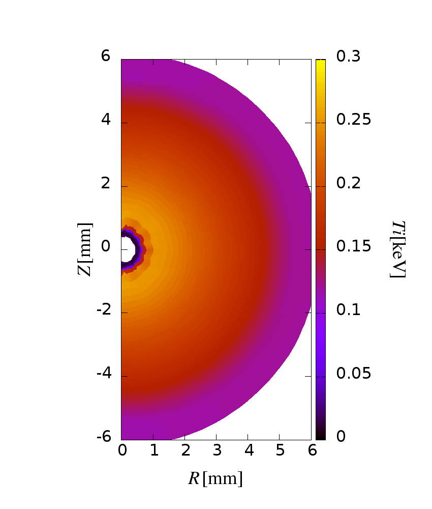
(a) with wobbling beam

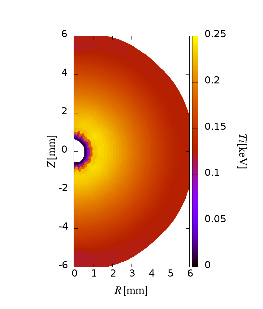
(b) w/o wobbling beam

Figure 13: Target ion temperature distributions at $t=29.0$ ns.

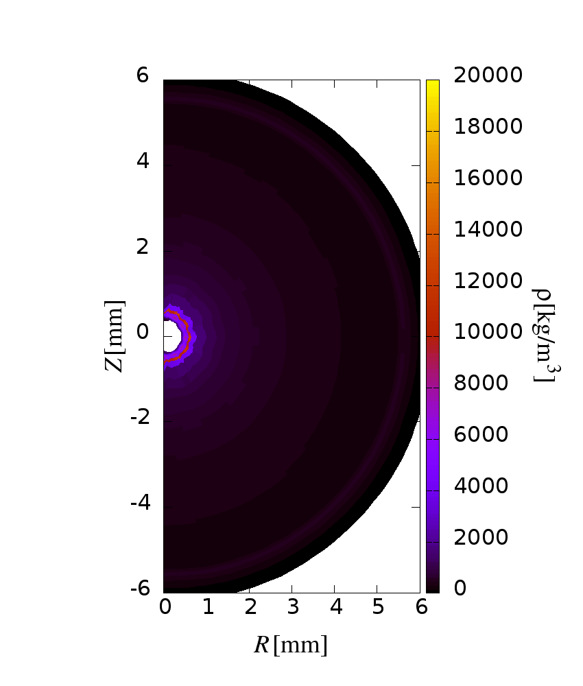
(a) with wobbling beam

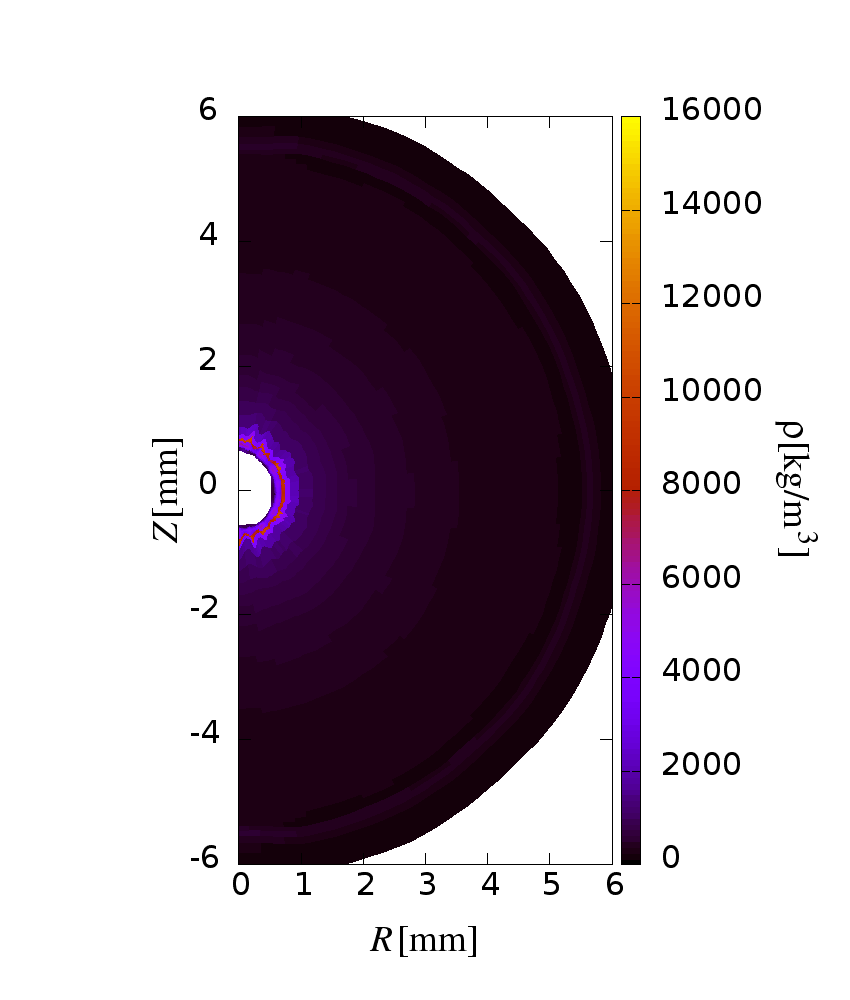
(b) w/o wobbling beam

Figure 14: Target mass density distributions at $t=29.0$ ns.

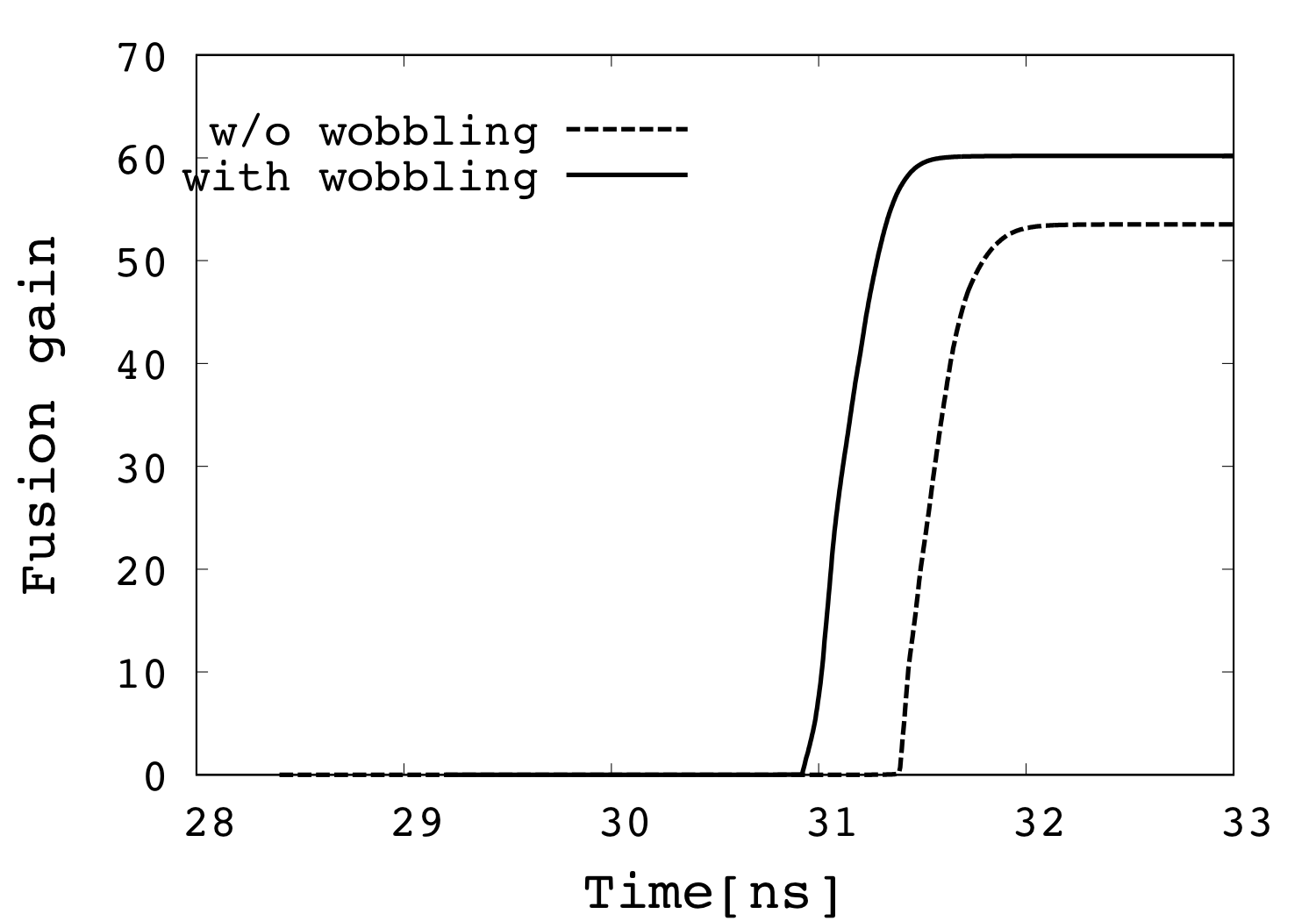
Figure 15: Fusion energy gain curves for the cases with (a solid line) and without (a dotted line) the wobbling HIBs .

7 Conclusions

We have developed and presented the O-SUKI code, which is useful to simulate 2D spherical DT fuel target implosion in HIF. The O-SUKI code consists of the HIB illumination code, the Lagrangian fluid code, the data conversion from the Lagrangian code data to the Euler code data, and the Euler code. Near the void closure phase of the DT fuel implosion, the DT fuel spatial deformation is serious. At the stagnation phase the DT fuel is compressed to about a thousand times of the solid density. Therefore, The Euler code is appropriate after the void closure phase, however the Lagrangian code is effective before the void closure time. In addition, data visualization script programs are also provided. The O-SUKI code would provide a useful tool for the integrated DT fuel target implosion simulation in HIF.

References

- [1] S. Atzeni, J. Meyer-ter-Vehn, The Physics of Inertial Fusion, Oxford University Press, 2009.
- [2] S. Kawata, K. Niu, J. Phys. Soc. Jpn. 53 (1984) 3416-3426.
- [3] S. Kawata, T. Karino, A. I. Ogoyski, Matter and Radiation at Extremes 1(2) (2016) 89-113.
- [4] I. Hofmann, Matter and Radiation at Extremes, 3(1) (2018) 1-11.
- [5] D. Böhne, I. Hofmann, G. Kessler, G.L. Kulcinski, J. Meyer-ter-Vehn, et al., Nucl. Eng. Des. 73 (2) (1982) 195-200.
- [6] T. Yamaki, et al., HIBLIC-1, Conceptual Design of a Heavy Ion Fusion Reactor, Research Information Center, Institute for Plasma Physics, Nagoya University, Report IPPJ-663, 1985.
- [7] R.W. Moir, R.L. Bieri, X.M. Chen, T.J. Dolan, M.A. Hoffman, et al., Fusion Technol. 25 (1994) 5-25.
- [8] J. F. Ziegler, J. P. Biersack, U. Littmark, The Stopping and Range of Ions in matter, volume 1, Pergamon, New York, 1985.
- [9] T.A. Mehlhorn, J. Appl. Phys. 52 (1981) 6522-6532.
- [10] D.A. Callahan-Miller, M. Tabak, Nucl. Fusion 39 (1999) 883-892.
- [11] R.C. Arnold, E. Colton, S. Fenster, M. Foss, G. Magelssen, et al., Nucl. Inst. Meth. 199 (1982) 557-561.
- [12] A.R. Piriz, A.R.N.A. Tahir, D.H.H. Hoffmann, M. Temporal, Phys. Rev. E 67 (017501) (2003) 1-3.
- [13] H. Qin, R.C. Davidson, B.G. Logan, Phys. Rev. Lett. 104 (2010) 254801.
- [14] S. Kawata, T. Sato, T. Teramoto, E. Bandoh, Y. Masubichi, et al., Laser Part. Beams 11 (1993) 757-768.
- [15] S. Kawata, T. Sato, T. Teramoto, E. Bandoh, Y. Masubichi, et al., Phys. Plasmas 19 (2012) 024503.
- [16] S. Kawata, T. Karino, Phys. Plasmas 22 (2015) 042106.
- [17] S.E. Bodner, Phys. Rev. Lett. 33 (1974) 761-764.
- [18] H. Takabe, K. Mima, L. Montierth, R.L. Morse, Phys. Fluids 28 (1985) 3676-3682.
- [19] J. Sasaki, T. Nakamura, Y. Uchida, T. Someya, K. Shimizu, M. Shitamura, T. Teramoto, A. I. Blagoev, S. Kawata, Jpn. J. Appl. Phys. 40(1) (2001) 968-971.
- [20] K. Miyazawa, A.I. Ogoyski, S. Kawata, T. Someya, T. Kikuchi, Phys. Plasmas 12 (2005) 122702-122711.
- [21] A. I. Ogoyski, et al., Comput. Phys. Commun. 157 (2004) 160-172.
- [22] A. I. Ogoyski, S. Kawata and T. Someya, Compt. Phys. Commun. 161 (2004) 143-150.
- [23] A. I. Ogoyski, S. Kawata, P. H. Popov,Compt, Phys. Commun. 181 (2010) 1332-1333.
- [24] W. D. Schulz, ”Two-Dimensional Lagrangian Hydrodynamic Difference Equations”, University of California Lawrence Radiation Laboratory Livermore, California, UCRL-6776, 1963.
- [25] N. A. Tahir, K. A. Long, E. W. Laing, J. Appl. Phys. 60 (1986) 898.
- [26] Ya. B. Zel’dovich, Yu. P. Raizer, Physics of Shock Waves and High-Temperature Hydrodynamic Phenomena, Dover Books on Physics, New York, 2002.
- [27] J. Von Neumann and R. D. Richtmyer, J. Appl. Phys. 21 (1950) 232-237.
- [28] J. P. Christianen, D. E. T. F. Ashby, and K. V. Roberts, Computer Physics Communications 7 (1974) 271-287.
- [29] A. R. Bell, Rutherford Laboratory Report, RL-80-091, 1981.
- [30] G. S. Fraley, E. J. Linnebur, R. J. Mason, R. L. Morse, Phys. Fluids, 17 (1974) 474-489.