ExoMol line lists XXXI: Spectroscopy of lowest eights electronic states of C₂

Abstract

Accurate line lists for the carbon dimer, C₂, are presented. These line lists cover rovibronic transitions between the eight lowest electronic states: $X\,{}^{1}\Sigma_{g}^{+}$, $a\,{}^{3}\Pi_{u}$, $A\,{}^{1}\Pi_{u}$, $b\,^{3}\Sigma_{g}^{-}$, $c\,^{3}\Sigma_{u}^{+}$, $d\,{}^{3}\Pi_{g}$, $B\,{}^{1}\Delta_{g}$ and $B^{\prime}\,{}^{1}\Sigma_{g}^{+}$. Potential energy curves (PECs) and transition dipole moment curves are computed on a large grid of geometries using the aug-cc-pwCVQZ-DK/MRCI level of theory including core and core-valence correlations and scalar relativistic energy corrections. The same level of theory is used to compute spin-orbit and electronic angular momentum couplings. The PECs and couplings are refined by fitting to the empirical (MARVEL) energies of ¹²C₂ using the nuclear-motion program Duo. The transition dipole moment curves are represented as analytical functions to reduce the numerical noise when computing transition line strengths. Partition functions, full line lists, Landé-factors and lifetimes for three main isotopologues of C₂ (¹²C₂,¹³C₂ and ¹²C¹³C) are made available in electronic form from the CDS (http://cdsarc.u-strasbg.fr) and ExoMol (www.exomol.com) databases.

1 Introduction

The C₂ molecule is a prominent species in a wide variety of astrophysical sources, including comets (Rousselot et al., 2012), interstellar clouds (Hupe et al., 2012), translucent clouds (Sonnentrucker et al., 2007), proto planetary nebulae (Wehres et al., 2010), cool carbon stars (Goorvitch, 1990), high-temperature stars (Vartya, 1970) and the Sun (Lambert, 1978; Brault et al., 1982). Indeed C₂ spectra are commonly used to determine the ¹²C/¹³C isotopic ratio in carbon stars (Zamora et al., 2009) and comets (Stawikowski & Greenstein, 1964).

Unusually, astronomical spectra of C₂ have been observed via several different electronic bands; those considered in this work are summarised in Figure 1. The spectroscopy of C₂ is an important tool for stellar classifications (Keenan & Morgan, 1941; Vartya, 1970; Fujita, 1980; Keenan, 1993; Gonneau, A. et al., 2017; De Mello et al., 2009) and determining the chemical composition of stars (Querci et al., 1971; Lambert et al., 1984; Goorvitch, 1990; Bakker et al., 1996; Gonneau, A. et al., 2017; Hall & Maxwell, 2008; Green, 2013; Zamora et al., 2009; Ishigaki et al., 2012; Schmidt et al., 2013) and of the Sun (Lambert, 1968; Grevesse & Sauval, 1973; Lambert, 1978; Brault et al., 1982).

Figure 1: Band systems connecting the eight lowest electronic states of C₂ considered in this work. The dashed lines represent intercombination bands.

The Swan bands of C₂ have long been known in cometary spectra (Meunier, 1911). These bands are easily detected and have been extensively studied, see Rousselot et al. (2012), for example. The Swan bands are useful to estimate the effective excitation temperatures of C₂, see, for example, Lambert & Danks (1983) and Rousselot et al. (1995). Using C₂ columns densities, Newburn & Spinrad (1984) were able to obtain C₂/O and C₂/CN ratios for 17 comets. Other observations include works on the cometary spectroscopy of C₂ are by Stawikowski & Greenstein (1964); Mayer & O’dell (1968); Owen (1973); Danks et al. (1974); Lambert & Danks (1983); Johnson et al. (1983); Newburn & Spinrad (1984); Gredel et al. (1989); Rousselot et al. (2012).

Stawikowski & Greenstein (1964) used the (1,0) Swan band to determine the ¹²C/¹³C ratio in comet Ikeya and found it similar to that observed in the solar system, ¹²C/¹³C = 89. The (1,0) band head was also used to determine the ¹²C/¹³C ratio in the comet Tago-Sato-Kosaka 1969 by Owen (1973) and the comet Kohoutek by Danks et al. (1974). Rousselot et al. (2012) used the (1,0) and (2,1) Swan bands to obtain isotope ratios for 2 comets (NEAT and LINEAR), which were again consistent with the terrestrial ratio, thus supporting the proposition that comets were created in our solar system and indicating that the ratio has not changed significantly since their birth (Rousselot et al., 2012).

Although C₂ had long been observed in spectra of cool stars and comets, the first detection in the interstellar medium (ISM) was made by Souza & Lutz (1977) using the C₂ Phillips (1,0) band in the near-infrared spectrum towards the star Cyg OB212. The $Q(2)$ line of the Phillips (2,0) band was observed by Chaffee & Lutz (1978) toward $\zeta$ Oph, after which Chaffee et al. (1980) observed 9 lines of this band toward $\zeta$ Per. The (3,0) band was observed by Van Dishoeck & Black (1986) toward $\zeta$ Oph. There have followed many other ISM observations featuring C₂ spectra (Hobbs, 1979, 1981; Hobbs & Campbell, 1982; Hobbs et al., 1983; van Dishoeck & de Zeeuw, 1984; Van Dishoeck & Black, 1986; Black & van Dishoeck, 1988; Federman & Huntress, 1989; Snow & McCall, 2006; Sonnentrucker et al., 2007; Wehres et al., 2010; Hupe et al., 2012).

Lebourlot & Roueff (1986) suggested that the $a\,{}^{3}\Pi_{u}$ – $X\,{}^{1}\Sigma_{g}^{+}$ intercombination band might be observable in the ISM. So far such lines have yet to be observed in the ISM and attempts to observe them in a comet also failed (Rousselot et al., 1998). However, this band has recently been detected in the laboratory (Chen et al., 2015), allowing a precise determination of the singlet-triplet separation (Furtenbacher et al., 2016). Our line list provides accurate wavelengths and transition intensities for these lines based on rovibronic mixing between states.

On Earth C₂ is abundant in flames, explosions, combustion sources, electrical hydrocarbon discharges and photolysis processes (Hornkohl et al., 2011). The C₂ spectrum (especially the Swan band $d$–$a$) is commonly used to monitor carbon-based plasmas including industrial applications; see, for example, Jönsson et al. (2007); Al-Shboul et al. (2013); Bauer et al. (2017) and references therein.

Although numerous transition bands have been studied experimentally, the accuracy of the line positions has been considerably improved in recent years by application of jet expansion, modern lasers and Fourier transform techniques. Here we focus on the most accurate measured transitions, which involve the first eight lowest electronic states of C₂, see Figure 1. A summary of experimental work on the bands linking these states is presented below through the Phillips, Swan, Ballik-Ramsay, Bernath and Duck systems. Furtenbacher et al. (2016) recently undertook a comprehensive assessment of high-resolution laboratory studies of C₂ spectra; they derived empirical energy levels using the MARVEL (measured active rotation vibration energy levels) procedure which are used extensively in the present work.

There have been extensive theoretical studies involving the eight lowest electronic states of C₂; here we discuss only the most recent works. Because of the near degeneracies among the electron configurations along the whole range of internuclear separations, the potential energy curves (PECs) lie very close together, even near the equilibrium geometry, and several PECs undergo avoided crossings. This means that traditional single-reference methods are unable to provide quantitatively acceptable results for the functions dependent upon the interatomic distance (Abrams & Sherrill, 2004; Sherrill & Piecuch, 2005).

Systematic high level ab initio analysis of the $J=0$ vibrational manifolds including also the ¹²C¹³C and ¹³C₂ isotopologues was performed for the $A\,{}^{1}\Pi_{u}$ and $X\,{}^{1}\Sigma_{g}^{+}$ states by Zhang et al. (2011), who computed PECs of C₂ at the multi-reference configuration interaction (MRCI) (Werner & Knowles, 1988) level of theory in conjunction with the aug-cc-pV6Z basis set, using complete active space self-consistent field (CASSCF) (Roos & Taylor, 1980; Werner & Knowles, 1985) reference wave functions.

Highly accurate potential energy curves, transition dipole moment functions, spectroscopic constants, oscillator strengths and radiative lifetimes were obtained for the Phillips, Swan, Ballik-Ramsay and Duck systems by Kokkin et al. (2007) using the CASSCF and subsequent MRCI computational approach including higher order corrections. Schmidt & Bacskay (2007) improved the aforementioned computational methodology by computation of MRCI transition dipole moments between these four systems. Accurate ab initio calculations of three PECs of C₂ at the complete basis set limit were reported by Varandas (2008).

Brooke et al. (2013) presented an empirical line list for the Swan system of C₂ ($d\,{}^{3}\Pi_{g}$–$a\,{}^{3}\Pi_{u}$) which included vibrational bands with $v^{\prime}=0-10$ and $v^{\prime\prime}=0-9$, and rotational states with $J$ up to 96, based on an accurate ab initio (MRCI) transition dipole moment $d$–$a$ curve. The opacity database of Kurucz (2011) contains a C₂ line list for several electronic bands; Ballik-Ramsay, Swan, Fox-Herzberg ($e\,{}^{3}\Pi_{g}$ – $a\,{}^{3}\Pi_{u}$) and Phillips.

Experimental lifetimes of specific vibronic states of C₂ have been reported by Smith (1969); Curtis et al. (1976); Bauer et al. (1985); Bauer et al. (1986); Naulin et al. (1988); Erman & Iwame (1995) and Kokkin et al. (2007). These observations provide an important test of any spectroscopic model for the system. Brooke et al. (2013) reported theoretical lifetimes for the Swan band which were in good agreement with experimental values.

The ExoMol project aims to provide line lists for all molecules of importance for the atmospheres of exoplanets and cool stars (Tennyson & Yurchenko, 2012; Tennyson et al., 2016b). Given the astrophysical importance of C₂ and the lack of a comprehensive line list for the molecule, it is natural that C₂ should be treated as part of the ExoMol project. Here we use the program Duo (Yurchenko et al., 2016a) to produce line lists for the eight electronic states ($X\,{}^{1}\Sigma_{g}^{+}$, $A\,{}^{1}\Pi_{u}$, $B\,{}^{1}\Delta_{g}$, $B^{\prime}\,{}^{1}\Sigma_{g}^{+}$, $a\,{}^{3}\Pi_{u}$, $b\,^{3}\Sigma_{g}^{-}$, $c\,^{3}\Sigma_{u}^{+}$  and $d\,{}^{3}\Pi_{g}$) of three isotopologues of C₂. The electronic bands connecting these states are summarized in Fig. 1. The line lists are computed using high level ab initio transition dipole moments of C₂, MRCI/aug-cc-pwCVQZ-DK and empirical potential energy, spin-orbit, electronic angular momenta, Born-Oppenheimer breakdown, spin-spin, spin-rotation and $\Lambda$-doubling curves (see below for description of the curves taken into account). These empirical curves were obtained by refining ab initio curves using a recent set of experimentally-derived (MARVEL) term values of C₂ (Furtenbacher et al., 2016). This methodology has been used for similar studies as part of the ExoMol project including the diatomic molecules AlO (Patrascu et al., 2015), ScH (Lodi et al., 2015), CaO (Yurchenko et al., 2016b), PO and PS (Prajapat et al., 2017), VO McKemmish et al. (2016), NO (Wong et al., 2017), NS and SH (Yurchenko et al., 2018b), SiH (Yurchenko et al., 2018a), and AlH (Yurchenko et al., 2018c).

2 Theoretical approach

2.1 Electronic structure computations

The presence of spin, orbital and rotational angular moment results in complicated and extensive couplings between electronic states. How these are treated formally and their non-perturbative inclusion in the calculation of rovibronic spectra of diatomic molecules is the subject of a recent topical review by two of us (Tennyson et al., 2016a); this review provides a detailed, formal description of the various coupling curves considered below.

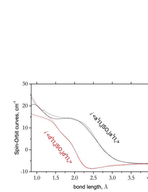
Figure 3: Diagonal spin-orbit curves of C₂ between the $a\,{}^{3}\Pi_{u}$ and $d\,{}^{3}\Pi_{g}$. The ab initio curves are shown using dashed line, while the refined curves are given by solid lines. The empirical $d\,{}^{3}\Pi_{g}$ SOC was produced by morphing the ab initio curve, while the $a\,{}^{3}\Pi_{u}$ SOC was obtained by refining the ab initio parameters.

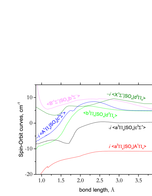
Figure 4: Ab initio $a$–$A$, $a$–$c$, $B^{\prime}$–$b$, $b$–$d$, $X$–$d$ and $A$–$c$ spin-orbit curves of C₂. These curves were not refined.

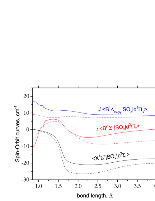
Figure 5: Spin-orbit $X$–$b$, $B$–$d$ and $B^{\prime}$–$d$ curves of C₂. The ab initio curves are shown using dashed line, while the refined curves are given by solid curves.

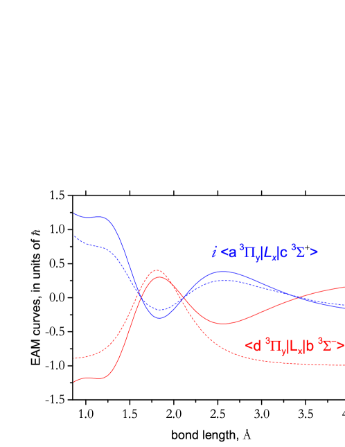
Figure 6: Refined $a$–$c$ and $d$–$b$ EAM curves of C₂. The ab initio curves are shown using dashed line, while the refined curves are given by solid curves.

The PECs, spin-orbit coupling curves (SOCs), electronic angular momentum curves (EAMCs) and the transition dipole moment curves (TDMs) were computed at the MRCI level of theory, using reference wave functions from a CASSCF with all single and double excitations included, in conjunction with the augmented correlation-consistent polarized aug-cc-pwCVQZ-DK Dunning type basis set (Dunning, 1989; Woon & Dunning, 1993; Peterson & Dunning, 2002), plus Duglas-Kroll corrections and core-correlation effects as implemented in MOLPRO (Werner et al., 2012). The complete active space is defined by (3,1,1,0,3,1,1,0) in the D_2h symmetry group employed by MOLPRO, which corresponds to the $A_{g}$, $B_{3u}$, $B_{2u}$, $B_{1g}$, $B_{1u}$, $B_{2g}$, $B_{3g}$ and $A_{u}$ irreducible representations of this group, respectively. The initial grid included about 400 points ranging from 0.7 to 10 Å, however some geometries close to the curve crossings did not converge and were then excluded. Some of the ab initio curves are shown in Figs. 2 – 9. Our $a$–$d$ transition dipole moment curve compares well with that computed by Brooke et al. (2013) who used it to produce their C₂ line list for the Swan system.

2.2 Solution of the rovibronic problem

We used the program Duo (Yurchenko et al., 2016a) to solve the fully coupled Schrödinger equation for eight lowest electronic states of C₂, single and triplet: $X\,{}^{1}\Sigma_{g}^{+}$, $A\,{}^{1}\Pi_{u}$, $B\,{}^{1}\Delta_{g}$, $B^{\prime}\,{}^{1}\Sigma_{g}^{+}$, $a\,{}^{3}\Pi_{u}$, $b\,^{3}\Sigma_{g}^{-}$, $c\,^{3}\Sigma_{u}^{+}$  and $d\,{}^{3}\Pi_{g}$. The vibrational basis set was constructed by solving eight uncoupled Schröninger equations using the sinc DVR method based on the grid of equidistant 401 points covering the bond lengths between 0.85 and 4 Å. The vibrational basis sets sizes were 60, 30, 30, 30, 40, 40, 30 and 30 for $X\,{}^{1}\Sigma_{g}^{+}$, $A\,{}^{1}\Pi_{u}$, $B\,{}^{1}\Delta_{g}$, $B^{\prime}\,{}^{1}\Sigma_{g}^{+}$, $a\,{}^{3}\Pi_{u}$, $b\,^{3}\Sigma_{g}^{-}$, $c\,^{3}\Sigma_{u}^{+}$  and $d\,{}^{3}\Pi_{g}$, respectively.

Duo employs Hund’s case a formalism: rotational and spin basis set functions are the spherical harmonics $|J,\Omega\rangle$ and $|S,\Sigma\rangle$, respectively. For the nuclear-motion step of the calculation, the electronic basis functions $|{\rm State},\Lambda\rangle$ are defined implicitly by the matrix elements of the SO, EAM coupling and TDM as computed by MOLPRO. Note that the couplings and TDMs had to be made phase-consistent (Patrascu et al., 2014) and transformed to the symmetrized $\Lambda$-representation, see Yurchenko et al. (2016a).

2.3 Potential energy curves

Our PECs are fully empirical (reconstructed through the fit to the experimental data). To represent the potential energy curves the following two types of functions were used.

For the simpler PECs that do not exhibit avoided crossing ($A\,{}^{1}\Pi_{u}$, $B\,{}^{1}\Delta_{g}$, $a\,{}^{3}\Pi_{u}$, $b\,^{3}\Sigma_{g}^{-}$ and $c\,^{3}\Sigma_{u}^{+}$) we used the extended Morse oscillator (EMO) functions (Lee et al., 1999) for both ab initio and refined PECs.

In this case a PEC is given by

$$V(r)=V_{\rm e}\;\;+\;\;(A_{\rm e}-V_{\rm e})\left[1\;\;-\;\;\exp\left(-\sum_{k=0}^{N}B_{k}\xi_{p}^{k}(r-r_{\rm e})\right)\right]^{2},$$ (1)

where $A_{\rm e}-V_{\rm e}$ is the dissociation energy, $r_{\rm e}$ is an equilibrium distance of the PEC, and $\xi_{p}$ is the Šurkus variable given by:

$$\xi_{p}=\frac{r^{p}-r^{p}_{\rm e}}{r^{p}+r^{p}_{\rm e}}.$$ (2)

The corresponding expansion parameters are obtained by fitting to the empirical (MARVEL) energies from Furtenbacher et al. (2016).

For the three states with avoided crossing, $X\,{}^{1}\Sigma_{g}^{+}$, $B^{\prime}\,{}^{1}\Sigma_{g}^{+}$ and $d\,{}^{3}\Pi_{g}$ (see Fig. 2) a diabatic representation of two coupled EMO PECs was used. In this representation the PEC is obtained as a root of a characteristic $2\times 2$ diabatic matrix

$$\bf{A}=\left(\begin{array}[]{cc}V_{1}(r)&W(r)\\ W(r)&V_{2}(r)\end{array}\right),$$ (3)

where $V_{1}(r)$ and $V_{2}(r)$ are given by the EMO potential function in Eq. (1). The coupling function $W(r)$ is given by

$$W(r)=W_{0}+\frac{\sum_{i\geq 0}w_{i}(r-r_{\rm cr})^{i}}{\cosh[\beta(r-r_{\rm cr})]},$$ (4)

where $r_{\rm cr}$ is a crossing point. The two eigenvalues of the matrix $\bf{A}$ are given by

$$V_{\rm low}(r) = \frac{V_{1}(r)+V_{2}(r)}{2}-\frac{\sqrt{[V_{1}(r)-V_{2}(r)]^{2}+4\,W^{2}(r)}}{2},$$ (5)

$$V_{\rm upp}(r) = \frac{V_{1}(r)+V_{2}(r)}{2}+\frac{\sqrt{[V_{1}(r)-V_{2}(r)]^{2}+4\,W^{2}(r)}}{2}.$$ (6)

For each pair of states, only one component is taken, $V_{\rm low}$ for $X\,{}^{1}\Sigma_{g}^{+}$ and $d\,{}^{3}\Pi_{g}$ and $V_{\rm upp}$ for $B^{\prime}\,{}^{1}\Sigma_{g}^{+}$, and the other component is ignored. For example, the coupled $X$–$B^{\prime}$ system is treated as two independent diabatic systems in Eq. (3), as we could not obtain a consistent model with only one pair of the $X$ and $B^{\prime}$ curves. In case of the $X\,{}^{1}\Sigma_{g}^{+}$ state, the upper component, formally representing the $B^{\prime}\,{}^{1}\Sigma_{g}^{+}$ state, is only used as a dummy PEC. The actual $B^{\prime}\,{}^{1}\Sigma_{g}^{+}$ PEC is taken as the upper component with different $V_{\rm low}$. The latter is also a dummy PEC and disregarded from the rest of the calculations. In this decoupled way we could achieve a more stable fit.

The expansion parameters, including the corresponding equilibrium bond lengths $r_{\rm e}$ appearing in Eqs. (1)–(4) are obtained by fitting to the experimentally-derived energies. The dissociation asymptote $A_{\rm e}$ in all cases was first varied and then fixed the value 50937.91 cm^-1 (6.315 eV) for all but the $d\,{}^{3}\Pi_{g}$ PEC, for which it was refined to obtain 62826.57 cm^-1 (7.789 eV) for better accuracy. To compare, the experimental value of $D_{0}$ = 6.30 $\pm 0.02$ eV ($D_{{\rm e}}$ $\sim$ 6.41 eV) was determined by Urdahl et al. (1991). The best ab initio values of $D_{\rm e}$ of C₂ from the literature include 6.197 eV by Feller & Sordo (2000) and 6.381 eV by Varandas (2008). The lowest asymptote $A_{\rm e}$ correlates with the ${}^{3}P$+${}^{3}P$ limit (Martin, 1992), while the next is the ${}^{3}P$+${}^{1}D$ limit (+1.26 eV). Our zero-point-value is 924.02 cm^-1.

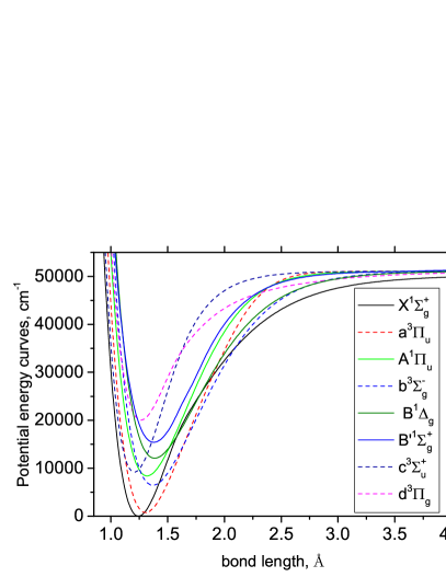
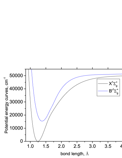
Figure 2: The eight refined potential energy curves of C₂ (left) and the avoided crossing between the $X\,{}^{1}\Sigma_{g}^{+}$ and $B^{\prime}\,{}^{1}\Sigma_{g}^{+}$ states in the adiabatic representation (right).

The effect of the avoiding crossings on the shape of the $X\,{}^{1}\Sigma_{g}^{+}$, $B^{\prime}\,{}^{1}\Sigma_{g}^{+}$ and $d\,{}^{3}\Pi_{g}$ PECs is illustrated in Fig. 2. It is clear that simple one-curve expansions would be problematic for these states. This effect has been studied in detail by Varandas (2008, 2009).

2.4 Couplings

In the refinement of the SO and EAM coupling we use the ab initio curves, which are ‘morphed’ at the ab initio grid points using the following expansion:

$$F(r)=\sum^{N}_{k=0}B_{k}\,z^{k}(1-\xi_{p})+\xi_{p}\,B_{\infty},$$ (7)

where $z$ is either taken as the Šurkus variable $z=\xi_{p}$ or a damped-coordinate given by:

$$z=(r-r_{\rm ref})\,e^{-\beta_{2}(r-r_{\rm ref})^{2}-\beta_{4}(r-r_{\rm ref})^{4}},$$ (8)

see also Prajapat et al. (2017) and Yurchenko et al. (2018a). Here $r_{\rm ref}$ is a reference position equal to $r_{\rm e}$ by default and $\beta_{2}$ and $\beta_{4}$ are damping factors. When used for morphing, the parameter $B_{\infty}$ is usually fixed to 1. The $B_{\infty}$ parameters should in principle correspond to the atomic limit of the corresponding couplings, however we have not attempted to apply any such constraints. Due to very steep character of the potential energy curves, the long-range part of the coupling curves has no impact on the states we consider.

Some of the coupling curves have complex shapes due to, for example, avoiding crossings. This complexity is assumed to be covered by the morphing procedure, as morphed curves should inherit the shape of the parent function.

The spin-spin and spin-rotational couplings were introduced for the states $a\,{}^{3}\Pi_{u}$, $c\,^{3}\Sigma_{u}^{+}$ and $d\,{}^{3}\Pi_{g}$ and also modelled using the expansion given by Eq. (7). The final curves, which are fully empirical, are shown in Fig. 7.

The $\Lambda$-doubling effects in $a\,{}^{3}\Pi_{u}$ and $d\,{}^{3}\Pi_{g}$ were obtained empirically using effective $\Lambda$-doubling functions, the ($o$+$p$+$q$) and ($p$+2$q$) coupling operators (Brown & Merer, 1979) as given by:

$$\hat{H}_{opq} = \frac{1}{2}\alpha_{\rm opq}^{\rm LD}(r)\left(\hat{S}_{+}^{2}+\hat{S}_{-}^{2}\right),$$ (9)

$$\hat{H}_{\rm p2q} = -\frac{1}{2}\alpha_{p2q}^{\rm LD}(r)\left(\hat{J}_{+}\hat{S}_{+}+\hat{J}_{-}\hat{S}_{-}\right).$$ (10)

The latter operator is limited to linear $\hat{J}$-dependence, which is justified for the heavy molecule like C₂. In this case for $\alpha_{p2q}^{\rm LD}(r)$ and $\alpha_{\rm opq}^{\rm LD}(r)$ we use the Šurkus-type expansion as in Eq. (7). The empirical $\Lambda$-doubling curves of C₂ are shown in Fig. 8. We used these couplings to improve the fit for the states $a\,{}^{3}\Pi_{u}$ and $d\,{}^{3}\Pi_{g}$.

To allow for rotational Born-Oppenheimer breakdown (BOB) effects (Le Roy, 2017), the vibrational kinetic energy operator for each electronic state was extended by

$$-\frac{\hbar^{2}}{2\mu r^{2}}\to-\frac{\hbar^{2}}{2\mu r^{2}}\left(1+g^{\rm BOB}(r)\right),$$ (11)

where the unitless BOB functions $g^{\rm BOB}$ are represented by the polynomial

$$g^{\rm BOB}(r)=\left[(1-\xi_{p})\sum_{k\geq 0}^{N_{T}}A_{k}\xi_{p}^{k}+\xi_{p}A_{\rm\infty}\right],$$ (12)

where $\xi_{p}$ as the S̆urkus variable and $p$, $A_{k}$ and $A_{\rm\infty}$ are adjustable parameters. This representation was used for the $d\,{}^{3}\Pi_{g}$ state only, which appeared to be most difficult to fit.

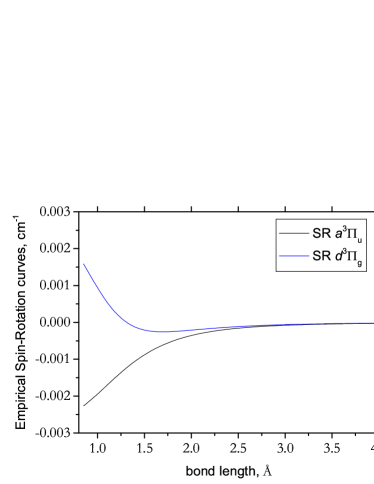
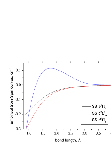
Figure 7: Empirical curves of C₂: spin-rotational (left) and spin-spin (right) curves representing the states $a\,{}^{3}\Pi_{u}$, $c\,^{3}\Sigma_{u}^{+}$ and $d\,{}^{3}\Pi_{g}$.

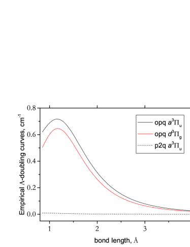
Figure 8: Empirical the $\Lambda$-doubling curves used for $a\,{}^{3}\Pi_{u}$ and $d\,{}^{3}\Pi_{g}$(left) and a Born-Oppenheimer breakdown curve used for $d\,{}^{3}\Pi_{g}$ (right) of C₂.

2.5 Dipole moment curves

The electronic dipole pure rotation and rotation-vibration transitions are forbidden for the homonuclear molecule C₂, so are the transitions between electronic states with $\Delta\Lambda>1$ or $\Delta\Lambda=0$ for $\Sigma$ states. There are six (electric-dipole) allowed electronic bands between lowest eight electronic states of C₂ shown in Fig. 1. The corresponding electronic transition dipole moments are shown in Fig. 9. These ab initio TDMCs were represented analytically using the damped-$z$ expansion in Eq. (7). This was done in order to reduce the numerical noise in the calculated intensities for high overtones, see recent recommendations by Medvedev et al. (2016). The corresponding expansion parameters as well as their grid representations can be found in the Duo input files provided as supplementary data.

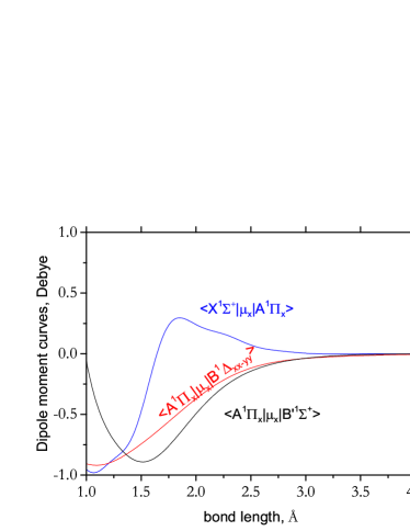
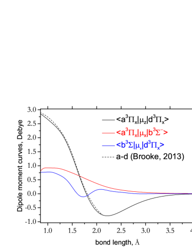
Figure 9: Dipole moment curves of C₂ between the singlet states $X$–$A$, $A$–$B$ and $A$–$B^{\prime}$ (left) and between triplet states $a$–$d$, $a$–$b$ and $b$–$d$. The ab initio $a$–$d$ TDMC used by Brooke et al. (2013) is also shown.

3 Refinement

In the refinements we used the experimentally-derived energies obtained by Furtenbacher et al. (2016) using the MARVEL approach. These energies were based on a comprehensive set of experimental frequencies collected from a large number of sources which are listed in Table 1. Some statistics about the experimental energies is shown in Table 2. For full details of the MARVEL procedure as well as descriptions of the experimental data see Furtenbacher et al. (2016).

Table 1: Experimental sources used to generate the MARVEL energies of C₂ (Furtenbacher et al., 2016).

System	Source
Phillips $A\,{}^{1}\Pi_{u}$$-$$X\,{}^{1}\Sigma_{g}^{+}$	Chen et al. (2015); Davis et al. (1988b); Douay et al. (1988a); Chauville et al. (1977)
	Ballik & Ramsay (1963); Petrova & Sinitsa (2006); Chan et al. (2004); Nakajima & Endo (2013),
Bernath $B\,{}^{1}\Delta_{g}$ $-$ $A\,{}^{1}\Pi_{u}$	Douay et al. (1988b); Chen et al. (2016)
Bernath $B^{\prime}\,{}^{1}\Sigma_{g}^{+}$$-$$A\,{}^{1}\Pi_{u}$	Douay et al. (1988b)
Freymark $E\,{}^{1}\Sigma_{g}^{+}$$-$$A\,{}^{1}\Pi_{u}$	Sorkhabi et al. (1997); Freymark (1951)
Ballik–Ramsay $b\,^{3}\Sigma_{g}^{-}$$-$$a\,{}^{3}\Pi_{u}$	Chen et al. (2015); Yan et al. (1985); Roux et al. (1985); Amiot et al. (1979)
	Davis et al. (1988a); Petrova & Sinitsa (2006); Bornhauser et al. (2011)
Swan $d\,{}^{3}\Pi_{g}$$-$$a\,{}^{3}\Pi_{u}$	Nakajima & Endo (2013, 2014); Bornhauser et al. (2013); Yeung et al. (2013)
	Tanabashi et al. (2007); Phillips (1948a); Tanabashi & Amano (2002); Kaniki et al. (2003)
	Curtis & Sarre (1985); Prasad & Bernath (1994); Amiot (1983); Lloyd & Ewart (1999)
Fox–Herzberg e ${}^{3}\Pi_{\rm g}-$$a\,{}^{3}\Pi_{u}$	Hardwick & Winicur (1986); Phillips (1948b); Brockhinke et al. (1998)
Duck $d\,{}^{3}\Pi_{g}$$-$$c\,^{3}\Sigma_{u}^{+}$	Chan et al. (2013); Nakajima & Endo (2013, 2014); Joester et al. (2007)
Krechkivska–Schmidt $4^{3}\Pi_{\rm g}-$ $a$	Krechkivska et al. (2015)
Interconnection $a\,{}^{3}\Pi_{u}$$-$$X\,{}^{1}\Sigma_{g}^{+}$	Chen et al. (2015)
$A\,{}^{1}\Pi_{u}$$-$$b\,^{3}\Sigma_{g}^{-}$	Chen et al. (2015)
$1~{}^{5}\Pi_{\rm g}-$ $a\,{}^{3}\Pi_{u}$	Bornhauser et al. (2011)
Radi–Bornhauser $1^{5}\Pi_{\rm u}-1^{5}\Pi_{\rm g}$	Bornhauser et al. (2015)

The final model comprises 89 parameters appearing in the expansions from Eqs. (1,4,7) obtained by fitting to 4900 MARVEL energy term values of ¹²C₂ using Duo. The robust weighting method of Watson (2003) was used to adjust the fitting weights. During the fit, in order to avoid unphysically large distortions, the SOC and EAMS curves were constrained to the ab initio shapes using the simultaneous fit approach (Yurchenko et al., 2003). The MARVEL energies were correlated to the theoretical values using the Duo assignment procedure, which is based on the largest basis function contribution (Yurchenko et al., 2016a). One of the main difficulties in controlling the correspondence between the theoretical (Duo) and experimental energies in case of such a complex, strongly coupled systems is that the relative order of the computed energies can change during the fit, in this case automatic assignment is especially helpful. For some C₂ resonance states it was necessary to use also the second largest coefficients to resolve possible ambiguities. However, even this did not fully prevent accidental re-ordering of states, especially the assignment of the different $\Omega$ components of the triplet $a$ and $d$ states appeared to be very unstable and difficult to control. In such cases, as the final resort for preventing disastrous fitting effects, states exhibiting too large errors (typically $>$ 8 cm^-1) were removed from the fit, which, together with the second-largest-coefficient assignment feature are new implementations in Duo. One of the artifacts of the largest-contribution assignment is that it can fail for the vibrational quantum numbers at high rotational excitations $J$. Our vibrational basis functions, generated as eigensolutions of the pure, uncoupled $J=0$, Schrödinger equations, become less efficient for high $J$ ($>50$). This is because of the centrifugal distortion term in the Hamiltonian, which becomes large and thus distorts the effective shape of the interaction potential substantially. The rovibronic eigenfunctions in this case are a complicated mixture of the $J=0$ vibrational contributions with no distinct large contributions. The typical situation at high rotational excitations ($J>50$) is that the rovibronic eigenfunctions consist of a large number of similar vibrational contributions, which make the largest-coefficient assignment of the quantum number $v$ meaningless. Therefore, we treated the vibrational assignment differently: for each value of $J$, the vibrational quantum number $v$ was assigned by simply counting states of the same electronic term and $\Omega$-component. This is another new feature in Duo implemented in order to improve the vibrational assignment of the states with high values $J$.

Table 2: Some statistics of the experimental term values of C₂ used in this work to refine the model.

State	$v_{\rm max}$	$J_{\rm max}$
$X\,{}^{1}\Sigma_{g}^{+}$	9	74
$A\,{}^{1}\Pi_{u}$	16	75
$B\,{}^{1}\Delta_{g}$	8	50
$B^{\prime}\,{}^{1}\Sigma_{g}^{+}$	3	32
$a\,{}^{3}\Pi_{u}$	14	86
$b\,^{3}\Sigma_{g}^{-}$	8	74
$c\,^{3}\Sigma_{u}^{+}$	7	24
$d\,{}^{3}\Pi_{g}$	12	87

It should be noted that not all experimentally-derived MARVEL energies in our fitting set are supported by multiple transitions and are therefore not equally reliable. Furthermore, in some cases there is no agreement between different experimental sources of C₂ spectra. A particular example is the $d$–$a$ study by Bornhauser et al. (2011) who pointed out a 1–2 cm^-1 discrepancies with values from a previous study by Tanabashi et al. (2007) for the $P_{1}(5)$ and $R_{1}(5)$ lines $(v^{\prime}=6,v^{\prime\prime}=5)$. We obtained similar residuals for these two transitions.

The root-mean-square (rms) errors for individual vibronic states are listed in Table 3. An rms error as an averaged quantity does not fully reflect the full diversity of the quality of the results, caused mostly by the complexity of the couplings, which we could not fully describe. Figs. 10 and 11 present a detailed overview of the Obs.$-$Calc. residuals for individual rovibronic states. Considering the avoided crossings and other complexity of the system, the generally small residues obtained represent a huge achievement. The final C₂ model is provided as Duo input files as part of the supplementary material and can be also found at www.exomol.com.

Table 3: Rms errors (cm^-1) for obs.$-$calc. residuals achieved in the fit for individual vibronic states.

$v$	$X$		$v$	$a$		$v$	$A$		$v$	$b$		$v$	$c$		$v$	$d$		$v$	$B$		$v$	$B^{\prime}$
0	0.01		0	0.16		0	0.26		0	0.09		0	0.19		0	0.19		0	0.01		0	0.02
1	0.01		1	0.02		1	0.33		1	0.14		1	0.74		1	0.09		1	0.07		1	0.06
2	0.16		2	0.06		2	0.35		2	0.13		2	0.23		2	0.17		2	0.06		2	0.31
3	0.33		3	0.05		3	0.26		3	0.07		3	0.21		3	0.44		3	0.05		3	0.10
4	0.36		4	0.08		4	0.22		4	0.07					4	0.33		4	0.03
5	0.29		5	0.13		5	0.22		5	0.14					5	0.28		5	0.01
6	0.31		6	0.08		6	0.33		6	0.15					6	0.70		6	0.04
7	0.04		7	0.72		7	0.07		7	0.10					7	0.31		7	0.04
8	0.01		8	0.67		8	0.10		8	0.13					8	0.48		8	0.18
9	1.80		9	0.32		9	0.20								9	1.00
			10	0.16		10	0.25								10	0.54
			11	0.34		11	0.29								11	0.82
			12	0.80		12	0.26								12	0.44
			13	2.43		13	0.19								13

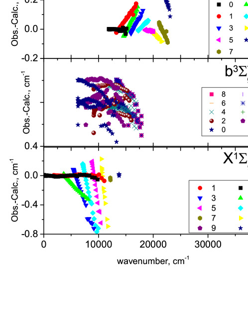
Figure 10: Obs.$-$calc. residuals for individual vibronic bands of C₂: $g$-states.

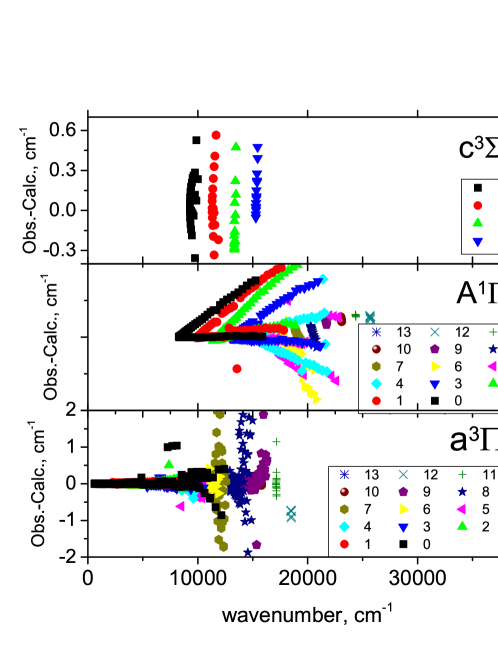
Figure 11: Obs.$-$calc. residuals for individual vibronic bands of C₂: $u$-states.

4 Line lists

The line lists for three isotopologues of the carbon dimer, ¹²C₂, ¹³C₂ and ¹²C¹³C were computed using the refined model of the eight lowest electronic states and the ab initio transition DMCs. The line lists, called 8states, cover the wavelength region up to 0.25 $\mu$m, $J=0\ldots 190$. The upper state energy term values were truncated at 50 000 cm^-1. The lower state energy threshold was set to 30 000 cm^-1 so one can assume that the other electronic states from the region below 50 000 cm^-1 (1${}^{5}\Pi_{g}$, $C\,{}^{1}\Pi_{g}$, $C^{\prime}\,{}^{1}\Pi_{g}$, $D\,{}^{1}\Sigma_{u}^{+}$ and $e\,{}^{3}\Pi_{g}$) are not populated. The vibrational excitation coverage for each electronic state was defined based on the convergence and completeness to include all bound states below the first dissociation limit. We did not have problems with the numerical noise in production of overtone intensities since they are simply forbidden, as are any transitions within the same electronic states, therefore no transition dipole moment cutoffs were applied.

The homonuclear molecule C₂ belongs to the infinite point symmetry group ${\mathcal{D}}_{\infty{\rm h}}$, which is also the group used in classification of the electronic terms. The total rovibronic state spans a finite symmetry group ${\mathcal{D}}_{\infty{\rm h}}$(M) with four elements $E$ (the identity), $(12)$ (exchange of the identical nuclei), $E^{*}$ (inversion), and $(12)^{*}$ (Bunker et al., 1997; Bunker & Jensen, 1998). The irreducible representations of ${\mathcal{D}}_{\infty{\rm h}}$(M) are $\Sigma_{g}^{+}$, $\Sigma_{g}^{-}$, $\Sigma_{u}^{+}$ and $\Sigma_{u}^{-}$. For energy calculations Duo uses the ${\mathcal{C}}_{\infty{\rm v}}$(M) group to symmetrize its basis both for homonuclear and heteronuclear systems. This group has two elements, $\Sigma^{+}$ and $\Sigma^{-}$, depending on whether the corresponding property is symmetric or antisymmetric when the molecule is inverted. In case of homonuclear ¹²C₂, the missing symmetry is the permutation of the nuclei, which introduces additional elements $g$ and $u$. This does not affect the energy calculations as the absence of corresponding couplings between $g$ and $u$ is guaranteed by construction. However, it is important to use the proper symmetry for intensities mainly due to the selection rules imposed by the nuclear spin statistics associated with different irreducible representations. For the homonuclear molecules like C₂ we therefore have to further classify the rovibronic states according to $g$ and $u$. This is done by simply adopting the corresponding symmetry of the electronic terms.

The carbon atom ¹²C has a zero nuclear spin. This gives rise to the zero statistical weights $g_{\rm ns}$ for the $\Sigma_{g}^{-}$ and $\Sigma_{u}^{+}$ states, while the other two irreducible representations have $g_{\rm ns}=1$. The statistical weights in case of ¹³C₂ are $g_{\rm ns}=$ 1,1,3 and 3 for $\Sigma_{g}^{+}$, $\Sigma_{u}^{-}$, $\Sigma_{g}^{-}$ and $\Sigma_{u}^{+}$, respectively. For ¹³C¹²C, all states have $g_{\rm ns}=2$. Note ExoMol follows the HITRAN convention (Gamache et al., 2017) and includes the full nuclear-spin degenarcy in the partition function. Other selection rules for the electronic dipole transitions are:

$$+\leftrightarrow-,\quad g\leftrightarrow u,\quad J^{\prime}-J^{\prime\prime}=0,\pm 1.$$

The ¹²C₂ line list contains 44 189 states and 6 080 920 transitions, while the ¹³C₂ and ¹²C¹³C line lists comprise 94 003/13 361 992 and 91 067/1 2743 954 states/transitions, respectively.

The line lists include lifetimes and Lánde-$g$ factors. Extracts from the line lists are given in Tables 4 and 5. In the final .states file the theoretical (Duo) energy term values were replaced with the experimentally derived (MARVEL) values where available and indicated by a label m.

Table 4: Extract from the .states file for ¹²C₂.

$n$	$\tilde{E}$	$g_{\rm tot}$	$J$	$\tau$	$g$-Landé	$+/-$	e/f	State	$v$	$\Lambda$	$\Sigma$	$\Omega$	m/d
1	0.000000	1	0	Inf	0.000000	+	e	X1Sigmag+	0	0	0	0	m
2	1827.486182	1	0	1.71E+03	0.000000	+	e	X1Sigmag+	1	0	0	0	m
3	3626.681492	1	0	1.08E+03	0.000000	+	e	X1Sigmag+	2	0	0	0	m
4	5396.686466	1	0	1.34E+01	0.000000	+	e	X1Sigmag+	3	0	0	0	m
5	6250.149530	1	0	1.81E-05	0.000000	+	e	b3Sigmag-	0	0	0	0	m
6	7136.349911	1	0	6.52E-01	0.000000	+	e	X1Sigmag+	4	0	0	0	m
7	7698.252879	1	0	1.47E-05	0.000000	+	e	b3Sigmag-	1	0	0	0	m
8	8844.124324	1	0	1.94E-01	0.000000	+	e	X1Sigmag+	5	0	0	0	m
9	9124.177468	1	0	1.24E-05	0.000000	+	e	b3Sigmag-	2	0	0	0	m
…	…			…	…
309	619.642109	3	1	1.22E+04	0.892310	-	e	a3Piu	0	-1	0	-1	m
310	635.327453	3	1	4.27E+04	-0.392310	-	e	a3Piu	0	-1	1	0	m
311	2237.606490	3	1	3.54E+02	0.889334	-	e	a3Piu	1	-1	0	-1	m
312	2253.259339	3	1	1.41E+03	-0.389333	-	e	a3Piu	1	-1	1	0	m
313	3832.261242	3	1	1.38E+02	0.886238	-	e	a3Piu	2	-1	0	-1	m
314	3847.875681	3	1	5.44E+02	-0.386238	-	e	a3Piu	2	-1	1	0	m
315	5403.597872	3	1	7.81E+01	0.883039	-	e	a3Piu	3	-1	0	-1	m
316	5419.156714	3	1	3.06E+02	-0.383039	-	e	a3Piu	3	-1	1	0	m
317	6951.569985	3	1	2.65E+01	0.879743	-	e	a3Piu	4	-1	0	-1	m
318	6967.108683	3	1	4.06E+01	-0.379743	-	e	a3Piu	4	-1	1	0	m
319	8271.606854	3	1	1.31E-05	0.500002	-	e	A1Piu	0	-1	0	-1	m

Column	Notation
$i$:	State counting number.
$\tilde{E}$:	State energy in cm-1.
$g$:	Total statistical weight, equal to ${g_{\rm ns}(2J+1)}$.
$J$:	Total angular momentum.
$\tau$:	Lifetime (s-1).
$g_{J}$:	Landé $g$-factor
$+/-$:	Total parity.
$e/f$:	Rotationless parity (Brown et al., 1975; Bernath, 2005).
State:	Electronic state.
$\varv$:	State vibrational quantum number.
$\Lambda$:	Projection of the electronic angular momentum.
$\Sigma$:	Projection of the electronic spin.
$\Omega$:	$\Omega=\Lambda+\Sigma$, projection of the total angular momentum.
emp/calc:	m=MARVEL, d=Duo.

Table 5: Extract of the first 13 lines from the ¹²C₂ .trans file. Identification numbers f and i for upper (final) and lower (initial) levels, respectively, Einstein-A coefficients denoted by A (s^-1) and transition frequencies $\nu$ (cm^-1).

f	i	A	$\nu$
2645	2025	3.2835E-10	140.623371
3199	3823	4.0106E-02	140.628688
10456	10728	8.7514E-07	140.643001
9518	9321	1.0017E-01	140.646479
12644	13248	2.8347E-11	140.659142
31380	31262	1.9673E-02	140.674836
19212	19072	7.0890E-08	140.695134
31818	31381	3.4496E-08	140.710566
13701	13087	2.6171E-09	140.710707
4772	4972	6.4432E-07	140.724342
24697	25214	9.6702E-08	140.724596
5111	5398	2.7821E-08	140.725422
14918	15183	6.6731E-07	140.728046

5 Results and discussion

5.1 Spectra

All spectral simulations were performed using ExoCross (Yurchenko et al., 2018d): our open-access Fortran 2003 code written to work with molecular line lists.

Figure 12 shows an overview of the electronic absorption spectra of ¹²C₂ at $T=2000$ K and Fig. 13 shows the temperature dependence of C₂ absorption cross sections computed using the 8states line list. The singlet-triplet intercombination $X\,{}^{1}\Sigma_{g}^{+}$ – $a\,{}^{3}\Pi_{u}$ band is illustrated in Figure 12 as well as in Figure 14. Figure 15 compares the synthetic absorption spectra of C₂ at $T=1100$ K computed using our 8states line list with that by Kurucz (2011). The agreement is very good: Kurucz (2011)’s line list has more extensive coverage, while ours is more accurate and complete below 40 000 cm^-1.

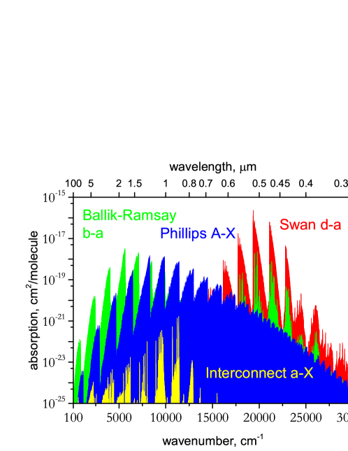
Figure 12: Electronic bands of C₂ at $T=2000$ K using a Gaussian line profile with HWHM of 5 cm^-1. The forbidden interconnection band is shown using a light (yellow) colour.

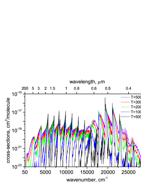
Figure 13: Temperature dependence of the C₂ cross sections using the 8states line list, from bottom to top: $T=$ 500, 1000, 2000, 3000 and 5000 K.

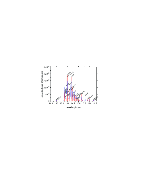
Figure 14: $X\,{}^{1}\Sigma_{g}^{+}$ – $a\,{}^{3}\Pi_{u}$ intercombination band of C₂ in absorption at $T=100$ K. Individual 8states lines and cross sections obtained using Lorentzian line profile of HWHM = 0.5 cm^-1are shown. The major features are assigned; numbers in square brackets represent the $\Omega$ spin components ${}^{3}\Pi_{\Omega}$ of the $a\,{}^{3}\Pi_{u}$ state.

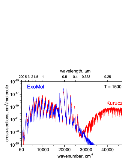
Figure 15: 8states comparing to Kurucz’s line list (Kurucz, 2011) at $T=1100$ K.

Figure 16 shows a comparison of a Swan band-head (0,0) calculated using our new line list and a stellar spectrum of V854 Cen (Kameswara Rao & Lambert, 2000). Figure 17 compares the theoretical flux spectrum of C₂ with a stellar spectrum of the Carbon star HD 92055 (Rayner et al., 2009) at the resolving power $R$=2000. Figure 18 shows a simulated Philips band (2,0) compared to the spectrum of AGB remnants of HD 56126 observed by Bakker et al. (1996). Similar spectra of this band were reported by Schmidt et al. (2013) and Ishigaki et al. (2012).

Figure 16: The C₂ Swan $(0,0)$ P branch band from the spectrum of V854 Cen on recorded on 1998 April 8 by Kameswara Rao & Lambert (2000) (lower trace), compared to the theoretical spectrum at $T$=4625 K (quoted as rotation temperature by Kameswara Rao & Lambert (2000)) using a Gaussian line profile with HWHM=0.8 cm^-1 (upper trace). The star spectrum is red-shifted by 0.2195 nm.

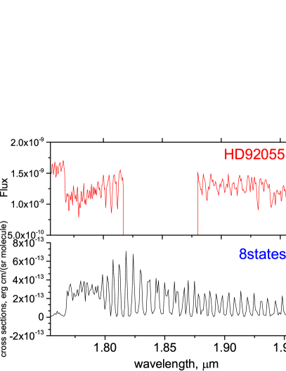
Figure 17: Swan-band: Carbon-star HD 92055 spectra observed by Rayner et al. (2009) at $R$=2000 compared to cross sections simulated using $T=5000$ K and a Gaussian profile with HWHM=1 cm^-1.

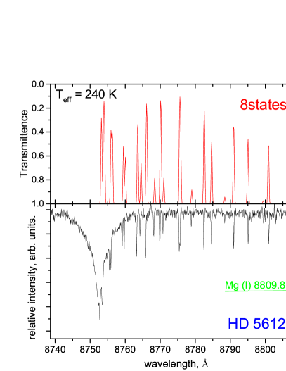
Figure 18: The Phillips band of C₂ at $T=240$ K using a Gaussian line profile with HWHM of 0.2 cm^-1 (upper display) compared to the spectrum of the AGB remnants of HD 56126 observed by Bakker et al. (1996) (lower display). The HD 56126 spectrum was shifted to match the Mg(I) line to 8809.8 Å. The theoretical transmittance spectrum is computed assuming the column amount of $10^{16}$ molecule/cm².

Figure 19 gives detailed, high resolution emission spectra of the (0,0), (1,0) and (0,1) Swan bands computed using our line list and the empirical line list by Brooke et al. (2013). Figure 20 shows a simulation of the $d$–$c$ (3,0) band of C₂ compared to the experiment by Nakajima & Endo (2014).

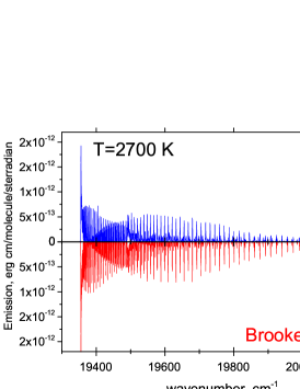
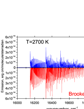
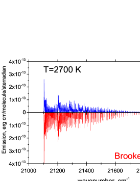
Figure 19: The C₂ Swan $(0,0)$, $(1,0)$ and $(0,1)$ bands in emission at $T=2700$ K simulated using our line list and the empirical line list of Brooke et al. (2013) and a Gaussian line profile of HWHM=0.15 cm^-1.

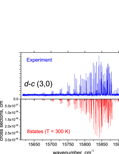
Figure 20: The $d$–$c$ band of C₂ at $T=300$ K using a Gaussian line profile with HWHM of 0.1 cm^-1 (lower display) compared to the experimental spectrum of Nakajima & Endo (2014) (upper display).

Figure 21 shows a plasma spectrum of C₂ recorded by Al-Shboul et al. (2013) compared to 8states emission cross sections at $T=$8000 K.

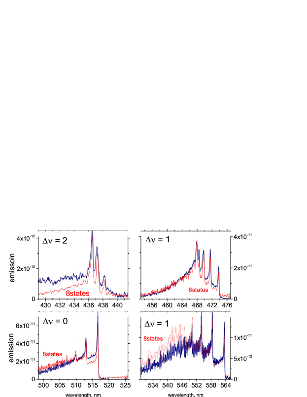
Figure 21: Swan-bands: a plasma spectrum of C₂ by Al-Shboul et al. (2013) and our emission spectrum (erg cm sr^-1molecule^-1) at $T=8000$ K for four different vibronic bands as specified in each panel. A Gaussian profile with the HWHM=4 cm^-1 was used.

5.2 Isotopic shifts

Figure 22 shows the effect of the isotopic substitution on the vibronic spectra of C₂ for the (1,0) Swan band of ¹²C₂, ¹²C¹³C and ¹³C₂ at $T=6000$ K compared to the experimental, laser-induced plasma spectrum of Dong et al. (2014).

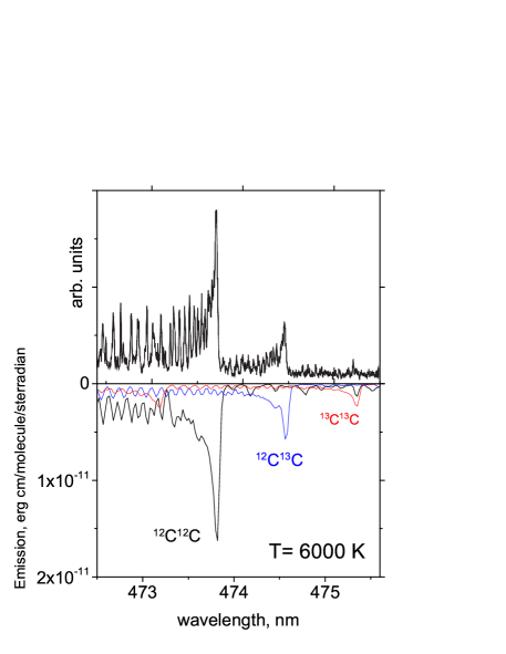
Figure 22: Isotopic shift in the spectra of C₂, Swan (1,0) for three isotopologues, ¹²C₂, ¹²C¹³C and ¹³C₂. Upper display: The experimental spectrum of a laser-induced plasma by Dong et al. (2014). Lower display: The theoretical emission spectrum at $T=$ 6000 K computed using the Gaussian profile with the HWHM=1 cm^-1 (blue-shifted by 0.1 nm to match the band heads). The theoretical abundances of ¹²C¹³C and ¹³C₂ were scaled to match the experimental intensities by the factors 0.34 and 0.14, respectively.

5.3 Partition function

As part of the line list package and as supplementary material we also report partition functions of the three C₂ isotopologues up to 10 000 K at 1 K intervals. Figure 23 shows the partition functions of ¹²C₂ computed using the 8states line list and compared to that by Sauval & Tatum (1984) and Barklem & Collet (2016). All three partition functions are in a good agreement.

We have also fitted the partition functions to the function form of Vidler & Tennyson (2000):

$$\log_{10}Q(T)=\sum\limits^{9}_{n=0}a_{n}(\log_{10}T)^{n}.$$ (13)

Table 6 gives the expansion coefficients for all three isotopologues considered, which reproduce the our partition functions within 1 % (relative values) for $T>300$ K and within $\sim$1 (absolute values) for $T<$ 300 K.

Table 6: Fitting parameters used to represent the partition functions of C₂, see Eq. (13). Fits are valid for temperatures up to 10000 K.

Parameter	12C12C	13C13C	12C13C
$a_{0}$	$7.6691867335$	$-0.0426980211$	$0.2401679500$
$a_{1}$	$-45.6411466388$	$16.5774126902$	$15.5801797784$
$a_{2}$	$91.4980228540$	$-66.5674043182$	$-65.2111429415$
$a_{3}$	$-88.7302064590$	$113.4659696600$	$112.5717888350$
$a_{4}$	$48.2113438335$	$-102.5476534740$	$-102.3357156140$
$a_{5}$	$-15.3601370784$	$54.3985236316$	$54.4790813354$
$a_{6}$	$2.8436843218$	$-17.5150320571$	$-17.5862991363$
$a_{7}$	$-0.2820217958$	$3.3710897879$	$3.3919572101$
$a_{8}$	$0.0115099797$	$-0.3570362951$	$-0.3599156561$
$a_{9}$		$0.0160186260$	$0.0161757189$

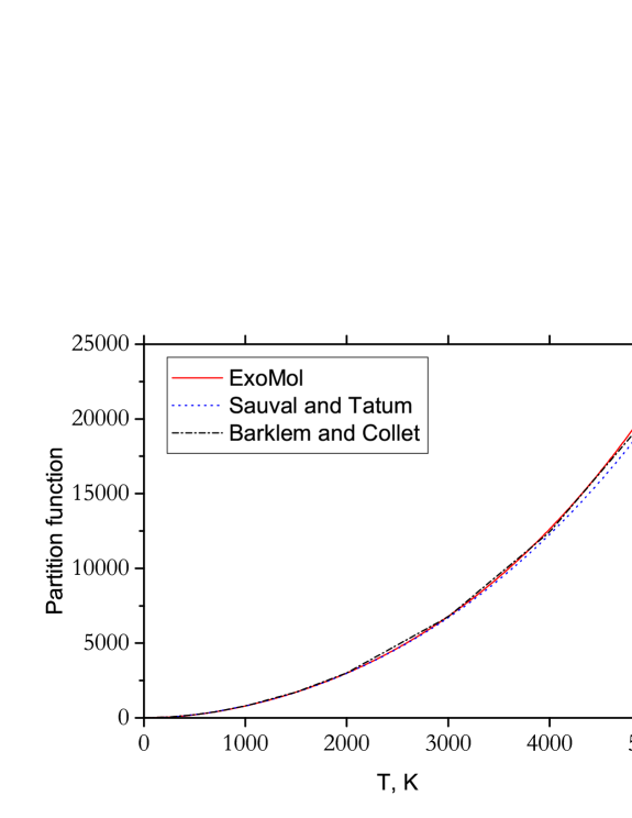
Figure 23: Temperature dependence of the partition functions of C₂ computed using our line list and compared to that by Sauval & Tatum (1984) and Barklem & Collet (2016).

5.4 Lifetime

We have computed life times of C₂ for all rovibronic states below 30 000 cm^-1. These are compared to the experimental and theoretical values by Smith (1969); Cooper & Nicholls (1975); Curtis et al. (1976); Bauer et al. (1985); Bauer et al. (1986); Naulin et al. (1988) and Erman & Iwame (1995). The agreement is good and comparable to the previous ab initio values (Davidson corrected MRCI/aug-ccpV6Z level) obtained by Schmidt & Bacskay (2007) and Kokkin et al. (2007). The lifetimes are also illustrated in Fig. 24. The rather unusual long life times of the lower rovibronic states of $a\,{}^{3}\Pi_{u}$ are explained by crossing with the lower states of $X\,{}^{1}\Sigma_{g}^{+}$ at about $J=50$, where the $a\,{}^{3}\Pi_{u}$ rovibronic states are lower than the $X\,{}^{1}\Sigma_{g}^{+}$ rovibronic states. Up to $J=48$ the lowest state in each $J$-manifold is $X\,{}^{1}\Sigma_{g}^{+}$, $v=0$, which has an infinite lifetime. Starting from $J=50$ the lowest rovibronic state with the infinite lifetime is $a\,{}^{3}\Pi_{u}$, $v=0$, $|\Omega|=1$. By $J=125$ there are six infinitively living $a\,{}^{3}\Pi_{u}$ rovibronic states ($v=0,1$).

Table 7: Experimental and calculated lifetimes of C₂ vibronic states: note the different time scales used to represent the lifetimes associated with different electronic states. Previous calculations have only considered limited decay routes for each state; these are noted in the footnote. The results suggest that these assumptions were justified.

State (units)/$v$		0	1	2	3	4	5	Source
$A\,{}^{1}\Pi_{u}$	Calc.b	$13$	$10.4$	$8.77$	$7.65$	$6.84$	$6.22$	Schmidt & Bacskay (2007)
(ms)	Calc.b	$16.6$	$13.1$	$11.0$	$9.55$	$8.50$	$7.71$	Kokkin et al. (2007)
	Exp.				$6.8\pm 2.0$	$7.1\pm 1.1$		Erman & Iwame (1995)
	Exp.	$13.4\pm 2.5$	$15.4\pm 4.0$	$14.4\pm 2.0$	$12.0\pm 2.0$	$10.7\pm 2.0$	$7.9\pm 2.0$	Bauer et al. (1985)
	Exp.	$18.5\pm 3$			$11.4\pm 2$			Bauer et al. (1986)
	Calc.	$13.13$	$10.62$	$8.95$	$7.77$	$6.93$	$6.911$	This work
$d\,{}^{3}\Pi_{g}$	Calc.c	$95.1$	$96.7$	$99.1$	$102$	$107$	$113$	Schmidt & Bacskay (2007)
(ns)	Calc.c	$98$	$99.8$	$102.4$	$106$	$110.9$	$118.2$	Brooke et al. (2013)
	Calc.c	$103.20$	$104.97$	$107.86$	$111.66$	$116.77$	$123.23$	Kokkin et al. (2007)
	Exp.	$101.8\pm 4.$	$96.7\pm 5.2$	$104\pm 17$				Naulin et al. (1988)
	Exp.	$106\pm 15$	$105\pm 15$					Bauer et al. (1986)
	Exp.	$123\pm 6$	$124\pm 6$	$130\pm 6$	$128\pm 6$	$131\pm 6$	$137\pm 10$	Curtis et al. (1976)
	Calc.	$99.37$	$101.62$	$104.71$	$108.69$	$115.18$	$119.3$	This work
$b\,^{3}\Sigma_{g}^{-}$	Calc.d	$17.83$	$14.59$	$12.47$	$11.09$	$9.88$	$9.38$	Schmidt & Bacskay (2007)
(ms)	Exp.e	$17.2$						Cooper & Nicholls (1975)
	Calc.	$17.00$	$14.46$	$12.68$	$11.46$	$10.39$	$9.612$	This work

a $D\,{}^{1}\Sigma_{u}^{+}$ $\rightarrow$ $X\,{}^{1}\Sigma_{g}^{+}$, $B^{\prime}\,{}^{1}\Sigma_{g}^{+}$ and $C\,{}^{1}\Pi_{g}$ only considered.

b $A\,{}^{1}\Pi_{u}$ $\rightarrow$ $X\,{}^{1}\Sigma_{g}^{+}$ only considered.

c $d\,{}^{3}\Pi_{g}$ $\rightarrow$ $a\,{}^{3}\Pi_{u}$ only considered.

d $b\,^{3}\Sigma_{g}^{-}$ $\rightarrow$ $a\,{}^{3}\Pi_{u}$ only considered.

e Average value for a range of vibrational states

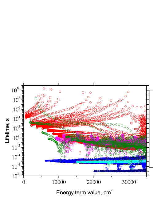
Figure 24: Lifetimes of rovibronic states of C₂. The black solid squares representing the $A\,{}^{1}\Pi_{u}$ state values are hidden behind the blue open triangles of the $b\,^{3}\Sigma_{g}^{-}$ state.

6 Conclusions

New empirical rovibronic line lists for three isotopologues of C₂ (¹²C₂,¹³C₂ and ¹²C¹³C) are presented. These line lists, called 8states, are based on high level ab initio (MRCI) calculations and empirical refinement to the experimentally derived energies of ¹²C₂. The line lists cover eight lowest electronic (singlet and triplet) states $X\,{}^{1}\Sigma_{g}^{+}$, $A\,{}^{1}\Pi_{u}$, $B\,{}^{1}\Delta_{g}$, $B^{\prime}\,{}^{1}\Sigma_{g}^{+}$, $a\,{}^{3}\Pi_{u}$, $b\,^{3}\Sigma_{g}^{-}$, $c\,^{3}\Sigma_{u}^{+}$  and $d\,{}^{3}\Pi_{g}$ fully coupled in the nuclear motion calculations through spin-orbit and electronic angular momentum curves and complemented by empirical curves representing different corrections (Born-Oppenheimer-breakdown, $\Lambda$-doubling, spin-spin and spin-rotation). The line lists should be complete up to about 30 000 cm^-1 with the energies stretching up to 50 000 cm^-1. In order to improve the accuracy of the line positions, where available the empirical energies were replaced by experimentally derived MARVEL values. The line lists were benchmarked against high temperature stellar and plasma spectra. Experimental lifetimes were especially important for assessing our absolute intensities as well as the quality of the underlined ab initio dipole moments of C₂ used. The line lists, the spectroscopic models and the partition functions are available from the CDS (http://cdsarc.u-strasbg.fr) and ExoMol (www.exomol.com) databases.

7 Acknowledgements

We thank Andrey Stolyarov, Timothy W. Schmidt and George B. Bacskay for help at different stages of the project. This work was supported by the UK Science and Technology Research Council (STFC) No. ST/M001334/1 and the COST action MOLIM No. CM1405. This work made extensive use of UCL’s Legion high performance computing facility. A part of the calculations were performed using DARWIN, high performance computing facilities provided by DiRAC for particle physics, astrophysics and cosmology and supported by BIS National E-infrastructure capital grant ST/J005673/1 and STFC grants ST/H008586/1, ST/K00333X/1.

References

- Abrams & Sherrill (2004) Abrams M., Sherrill C., 2004, J. Chem. Phys., 121, 9211
- Al-Shboul et al. (2013) Al-Shboul K. F., Harilal S. S., Hassanein A., 2013, J. Appl. Phys., 113, 163305
- Amiot (1983) Amiot C., 1983, ApJS, 52, 329
- Amiot et al. (1979) Amiot C., Chauville J., Mailllard J.-P., 1979, J. Mol. Spectrosc., 75, 19
- Bakker et al. (1996) Bakker E. J., Waters L. B. F. M., Lamers H. J. G. L. M., Trams N. R., van der Wolf F. L. A., 1996, A&A, 310, 893
- Ballik & Ramsay (1963) Ballik E. A., Ramsay D. A., 1963, ApJ, 137, 84
- Barklem & Collet (2016) Barklem P. S., Collet R., 2016, A&A, 588, A96
- Bauer et al. (1985) Bauer W., Becker K. H., Hubrich C., Meuser R., Wildt J., 1985, ApJ, 296, 758
- Bauer et al. (1986) Bauer W., Becker K. H., Bielefeld M., Meuser R., 1986, Chem. Phys. Lett., 123, 33
- Bauer et al. (2017) Bauer W., Fox C., Gosse R., Perram G., 2017, Opt. Eng., 56
- Bernath (2005) Bernath P. F., 2005, Spectra of Atoms and Molecules, 2nd edn. Oxford University Press
- Black & van Dishoeck (1988) Black J. H., van Dishoeck E. F., 1988, ApJ, 331, 986
- Bornhauser et al. (2011) Bornhauser P., Sych Y., Knopp G., Gerber T., Radi P. P., 2011, J. Chem. Phys., 134, 044302
- Bornhauser et al. (2013) Bornhauser P., Sych Y., Knopp G., Gerber T., Radi P. P., 2013, Chem. Phys. Lett., 572, 16
- Bornhauser et al. (2015) Bornhauser P., Marquardt R., Gourlaouen C., Knopp G., Beck M., Gerber T., van Bokhoven J. A., Radi P. P., 2015, J. Chem. Phys., 142, 094313
- Brault et al. (1982) Brault J. W., Delbouille L., Grevesse N., Roland G., Sauval A. J., Testerman L., 1982, A&A, 108, 201
- Brockhinke et al. (1998) Brockhinke A., Hartlieb A. T., Kohse-Hoinghaus K., Crosley D. R., 1998, Appl. Phys. B, 67, 659
- Brooke et al. (2013) Brooke J. S., Bernath P. F., Schmidt T. W., Bacskay G. B., 2013, J. Quant. Spectrosc. Radiat. Transf., 124, 11
- Brown & Merer (1979) Brown J. M., Merer A. J., 1979, J. Mol. Spectrosc., 74, 488
- Brown et al. (1975) Brown J. M., et al., 1975, J. Mol. Spectrosc., 55, 500
- Bunker & Jensen (1998) Bunker P. R., Jensen P., 1998, Molecular Symmetry and Spectroscopy, 2 edn. NRC Research Press, Ottawa
- Bunker et al. (1997) Bunker P. R., Schutte C. J. H., Hougen J. T., Mills I. M., Watson J. K. G., Winnewisser B. P., 1997, Pure Appl. Chem., 69, 1651
- Chaffee & Lutz (1978) Chaffee Jr. F.-H., Lutz B.-L., 1978, ApJL, 221, L91
- Chaffee et al. (1980) Chaffee F. H., Lutz B. L., Black J. H., Vandenbout P. A., Snell R. L., 1980, ApJ, 236, 474
- Chan et al. (2004) Chan M.-C., Yeung S.-H., Wong Y.-Y., Li Y., Chan W.-M., Yim K.-H., 2004, Chem. Phys. Lett., 390, 340
- Chan et al. (2013) Chan M.-C., Yeung S.-H., Wang N., Cheung A. S.-C., 2013, J. Phys. Chem. A, 117, 9578
- Chauville et al. (1977) Chauville J., Maillard J. P., Mantz A. W., 1977, J. Mol. Spectrosc., 68, 399
- Chen et al. (2015) Chen W., Kawaguchi K., Bernath P. F., Tang J., 2015, J. Chem. Phys., 142, 064317
- Chen et al. (2016) Chen W., Kawaguchi K., Bernath P. F., Tang J., 2016, J. Chem. Phys., 144, 064301
- Cooper & Nicholls (1975) Cooper D. M., Nicholls R. W., 1975, J. Quant. Spectrosc. Radiat. Transf., 15, 139
- Curtis & Sarre (1985) Curtis M. C., Sarre P. J., 1985, J. Mol. Spectrosc., 114, 427
- Curtis et al. (1976) Curtis L., Engman B., Erman P., 1976, Phys. Scr., 13, 270
- Danks et al. (1974) Danks A. C., Lambert D. I., Arpigny C., 1974, ApJ, 194, 745
- Davis et al. (1988a) Davis S. P., Abrams M. C., Sandalphon Brault J. W., Rao M. L. P., 1988a, J. Opt. Soc. Am. B, 5, 1838
- Davis et al. (1988b) Davis S. P., Abrams M. C., Phillips J. G., Rao M. L. P., 1988b, J. Opt. Soc. Am. B, 5, 2280
- De Mello et al. (2009) De Mello A. B., Lorenz-Martins S., de Araújo F. X., Pereira C. B., Landaberry S. J. C., 2009, ApJ, 705, 1298
- Dong et al. (2014) Dong M., Chan G. C.-Y., Mao X., Gonzalez J. J., Lu J., Russo R. E., 2014, Spectra Chimica Acta B, 100, 62
- Douay et al. (1988a) Douay M., Nietmann R., Bernath P. F., 1988a, J. Mol. Spectrosc., 131, 250
- Douay et al. (1988b) Douay M., Nietmann R., Bernath P. F., 1988b, J. Mol. Spectrosc., 131, 261
- Dunning (1989) Dunning T. H., 1989, J. Chem. Phys., 90, 1007
- Erman & Iwame (1995) Erman P., Iwame A., 1995, ApJ, 450, L31
- Federman & Huntress (1989) Federman S. R., Huntress Jr. W. T., 1989, ApJ, 338, 140
- Feller & Sordo (2000) Feller D., Sordo J. A., 2000, J. Chem. Phys., 113, 485
- Freymark (1951) Freymark H., 1951, Annalan der Physik, 8, 221
- Fujita (1980) Fujita Y., 1980, Space Sci. Rev., 25, 89
- Furtenbacher et al. (2016) Furtenbacher T., Szabó I., Császár A. G., Bernath P. F., Yurchenko S. N., Tennyson J., 2016, ApJS, 224, 44
- Gamache et al. (2017) Gamache R. R., et al., 2017, J. Quant. Spectrosc. Radiat. Transf., 203, 70
- Gonneau, A. et al. (2017) Gonneau, A. et al., 2017, A&A, 601, A141
- Goorvitch (1990) Goorvitch D., 1990, ApJS, 74, 769
- Goorvitch (1990) Goorvitch D., 1990, ApJS, 74, 769
- Gredel et al. (1989) Gredel R., van Dishoeck E. F., Black J. H., 1989, ApJ, 338, 1047
- Green (2013) Green P., 2013, ApJ, 765, 12
- Grevesse & Sauval (1973) Grevesse N., Sauval A. J., 1973, A&A, 27, 29
- Hall & Maxwell (2008) Hall P. B., Maxwell A. J., 2008, ApJ, 678, 1292
- Hardwick & Winicur (1986) Hardwick J. L., Winicur D. H., 1986, J. Mol. Spectrosc., 115, 175
- Hobbs (1979) Hobbs L. M., 1979, ApJL, 232, L175
- Hobbs (1981) Hobbs L. M., 1981, ApJ, 243, 485
- Hobbs & Campbell (1982) Hobbs L. M., Campbell B., 1982, ApJ, 254, 108
- Hobbs et al. (1983) Hobbs L. M., Black J. H., van Dishoeck E. F., 1983, ApJ, 271, L95
- Hornkohl et al. (2011) Hornkohl J. O., Nemes L., Parigger C., 2011, Spectroscopy, Dynamics and Molecular Theory of Carbon Plasmas and Vapors (Eds. L. Nemes and S. Irle). World Scientific
- Hupe et al. (2012) Hupe R. C., Sheffer Y., Federman S. R., 2012, ApJ, 761, 38
- Ishigaki et al. (2012) Ishigaki M. N., Parthasarathy M., Reddy B. E., García-Lario P., Takeda Y., Aoki W., García-Hernández D. A., Manchado A., 2012, MNRAS, 425, 997
- Joester et al. (2007) Joester J. A., Nakajima M., Reilly N. J., Kokkin D. L., Nauta K., Kable S. H., Schmidt T. W., 2007, J. Chem. Phys., 127, 214303
- Johnson et al. (1983) Johnson J. R., Fink U., Larson H. P., 1983, ApJ, 270, 769
- Jönsson et al. (2007) Jönsson M., Nerushev O. A., Campbell E. E. B., 2007, Appl. Phys. A, 88, 261
- Kameswara Rao & Lambert (2000) Kameswara Rao N., Lambert D. L., 2000, MNRAS, 313, L33
- Kaniki et al. (2003) Kaniki J., Yang X. H., Guo Y. C., Yu S. S., Li B. X., Liu Y. Y., Chen Y. Q., 2003, Prog. Nat. Sci., 13, 736
- Keenan (1993) Keenan P. C., 1993, PASP, 105, 905
- Keenan & Morgan (1941) Keenan P. C., Morgan W. W., 1941, ApJ, 94, 501
- Kokkin et al. (2007) Kokkin D. L., Bacskay G. B., Schmidt T. W., 2007, J. Chem. Phys., 126, 084302
- Krechkivska et al. (2015) Krechkivska O., Bacskay G. B., Troy T. P., Nauta K., Kreuscher T. D., Kable S. H., Schmidt T. W., 2015, J. Phys. Chem. A, 119, 12102
- Kurucz (2011) Kurucz R. L., 2011, Can. J. Phys., 89, 417
- Lambert (1968) Lambert D. L., 1968, MNRAS, 138, 143
- Lambert (1978) Lambert D. L., 1978, MNRAS, 182, 249
- Lambert & Danks (1983) Lambert D. L., Danks A. C., 1983, ApJ, 268, 428
- Lambert et al. (1984) Lambert D. L., Brown J. A., Hinkle K. H., Johnson H. R., 1984, ApJ, 284, 223
- Le Roy (2017) Le Roy R. J., 2017, J. Quant. Spectrosc. Radiat. Transf., 186, 167
- Lebourlot & Roueff (1986) Lebourlot J., Roueff E., 1986, J. Mol. Spectrosc., 120, 157
- Lee et al. (1999) Lee E. G., Seto J. Y., Hirao T., Bernath P. F., Le Roy R. J., 1999, J. Mol. Spectrosc., 194, 197
- Lloyd & Ewart (1999) Lloyd G. M., Ewart P., 1999, J. Chem. Phys., 110, 385
- Lodi et al. (2015) Lodi L., Yurchenko S. N., Tennyson J., 2015, Mol. Phys., 113, 1559
- Martin (1992) Martin M., 1992, J. Photochem. Photobiol. A, 66, 263
- Mayer & O’dell (1968) Mayer P., O’dell C. R., 1968, ApJ, 153, 951
- McKemmish et al. (2016) McKemmish L. K., Yurchenko S. N., Tennyson J., 2016, MNRAS, 463, 771
- Medvedev et al. (2016) Medvedev E. S., Meshkov V. V., Stolyarov A. V., Ushakov V. G., Gordon I. E., 2016, J. Mol. Spectrosc., 330, 36
- Meunier (1911) Meunier J., 1911, C R Hebd Seances Acad Sci, 153, 863
- Nakajima & Endo (2014) Nakajima M., Endo Y., 2014, J. Mol. Spectrosc., 302, 9
- Nakajima & Endo (2013) Nakajima M., Endo Y., 2013, J. Chem. Phys., 139, 244310
- Naulin et al. (1988) Naulin C., Costes M., Dorthe G., 1988, Chem. Phys. Lett., 143, 496
- Newburn & Spinrad (1984) Newburn R., Spinrad H., 1984, AJ., 89, 289
- Owen (1973) Owen T., 1973, ApJ, 184, 33+
- Patrascu et al. (2014) Patrascu A. T., Hill C., Tennyson J., Yurchenko S. N., 2014, J. Chem. Phys., 141, 144312
- Patrascu et al. (2015) Patrascu A. T., Tennyson J., Yurchenko S. N., 2015, MNRAS, 449, 3613
- Peterson & Dunning (2002) Peterson K. A., Dunning T. H., 2002, J. Chem. Phys., 117, 10548
- Petrova & Sinitsa (2006) Petrova T., Sinitsa L., 2006, Opt. Spectrosc., 101, 871
- Phillips (1948a) Phillips J. G., 1948a, ApJ, 107, 387
- Phillips (1948b) Phillips J. G., 1948b, ApJ, 110, 73
- Prajapat et al. (2017) Prajapat L., Jagoda P., Lodi L., Gorman M. N., Yurchenko S. N., Tennyson J., 2017, MNRAS, 472, 3648
- Prasad & Bernath (1994) Prasad C. V. V., Bernath P. F., 1994, ApJ, 426, 812
- Querci et al. (1971) Querci F., Querci M., Kunde V. G., 1971, A&A, 15, 256
- Rayner et al. (2009) Rayner J. T., Cushing M. C., Vacca W. D., 2009, ApJS, 185, 289
- Roos & Taylor (1980) Roos B. O., Taylor P. R., 1980, Chem. Phys., 48, 157
- Rousselot et al. (1995) Rousselot P., Moreels G., Clairemidi J., Goidetdevel B., Boehnhardt H., 1995, Icarus, 114, 341
- Rousselot et al. (2012) Rousselot P., Jehin E., Manfroid J., Hutsemékers D., 2012, A&A, 545, A24
- Rousselot et al. (1998) Rousselot P., Laffont C., Moreels G., Clairemidi J., 1998, A&A, 335, 765
- Roux et al. (1985) Roux F., Wannous G., Michaud F., Verges J., 1985, J. Mol. Spectrosc., 109, 334
- Sauval & Tatum (1984) Sauval A. J., Tatum J. B., 1984, ApJS, 56, 193
- Schmidt & Bacskay (2007) Schmidt T. W., Bacskay G. B., 2007, J. Chem. Phys., 127, 234310
- Schmidt et al. (2013) Schmidt M. R., Začs L., Pułecka M., Szczerba R., 2013, A&A, 556, A46
- Sherrill & Piecuch (2005) Sherrill C., Piecuch P., 2005, J. Chem. Phys., 122, 124104
- Smith (1969) Smith W. H., 1969, ApJ, 156, 791
- Snow & McCall (2006) Snow T. P., McCall B. J., 2006, ARA&A, 44, 367
- Sonnentrucker et al. (2007) Sonnentrucker P., Welty D. E., Thorburn J. A., York D. G., 2007, ApJS, 168, 58
- Sorkhabi et al. (1997) Sorkhabi O., Blunt V. M., Lin H., Xu D., Wrobel J., Price R., Jackson W. M., 1997, J. Chem. Phys., 107, 9842
- Souza & Lutz (1977) Souza S. P., Lutz B. L., 1977, ApJ, 216, L49