Water and OH Emission from the inner disk of a Herbig Ae/Be star

Abstract

We report the detection of hot H₂O and OH emission from the Herbig Ae/Be star HD 101412 using the Cryogenic Infrared Echelle Spectrograph on the Very Large Telescope. Previous studies of Herbig Ae/Be stars have shown the presence of OH around some of these sources, but H₂O has proven more elusive. While marginal water emission has been reported in the mid-infrared, and a few Herbig Ae/Be stars show water emission in the far-infrared, water emission near 2.9 $\mu$m has not been previously detected. We apply slab models to the ro-vibrational OH, H₂O, and CO spectra of this source and show that the molecules are consistent with being cospatial. We discuss the possibility that the detection of the CO overtone bandhead emission, detection of water emission, and the large line to continuum contrast of the OH lines may be connected to its high inclination and the $\lambda$ Boö nature of this star. If the low abundance of refractories results from the selective accretion of gas relative to dust, the inner disk of HD 101412 should be strongly dust-depleted allowing us to probe deeper columns of molecular gas in the disk, enhancing its molecular emission. Our detection of C- and O-bearing molecules from the inner disk of HD 101412 is consistent with the expected presence in this scenario of abundant volatiles in the accreting gas.

1. Introduction

High resolution spectroscopic studies of Herbig Ae/Be (HAeBe) stars indicate that their circumstellar environments are commonly home to hot CO (Blake & Boogert, 2004; Brittain et al., 2007; Salyk et al., 2011b, a; Brown et al., 2013; van der Plas et al., 2015; Banzatti & Pontoppidan, 2015) and, less frequently, OH gas (Mandell et al., 2008; Fedele et al., 2011; Brittain et al., 2016), but they have yet to yield a detection of the H₂O emission from 2-4 $\mu$m that has been observed in lower-mass pre-main sequence T Tauri systems (Carr et al., 2004; Salyk et al., 2008; Fedele et al., 2011; Doppmann et al., 2011; Mandell et al., 2012; Banzatti et al., 2017).

Likewise, mid- and far-infrared studies have yielded few detections of H₂O emission from cooler gas in disks around HAeBes. In a study of 25 HAeBes using Spitzer, there were marginal detections of H₂O emission reported for 12 of 25 systems (Pontoppidan et al., 2010). These detections were reported based on inspection by eye and were not determined to be above the 3.5$\sigma$ detection threshold defined in the study. In contrast, similar surveys of T Tauri stars yield a much higher detection rate for H₂O emission in the mid-infrared (22 of 48 exhibited a significant detection of H₂O emission; Pontoppidan et al. 2010). Statistics compiled by Banzatti et al. (2017) showed that between 63-85 % out of 64 stars with a stellar mass less than 1.5 M_⊙ exhibit mid-infrared H₂O emission. In searches for H₂O in the far-infrared, only 3 sources were detected out of 25 HAeBes observed (Meeus et al., 2012; Fedele et al., 2012, 2013). These results suggests that the abundance of H₂O gas in the optically thin upper atmosphere around HAeBes is low.

One possible explanation for the dearth of near-infrared (NIR) water detections among HAeBes compared to T Tauri stars is that the high far-ultraviolet (FUV) luminosity of HAeBe stars causes a larger column of water to be dissociated to produce OH (e.g., Ádámkovics et al. 2016; Najita & Ádámkovics 2017). As the water falls below the dust photosphere, emission from the water becomes impossible to detect. Here we report what appears to be an exception to this picture - the first detection of NIR H₂O emission from the HAeBe star HD 101412.

HD 101412 is a B9.5Ve star (Valenti et al., 2003) located at a distance of 411${}^{+5}_{-4}$ pc (Gaia Collaboration et al., 2016, 2018). As part of an X-Shooter survey of 92 HAeBes, Fairlamb et al. (2015) determined the stellar parameters of their sample self-consistently. They find that T_eff = 9750 $\pm$ 250 K and log(L/L_⊙) = 1.36 $\pm$ 0.23 adopting d = 301 pc. We adopt the Gaia distance and use Siess pre-main sequence models to recalculate the stellar mass, radius, and luminosity (Siess et al., 2000). The updated values are M = 2.5 M_⊙, R = 2.3 R_⊙, and log(L/L_⊙) = 1.63.

The inner disk surrounding HD 101412 is nearly edge-on. Fitting a uniform ring model to $N-$band visibilities acquired with MIDI on the VLT indicates that the disk is inclined 80$\arcdeg$ $\pm$ 7$\arcdeg$ (Fedele et al., 2008). No (sub)mm observations have been made of this source so there is no observational estimate of the extent or mass of the disk. The mid-infrared SED of the star indicates that it is a self-shadowed disk (Group II; Fedele et al. 2008). Fairlamb et al. (2017) report the flux of H$\alpha$ for this source and provide a relationship between the accretion luminosity and luminosity of the H$\alpha$ line. Adopting the stellar parameters above, we find that the accretion rate is 1.6 $\times$ 10^-7 M_☉ yr^-1. The accretion rate indicates that HD 101412 still harbors a large gaseous reservoir.

The disk of HD 101412 reveals a rich molecular spectrum. Both the ro-vibrational CO overtone (Cowley et al., 2012; Ilee et al., 2014; van der Plas et al., 2015) and fundamental (van der Plas et al., 2015) emission lines have been observed. Modeling of the profile of these lines indicate that the emitting region is narrow (0.8 - 1.2 AU; van der Plas et al. 2015). Mid-infrared spectroscopy also reveals CO₂ emission from the disk of HD 101412 (Pontoppidan et al., 2010; Salyk et al., 2011b). CO₂ emission and CO bandheads of the first overtone emission are both unusual features to observe in the spectrum of HAeBe stars. Only 7% show CO overtone bandhead emission in a survey of 91 HAeBes (Ilee et al., 2014) and only 4% show CO₂ emission in a survey of 25 HAeBes (Salyk et al., 2011b). Here we report the detection of ro-vibrational OH and H₂O emission from this source as well (Sections 2 and 3). We apply slab models of CO, OH, and H₂O to compare the emitting radii, temperature, and column densities of these molecules (Section 4), and compare the molecular emission observed in HD 101412 to other young stellar objects (Section 5). Finally, we discuss the implications for our understanding of the molecular content of the inner disks around HAeBe stars (Section 6).

2. Observations

$L$-band observations of HD 101412 were obtained from the European Southern Observatory (ESO) Data Archives along with the associated raw calibration files, based on observations under programme ID 091.C-0796(A). The data were acquired on 27 May 2013 using a 0.^′′2 slit width at a central wavelength of 2.94 $\mu$m using the Cryogenic Infrared Echelle Spectrograph (CRIRES; Käufl et al. 2004) on the ESO Very Large Telescope (VLT) UT1. CRIRES has four detectors that each cover $\sim$0.0160 $\mu$m with a $\sim$0.0045 $\mu$m gap between each chip. Exposures were taken in an ABBA nod pattern with a 10.^′′ nod in order to remove sky emission lines. An integration time of 60 s and 3 sub-integrations were used for each of 20 exposures giving a total integration time of 3600 s. Table 1 gives details of all observations used in this study.

Table 1Observations

Star	Date	Airmass	Exposures	Int. Time (s)
$L-$Band
HD 101412	20130527	1.265	20	3600
$\lambda$ Cen	20130527	1.277	8	240
$K-$Band
HD 101412	20110405	1.250	8	4800
j Cen	20110405	1.301	8	640

Note. — Observation information for HD 101412 OH, H₂O, and CO data presented. All data were obtained using the ESO Data Archives.

Data reduction was performed using software based on algorithms developed for the reduction of PHOENIX and NIRSPEC data (described in Brittain et al. 2007). Flats and darks were taken in order to remove systematic variation in pixel gain. Sequential AB observations were combined (A - B) and then divided by the normalized flat field image. Median values of the combined images were used to identify and remove hot and bad pixels, as well as cosmic ray hits. Pixel values that differ by 6$\sigma$ were rejected. Spectra were then extracted using a rectangular extraction method. Wavelength calibration was performed using the telluric absorption features observed in the spectrum. A Sky Synthesis Program (SSP) model atmosphere (Kunde & Maguire, 1974), which accesses the 2003 HITRAN molecular database (Rothman et al., 2003), was computed based on the airmass of the observations. Standard star observations of $\lambda$ Cen were taken immediately after the observations of HD 101412. The telluric standard was reduced following the same process as HD 101412. The normalized spectrum of HD 101412 was divided by the normalized spectrum of $\lambda$ Cen to correct for atmospheric absorption lines. Regions of the spectrum where the atmospheric transmittance was below 50% were excluded. Final reduced $L-$band spectra and ratios are presented in Figure 1.

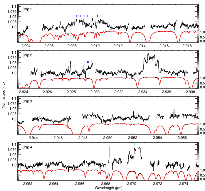
Figure 1.— $L-$band observations of HD 101412. Chip 1 is the upper plot and chip 4 is the lower plot, with the gap between each plot resulting from the gaps between the chips. In each panel we plot the normalized spectrum of HD 101412 (black) and the telluric standard $\lambda$ Cen (HR 4467) (red). The telluric corrected spectrum of HD 101412 is plotted above (stretched by a factor of 20 and offset by 0.5 units). The left axis shows the normalized flux units scaled to the ratioed spectrum while the right axis shows the normalized flux units for the science and standard star spectra. The locations of the OH emission doublets are marked with green hashes with the structure observed in the continuum coming from H₂O emission, with the strongest H₂O features marked with blue hashes.

We also reduced archival data for the CO bandhead emission previously reported for HD 101412 (Cowley et al., 2012; Ilee et al., 2014). The data were obtained based on observations made with CRIRES on the VLT under programme ID 087.C-0124(A). The CO data were re-reduced using the same method as the OH and H₂O observations. The CO data were then modeled in order to self-consistently determine the CO emitting region, temperature, and column density.

The flux densities adopted for the continua of the $K$- and $L$-band spectra were obtained using values from Johnson:K and Johnson:L filter photometry measurements found using the VizieR Photometry Viewer (Ochsenbein et al., 2000). The flux density at 2.94 $\mu$m was estimated at a value between the flux density at these filters by a linear fit to the two data points. A continuum flux of 3.20 $\times$ 10^-10 erg s^-1 cm^-2 $\mu$m^-1 was used for the $L$-band (OH) and 4.21 $\times$ 10^-10 erg s^-1 cm^-2 $\mu$m^-1 was used for the $K$-band (CO).

3. Results

The fully reduced $L-$band spectrum has a spectral resolution of R $\approx$ 90,000 and a signal to noise ratio of $\sim$200. We detect the OH P4.5 and OH P5.5 doublets with the peak in the normalized line flux relative to the continuum of 9% (Figure 2, panel A and C, respectively). Gaps in the profile of the P5.5 doublet are due to telluric absorption greater than 50%. We also detect H₂O emission near 2.93 $\mu$m (Figure 4). Another H₂O feature between 2.9074 and 2.9110 $\mu$m is also observed (Figure 5). Table 2 gives transition parameters for the individual transitions that we propose comprise the most prominent emission features. Errors for equivalent widths are determined by adding the noise across each pixel in the emission feature in quadrature.

Table 2Molecular Line Properties

Wavelength	Transition	Aul	gu	Eu
($\mu$m)		(s-1)		(K)
OH Lines
2.97040	3/2 P5.5f	12.67	20	5627.64
2.96997	3/2 P5.5e	12.67	20	5626.56
2.93461	3/2 P4.5f	11.68	16	5414.92
2.93428	3/2 P4.5e	11.68	16	5414.31
H2O Lines
2.92949	10 8 2 $\rightarrow$ 11 8 3	18.45	63	8540.39
2.92948	10 8 3 $\rightarrow$ 11 8 4	21.20	21	8540.39
2.92925	11 5 6 $\rightarrow$ 12 5 7	39.56	23	8221.99
2.92924	14 2 13 $\rightarrow$ 15 2 14	48.79	29	8697.67
2.92920	14 1 13 $\rightarrow$ 15 1 14	48.58	87	8697.71
2.92912	13 3 11 $\rightarrow$ 14 3 12	48.45	81	8583.04
2.92909	13 2 11 $\rightarrow$ 14 2 12	48.94	27	8582.23
2.91011	13 2 12 $\rightarrow$ 14 2 13	48.78	81	8293.46
2.91011	13 1 11 $\rightarrow$ 14 1 12	48.91	27	8293.43
2.90998	12 2 10 $\rightarrow$ 13 2 11	49.17	75	8177.10
2.90997	12 3 10 $\rightarrow$ 13 3 11	48.16	25	8178.82
2.90911	10 6 4 $\rightarrow$ 11 6 5	31.81	63	8030.62
2.90886	11 3 8 $\rightarrow$ 12 3 9	53.09	23	7976.11
2.90848	10 6 5 $\rightarrow$ 11 6 6	31.57	21	8029.60
2.90829	11 4 8 $\rightarrow$ 12 4 9	42.70	69	8004.54
2.90817	14 1 14 $\rightarrow$ 15 1 15	48.52	29	8340.48
2.90813	14 0 14 $\rightarrow$ 15 0 15	48.04	81	8340.56

Note. — Parameters for some transitions that comprise observed emission features in HD 101412 $L-$band observations. Line groups are presented in the order that the emission feature is discussed in the text. All data were acquired using the HITRAN database (Rothman et al., 2013).

3.1. OH Emission

The P4.5 doublet transition is spectrally resolved, however, the doublet itself is blended. The emission feature is bracketed by strong telluric absorption features. The equivalent width (EW) is calculated over the entire range of the doublet between the absorption features and divided by 2 due to the blending. The EW is 4.3 $\pm$ 0.2 $\times$ 10^-5 $\mu$m which, when factoring in the distance and $L$-band flux density, corresponds to a line luminosity of 7.2 $\pm$ 0.3 $\times$ 10^-5 L_⊙. The line to continuum contrast of the P4.5 OH doublet is 9% (Figure 2) which is more than three times the line to continuum contrast typically observed for this doublet in previous observations of HAeBes (Mandell et al., 2008; Fedele et al., 2011; Brittain et al., 2016).

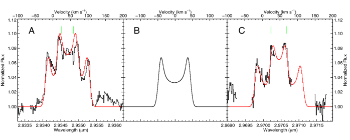
Figure 2.— (A) P4.5 (1+, 1$-$) OH emission doublet. The normalized fluxes of the OH doublets are plotted versus wavelength. The upper x-axis shows the relative velocity of the emission features. Zero velocity is centered at the laboratory rest wavelength of the P4.5 (1+) line (2.93428 $\mu$m). The green tick marks indicate the wavelength of each doublet feature in the rest frame of the star. The Doppler shift inferred from the molecular emission indicates that the heliocentric radial velocity is 16.9 km s^-1, which is consistent with the heliocentric radial velocity inferred from the measurement of photospheric lines (16.5 km s^-1; Hubrig et al. 2010). The best fit model is plotted in red. (B) Model line profile of each doublet feature, scaled to match P4.5 intensity. (C) P5.5 (1+, 1$-$) OH emission feature. The emission feature is partially obscured by telluric absorption. The green tick marks indicate the location of each doublet feature in the rest frame of the star. The zero velocity bin is centered at 2.96997 $\mu$m, which is the laboratory rest wavelength of the P5.5 (1+) lines.

The P5.5 emission feature is partially obscured by atmospheric absorption. The profile of the P5.5 doublet and P4.5 doublet differ slightly in the blue portion due to different separations of the doublet transition energies. Thus, the individual peaks in the blue portion of the P5.5 feature show each doublet’s peak as being further apart. This broadens the overall line width, however, the inner peak separation between the blue portion of the (1$-$) line and red portion of the (1+) line is reduced. Due to the atmospheric absorption, an EW cannot be determined from the data. Based on the model fits obtained from fitting the full P4.5 doublet, we determine the P5.5 EW to be 3.7 $\pm$ 0.1 $\times$ 10^-5 $\mu$m which corresponds to a line luminosity of 6.2 $\pm$ 0.3 $\times$ 10^-5 L_⊙.

We observe a Doppler shift of 24.4 km s^-1. This implies a heliocentric radial velocity of 16.9 km s^-1 based on the date the observations were made. Hubrig et al. (2010) observe Fe lines in the spectrum of HD 101412 and report an average heliocentric radial velocity of 16.65 km s^-1, which is consistent with our determined radial velocity.

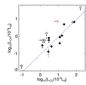
Figure 3.— Adapted from Brittain et al. (2016). HD 101412 has been added and is plotted in red. Group I HAeBe stars are marked as filled symbols. Group II HAeBe stars are marked as open symbols. The disks that have been observed to have an optically thin inner disk are labeled with “plus” signs. Disks without such optically thin regions are labeled with diamonds. The dotted-dashed line is a linear least-squares fit to the detections, not including HD 101412.

Brittain et al. (2016) find a power-law relationship between the luminosity of ro-vibrational CO ($\nu$ = 1 $\rightarrow$ 0 P30) and OH ($\nu$ = 1 $\rightarrow$ 0 P4.5) emission from HAeBes and find that the ratio of their luminosities is 11.0$\pm$0.2. We compare the relative luminosity of the OH and CO emission for HD 101412 (Figure 3). Because the lines are so broad, there is significant line blending. We take the most isolated CO line ($\nu$ = 1 $\rightarrow$ 0 P26 transition; Troutman 2010) and determine the luminosity of the P30 line assuming the gas is 1300 K (see section 4). Because of the line blending, we take the CO luminosity to be an upper limit and find that L(CO)/L(OH) $\leq$ 1.24. Thus the relative flux of the OH emission is an order of magnitude larger than the previous HAeBes studied.

3.2. H₂O Emission

One prominent H₂O emission feature is observed at 2.929 $\mu$m (Figure 4). This feature is partially obscured by telluric absorption. The emission is due to a blend of multiple transitions. Table 2 presents some transitions that comprise the emission feature.

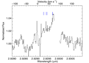
Figure 4.— The 2.93 $\mu$m H₂O emission lines. The blue tick marks indicate the positions of the dominant transitions contributing to the emission feature. The zero velocity bin is centered at 2.92909 $\mu$m, the transition with the shortest wavelength of the list in Table 2 found in this spectral region. The upper x-axis gives the velocity space information and shows a Doppler shift of 24.4 km s^-1, consistent with the OH lines.

Another H₂O emission feature is observed between 2.9074 and 2.9110 $\mu$m (Figure 5), with some regions obscured by atmospheric absorption. This feature is also a blend of multiple transitions. In both instances, the H₂O transitions observed all require high temperatures to reach the upper levels, thus making it unlikely that the H₂O emission observed is residual from telluric correction.

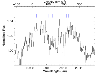
Figure 5.— The 2.91 $\mu$m H₂O emission lines. The blue tick marks indicate the positions of the dominant transitions contributing to the emission feature. The zero velocity bin is centered at 2.90813 $\mu$m, the transition with the shortest wavelength of the list in Table 2 found in this spectral region. The upper x-axis gives the velocity space information and shows a Doppler shift of 24.4 km s^-1. H₂O transition information can be found in Table 2.

3.3. CO Observations

In order to self-consistently determine the column densities of CO, OH, and H₂O, we also present $K-$band observations of HD 101412. We reproduce the results of Cowley et al. (2012) and Ilee et al. (2014) in that we detect both the CO $\nu$ = 2 $\rightarrow$ 0 and $\nu$ = 3 $\rightarrow$ 1 bandheads. We determine the signal-to-noise of the chips containing the CO $\nu$ = 2 $\rightarrow$ 0 bandhead and isolated emission features (Chips 2 and 3) to be $\sim$290, while Chip 4, containing the $\nu$ = 3 $\rightarrow$ 1 bandhead emission, has a signal-to-noise of $\sim$120. Figure 6 shows the isolated CO $\nu$ = 2 $\rightarrow$ 0 emission lines (Chip 3), while Figure 7 show the CO $\nu$ = 2 $\rightarrow$ 0 (left) and $\nu$ = 3 $\rightarrow$ 1 (right) bandhead emission. Discussion of the modeling is presented in Section 4.

4. Modeling

To determine the spatial location, column density, and temperature of the CO, OH, and H₂O emission, we fit the spectra using a slab model (Carr et al., 2004). The disk models assume LTE and Keplerian rotation. Because we find that the emission originates in a fairly narrow annulus, the gas temperature and the column density for each species are taken to be constant over the emitting region.

We start by fitting the velocity profile of the CO $\nu$ = 2 $\rightarrow$ 0 lines, because the CO spectrum covers the greatest range of energy levels and has the highest signal-to-noise. The CO lines near 2.31 $\mu$m (Figure 6) are separated from other lines and give a clean measure of the line profile. A composite profile is formed using the four lines least affected by telluric absorption. A Keplerian disk emission model is fit to the profile using $\chi^{2}$ minimization, which gives 50.5 km s^-1 for the projected velocity at the inner radius of the emitting region, and 42.1 km s^-1 at the outer radius (or equivalently, R_out/R_in = 1.44). A third fit parameter is the exponent of a power law for the radial intensity, I $\propto$ r^α; however, the result is insensitive to this parameter, due to the small radial extent of the emission, and the exponent is set to a fixed value of $\alpha$ = $-$2.

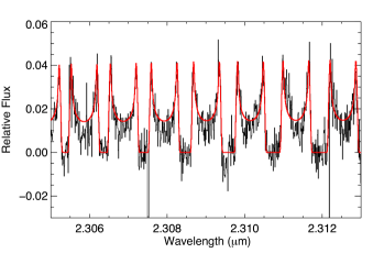
Figure 6.— Isolated CO $\nu$ = 2 $\rightarrow$ 0 emission lines. The best fit model is plotted in red. Final parameters for the model are T = 1300 K, N(CO) = 7 $\times$ 10²⁰ cm^-2, with R_in = 0.88 and R_out = 1.27 AU, and i = 86$\arcdeg$.

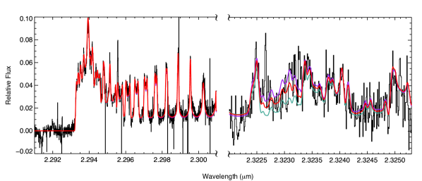
Figure 7.— CO $\nu$ = 2 $\rightarrow$ 0 (left) and 3 $\rightarrow$ 1 (right) bandhead emission modeling. The best fit model is plotted in red. Final parameters for the red model are the same as in Figure 6. Data is plotted in black, with the turquoise model indicating a temperature of 1000 K, red has a temperature of 1300 K, and purple has a temperature of 1500 K. The model is most sensitive to the region near 2.323$\mu$m.

Having set the kinematics of the CO emission, the CO $\nu$ = 2 $\rightarrow$ 0 bandhead and isolated lines are fit with a disk emission model. Given the narrow radial extent of the emission, the CO column density, N(CO), and temperature, T, are taken to be constant with radius. The main parameters that determine the bandhead shape and relative line intensities are T and N(CO). If you hold T constant, increasing N(CO) will increase the luminosity of the emission lines. For a given T and N(CO), matching the CO emission flux gives the projected emitting area, which is characterized by the radius of an equivalent circular area. The shape of the bandhead is also affected to a lesser degree by the local line broadening; the local line width was initially set to the CO thermal width. We find that the model fits to the CO $\nu$ = 2 $\rightarrow$ 0 bandhead have a large degeneracy between T and N(CO). Acceptable fit temperatures range from 1000 K to 2500 K, and we rule out emission for temperatures above 3000 K or below 800 K. When the CO $\nu$ = 3 $\rightarrow$ 1 bandhead is included in the fit, the relative flux of the $\nu$ = 3 $\rightarrow$ 1 and $\nu$ = 2 $\rightarrow$ 0 emission restricts the range in T and N(CO), removing the degeneracy from fitting the CO $\nu$ = 2 $\rightarrow$ 0 alone (Figure 7).

The best fit parameters for the CO overtone emission are T = 1300${}^{+200}_{-300}$ K and N(CO) = 7.0${}^{+6.9}_{-1.3}$ $\times$ 10²⁰ cm^-2, and the projected emitting area, $\pi$R${}_{\rm{e}}^{2}$, has a radius of R_e = 0.156 AU. This model is overplotted in red on the CO $\nu$ = 2 $\rightarrow$ 0 and $\nu$ = 3 $\rightarrow$ 1 bandheads in Figure 7, along with models for higher and lower temperatures.

Once we have the emitting column and projected area, we can break the degeneracy between disk inclination and radius by finding the inclination that is consistent with both the projected velocity and the projected emitting area. For the above solution, this inclination is i = 86$\arcdeg$. The inner and outer radii for the CO emission are then are R_in = 0.88, R_out = 1.27 AU

We also investigate the impact of non-thermal broadening (turbulence). The thermal width of CO at 1300 K is 1.5 km s^-1 (FWHM). Different amounts of extra broadening are added to the thermal width and the CO composite profile is refit. Then, the fits to the $\nu$ = 2 $\rightarrow$ 0 bandhead are repeated. A change in the local linewidth alters the overlap of the closely spaced transitions at the bandhead. Because the CO lines are optically thick, the amount of overlap affects the relative distribution of flux with wavelength and hence the shape of the bandhead. As the turbulence becomes larger, the fit to the shape at the bandhead becomes progressively worse. Based on this, we rule out v_turb (FWHM) $\geq$ 3.5 km s^-1 (Figure 8).

In modeling the OH, we first determine the radial extent of the OH emission by modeling the profile of the blended OH P4.5 doublet feature, using the same procedure used for the CO profile. Using the same inclination angle (86$\arcdeg$) from the CO modeling, the OH emitting region extends from R_in = 0.81 to R_out = 1.46 AU. Figure 2, panel A shows the model fit to the P4.5 doublet. The model includes non-thermal line broadening (FWHM) of 6.7 km s^-1, which improves the appearance of the fit at the peaks of the OH emission; however, the statistical significance, vs. thermal broadening, is small, and its inclusion does not change the derived radii for the emission. The same best fit velocity profile is consistent with the P5.5 emission feature, as show in Figure 2, panel C.

The OH and CO emission originate from similar radii, but the radial extent (and area) of the OH emission is somewhat larger than that found for the CO emission. Given that the CO and OH spectra were obtained 2 years apart, it is not clear whether the OH and CO line profiles point due to an intrinsic difference in their respective radial distributions or reflect the variability of the emitting size.

In order to derive a column density for the OH emission, we adopt the temperature of 1300 K found for CO, since the the OH features give no constraint on the gas temperature. Using the projected area for the OH emission, the column density is adjusted to match the flux in the OH P4.5 doublet. We find that N(OH) = 2.8${}^{+1.4}_{-0.7}$ $\times$ 10¹⁸ cm^-2, which yields a ratio of N(OH)/N(CO) = 4.0${}^{+2.3}_{-2.5}$ $\times$ 10^-3.

Modeling of the H₂O emission is more complicated. We originally confirmed our identification of these features as water by comparison to emission from LTE slab models. Due to the lower signal-to-noise of the H₂O emission, we find that it is not possible to uniquely determine the temperature and column density of water from the spectrum, although it is clearly hot, in the range of 1000 to 3000 K. In addition, the velocity line profile can not be constrained to the accuracy that is possible for CO and OH. Hence, the OH velocity profile and emitting area are used for H₂O, along with the same 1300 K temperature. The column density required to match the H₂O flux is N(H₂O) = 5.8${}^{+0.6}_{-0.8}$ $\times$ 10¹⁷ cm^-2. This model is compared to the H₂O emission features in Figure 9. Other features, outside of those mentioned in Section 3.2, are consistent with the H₂O emission model. The adopted parameters are consistent with the relative fluxes and velocity widths in the H₂O spectrum. The derived water column density yields ratios of N(H₂O)/N(OH) = 0.21${}^{+0.11}_{-0.06}$ and N(H₂O)/N(CO) = 8.3${}^{+3.0}_{-4.1}$ $\times$ 10^-4.

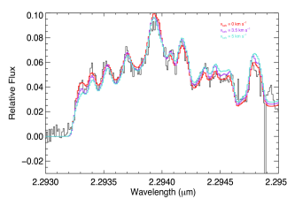
Figure 8.— Models of the CO $\nu$ = 2 $\rightarrow$ 0 bandhead for different levels of turbulent broadening compared to the observed spectrum. The nominal model, with only thermal broadening, is plotted in red. The turquoise model includes an additional broadening (FWHM) of 5.0 km s^-1, which corresponds to the total linewidth of 5.2 km s^-1 in Ilee et al. (2014). We rule out v_turb (FWHM) $>$ 3.5 km s^-1 (purple plot).

5. Comparison to other Young Stellar Objects

To contextualize our detection of water in the inner disk around HD 101412, we compare the column densities of CO, OH, and H₂O among seven other young stars for which water has been detected (HD 259431 does not have a detection of NIR water emission, just an upper limit on the water column density) (Table 3). SVS 13 is a $\geq 3$M_☉ (Hirota et al., 2008) young stellar object on the Class 0/Class I boundary (Chen et al., 2009) from which the CO $\nu$ = 2 $\rightarrow$ 0 bandhead and H₂O emission lines near 2.2935 $\mu$m have been observed (Carr et al., 2004). AS 205A, DR Tau, and RU Lup are all classical T Taruri stars (CTTS; spectral type K0, K5, and G5, respectively) around which CO, OH, and H₂O emission has been observed (Salyk et al., 2008; Mandell et al., 2012). V1331 Cyg is a 2.8 M_☉ intermediate mass T Tauri star (IMTTS; spectral type G7-K0; Petrov et al. 2014). Doppmann et al. (2011) observed OH and H₂O emission in the $L$-band from this star. 08576nr292 is a massive young stellar object (MYSO; $\sim$6 M_⊙ B5 star) from which H₂O and CO bandhead emission have also been detected (Thi & Bik, 2005).

For four of the sources (HD 101412, SVS 13, V1331 Cyg, and 08576nr292) in Table 3, CO column density is comparable (0.7-6 $\times$ 10²¹ molecules cm^-1). Three other source (AS 205A, DR Tau, and HD 259431) have much lower CO column density reported, ranging from 0.6-1.6 $\times$ 10¹⁹ molecules cm^-1 (RU Lup only has column density ratios reported in Mandell et al. 2012). However, even with the range in column densities, the ratios between molecules show similar trends when comparing similar sources. Lower mass T Tauri stars have N(OH)/N(CO) of a 2-3.3 $\times$ 10^-2 and N(H₂O)/N(CO) of 0.6-3.0 $\times$ 10^-1. As you move to more massive sources, this trend changes. N(OH)/N(CO) is now 0.5-4 $\times$ 10^-3 and N(H₂O)/N(CO) is 0.2-8 $\times$ 10^-4. The fact that the latest type star is surrounded by the disk with the highest H₂O/CO ratio suggests that the UV radiation from the star plays a pivotal role in determining the abundance of water in the atmosphere of the inner disk

In addition to the comparison among a handful of young stars for which water has been detected, we compare a sample of 19 T Tauri and HAeBe stars reported in the literature for which both OH and H₂O are measured (Table 4; Fedele et al. 2011; Banzatti et al. 2017). Plotting the OH line luminosity versus the H₂O line luminosity, we find that the T Tauri stars follow a linear trend given by Eqn. 1, confirming the constant OH/H₂O line flux ratios presented in Banzatti et al. (2017),

$$L_{H_{2}O}/L_{\sun}=(2.1\pm 0.1)L_{OH}/L_{\sun}+(0.09\pm 0.23).$$ (1)

Table 3Column Density Comparison to other YSOs

Star	SpT	M⋆	Class	N(CO)	N(OH)	N(H2O)	N(OH)/N(CO)	N(H2O)/N(CO)
		(M☉)		(cm-2)	(cm-2)	(cm-2)
SVS 131	–	3.0	Class 0/1	1.2 $\times$ 1021	–	1.8 $\times$ 1021	–	1.5
DR Tau2	K5	0.8	CTTS	7.0 $\times$ 1018	2.0 $\times$ 1017	8.0 $\times$ 1017	2.9 $\times$ 10-2	1.1 $\times$ 10-1
AS 205A2	K0	1.2	CTTS	6.0 $\times$ 1018	2.0 $\times$ 1017	6.0 $\times$ 1017	3.3 $\times$ 10-2	1.0 $\times$ 10-1
V1331 Cyg3	G7-K0	2.8	IMTTS	6.0 $\times$ 1021	1.0 $\times$ 1020	2.0 $\times$ 1021	2.0 $\times$ 10-2	3.0 $\times$ 10-1
RU Lup4	G5	0.7	CTTS	–	–	–	1.6 - 3.3 $\times$ 10-2	5.5 $\times$ 10-2
HD 101412	B9.5	2.5	HBe	7.0${}^{+6.9}_{-1.3}$ $\times$ 1020	2.8${}^{+1.4}_{-0.7}$ $\times$ 1018	5.8${}^{+0.6}_{-0.8}$ $\times$ 1017	4.0${}^{+2.3}_{-2.5}$ $\times$ 10-3	8.3${}^{+3.0}_{-4.1}$ $\times$ 10-4
08576nr2925	B5	6.0	MYSO	3.9 $\times$ 1021	–	2.5 $\times$ 1018	$\sim$1.0 $\times$ 10-3	6.4 $\times$ 10-4
HD 2594316,7	B5	6.6	HBe	1.6 $\times$ 1019	7.9 $\times$ 1015	$<$3.2 $\times$ 1014	4.9 $\times$ 10-4	$<$2.0 $\times$ 10-5

Note. — Comparison of molecular column densities from previously reported observations of young stellar objects. Thi & Bik (2005) did not observe OH emission in 08576nr292. N(OH)/N(CO) for 08576nr292 is based off chemical models. 1. Carr et al. (2004); 2. Salyk et al. (2008); 3. Doppmann et al. (2011); 4. Mandell et al. (2012); 5. Thi & Bik (2005); 6. Ilee et al. (2014); 7. Fedele et al. (2011);.

Among the sources included in this sample is EX Lupi while it was undergoing an outburst and in quiescence (Banzatti et al., 2017). The lumiosity increases along the fit to the T Tauri data indicating that the ratio of L${}_{\rm{H_{2}O}}$ and L_OH is relatively constant over a wide range of stellar luminosities. However, it is not clear if the FUV luminosity of the star would impact the emission from the circumstellar disk while undergoing an outburst. During outbursts, the inner disk heats up to the point that the continuum emission from the inner region buries the emission from the star. The outer disk would thus only see emission from the self-luminous inner disk. For example, the FUV spectra of T Tauri stars is more similar to FUors than to the far more FUV luminous HAeBes (Valenti et al., 2000).

While HD 101412 is the only HAeBe in the sample for which both water and OH are detected, upper limits for eight additional sources are available from Fedele et al. (2011). We find that the HAeBes consistently show weaker water luminosity for a given OH luminosity than the T Tauris. This trend is also suggestive that the UV luminosity of the stars plays an important role in determining the relative column density of water.

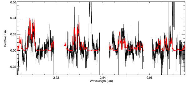
Figure 9.— Model of observed H₂O emission features. The model uses the same geometry as the best fit OH P4.5 model: R_in = 0.81 AU, R_out = 1.46 AU, and an inclination angle of 86$\arcdeg$.

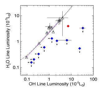
Figure 10.— Comparison of the H₂O line luminosity to the OH line luminosity taken from literature (Banzatti et al., 2017; Fedele et al., 2011) for T Tauri and HAeBe stars. T Tauri stars are plotted as open black triangles, HAeBe stars as blue diamonds, and HD 101412 as a red diamond. The black line is a weighted linear least squares fit to the T Tauri data. We do not plot T Tauri sources with upper limits from Banzatti et al. (2017), only T Tauris with detections of both water and OH at 2.9 $\mu$m. We only plot the HAe/Be sources with OH detections or upper limits and water upper limits for 2.9 $\mu$m from Fedele et al. (2011), and we have converted HAeBe upper limits to 1$\sigma$ levels for consistency. The purple line connects EX Lup observations from 2008 and 2014. The 2008 observation occurred during an accretion outburst resulting in higher OH and H₂O fluxes. The luminosity of the water emission from the T Tauri stars is consistently larger than the upper limits placed on HAeBe stars.

6. Discussion

Table 4H₂O Line Luminosity vs. OH Line Luminosity for YSOs

Star	SpT	M⋆	Class	L${}_{\rm{H_{2}O}}$	LOH
		(M☉)		(10-5 L☉)	(10-5 L☉)
AS 205A	K0	1.2	CTTS	3.76 $\pm$ 1.39	1.06 $\pm$ 0.39
DF Tau	K5	0.8	CTTS	2.19 $\pm$ 0.28	0.79 $\pm$ 0.10
DR Tau	M3	0.5	CTTS	3.41 $\pm$ 0.52	0.96 $\pm$ 0.14
EX Lup08	M0	0.8	CTTS	6.79 $\pm$ 2.04	3.03 $\pm$ 0.91
EX Lup14	–	–	–	0.25 $\pm$ 0.02	0.09 $\pm$ 0.01
RU Lup	K7-M0	0.7	CTTS	3.42 $\pm$ 0.48	1.28 $\pm$ 0.18
S Cra N	G0	0.6	CTTS	6.36 $\pm$ 1.97	2.75 $\pm$ 0.85
T Tau N	K1.5	2.4	IMTTS	8.28 $\pm$ 6.63	3.98 $\pm$ 3.18
VW Cha	K7	0.6	CTTS	2.39 $\pm$ 0.13	1.52 $\pm$ 0.08
VZ Cha	K7	0.8	CTTS	0.85 $\pm$ 0.01	0.35 $\pm$ 0.01
BF Ori	A5	1.4	HAe	$<$0.16	$<$0.16
HD 34282	A0	1.9	HAe	$<$0.20	$<$0.20
HD 76534	B2	11.4	HBe	$<$1.51	$<$1.51
HD 85567	B5	6	HBe	$<$3.32	33.19 $\pm$ 9.96
HD 98922	B9	5.2	HBe	$<$0.40	$<$0.40
HD 101412	B9.5	2.5	HBe	3.96 $\pm$ 0.30	7.18 $\pm$ 0.25
HD 250550	B7	3.6	HBe	$<$1.06	2.23 $\pm$ 0.16
HD 259431	B5	6.6	HBe	$<$0.55	23.86 $\pm$ 3.29
UX Ori	A3	2.1	HAe	$<$0.33	$<$0.33
V380 Ori	A1	2.8	HAe	$<$1.13	6.31 $\pm$ 3.75

Note. — Luminosity values from literature used in Figure 10. T Tauri flux values are obtained from Banzatti et al. (2017), and HAeBe flux values and upper limits from Fedele et al. (2011). Flux values are converted to luminosities using distances obtained from Gaia Collaboration et al. (2016). Upper limits have been converted to 1$\sigma$ limits for consistency.

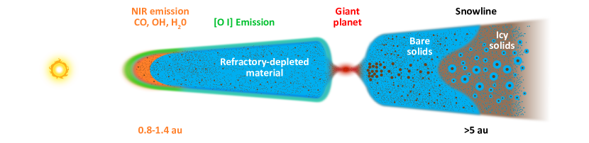
Figure 11.— The above schematic presents one possible scenario, discussed in detail in the text, to explain the NIR observations of HD 101412. Based on the stellar luminosity for HD 101412, we determine the dust sublimation radius to be at 0.25 AU. The molecular emission arises from a narrow annulus ($\sim$0.8 - 1.4 AU). Refractory elements are observed to be below solar abundances based on photospheric observations, while C and O are found to be at solar abundances (Folsom et al., 2012). This indicates that large dust grains are filtered out, leading to a depletion of refractory elements in the inner disk. If a planetary body was forming within the snow line ($>$5 AU), this would allow for C- and O-containing molecules to reside in the inner disk, eventually accreting onto the central star and giving rise to the observed photospheric abundance pattern. This figure is not to scale.

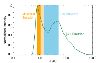
Figure 12.— Updated Figure 8 from Fedele et al. (2008) showing locations of [O I] emission, dust emission, and molecular emission from HD 101412. The orange indicates the location of OH, H₂O, and CO gas presented from our analysis. The blue region indicates the dust emission based on MIDI observations, updated to account for the Gaia Collaboration et al. (2016) distance. The light brown is the overlap of the two regions, with the [O I] emission (in green) remaining unchanged due to the use of similar stellar masses between the studies.

The infrared molecular emission from HD 101412 is unusual in several respects. Firstly, we see the CO bandhead emission arising from a narrow annulus. To populate the CO bandheads, the gas must be hot (T $\gtrsim$ 2000 K) and dense (n${}_{H}\gtrsim 10^{10}$ cm²; Najita et al. 1996). The requisite conditions are ordinarily only met in systems with high accretion rates ($\sim$10${}^{-7}-10^{-6}$ M_⊙yr^-1, Ilee et al. 2014). CO bandhead emission is rarely observed in HAeBe systems, with a detection rate of 7% (Ilee et al., 2014).

In order to detect the large columns of CO gas observed in emission, all CO bandhead sources require strong suppression of the $K-$band opacity in the CO-emitting region. For HD 101412, the CO column density inferred from overtone bandhead emission (7$\times$10²⁰ cm^-2; Table 3) corresponds to N_H=1.4$\times$10²⁵ cm^-2, assuming a CO/H₂ of 1 $\times$ 10^-4 or an A_K = 600 if the dust were interstellar. Detecting a CO column as large as $7\times 10^{20}$ cm^-2 therefore requires a reduction in the K-band continuum opacity by a factor of $\sim$600, i.e., a factor of $\sim$6 larger than the typical factor of $\sim$100 reduction in grain surface area that is found for T Tauri disks (Furlan et al., 2007).

Ilee et al. (2014) mention that CO emission is primarily observed around B-type stars, which makes sense due to the required temperatures to excite CO bandhead emission. Conditions around lower mass stars may only reach requisite temperatures during episodic accretion events thus resulting in variable CO bandhead emission. Also, due to the high gas density required, some disks may lack sufficient material to allow for CO bandhead emission. Ilee et al. (2014) also mention a possible connection to high disk inclinations with CO bandhead emission. Their sources with detections had a range of inclinations from 51$\arcdeg$ to 72$\arcdeg$, based on model fits. A possible explanation for this inclination dependance would be the CO bandhead emission tracing the inner disk wall near the dust sublimation radius.

Secondly, whereas water emission is rare among HAeBe disks (Section 1), we detect in HD 101412 hot water emission with a luminosity comparable to the most luminous water emission from T Tauri disks. One possible explanation for the dearth of water emission from HAeBe disks compared to T Tauri disks is the relative UV luminosities to which the circumstellar disks are exposed: the strong FUV field of HAeBe stars can readily dissociate water in their disk atmospheres. This may not be apparent from the Walsh et al. (2015) chemical model of a disk around a HAe star, which finds a water-rich disk atmosphere with water column densities much larger than is consistent with observations. As they note, one reason for the discrepancy between the observed and predicted water columns may be their assumption of interstellar grains (gas-to-dust ratio and grain size distribution), which limits the penetration depth of the UV photons and their effect on disk molecular abundances.

The T Tauri disk models of Ádámkovics et al. (2014) (their Figure 4; see also Ádámkovics et al. (2016) and Najita & Ádámkovics (2017)) support this perspective. Assuming grain growth at the level inferred for observed sources (e.g., Furlan et al. 2007), these models find that increasing the FUV radiation from T Tauri stars does in fact push the molecular layer deeper into the disk and dissociates H₂O to produce more extensive OH. Models of HAeBe disks that assume a comparable level of grain growth, would likely find a similar reduction in the water column density in the disk atmosphere, more consistent with the general lack of water emission detected from HAeBe stars (Figure 10). In principle, water emission could be detected in HAeBe disks if the dust opacity in the disk atmosphere was low enough that the dust photosphere was located below the transition from OH to H₂O.

There are reasons to expect a low dust opacity in the inner disk of HD 101412. The stellar photosphere of HD 101412 is strongly depleted in refractory elements (Fe, Mg, Si), but has solar-like abundances of volatile elements (C, N, O), thus, HD 101412 is a $\lambda$ Boö star (Folsom et al., 2012). Kama et al. (2015) hypothesize that the depletion of heavy elements in the photosphere of the star is a consequence of selective accretion of gas relative to dust, that is the accreting material accreting has a gas-to-dust ratio of $\sim$600, i.e., a reduction in refractories by a factor of $\sim 6$, similar to the extra factor of 6 reduction needed in the K-band continuum opacity to expose the entire CO bandhead-emitting column to view.

What is the source of the depletion of refractory material in the disk? If a giant planet (with mass from 0.1 M_J to 10 M_J) is present in the disk, the pressure bumps it creates (e.g., at the edge of a gap) could preferentially reduce the accretion of solids relative to gas through the disk by aerodynamic drag (Rice et al., 2006; Zhu et al., 2012). Due to the lack of a convective outer layer in early-type stars, the refractory depleted material that accretes onto the star would reside on the surface, giving rise to the $\lambda$ Boö abundance pattern (Figure 11).

The detection of C- and O-bearing molecules (CO, OH, and H₂O) from the inner region of the HD101412 disk and the detection of CO₂ with Spitzer (Pontoppidan et al., 2010), which presumably will eventually accrete onto the star, is consistent with the high abundance of volatile elements in the stellar atmosphere of HD 101412. The presence of oxygen-bearing molecules such as H₂O and CO₂ in the gas phase implies that if a planet induced gap is responsible for filtering out the solids from the inwardly accreting material (Kama et al., 2015), the planet would likely be located well inward of the snow line (which we estimate is located at $\sim$25 AU adopting the distance at which a blackbody is 150K, but must lie beyond 5 au; Figure 11). If the planet were located near or beyond the snow line, dust filtering would remove water ice (and oxygen) as well from the accreting material, creating a more carbon-rich composition, in which molecules like H₂O and CO₂ are unlikely to be abundant (Figure 11).

The NIR molecular emission from HD 101412 overlaps the [O I] emission from the source and is roughly coincident spatially with the inner edge of the dust disk seen in the mid-infrared. The mid-infrared dust emission arises from 1.1 - 5.2 AU when taking into consideration the new distance from Gaia (Figure 12; Fedele et al. 2008; van der Plas et al. 2008).The structure shown in Figure 12 is analogous to a miniature photo dissociation region with the inner emission arising from [O I], then molecular emission, followed by dust emission. The [O I] emission probes the tenuous atomic layer of the disk that is depleted of dust and molecules. It is not clear what the radial extent of the disk is as there are presently no far-infrared or submillimeter observations that would probe the cooler dust arising from beyond 5 AU.

Given the high inclination of the system (i = 86$\arcdeg$; Section 4), the hot molecular emission we see may be coming from the inner wall of the far side of the disk. A viewing angle 4$\arcdeg$ from edge-on appears large enough to obtain an unobstructed view of the bright molecular emission from the far side of the inner disk. Given the temperature of the molecular emission (1300 K; Section 4) and the stellar mass (2.5 M_⊙; Section 1), the disk scale height at the radius of the molecular emission (1 AU) is 0.05 AU if the gas is in hydrostatic equilibrium; thus the height of the molecular emitting gas on the near side of the disk may rise $\sim$1.5$\arcdeg$ above the midplane when viewed from the far side of the disk 2 AU away.

There are two observational approaches to test our hypothesis that the luminosity of the water emission and CO bandhead emission are enhanced by the depletion of dust in the inner disk (by a factor of 6 or more; Kama et al. 2015). Firstly, one can compare the equivalent width of the molecular emission to the gas-to-dust ratio of the accreting material as inferred from photospheric abundances of the star. Larger molecular emission equivalent widths are expected for systems with larger gas-to-dust ratios. Secondly, one can test the role of the disk inclination by observing additional edge-on systems and comparing these to more inclined systems. The emission from the edge-on systems will be dominated by the inner wall of the disk and should probe denser gas than the more face-on systems where the emission is dominated by less dense gas from the disk surface.

The feasibility of this scenario can also be tested through thermochemical modeling of the inner disk. One possible concern is that if grains are too under-abundant, it is difficult to synthesize H₂ on grains, a critical first step in the gas phase synthesis of molecules such as OH, CO and water. Severe dust depletion may make it difficult to counteract photodestruction of molecules and sustain a substantial reservoir of molecular gas. Self-consistently fitting the infrared portion of the SED and molecular column density in the disk atmosphere will inform the feasibility of our hypothesis.

7. Conclusions

We present the first detection of water emission at 2.9 $\mu$m in a Herbig Ae/Be star system, along with a new detection of OH ro-vibrational emission. The OH emission observed represents the strongest ever observed in a HAeBe disk in terms of line-to-continuum ratio. The observed line profiles for both OH and H₂O indicate that the emitting region for both molecules is narrow and $\sim$1 AU from the star.

The bright molecular emission from HD 101412 may be related to its photospheric abundance pattern, i.e., its nature as a $\lambda$ Boö star, and the disk’s large inclination angle. If the low abundance of refractory elements is a result of selective accretion of gas relative to dust, as has been previously hypothesized, the inner disk from which HD 101412 accretes should be strongly dust-depleted and its continuum more optically thin. This situation would tend to produce strong molecular emission from the inner disk, as is observed. Our detection of C- and O-bearing molecules from the inner disk is consistent with the expected presence in this scenario of abundant volatiles in the accreting material.

References

- Ádámkovics et al. (2014) Ádámkovics, M., Glassgold, A. E., & Najita, J. R. 2014, ApJ, 786, 135
- Ádámkovics et al. (2016) Ádámkovics, M., Najita, J. R., & Glassgold, A. E. 2016, ApJ, 817, 82
- Banzatti & Pontoppidan (2015) Banzatti, A., & Pontoppidan, K. M. 2015, ApJ, 809, 167
- Banzatti et al. (2017) Banzatti, A., Pontoppidan, K. M., Salyk, C., et al. 2017, ApJ, 834, 152
- Blake & Boogert (2004) Blake, G. A., & Boogert, A. C. A. 2004, ApJ, 606, L73
- Brittain et al. (2016) Brittain, S. D., Najita, J. R., Carr, J. S., Ádámkovics, M., & Reynolds, N. 2016, ApJ, 830, 112
- Brittain et al. (2007) Brittain, S. D., Simon, T., Najita, J. R., & Rettig, T. W. 2007, ApJ, 659, 685
- Brown et al. (2013) Brown, J. M., Pontoppidan, K. M., van Dishoeck, E. F., et al. 2013, ApJ, 770, 94
- Carr et al. (2004) Carr, J. S., Tokunaga, A. T., & Najita, J. 2004, ApJ, 603, 213
- Chen et al. (2009) Chen, X., Launhardt, R., & Henning, T. 2009, ApJ, 691, 1729
- Cowley et al. (2012) Cowley, C. R., Hubrig, S., Castelli, F., & Wolff, B. 2012, A&A, 537, L6
- Doppmann et al. (2011) Doppmann, G. W., Najita, J. R., Carr, J. S., & Graham, J. R. 2011, ApJ, 738, 112
- Fairlamb et al. (2015) Fairlamb, J. R., Oudmaijer, R. D., Mendigutía, I., Ilee, J. D., & van den Ancker, M. E. 2015, MNRAS, 453, 976
- Fairlamb et al. (2017) Fairlamb, J. R., Oudmaijer, R. D., Mendigutia, I., Ilee, J. D., & van den Ancker, M. E. 2017, MNRAS, 464, 4721
- Fedele et al. (2012) Fedele, D., Bruderer, S., van Dishoeck, E. F., et al. 2012, A&A, 544, L9
- Fedele et al. (2011) Fedele, D., Pascucci, I., Brittain, S., et al. 2011, ApJ, 732, 106
- Fedele et al. (2008) Fedele, D., van den Ancker, M. E., Acke, B., et al. 2008, A&A, 491, 809
- Fedele et al. (2013) Fedele, D., Bruderer, S., van Dishoeck, E. F., et al. 2013, A&A, 559, A77
- Folsom et al. (2012) Folsom, C. P., Bagnulo, S., Wade, G. A., et al. 2012, MNRAS, 422, 2072
- Furlan et al. (2007) Furlan, E., Sargent, B., Calvet, N., et al. 2007, ApJ, 664, 1176
- Gaia Collaboration et al. (2016) Gaia Collaboration, Brown, A. G. A., Vallenari, A., et al. 2016, A&A, 595, A2
- Gaia Collaboration et al. (2018) —. 2018, A&A, 616, A1
- Hirota et al. (2008) Hirota, T., Bushimata, T., Choi, Y. K., et al. 2008, PASJ, 60, 37
- Hubrig et al. (2010) Hubrig, S., Schöller, M., Savanov, I., et al. 2010, Astronomische Nachrichten, 331, 361
- Ilee et al. (2014) Ilee, J. D., Fairlamb, J., Oudmaijer, R. D., et al. 2014, MNRAS, 445, 3723
- Kama et al. (2015) Kama, M., Folsom, C. P., & Pinilla, P. 2015, A&A, 582, L10
- Käufl et al. (2004) Käufl, H.-U., Ballester, P., Biereichel, P., et al. 2004, in Proc. SPIE, Vol. 5492, Ground-based Instrumentation for Astronomy, ed. A. F. M. Moorwood & M. Iye, 1218–1227
- Kunde & Maguire (1974) Kunde, V. R., & Maguire, W. C. 1974, J. Quant. Spec. Radiat. Transf., 14, 803
- Mandell et al. (2012) Mandell, A. M., Bast, J., van Dishoeck, E. F., et al. 2012, ApJ, 747, 92
- Mandell et al. (2008) Mandell, A. M., Mumma, M. J., Blake, G. A., et al. 2008, ApJ, 681, L25
- Meeus et al. (2012) Meeus, G., Montesinos, B., Mendigutía, I., et al. 2012, A&A, 544, A78
- Najita et al. (1996) Najita, J., Carr, J. S., Glassgold, A. E., Shu, F. H., & Tokunaga, A. T. 1996, ApJ, 462, 919
- Najita & Ádámkovics (2017) Najita, J. R., & Ádámkovics, M. 2017, ApJ, 847, 6
- Ochsenbein et al. (2000) Ochsenbein, F., Bauer, P., & Marcout, J. 2000, A&AS, 143, 23
- Petrov et al. (2014) Petrov, P. P., Kurosawa, R., Romanova, M. M., et al. 2014, MNRAS, 442, 3643
- Pontoppidan et al. (2010) Pontoppidan, K. M., Salyk, C., Blake, G. A., et al. 2010, ApJ, 720, 887
- Rice et al. (2006) Rice, W. K. M., Armitage, P. J., Wood, K., & Lodato, G. 2006, MNRAS, 373, 1619
- Rothman et al. (2003) Rothman, L. S., Barbe, A., Benner, D. C., et al. 2003, J. Quant. Spec. Radiat. Transf., 82, 5
- Rothman et al. (2013) Rothman, L. S., Gordon, I. E., Babikov, Y., et al. 2013, J. Quant. Spec. Radiat. Transf., 130, 4
- Salyk et al. (2011a) Salyk, C., Blake, G. A., Boogert, A. C. A., & Brown, J. M. 2011a, ApJ, 743, 112
- Salyk et al. (2008) Salyk, C., Pontoppidan, K. M., Blake, G. A., et al. 2008, ApJ, 676, L49
- Salyk et al. (2011b) Salyk, C., Pontoppidan, K. M., Blake, G. A., Najita, J. R., & Carr, J. S. 2011b, ApJ, 731, 130
- Siess et al. (2000) Siess, L., Dufour, E., & Forestini, M. 2000, A&A, 358, 593
- Thi & Bik (2005) Thi, W.-F., & Bik, A. 2005, A&A, 438, 557
- Troutman (2010) Troutman, M. R. 2010, PhD thesis, Clemson University
- Valenti et al. (2003) Valenti, J. A., Fallon, A. A., & Johns-Krull, C. M. 2003, ApJS, 147, 305
- Valenti et al. (2000) Valenti, J. A., Johns-Krull, C. M., & Linsky, J. L. 2000, ApJS, 129, 399
- van der Plas et al. (2008) van der Plas, G., van den Ancker, M. E., Fedele, D., et al. 2008, A&A, 485, 487
- van der Plas et al. (2015) van der Plas, G., van den Ancker, M. E., Waters, L. B. F. M., & Dominik, C. 2015, A&A, 574, A75
- Walsh et al. (2015) Walsh, C., Nomura, H., & van Dishoeck, E. 2015, A&A, 582, A88
- Zhu et al. (2012) Zhu, Z., Nelson, R. P., Dong, R., Espaillat, C., & Hartmann, L. 2012, ApJ, 755, 6