Leader formation with mean-field birth and death models
Abstract.
We provide a mean-field description for a leader-follower dynamics with mass transfer among the two populations. This model allows the transition from followers to leaders and vice versa, with scalar-valued transition rates depending nonlinearly on the global state of the system at each time.
We first prove the existence and uniqueness of solutions for the leader-follower dynamics, under suitable assumptions. We then establish, for an appropriate choice of the initial datum, the equivalence of the system with a PDE-ODE system, that consists of a continuity equation over the state space and an ODE for the transition from leader to follower or vice versa. We further introduce a stochastic process approximating the PDE, together with a jump process that models the switch between the two populations. Using a propagation of chaos argument, we show that the particle system generated by these two processes converges in probability to a solution of the PDE-ODE system. Finally, several numerical simulations of social interactions dynamics modeled by our system are discussed.
1. Introduction
The mathematical modeling of collective behavior for systems of interacting agents has spawned an enormous wealth of literature in recent years. From the study of biological, social and economical phenomena [9, 2, 22, 1] to automatic learning [14, 35] and optimization heuristics [25, 36], these models lay at the heart of some of today’s most prominent lines of research: for the latest development in the field, we point to the surveys [8, 13, 18, 48] and references therein.
The modeling of such phenomena typically starts from particle-like systems as in statistical physics. These particle models are also called Agent Based Models, and they usually consist of a set of ODEs (one for each agent) interwined in a nonlinear way. Such a modeling approach is quite useful, with one of the main advantages being the explicit description of the mutual interaction among agents, but has huge problems to treat large systems of particles, as is the case with cells, molecules and social networks’ users. A classical approach to attack the problem is to pass to a continuous description of the system, which means to pass from a particle description to a kinetic descriptions where the unknown is the particle density distribution in the state space.
A useful tool in solving this problem is the mean-field limit [33], which amounts to replace the influence of all the other individuals in the dynamics of any given agent by a single averaged effect, a technique that goes back to [24] in plasma physics: to exemplify it, if applied to a Hegselmann-Krause-type discrete particle system over (see [34])
where denotes the interaction kernel (which models the interaction between particles) it leads to a continuity equation of Vlasov type
with denoting the probability distribution of the particles over the state space and
Notice how, in the process, the information of the pointwise positions is replaced by the knowledge of the space distribution of the particles . Such approach has the advantage of reducing the computational complexity of the models (overcoming the curse of dimensionality [10]) and allows the so-called microfundation of macromodels, i.e., the validation of the macroscopic dynamics from the coherence with the behavior of individuals (a central issue in the field of macroeconomics). The mean-field limit of systems of interacting agents has been thoroughly studied also in conjunction with irregular interaction kernel [17, 32], control problems [38, 30, 15, 29, 3] and multiple populations [21, 12, 4, 5]. Also models where the total mass of the system is not preserved in time, due to the presence of source (or sink) terms, have been considered (see for instance [45, Sections 4-5]). In other models, the total mass of the system is preserved, but not the role of the agents, since exchanges of mass between different populations are allowed. One of these models is the leader-follower dynamics studied in [27, 19], given by
| (1) |
Here, two competing populations and , of followers and leaders respectively, are in interaction. Both the masses of followers and leaders vary in time, while their sum is constant. The functionals for are interaction kernels, modeling their mutual spatial influence, while the transition rates govern the exchange of mass between and . In this paper, we shall provide a thorough mean-field analysis of (1), discussing its well-posedness and rigorously deriving it from an Agent Based Model. In order to do this, we will restrict our attention to the case where the transition rates are scalar-valued, that is they depend on the global state of the system at each time , but not explicitly on the position . The usefulness of such a simplification in our analysis is discussed later on in Remark 2.7.
In order to carry out our analysis, we shall first establish the well-posedness of (1) by means of a compactness argument in the space of finite positive measures with compact support endowed with the generalized Wasserstein distance , see [43]. To do so, we shall introduce an explicit Euler approximation of the dynamics and show that it converges, as the time step vanishes, to the unique solution of system (1).
We shall then prove the equivalence between (1) and another system for which we can more easily provide a particle dynamics. Intuitively, this equivalent system is introduced by defining the measures as111With a slight abuse of notation, from now on we write instead of .
The idea of the equivalence is that, under suitable hypotheses on the initial data, one can recover from by the relations
| (2) |
We shall show that, if the initial datum , satisfies (2) for , the system (1) is equivalent to
| (3) |
where is the product measure, the vector field for is
| (4) |
and the birth-death transition matrix is
| (5) |
The advantage of the measures and , with respect to and , is that they are probability measuers over and , respectively, and we can therefore use a propagation of chaos argument (see [46]) to show that there exists a sequence of stochastic processes whose mean-field limit for is system (3). We will actually provide such processes in explicit form: we denote them as , where for every and we have . Setting
then their dynamics is given by
-
•
-
•
obeys a jump process, with conditional transition rates for the realization of at time , given by
-
–
if then with rate ,
-
–
if then with rate .
-
–
By virtue of the equivalence between (1) and (3), the mean-field limit for of the above Agent Based Model is system (1).
The final part of our paper is devoted to numerical implementations of (1). Three model applications are considered:
-
•
consensus dynamics for two populations with a bounded confidence interaction kernel of Hegselmann-Krause type;
-
•
aggregation dynamics with competition among repulsive followers , and attractive leaders ;
-
•
the problem of steering a population towards a desired position via leaders’ action.
In the case of consensus we compare the effect of suitably chosen density-dependent birth and death rates, allowing the system to reach consensus, with constant ones, where instead the system ends up clustering around different states.
For the second case, observe that aggregation models are used to describe several biological phenomena, but also as building brick of social interactions such as crowd motion [23, 11]. We show that a controlled generation of leaders, with attraction kernel, is able to confine the whole density, balancing the repulsiveness of followers’ interactions.
In the third case, we study the case where leaders’ generation is conditioned to achievement of a desired position, in analogy with control problem for pedestrian dynamics [2, 16]. Thus leaders’ motion influences the followers’ density towards a specific goal, whereas followers’ interactions are ruled by an aggregation equation. We show that the whole population is steered to the desired state, with the leaders’ mass diminishing, and eventually vanishing, as soon as the followers are sufficiently close to the final state.
As a final remark we observe that most of our results can be straightforwardly extended to the case of a finite hierarchy of labels instead of with transitions given by
All the proofs would follow along the same lines, though at the expense of notation. Actually, we conjecture that the results of the paper hold true even in the case of a countable number of labels , as treated in a simplified scenario in [47].
A further issue, which falls for the moment outside the scope of our methods, and is likely to require a finer analysis, is the mean-field derivation of system (1) in the case where the birth rates take values in a functional space, for example when they explicitly depend on the position . We plan to address these aspects in future contributions.
The structure of the paper is the following. After discussing some measure-theoretical preliminaries in Section 2, we turn our attention to system (1). We introduce a general set of assumptions and prove the existence and uniqueness of solutions, using explicit Euler approximations of the dynamics and a compactness argument in the space of positive measures with bounded mass and compact support, endowed with the generalized Wasserstein distance . This is done in Section 3, where we also establish a bijection between solutions of (1) and of (3) under certain assumptions on the initial data (Proposition 3.4). In Section 4 we derive system (3) as mean-field limit of a particle system which couples a SDE (66) for the particles’ motion with a nonlinear master equation (67) for their labels. Section 5 is devoted to numerical experiments, which make use of the finite volume scheme discussed in B. In A we introduce some explicit examples of transition functionals which comply with our assumptions and are indeed used in the experiments of Section 5.
2. Preliminaries
Let be a Radon space; we denote by the set of finite positive measures on , and by the subset of finite positive measures with compact support. The space is the subset of whose elements are the probability measures on , i.e., those for which . The space is the subset of whose elements have finite -th moment, i.e.,
We denote by the subset of which consists of all probability measures with compact support. We denote the mass of a measure as .
If and are Radon spaces, for any222more in general, also if is a signed Borel measure on and any Borel function , we denote by the push-forward of through , defined by
In particular, if one considers the projection operators and defined on the product space , for every we call first (resp., second) marginal of the probability measure (resp., ). Given and , we denote by the subset of all probability measures in with first marginal and second marginal .
We denote the weak convergence of measures as follows:
2.1. The Wasserstein distance
In this section, we recall the definition of Wasserstein distance, as well as some of its useful properties.
Definition 2.1 (Wasserstein distance).
For every we define
| (6) |
Remark 2.2.
Remark 2.3.
We finally recall the following result, see e.g. [49].
Proposition 2.4.
Wasserstein distances are ordered, in the sense that implies
2.2. Solutions of transport equations
We now recall the precise definition of solutions to systems (1) and (3). Indeed, a solution of system (1) must be interpreted in the sense of distributions, as follows.
Definition 2.5 (Solution of system (1)).
Let be given, as well as . We say that the couple is a solution of system (1) with initial datum when
-
(1)
and ;
-
(2)
for each , the function is continuous with respect to the topology of weak convergence of measures;
-
(3)
there exists such that for every ;
-
(4)
for every and it holds
for almost every , with
Similarly, we introduce the concept of solution of system (3).
Definition 2.6 (Solution of system (3)).
Let be given, as well as and . We say that is a solution of system (3) with initial datum when
-
(1)
and ;
-
(2)
the function is continuous with respect to the topology of weak convergence of measures, while is absolutely continuous333It is sufficient to prove absolute continuity of one component only, since . ;
-
(3)
there exists such that ;
- (4)
Remark 2.7.
Throughout the paper it is assumed that the transition rates encoded by the matrix only depend on the global state of the system and not on the position . While being already useful at the level of deducing existence of solutions of (1), this restriction will be needed in order to show equivalence between solutions of (1) and (3), provided the initial datum is suitably chosen, satisfying Assumption (H1) below. This will be apparent in the proof of Proposition 3.4. As already discussed in the Introduction, this equivalence is a crucial step for the mean field derivation in Section 4.
2.3. The method of characteristics
In this section, we recall the method of characteristics to find solutions of transport equations. In particular, we recall the connection between the solutions of an ordinary differential equation with vector field and the solution to transport equations as the evolution of the corresponding probability distribution.
We start with the classical definitions of Carathéodory functions and solutions.
Definition 2.8.
A function is a Carathéodory function if
-
(1)
For all , the application is Lipschitz.
-
(2)
For all , the application is measurable.
-
(3)
There exists such that for all .
If the Lipschitz constant of the function belongs to , existence and uniqueness of Carathéodory solutions to (8) can be shown, see e.g. [28]. From now on, we denote by the flow of (8), i.e. the map that associates to each initial data the corresponding solution of (8) at time . Carathéodory solutions of finite dimensional systems and weak solutions of continuity equations are intimately related, as the following classical result shows.
Lemma 2.9.
Let be a Carathéodory function and be a Carathéodory solution of
Then is the unique weak solution of
| (9) |
As a consequence, if , then for each it holds
| (10) |
Moreover, consider the inhomogeneous transport equation
| (11) |
for being a measurable family (with respect to the weak topology of meaures) of signed Borel measures such that there exist with
for all .
Then, there exists a unique solution to (11), that satisfies the Duhamel’s formula
| (12) |
Here, is the flow of the non-autonomous vector field starting at time , i.e. the function that associates to the solution at time of
As a consequence, if , then for each it holds
| (13) |
Proof.
For the existence of a solution to (9), which is the push-forward of the initial datum via the flow map, see e.g. [49]. Uniqueness comes from standard arguments for the linear continuity equation, see e.g. [7].
We now prove (10). For a given , consider a test function with compact support, such that on . It then holds
| (14) |
Recall the elementary estimate for ordinary differential equations
Since for each it holds , then . Thus, the integral in (14) is zero. Since this holds for any test function with support outside , this implies that is supported in .
The proof of existence for the inhomogeneous case is similar. Duhamel’s formula is a re-writing of the method of variations of constants, that can be verified with direct computations. Uniqueness can be proved with the standard method: the difference between two solutions solves (9) with , then its unique solution is . The proof for (13) follows the proof for (10). ∎
2.4. The Generalized Wasserstein distance
The main technical issue about the transport equation (1) is that it mixes two different phenomena: on one side the non-local dynamics given by convolutions ; on the other side, sources and sink that make the total mass of non-constant.
It has been shown in several examples that the Wasserstein distance is a powerful tool to deal with transport equation with non-local vector fields, see e.g. [6, 42, 24, 33, 49]. Neverthelss, the Wasserstein distance is defined between measures with the same mass, hence it is not useful for problems in which the mass varies in time. This issue recently led to the development of a series of different generalizations of the Wasserstein distance to measures with different masses. See e.g. [20, 37, 39, 43].
In this article, we choose to use the generalized Wasserstein distance, that has been introduced in [43, 44]. Indeed, it has been already proved in [43] that, under suitable hypotheses written in terms of the generalized Wasserstein distance, transport equations with both non-local velocities and source terms admit existence and uniqueness of the solution.
We now recall the definition of the generalized Wasserstein distance, together with some key properties.
Definition 2.10.
Let be two measures. Given and , we define the functional
| (15) |
Proposition 2.11.
The following properties hold:
-
(1)
The functional is a distance on .
-
(2)
The distance metrizes the weak convergence on compact sets, i.e. given with it holds
-
(3)
The space is complete with respect to .
-
(4)
Let be two Lipschitz vector fields, with a Lipschitz constant for both . It then holds:
(16) (17) -
(5)
It holds
(18)
We now recall a result equivalent to the Kantorovich-Rubinstein duality for the generalized Wasserstein distance . It states that it coincides with the so-called flat distance, see e.g. [26].
Theorem 2.12.
Let . Then
As simple consequences, for it holds
| (19) | |||
| (20) |
The proof is given in [44].
From now on, we will only deal with the generalized Wasserstein distance , i.e. with the flat distance. For this reason, we will drop the parameters, and use the notation
Moreover, we use the same notation for the corresponding distance on : given and , we write
| (21) |
Finally, we use again the same notation for the supremum distance on : given and , we write
| (22) |
3. Well-posedness and equivalence for the leader-follower dynamics
We now turn our attention to system (1) and use the tools introduced in Section 2 to prove the existence and uniqueness of solutions. To do so, we will define a sequence of measures as explicit Euler approximations of the dynamics (1) and, by a a compactness argument in the space embedded with the generalized Wasserstein distance , we show that it converges, up to subsequences, to the unique solution of system (1). Next, we shall establish a bijection between solutions of (1) and of (3) under certain assumptions on the initial data. As a byproduct of the previous results, such equivalence yields the well-posedness of (3) as well, paving the way for the mean-field analysis of the subsequent sections.
3.1. Main assumptions
In this section we discuss the set of assumptions we shall assume henceforth. These assumptions assure, in particular, the existence and uniqueness of solutions of (1), as well as the equivalence between (1) and (3), that is more amenable to a mean-field analysis, as we will show in Section 4. We warn in advance the reader that Assumption (H1) below, differently from the other ones, is not needed for the existence result in Proposition 3.2, but will be used for the equivalence result in Proposition 3.4.
-
(H1)
There exist and such that and .
-
(H2)
there exists a constant such that, for every and , it holds
-
(H3)
there exists a constant such that, for every and , it holds
-
(H4)
there exists a constant such that for every and it holds
-
(H5)
there exists a constant such that, for every and satisfying
(23) and
(24) it holds
(25)
We now list some useful consequences of the previous hypotheses.
Proposition 3.1.
For and , we will use (as already done in (5)) the notations and to indicate the transition rates defined by
| (27) |
If (25) holds, it easily follows from the definition (15) that, for , satisfying (24) and , , we have
for . We additionally exploited above the inequality which immediately stems out of (15) whenever and are probability measures. If we endow the set with the usual distance on finite sets defined by
| (28) |
we can rewrite the above inequality as
| (29) |
3.2. Existence and uniqueness
In this section, we prove existence and uniqueness of the solutions to Cauchy problems with dynamics given by systems (1) and (3). For the first case, we will adapt ideas from [43], while for the second we will use the equivalence of the two problems.
We first prove an existence result for (1).
Proposition 3.2.
Let an initial data and a time interval be fixed. For each , define an explicit Euler approximation of the solution to system (1) as follows: fix and define
| (30) | |||
| (31) | |||
| (32) | |||
| (33) |
Also define the solution on intermediate times: for define
| (34) | |||
| (35) |
Let Hypotheses (H2)-(H3)-(H4)-(H5) hold. Let moreover be . Then, the following properties hold:
-
(1)
both and are non-negative measures;
-
(2)
the total mass is preserved, since it satisfies
(36) -
(3)
the sequence has equi-bounded support, i.e there exists such that for all and it holds
-
(4)
the sequence is uniformly bounded and uniformly Lipschitz in the variable with respect to the distance (21).
As a consequence, there exists a subsequence of converging with respect to the uniform convergence, i.e. with respect to the metric (22). The limit of such subsequence is a solution to (1).
Proof.
We prove Property 1. We first prove that are non-negative measures for each , by induction on . It is clear that the property holds for , since (30) holds.
Let now be non-negative measures. We aim to prove that given by (32)-(33) are non-negative measures. We only prove it for , since the proof for is similar. Observe that , together with (H4), implies
Then is a non-negative measure, as well as . Their sum is thus a non-negative measure, and its push-forward by is non-negative too. By induction, this proves that are non-negative measures for each .
For intermediate times of the form , first observe that we just proved that are non-negative measures. Moreover, implies
Then, following the proof of the previous case, we have that are non-negative measures.
We now prove Property 2. We first prove that (36) holds for times of the form , again by induction on . Definition (30) implies that (36) holds for . If (36) holds for a given , then it holds for , as a consequence of (32)-(33). Indeed, by the proof of Proposition 1, we know that both and are non-negative measures, and the same holds for the corresponding terms in (33). Thus, the mass of the sum is the sum of the masses, and the push-forward of a non-negative measure preserves the mass. As a consequence, it holds
where we used homogeneity of the mass . The proof for intermediate times is identical.
Choose now such that . We now define a sequence such that
| (38) |
by induction. It first holds by (30). By definition of in (31), and also using (37) and Property 1, it holds
| (39) |
Apply (10) to (32)-(33): since , then
| (40) |
Define now the sequence
with . With this choice, (38) holds. Moreover, again by applying (10) to the definition of at intermediate times (34)-(35), for each it holds
| (41) |
We now recall that runs from to . Since is an increasing sequence with respect to the parameter , then (40)-(41) imply that for each and each it holds
An explicit computation shows that
| (42) |
thus, supports of are uniformly bounded.
We now prove Property 4. Since we proved that , it holds both and . Then, by applying (18), it holds
then the sequence is equi-bounded.
We now prove equi-Lipschitz continuity. Let be fixed, and assume to have such that . We then want to estimate . Observe that, by (34)-(35) and the property of composition of flows, it holds , and similarly for . Apply now (16) to , that satisfies (39) and recall that , as proved for Property 3. This implies
| (43) |
The same estimate holds for , then for by doubling the right hand side. For general , one recovers (43) by applying the triangular inequality on each sub-interval , , , .
We finally prove the existence of a solution to (1). First observe that Property 4, together with the Arzelà-Ascoli theorem, implies the existence of a subsequence (that we do not relabel) that uniformly converges to some with respect to the metric .
We are left to prove that is a solution to (1), in the sense of Definition 2.5. Since , by uniform convergence it holds , and the same holds for . Then, Condition 1 of Definition 2.5 is proved.
Condition 3 of uniform boundedness of the support comes from Property 3. Indeed, has uniformly bounded support in some implies that has uniformly bounded support too, in . To prove this classical result, it is sufficient to test with functions having support outside .
We now prove Condition 2 of continuity with respect to the weak convergence of measures. It is a consequence of the fact that the sequence is equi-Lipschitz, thus is Lipschitz with respect to the distance , and such distance metrizes weak convergence on measures with equi-bounded support (Proposition 2.11, statement 2).
We now prove Condition 4. We first prove a list of auxiliary estimates. Take a function with extra regularity, namely , and fix . For each in the subsequence , choose as the largest integer satisfying . Thus, . We have the following estimates:
- Estimate 1.:
-
Take It then holds
This is a consequence of the Kantorovich-Rubinstein duality for the generalized Wasserstein distance, see Theorem 2.12.
- Estimate 2.:
-
Define
(44) It exists , independent on , such that it holds
(45) Indeed, we first observe that (39)-(42) imply
(46) Second, recall that in (31) is defined as a convolution. The, Lipschitz continuity of given by (H2), implies equi-Lipschitz continuity of the . Indeed, it holds
(47) Thus, equi-boundedness of masses (Property 2) implies equi-Lipschitz continuity.
Third, since , the family is equi-bounded and equi-Lipschitz, i.e. is finite. Thus, Kantorovich-Rubinstein duality implies
(48) We apply the triangular inequality to have
(49) For the first term, recall the definition of (34) and apply the Kantorovich-Rubinstein duality, observing that it holds
We use the fact that push-forward conserves the mass, hypothesis (H4) and Property 2. Since such estimate is independent on satisfying , this gives
- Estimate 3.:
-
Define
and similarly
It exists , independent on , such that it holds
(50) Indeed, we first consider the negative parts of the measures and . They satisfy
where we used the definition of in Estimate 1, the Kantorovich-Rubinstein duality and the triangular inequality. For the first term, use (16) together with the estimate (46) for , as well as (H4). For the second and third terms, use (H5): since (23)-(24) hold, then (25) holds with some . Moreover, use (19) for the second term and (20) for the third one. It then holds
for some independent on . Recall that masses are equi-bounded (Property 2). Also apply the triangular inequality and uniform Lipschitz continuity of the (Property 4) to write
for some , and similarly for . It then exists such that
An equivalent estimate holds for the positive parts of the measures and . We then recover (50).
- Estimate 4.:
- Estimate 5.:
-
We now prove that solves an approximated version of (1). By the definition (34) of , and applying elementary properties of derivation as well as Lemma 2.9, it holds
(52) for all . The equivalent estimate for holds too, by replacing with and with .
One can write (52) in integral form too, as follows: for each and , choose the largest 444the dependence of on and is omitted for the sake of notation. satisfying . For each , it holds
(53)
We are now ready to prove Condition 4, that we prove in the equivalent integral form: for every , the measure satisfies
| (54) |
and a similar expression holds for .
Assume that . We then prove that (54) holds by writing
We used here Estimates 1, 2, 3, as well as Estimate 5 in its integral form (53). Recall now the definition of in (22) and use Estimate 4 for the last term. Also observe that it holds by the choice of . By defining , it holds
Since such estimate holds for any in the converging subsequence, it holds .
We now prove existence and uniqueness of the solution to (1).
Proposition 3.3.
Proof.
Existence of a solution was proved in Propostion 3.2. We now prove uniqueness.
Let be two solutions of (1), in the sense of Definition 2.5. They are both continuous with respect to the topology of weak convergence of measures (Condition 2) and have equi-bounded support (Condition 3). By choosing satisfying on such equi-bounded support and using (H4), it holds
and similarly for . This implies , hence masses are equi-bounded too.
For the given solution , define the corresponding vector field and source term
Consider them as time-varying operators, not depending on . By construction, it holds
| (55) |
Observe that is a time-varying vector field, continuous with respect to the time variable and uniformly Lipschitz with respect to the space variable, due to (H3), (47) and equi-boundedness of . It is then a Carathéodory function. Moreover, is continuous with respect to time, with uniformly bounded mass due to (H4) and with uniformly bounded support due to (H5). Then, hypotheses of Lemma 2.9 are satisfied, hence is the unique solution of (55) and it satisfies the Duhamel’s formula (12). It is clear that the previous properties hold for too, with the same vector field and source . Moreover, the same properties hold for too, with vector field and source term
as well as for , with and .
We now compute by using the Duhamel’s formula and the Kantorovich-Rubinstein duality. Take such that and compute
| (56) | |||
where is a Lipschitz constant for both , that exists by (47), and where we also used (26). Observe that it holds
| (57) | |||||
where we used the Kantorovich-Rubinstein duality and (H2). The same estimate holds for , thus .
Going back to (56), recall that , since the initial data coincide. Also apply the estimate (26) and hypothesis (H4). Define
and observe that it holds
Since the left hand side does not depend on , one can take the supremum over satisfying , i.e. replace it with . The equivalent estimate holds for . Merging them, it holds
| (58) |
with
Since the right hand side in (58) is an increasing function with respect to , one can replace with on the left hand side. It then holds
Since and is continuous, it holds for sufficiently small. By iterating the estimate, this holds for any , thus for all .
∎
3.3. Equivalence between systems (1) and (3)
We now prove that, if (H1) is satisfied, then systems (1) and (3) are equivalent, in the sense that there exists a bijection between solutions. We also use this equivalence to prove existence and uniqueness of solutions to system (3).
Proposition 3.4.
Proof.
We prove Statement 1.Take a solution to system (1) with satisfying (H1). Define according to (59). By a direct computation, it holds
| (61) |
This also implies that is constant. Define now according to (59), and compute
| (62) | |||||
We used the fact that is constant, as a consequence of (61), and the definition of . One easily recovers , hence . The difficulty is now to prove that it holds for all times.
Since are given, one can define the non-autonomous vector field and the coefficients for the source term
Define
Observe that it holds and , as a consequence of (H1). Using (61)-(62), it holds
One similarly has . By construction, it also holds
Take such that , and apply the Duhamel’s formula for both . It holds
| (63) | |||
| (64) |
Here we used the fact that implies , as well as the Kantorovich-Rubinstein duality. Denote with a Lipschitz constant for , that exists due to (47), and apply (17). Observe that (64) does not depend on , thus one can take the supremum in the left hand side of (63) with , i.e. replace it with . Also observe that (H4) implies . By defining , it holds
and the same holds for .
Observe that the right hand side is increasing with respect to , thus one can replace the left hand side with . It then holds , thus for sufficiently small. Applying then the result iteratively, it holds for all , then , thus
We prove Statement 2. Since is a solution to system (3) in the sense of Definition 2.6, then defined by (60) satisfies Conditions 2 and 3 of Definition 2.5. Condition 1 is also satisfied, by trivially choosing and . We are left to prove that Condition 4 is satisfied: the proof is direct, by computing derivatives.
∎
Corollary 3.5.
Proof.
For the existence part, define
and consider the corresponding solution to (1), that exists due to Proposition 3.3. Then, there exists a corresponding solution to system (3), due to the first statement of Proposition 3.4. Such solution satisfies , by construction.
For the uniqueness part, assume that there exist two solutions to (3) with the same initial data . Due to the second statement of Proposition 3.4, for each of the two solutions to (3) there exists a solution to system (1). It clearly holds , then such two solutions coincide, due to uniqueness of the solution to system (1). Since the relation (60) is invertible, this implies . ∎
Remark 3.6.
By inspection of our proofs, other types of measure-dependent velocity fields can be encompassed by our approach, as long as the dependence is Lipschitz with repect to (see, e.g., [43]). For instance, instead of the convolution term for or , one could simply consider a weighted velocity of the form which still allows for proving the existence, uniqueness and equivalence results of this section. Accordingly, in the equivalent system to be considered in Proposition 3.4 one has to consider a velocity field of the form (if in the equation above)
for which also the mean-field derivation of Section 4 can be performed without changing the proofs.
4. A mean-field description of the leader-follower dynamics
In this section we shall provide a mean-field description of system (3). To do this, we shall first introduce for every a particle system which consists of a transport part for the evolution over the state space and a jump part for the change of label in .
The connection between systems of interacting particles and nonlinear evolution equations has been studied by many authors, going back to McKean [40]; for detailed expositions on this topic, the reader may consult Sznitman [46] or Méléard [41]. A central point of this connection is the introduction of a nonlinear averaged particle system associated with the original one, whose marginal laws appear explicitly (and nonlinearly) in the generator of its dynamics. When the interactions are regular and the particles are exchangeable, a unique nonlinear process exists, and it describes the limiting behavior of one particle of the original system when their number tends to infinity. One further has the propagation of chaos property, which is in this case equivalent to a trajectorial law of large numbers and yields the final mean-field limit result.
4.1. Definition of the stochastic processes
Throughout this section, we shall fix and , as well as, for every , a sample of particles from , i.e.,
We assume that has compact support in .
We introduce the stochastic processes defined for every and as follows
-
•
the initial conditions are ,
-
•
we set
(65) -
•
it holds
(66) -
•
the conditional transition rates for at time , for a realization of , are given by
-
–
if then with rate ,
-
–
if then with rate ,
where we used the shorthand notation (27) for and .
-
–
More formally, we define the processes to be the jump processes such that satisfy the system of ODEs
| (67) |
Notice that (67) clearly stems out of the above definitions and the law of total probability, averaging on all realizations of .
Remark 4.1.
We shortly discuss the well-posedness of the above defined processes, leaving the details to the reader.
For a realization of in the space of cádlág functions, the applications and are both measurable and bounded in time. Thus, (67) has a right-hand side which is measurable and bounded with respect to and Lipschitz continuous with resect to , uniformly for . Hence, the existence of Lipschitz continuous solutions to (66) uniquely determined by the initial data follows directly from the general theory in [28].
Concerning the stochastic processes with law given by (67), they can be, for instance, realised as limit of discrete-in-time processes of the form
for being the identity matrix and a vanishing time step. In the equation above notice that, since by construction the vector belongs to the kernel of the transpose of for every realization of , the left-hand side above is well-defined as a conditional probability law on .
Remark 4.2.
Our next step is defining, for fixed and , an auxiliary averaged process having the solutions and of system (3) as laws. To this purpose, we need some preparation which will be useful also in the sequel.
Proposition 4.3.
Let be a solution of (3) and define a process as follows
-
•
and ,
-
•
,
-
•
the transition rates at time are given by
-
–
if then with rate ,
-
–
if then with rate .
-
–
Then and .
Proof.
Define and let be any test function. For , by definition of and linearity of the expected values it holds that
The initial condition holds by definition. Hence, is a solution to the PDE
which is unique by Lemma 2.9. Since solves the same problem, we get . Moreover, as both and are solutions of
with initial condition , then again by uniqueness we have . ∎
We are now in a position to define, for fixed and , the processes and through the following dynamics:
-
•
and ,
-
•
and ,
-
•
,
-
•
the transition rates at time are given by
-
–
if then with rate ,
-
–
if then with rate .
-
–
The well-posedness of such processes is indeed a corollary of our previous results.
Corollary 4.4.
The processes and exist for every and every .
For every fixed , the processes with are clearly independent of each other, and so are the processes .
Now, all the above constructions still leave one free to choose how to couple the processes and in their product space555The coupling between and is as usual tacitly defined by asking that solves the SDE obtained as difference of the ones for and , respectively. : we namely assume that
Here optimality of the transportation plans is meant with respect of the distance on , where (as everywhere in what follows) the set is endowed with the distance (28). With the above choice, by the definition of we have
| (69) |
for all , , and . Since and are random variables on the discrete space , a simple computation using (7) together with (69) entails that
| (70) |
Remark 4.5.
The relationship between the empirical mean of the independent processes given by
| (71) |
and solution of system (3) is clear: by the Glivenko-Cantelli’s theorem, converges weakly to as . The rate of convergence can actually be quantified thanks to [31, Theorem 1] (which holds for and , since their support is uniformly compact in time): we may apply it once for and the values to get for every
| (72) | ||||
for a given constant . If we apply it for and the values (where here denotes the dimension of the state space ) we get for every
for some . Since it is well-known that for any , an application of Jensen’s inequality yields the estimate
| (73) | ||||
Setting
and putting together (73) and (72) we obtain
| (74) |
Remark 4.6 (Exchangeability of processes).
Notice a fundamental property of the processes : for every and every we have
After noticing that both identities hold trivially at , this clearly follows from the simmetry of the processes and the fact that are independent. In particular, this exchangeability implies that
as well as
4.2. The mean-field limit
The main goal of this section is to show that, for large, the random empirical distributions and associated to the processes defined in the previous subsection are close, in a probabilistic sense, to the deterministic measures and , solutions of system (3) with initial datum . The result we aim to prove is namely the following.
For the proof of Theorem we will need a key intermediate result that we state below.
Lemma 4.8 (Uniform propagation of chaos).
The proof of this result is postponed to the next section. Let us first show how Theorem 4.7 can be easily derived, once Lemma 4.8 is established.
Proof of Theorem 4.7.
By the triangular inequality it follows that
| (76) | ||||
Since and are all atomic measures, by the properties of the Wasserstein distance we have
| (77) |
4.3. Proof of Lemma 4.8
First, we start from the term . By integrating the dynamics of from to we obtain
and similarly for we get
Above we used that, by definition, . Therefore, adding and subtracting the terms and , we get the estimate
| (78) |
We shall now estimate from above the terms and . Recall that (68) and property (3) in Definition 2.6 hold. This latter also gives that
| (79) |
with probability . With this, (4), and [30, Lemma A.7], for we have
| (80) | ||||
where we additionally used the inequalities (77) and Remark 4.6. With (4) and the same argument in (57) we deduce
| (81) | ||||
Finally, using (79) within the same steps used for , together with (74), yields
| (82) | ||||
By plugging (80), (81) and (82) into (4.3) we finally obtain
| (83) | ||||
We now turn to the term . Using (67) and (70), and since we have
where we additionally exploited that clearly
By Assumption (H4) there exists a uniform constant such that . We also recall that, by (68) and property (3) in Definition 2.6, and have by construction support contained in a compact set independent of and . We can therefore use (29) and (70), and continue the above estimate to get
With (76) and (77), plugging (74), and with Remark 4.6, we then have
Summing the above estimate to (83), we obtain the integral inequality
Hence, an application of Gronwall’s inequality to the function inside the interval yields
which is the desired statement.
5. Numerical experiments and applications
We finally provide some practical applications of the present study, by numerically implementing some examples of social interaction dynamics. We will discuss the well-posedness of these examples according to theoretical assumptions. In particular, we remark that in all examples we account a bounded computational domain, therefore condition (H3) will be automatically satisfied. Numerical simulations are performed with a first-order finite volume scheme. Details of the implementation are reported in B.
5.1. Test I: Consensus dynamics
We aim to show the evolution of the mean-field system when the measures have a bounded confidence interaction kernel. Therefore, we consider the Hegselmann-Krause type interactions
| (84) |
where are the confidence thresholds respectively for the followers, and leaders. We remark that Assumptions (H2) would require to replace the indicator functions ’s with Lipschitz approximations thereof. When , and are two bounded, Lipschitz continuous functions, a direct computation shows indeed that the functions satisfy Assumptions (H2) inside , which is enough since our measures are compactly supported. On the other hand, the experiments are not affected by such a smoothing procedure, hence we keep the definition (84) throughout this section.
We want to solve numerically the evolution of the mean-field interaction dynamics, observing the impact of different choices of birth rates functions . We select the computational domain and system (1) complemented by zero-flux boundary conditions.
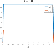
Let and be the total mass of followers and leaders at time , respectively. Since the total mass is preserved, by renormalizing at the initial time, it holds . We assume that at time the initial data is uniformly distributed in with initial density .
We report in Table 1 the model parameters for two different test cases. In both cases, we assume that leaders have larger range of influence than followers, with and . For the numerical discretization, we select space grid points, time step and final time .
| Test | ||||||||
|---|---|---|---|---|---|---|---|---|
| Ia | 0.2 | 0.6 | 0.1 | 0.95 | 0.75 | 0.25 | – | – |
| Ib | 0.2 | 0.6 | (86) | (87) | 0.75 | 0.25 | 0.35 | 0.2 |
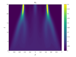
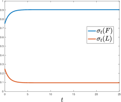
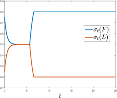
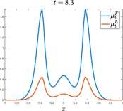
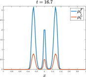
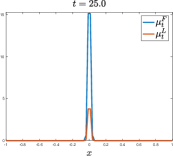
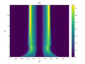
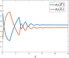
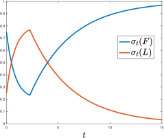
Test Ia: constant rates. We have reported in Figure 1 the evolution of the mean-field system with different simulations, when constant transition rates are selected. According to Table 1, we selected . Notice that in the case of constant rates the total masses converge to
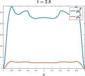
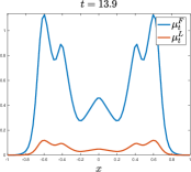
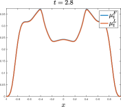
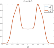
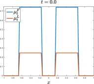
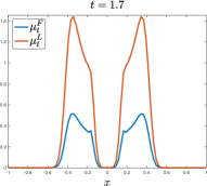
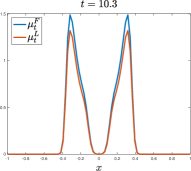
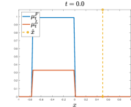
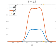
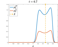
Figure 1 depicts the density in the time interval , and the time evolution of and . In Figure 2 we report different time frame of the densities . We observe that at final time the system has clustered around three states.

Test Ib: Density-dependent rates. We consider birth rates depending on the densities . We consider the variance measure of defined as follows
| (85) |
which measures the spread of the solution over . The birth rate of leaders is selected as a switching function with respect to the dispersion measure (85), such that creation is activated only when the dispersion is above a certain threshold . Thus, we consider the following Lipschitz approximation of the indicator function
| (86) |
with , here we select , and .
Note that function (85) is exactly of the form (94), with . At the same time equation (86) complies with Assumption (H5), as shown in A, as long as for a fixed threshold . This last condition can be easily checked along the evolution.
The creation of followers given by rate is instead determined by the following switching function
| (87) |
namely when the total mass of leaders is above a threshold . Here we selected , and .
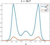
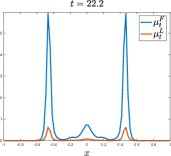
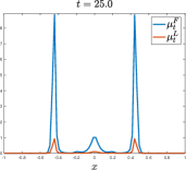
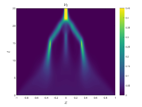
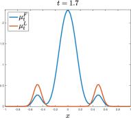
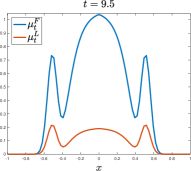
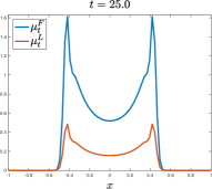
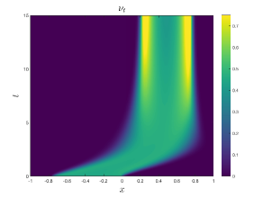
Similarly to the previous test, we show in Figure 3 the total density on and the time evolution of and . In this case we observe the emergence of a consensus state before final time . This is explained by the large amount of leaders, whose mass increases until the total mass is too spread over the domain (and so the measure is above the threshold ). As soon as the threshold is reached, the creation of leaders is stopped and converge to an asymptotic state thanks to the concentration of the total mass. In Figure 4 we show some frames of the time evolution of .
5.2. Test II: Aggregation dynamics
We consider an aggregation dynamics ruled by an attraction towards the population of leaders, and repulsion towards the followers. Hence, we assume the following interaction kernels
with non-negative parameters and .
The exchange of mass between leaders and followers is described as follows: we consider a constant rate , whereas leaders’ birth rate depends non-linearly on the followers’ density. Similarly to Test I we use the variance measure (85) for as follows
| (88) |
The birth rate is the switching function (86), modified as follows
| (89) |
with and . Hence, we expect the total mass of leaders to increase when the followers’ density is too spread over the domain , and to decrease when followers’ density is sufficiently concentrated.
Note that this choice controls the competition between the repulsive action of followers’ kernel and the attraction of the leaders’ one. In order to show the richness of this setting we consider two different cases. The choice of the parameters are reported in Table 2.
For the numerical solution of the mean-field dynamics we fix the computational domain with zero-flux boundary conditions, discretized with space grid points, and time step and final time .
| Test | ||||||||
|---|---|---|---|---|---|---|---|---|
| IIa | 3 | 0.75 | 0.1 | (89) | 0.15 | 0.25 | 0.75 | 0.25 |
| IIb | 2 | 0.5 | 0.1 | (89) | 0.2 | 0.25 | 0.75 | 0.25 |
Test IIa: Uniform initial data. We consider an initial configuration where leaders and followers occupy the same domain’s portion identified by the function
with and . The initial data of (1) is defined as follows
| (90) |
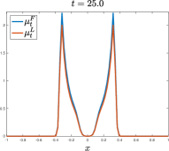
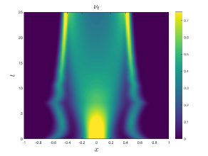
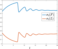
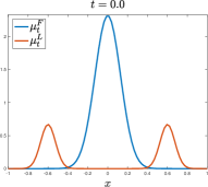
We report in Figure 5 the evolution of the system, observing an oscillating behavior of the total mass of leaders and followers towards a stable configuration of the densities’ profiles. Indeed, initially the density of leaders increases to balance the spread of the initial mass (90), up to the moment when the birth rate is switched off. Subsequently, the mass of followers starts to increase, together with the intensity of the repulsion force. Therefore, the dispersion measure (88) increases again, until the reactivation of the birth rate function . At final time , the system has reached a stationary configuration of the densities as well as of the total masses .
Test IIb: Confinement. We consider a confinement setting, where the leaders’ density surrounds the initial density of followers. In this particular situation, differently from the previous cases, Assumption (H1) on the initial data is not plausible anymore, therefore we renounce to it. We however recall the reader that an existence and uniqueness theory for system (1) is still available, since Propositions 3.2 and 3.3 do not require (H1) to be fulfilled.
We introduce the Gaussian function
then we define the initial data as follows
In this setting, the initial dispersion of followers is not large enough to activate the birth rate , (89). Indeed we can observe from the first two frames of Figure 6-bottom row that the density of followers starts to grow on the support of , while the creation of leaders is not inhibited. In a second step, when the interaction becomes too repulsive, the spread of activates the creation of leaders, and eventually stabilizes the total density towards a stable configuration, with the masses converging towards a stationary value.
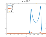
5.3. Test III: Leaders with steering action
We study a population of leaders aiming to reach a desired position , and how their motion influences the followers’ density. The followers’ dynamics is governed by an aggregation equation of the type
Leaders have a steering drift towards of the form
which also complies with our abstract framework, as discussed in Remark 3.6.
We choose a constant rate for the death of leaders , and the following state-dependent rate for the birth of leaders
| (91) |
with , and where is the variance of followers’ density with respect to the desired configuration ,
Hence, we expect the leaders’ density to increase when followers are not concentrated around , and to vanish as soon as the desired state is approached.
This test case is inspired by applications in pedestrian dynamics, where a part of the total mass of agents (leaders) is used as control variable to improve the evacuation time of a crowd [2, 16]. We remain in a simplified setting: similarly to the previous tests, we solve numerically the evolution of the mean-field interaction dynamics in the one-dimensional domain with zero-flux boundary conditions. For the numerical discretization we select space grid points, time step and final time . We have reported in Table 2 the parameters’ choice for the different cases.
| Test | ||||||||||
|---|---|---|---|---|---|---|---|---|---|---|
| III | 2 | 1 | 0.05 | 0.0001 | (91) | 0.15 | 0.25 | 0.75 | 0.25 | 0.5 |
Figure 7 shows the evolution of the density and the evolution of the followers’ and leaders’ masses in the top row. Bottom row shows the evolutions of : the mass of leaders increases initially since followers are far away from , as soon as approaches , while the density of leaders tends to vanish.
Acknowledgments
This work has been supported by the INdAM-GNCS 2018 project Numerical methods for multiscale control problems, and the project “MIUR Departments of Excellence 2018-2022”.
Appendix A Examples of transition functionals
We prove a simple sufficient condition for and to satisfy (H5).
Proposition A.1.
For , let be given locally Lipschitz continuous functions and consider a locally Lipschitz function . Then the map
satisfies Assumption (H5).
Proof.
By possibly arguing componentwise on the ’s we can only consider the case . For all , satisfying , and with support contained in , we clearly have
With this hypothesis, since the function is Lipschitz, it only suffices to show that the functions
satisfy (H5). We only discuss the second case, since the proof in the other cases is similar.
Denote with the function defined by . Whenever has support contained in and satisfies we clearly have
| (92) |
A direct computation also shows that, if we denote with the Lipschitz constant on a ball of radius , it holds
| (93) |
Take now and positive measures satisfying (23) and (24). Use (92) and (93), toghether with the Kantorovich-Rubinstein duality, we have
with . This concludes the proof. ∎
Example A.2.
The statement above is clearly still valid if only depends on some of the variables indicated above. In some applications (as for instance in [27]) the transition rate behaves countercyclically with respect to the mass of : whenever is below a certain threshold , the function increases in order to restore to higher levels. To model this phenomenon, let be a mollification of the function
with . Then, by Proposition A.1 (with for and ) the function satisfies Assumption (H5).
Also quotients of functions of the type considered in Proposition A.1 are easily seen to comply with Assumption (H5), provided that the denominator is bounded away from zero. For instance, for a given scalar-valued and , where is a fixed threshold, one can consider a function of the type
| (94) |
If , and we set , then the above function reduces to
which, as long as , coincides with and only takes into account the total distribution of the two populations.
Appendix B Finite-volume scheme for mean-field leader-follower dynamics
We introduce a finite-volume scheme for the discretization of the mean-field system (1) in one-space dimension. Hence we consider a constant discretization step , and we define with , and the cells , with , over which we define the averages
where we used the notation for the measure . In the same spirt we define the numerical fluxes as follows
In what follows we will consider an upwinding scheme, where the convolutional operator is evaluated at the interfaces according to quadrature formula, and the densities are defined as follows
The sources terms are computed by averaging the transition rates , as follows
We employ a first-order time marching scheme to compute the solution over the time grid , with fixed time step . Moreover we used a splitting technique to evaluate separately the contribution by the non-linear transport and the source terms. Thus the full discrete scheme reads
References
- [1] S. Ahn, H.-O. Bae, S.-Y. Ha, Y. Kim, and H. Lim. Application of flocking mechanism to the modeling of stochastic volatility. Math. Models Methods Appl. Sci., 23(9):1603–1628, 2013.
- [2] G. Albi, M. Bongini, E. Cristiani, and D. Kalise. Invisible control of self-organizing agents leaving unknown environments. SIAM J. Appl. Math., 76(4):1683–1710, 2016.
- [3] G. Albi, Y.-P. Choi, M. Fornasier, and D. Kalise. Mean field control hierarchy. Applied Mathematics & Optimization, 76(1):93–135, 2017.
- [4] G. Albi, L. Pareschi, and M. Zanella. Boltzmann-type control of opinion consensus through leaders. Phil. Trans. R. Soc. A, 372(2028):20140138, 2014.
- [5] G. Albi, L. Pareschi, and M. Zanella. Opinion dynamics over complex networks: Kinetic modelling and numerical methods. Kinetic & Related Models, 10(1):1–32, 2017.
- [6] L. Ambrosio and W. Gangbo. Hamiltonian ODEs in the Wasserstein space of probability measures. Comm. Pure Appl. Math., 61(1):18–53, 2008.
- [7] L. Ambrosio, N. Gigli, and G. Savaré. Gradient Flows in Metric Spaces and in the Space of Probability Measures. Lectures in Mathematics ETH Zürich. Birkhäuser Verlag, Basel, 2008.
- [8] P. Bak. How nature works: the science of self-organized criticality. Springer Science & Business Media, 2013.
- [9] M. Ballerini, N. Cabibbo, R. Candelier, et al. Interaction ruling animal collective behavior depends on topological rather than metric distance: Evidence from a field study. P. Natl. Acad. Sci. USA, 105(4):1232–1237, 2008.
- [10] R. Bellman. Dynamic programming. Princeton University Press, 1957.
- [11] N. Bellomo and C. Dogbe. On the modeling of traffic and crowds: a survey of models, speculations, and perspectives. SIAM Rev., 53(3):409–463, 2011.
- [12] M. Bongini and G. Buttazzo. Optimal control problems in transport dynamics. Math. Models Methods Appl. Sci., 27(3):427–451, 2017.
- [13] M. Bongini and M. Fornasier. Sparse control of multiagent systems. In Active Particles, Volume 1, pages 259–298. Springer, 2017.
- [14] M. Bongini, M. Fornasier, M. Hansen, and M. Maggioni. Inferring interaction rules from observations of evolutive systems I: The variational approach. Math. Models. Meth. Appl. Sci., 27(05):909–951, 2017.
- [15] M. Bongini, M. Fornasier, F. Rossi, and F. Solombrino. Mean-field Pontryagin maximum principle. J. Optim. Theory Appl., 175(1):1–38, 2017.
- [16] M. Burger, M. Di Francesco, P. A. Markowich, and M.-T. Wolfram. Mean field games with nonlinear mobilities in pedestrian dynamics. Discrete & Continuous Dynamical Systems-B, 19(5):1311–1333, 2014.
- [17] J. A. Carrillo, Y.-P. Choi, and M. Hauray. The derivation of swarming models: mean-field limit and wasserstein distances. In Collective dynamics from bacteria to crowds, pages 1–46. Springer, 2014.
- [18] J. A. Carrillo, Y.-P. Choi, and S. P. Perez. A review on attractive–repulsive hydrodynamics for consensus in collective behavior. In Active Particles, Volume 1, pages 173–228. Springer, 2017.
- [19] J. A. Carrillo, S. Fagioli, F. Santambrogio, and M. Schmidtchen. Splitting schemes and segregation in reaction cross-diffusion systems. SIAM Journal on Mathematical Analysis, 50(5):5695–5718, 2018.
- [20] L. Chizat, G. Peyré, B. Schmitzer, and F.-X. Vialard. An interpolating distance between optimal transport and fisher–rao metrics. Foundations of Computational Mathematics, 18(1):1–44, 2018.
- [21] M. Cirant. Multi-population mean field games systems with Neumann boundary conditions. Journal de Mathématiques Pures et Appliquées, 103(5):1294–1315, 2015.
- [22] S. Cordier, L. Pareschi, and G. Toscani. On a kinetic model for a simple market economy. J. Stat. Phys., 120(1-2):253–277, 2005.
- [23] E. Cristiani, B. Piccoli, and A. Tosin. Multiscale modeling of pedestrian dynamics, volume 12. Springer, 2014.
- [24] R. Dobrushin. Vlasov equations. Funct. Anal. Appl., 13(2):115–123, 1979.
- [25] M. Dorigo and C. Blum. Ant colony optimization theory: A survey. Theoretical computer science, 344(2-3):243–278, 2005.
- [26] R. M. Dudley. Real Analysis and Probability. Chapman and Hall/CRC, 1989.
- [27] B. Düring, P. Markowich, J.-F. Pietschmann, and M.-T. Wolfram. Boltzmann and Fokker–Planck equations modelling opinion formation in the presence of strong leaders. Proc. R. Soc. Lond. Ser. A Math. Phys. Eng. Sci., 465(2112):3687–3708, 2009.
- [28] A. F. Filippov. Differential Equations with Discontinuous Righthand Sides. Kluwer Academic Publishers, 1988.
- [29] M. Fornasier, B. Piccoli, and F. Rossi. Mean-field sparse optimal control. Philos. Trans. R. Soc. Lond. Ser. A Math. Phys. Eng. Sci., 372(2028):20130400, 2014.
- [30] M. Fornasier and F. Solombrino. Mean-field optimal control. ESAIM Control Optim. Calc. Var., 20(4):1123–1152, 2014.
- [31] N. Fournier and A. Guillin. On the rate of convergence in Wasserstein distance of the empirical measure. Probab. Theory Related Fields, 162(3-4):707–738, 2015.
- [32] A. Garroni, P. van Meurs, M. A. Peletier, and L. Scardia. Convergence and non-convergence of many-particle evolutions with multiple signs. arXiv preprint arXiv:1810.04934, 2018.
- [33] F. Golse. The mean-field limit for the dynamics of large particle systems. In Journées “Équations aux dérivées partielles”, Forges-les-Eaux, France, 2 au 6 juin 2003. Exposés Nos. I-XV, pages 1–47. Nantes: Université de Nantes, 2003.
- [34] R. Hegselmann and U. Krause. Opinion dynamics and bounded confidence models, analysis, and simulation. J. Artif. Soc. Soc. Simulat., 5(3), 2002.
- [35] H. Huang, J.-G. Liu, and J. Lu. Learning interacting particle systems: Diffusion parameter estimation for aggregation equations. Mathematical Models and Methods in Applied Sciences, to appear, 2018.
- [36] J. Kennedy. Particle swarm optimization. In Encyclopedia of machine learning, pages 760–766. Springer, 2011.
- [37] S. Kondratyev, L. Monsaingeon, and D. Vorotnikov. A new optimal transport distance on the space of finite Radon measures. Adv. Differential Equations, 21(11-12):1117–1164, 2016.
- [38] J.-M. Lasry and P.-L. Lions. Mean field games. Jpn. J. Math., 2(1):229–260, 2007.
- [39] M. Liero, A. Mielke, and G. Savaré. Optimal transport in competition with reaction: the Hellinger-Kantorovich distance and geodesic curves. SIAM J. Math. Anal., 48(4):2869–2911, 2016.
- [40] H. P. McKean. Propagation of chaos for a class of non-linear parabolic equations. Lecture Series in Differential Equations, Catholic University, Washington D.C., 7:41–57, 1967.
- [41] S. Méléard. Asymptotic behaviour of some interacting particle systems; McKean-Vlasov and Boltzmann models. In Probabilistic models for nonlinear partial differential equations (Montecatini Terme, 1995), volume 1627 of Lecture Notes in Math., pages 42–95. Springer, Berlin, 1996.
- [42] B. Piccoli and F. Rossi. Transport equation with nonlocal velocity in Wasserstein spaces: Convergence of numerical schemes. Acta Appl. Math., 124(1):73–105, 2013.
- [43] B. Piccoli and F. Rossi. Generalized Wasserstein distance and its application to transport equations with source. Arch. Ration. Mech. Anal., 211(1):335–358, 2014.
- [44] B. Piccoli and F. Rossi. On properties of the generalized Wasserstein distance. Arch. Ration. Mech. Anal., 222(3):1339–1365, 2016.
- [45] B. Piccoli and F. Rossi. Measure-theoretic models for crowd dynamics. In Crowd Dynamics Volume 1 - Theory, Models, and Safety Problems. N. Bellomo and L. Gibelli Eds, Birkhauser, to appear.
- [46] A.-S. Sznitman. Topics in propagation of chaos. In École d’Été de Probabilités de Saint-Flour XIX—1989, volume 1464 of Lecture Notes in Math., pages 165–251. Springer, Berlin, 1991.
- [47] M.-N. Thai. Birth and death process in mean field type interaction. Bernoulli, to appear, 2018.
- [48] T. Vicsek and A. Zafeiris. Collective motion. Phys. Rep., 517(3):71–140, 2012.
- [49] C. Villani. Topics in Optimal Transportation, volume 58 of Graduate Studies in Mathematics. American Mathematical Society, Providence, RI, 2003.