PREPERIHELION OUTBURSTS AND DISINTEGRATION OF COMET C/2017 S3 (PAN-STARRS)

Abstract

A sequence of events, dominated by two outbursts and ending with the preperihelion disintegration of comet C/2017 S3, is examined. The onset times of the outbursts are determined with high accuracy from the light curve of the nuclear condensation before it disappeared following the second outburst. While the brightness of the condensation was declining precipitously, the total brightness continued to grow in the STEREO-A’s HI1 images until two days before perihelion. The red magnitudes measured in these images refer to a uniform cloud of nuclear fragments, 2200 km² in projected area, that began to expand at a rate of 76 m s^-1 at the time of the second outburst. A tail extension, detected in some STEREO-A images, consisted of dust released far from the Sun. Orbital analysis of the ground-based observations shows that the comet had arrived from the Oort Cloud in a gravitational orbit. Treating positional residuals as offsets of a companion of a split comet, we confirm the existence of the cloud of radiation-pressure driven millimeter-sized dust grains emanating from the nucleus during the second outburst. We detect a similar, but compact and much fainter cloud (or a sizable fluffy dust aggregate fragment) released at the time of the first outburst. — The debris would make a sphere of 140 m across and its kinetic energy is equivalent to the heat of crystallization liberated by 10⁸ g of amorphous water ice. Ramifications for short-lived companions of the split comets and for 1I/‘Oumuamua are discussed.

1. Comet’s Discovery and Early Behavior

The discovery of comet C/2017 S3 was reported jointly by R. J. Wainscoat and R. Weryk to result from systematically surveying the sky with the Pan-STARRS 1 180-cm f/4.4 Ritchey-Chrétien telescope at Haleakalā, Hawaii, on 2017 September 23; prediscovery images of the comet were subsequently identified in several exposures taken on August 17 and September 7 (Green 2017). At the time of discovery, the object was of magnitude 21, not stellar in appearance, and showing possible asymmetry to the east. The preliminary orbit (Williams 2017a, 2017b) was still too uncertain to reveal the object’s origin, but a subsequent orbit determination that linked about 50 astrometric observations over a period of three months, from August 17 to November 18 (Nakano 2018a), already left no doubt that C/2017 S3 was a dynamically new comet that had arrived from the Oort Cloud. These computations also implied that the comet was near 5 AU from both the Sun and the Earth when discovered, that it was on its way to perihelion at 0.21 AU from the Sun, to arrive shortly before 2018 August 16.0 UT, and that the orbital plane had an inclination of 99^∘ to the plane of the ecliptic.

The comet was an unimpressive object at heliocentric distances greater than 1.3 AU before perihelion, and few physical observations are available from that period of time. Between 2.3 AU and 1.4 AU from the Sun, the comet’s total brightness corrected for the phase effect, normalized to 1 AU from the Earth, and after personal and instrumental corrections have been applied, was found to have varied with heliocentric distance, $r$, according to a power law $r^{-n}$, where $n=3.0$ $\pm$ 0.5, close to Whipple’s (1978) average for Oort Cloud comets before perihelion; the “absolute” magnitude (normalized to 1 AU from the Sun) amounted to $H_{0}=10.7$ $\pm$ 0.3, which made the comet a likely candidate for imminent disintegration (Section 4.2).

As late as the second half of June 2018, only 7–8 weeks before perihelion, the comet looked like a faint speck of light, never reported brighter than magnitude 13. Moreover, scattered values of a dust-production rate proxy parameter Af$\rho$ from late June (see footnote 1) clustered in a range of 50–55 cm, implying an object depleted in dust, in line with the essentially spherical coma, hardly any dust tail at all, and additional evidence that is presented below. In summary, a lackluster performance.

And then it happened: As June was making way for July, the comet exploded dramatically, rapidly developing a sharp, brilliant nuclear condensation and finding itself all of a sudden at the life’s crossroads. Its fate was about to be sealed in the next few weeks.

2. Phenomenon of Cometary Outburst

With the advent of space exploration, cometary activity has been recognized to consist of contributions from a number of discrete sources on and beneath the surface of the nucleus, whose emission rates vary with time, depending on their composition, morphology, dimensions, and the solar energy input received. As a function of the orbit, the nucleus’ shape, rotation, and other properties, the comet’s light curve is always complex, with frequent short-term ups and downs. From time to time, a major subsurface reservoir of ices is activated, leading to a sudden surge in brightness — an event that is referred to as an outburst.

With no universally accepted definition, we follow here the description proposed by Sekanina (2010), according to which an outburst is any sudden, prominent, and unexpected brightening, caused by an abrupt short-term injection of massive amounts of volatile material from the nucleus into the atmosphere. The fundamental parameters that describe an outburst in a comet’s light curve are: (i) the time of onset, (ii) the brightness at the peak, (iii) the rise time (between the onset and the peak), and (iv) the amplitude (the increase in brightness from the onset to the peak). Also critital is the degree of asymmetry between the event’s rising and subsiding branches. The rise time can be as short as a fraction of a day and very seldom exceeds a few days. The amplitude should equal at least 0.8–1.0 mag, equivalent to a flux increase by a factor of 2 to 2.5, but is usually a few magnitudes. The more appropriate parameters from the standpoint of outburst physics are described elsewhere (Sekanina 2017), together with analysis of the photometric data for 20 selected events experienced by 10 comets.

Cometary outbursts are frequent and very diverse phenomena, which can be categorized from various points of view. In regard of C/2017 S3, we mention two major criteria: one is the overall temporal profile, which separates gas-dominated from dust-dominated outbursts; the other criterion is the degree of repercussions for the comet’s post-event evolution, which divides the outbursts into innocuous and ominous (or portentous) and subdivides the latter into nonfatal and cataclysmic.

The main difference between the gas-dominated and dust-dominated outbursts is the degree of asymmetry between the rising and subsiding branches. Gas-dominated events are nearly symmetric relative to the peak, particularly at smaller heliocentric distances, because the subsiding branch reflects the fairly short photodissociation lifetime of the molecular species, primarily diatomic carbon, observed in the light curve. The subsiding branch of dust-dominated events is much more extended because it is determined by the residence time of dust grains in the coma, which, for larger particles in particular, is considerably longer than the dissociation lifetime of molecules. Accordingly, dust-dominated outbursts are highly asymmetric with respect to the peak.

Having experienced an innocuous outburst, the comet does not subsequently exhibit any anomalous changes in its behavior, the post-event activity pattern resembling the pre-event one. By contrast, a nonfatal outburst leaves a mark on the comet’s activity and/or appearance. Following the event, the comet may stay intrinsically either much brighter or much fainter over extended periods of time. A more vigorous effect of a nonfatal outburst is its intimate association with — or, rather, a de facto manifestation of — a splitting of the nucleus into two or more massive fragments. Some time after the outburst subsides, the comet’s nucleus begins to appear double or multiple, with the separation increasing with time. Its further evolution varies from case to case, but typically only the primary fragment survives with no signs of deteriorating health. In a cataclysmic outburst the comet’s existence is terminated by complete — whether rapid or more gradual — disintegration into refractory debris; following the peak, the brightness of the comet’s near-nucleus region plunges precipitously never to recover again. Accordingly, this type of outburst could also be referred to as terminal.

Outbursts are not necessarily isolated events, as they sometimes come in pairs or larger lineups, separated by relatively short periods of time. The individual events in a group of outbursts could be either of the same category in terms of the repercussions (e.g., two consecutive nonfatal outbursts accompanying two nucleus fragmentation events) or of different categories (e.g., an innocuous outburst followed by a cataclysmic outburst). Regrettably, one cannot distinguish whether an outburst is innocuous or ominous until the repercussions become evident. Accordingly, an unfortunate property of outbursts is that they cannot serve as ground for prognosticating the comet’s future health.

3. Continuing Saga of Comet C/2017 S3

The comet’s explosion, referred to at the end of Section 1, was the outset of a bona fide outburst, as defined in Section 2. The event was first reported by M. Jäger, who noticed it in an image that he had obtained with a 30-cm f/4 telescope at Stixendorf, Austria (Code A71), on July 1.98 UT. The comet was then 3 mag brighter than the previous day. From the temporal variations in the Af$\rho$ parameter and in the nuclear magnitudes of the comet, E. Bryssinck pointed out that the event began on June 30. On July 4.0 UT, Jäger detected a 10^′ long ion tail. The nuclear condensation was brightening according to him until July 4, which is consistent with A. Novichonok’s estimates of the total magnitude. The brightness then began to subside and by July 13, the nuclear condensation became indistinct to the extent that Jäger suspected the comet’s disintegration in progress.

However, on July 15.0 UT a second outburst was in full bloom, the comet described by Jäger as strongly condensed and an ion tail apparent. The brightness in an aperture of 40^′′ across was seven times higher than in an aperture of 12^′′, suggesting a relatively flat distribution of the surface brightness, decreasing with the distance $\rho$ from the center only as $\rho^{-0.4}$. M. Meyer noticed on July 20 that the comet was losing the condensation, a development reminiscent of the first outburst. The appearance of the ion tail was intermittent; for example, it was prominent and nearly 3^∘ long in an image taken by G. Rhemann, Eichgraben, Austria (Code C14), on July 20.0 UT, but was completely missing in his image taken 23 hours later. J.-F. Soulier, observing with a 30-cm f/3.8 reflector at Maisoncelles, France (Code C10), said that in an image taken on July 27.06 UT the comet appeared to be “in agony”, while Jäger’s animation using his images taken on August 1 showed the comet’s head diffuse and clearly elongated. The last ground-based observation was made by Soulier on August 3, when the comet’s elongation from the Sun was 27${}^{\circ}\!$.3; it dropped to 25^∘ in the next 24 hours.

Figure 1.— Light curve of the nuclear condensation of comet C/2017 S3, based on 129 averages of 525 individual nuclear-magnitude determinations by 15 observers. The data were normalized to 1 AU from the Earth and a 4^′′ aperture and corrected for instrumental effects and for the phase effect with the Marcus (2007) law for dust-poor comets. After a gradual brightening, Outburst I began 46.8 days before perihelion at 1.25 AU from the Sun, Outburst II 32.6 days before perihelion at 0.96 AU from the Sun. The rise time and amplitude equal, respectively, 4 days and 2.5 mag for Outburst I and 1.5 days and 3.2 mag for Outburst II. The prominent, rapid post-peak fading is typical of gas-dominated outbursts. Note the steep terminal rate of decline at $\sim$0.3 mag per day. The perihelion occurred on 2018 August 15.95 TT.

It was fortunate that on July 31 the comet entered the field of view of the HI1 imager of the STEREO-A spacecraft, in which it stayed until August 14. The comet was easily seen in the level-2 images, which we examined.

More than a week after perihelion, the comet began to transit the field of view of the C3 coronagraph on board the SOHO spacecraft. Our inspection of these images failed to show any trace of the comet.

In the light of this, a report of visual detection of the comet’s debris 2–3 months after perihelion was rather unexpected. The recovery remained unconfirmed, as independent searches failed to corroborate the report.

The comet’s apparent demise soon after the two outbursts poses questions on their possible impact, such as: Which outburst was more damaging to the comet’s nucleus? Or: Would the effects of the second event be less severe in the absence of the first? We address these and related issues (i) by studying the changes in the brightness and appearance of the comet with time, and (ii) by investigating its orbital motion.

4. The Light Curve

This section is divided into three parts to accentuate the differences in the photomteric behavior of the nuclear condensation and the comet as a whole, as well as to underline the apparent correspondence between the ground-based and STEREO-A light curves.

4.1. CCD Nuclear Magnitudes

It was proposed in Sekanina (2010) that, if properly analyzed, CCD nuclear magnitudes routinely reported with astrometric observations in the publications of the IAU Minor Planet Center (MPC) can be used to constrain, often very tightly, the onset time of outbursts. Because of equipment differences among the observers (especially in the size of the scanning aperture and the filter used), appropriate corrections should be applied before the data sets are combined and the method allowed to work.

Employing this technique, we utilized 129 averages of 525 individual rapid-succession observations of the nuclear magnitude (marked by N), as well as color data — G, R or V — if comparable to N, obtained at 15 observing sites (Codes 970, A71, A77, B96, C10, C23, C47, D35, G40, J01, J22, J95, K02, L12, Z80). Very few data were discarded because of their sizable deviations from the remarkably consistent curve presented in Figure 1, in which the nuclear magnitudes are normalized to 1 AU from the Earth and are corrected for the phase effect using the Marcus (2007) law for dust-poor comets. Rather arbitrarily, the instrumental corrections were applied to reduce the data to Jäger’s magnitude scale for a scanning aperture of 4^′′ in radius.

Figure 2.— Light curve of comet C/2017 S3 based on the total visual and CCD observations from the ground (solid circles) and measured by the second author from level-2 images taken with the HI1 imager on board STEREO-A (circled dots). The plotted magnitudes $H_{\Delta}$ were normalized and corrected in the same fashion as the nuclear magnitudes in Figure 1. While both light curves show the two outbursts, they differ from one another dramatically after Outburst II terminated, when the total brightness began to increase again. There is also possible evidence for a precursor flare-up prior to Outburst I. The measured R magnitudes of the STEREO-A images were converted from the R to V magnitudes by applying an approximate color index of +0.4 mag. The perihelion occurred on 2019 August 15.95 TT.

The outbursts differ from one another in several respects. Both the rising and subsiding branches for the second outburst are distinctly steeper and its amplitude is higher (3.2 mag against 2.5 mag) than for the first outburst. The peak of the second outburst appears to be distinctly wider, suggesting perhaps that the event consisted of several explosions in rapid succession. The steep subsiding branches are strong evidence that both outbursts were unquestionably gas-dominated events. And the steeper slope of the second outburst may imply an effect of the lifetime of molecules, which varies with the square of heliocentric distance. The rate of fading after the second outburst was brutal, $\sim$0.3 mag per day, an indication that the nuclear region was being very thoroughly vacated by gas and photometrically effective dust. However, one cannot rule out that sizable inactive fragments, which are difficult to detect, still persisted near the location of the parent nucleus.

The first outburst must have begun many hours before July 1.0 UT, because three observers reported the comet to have already been anomalously bright, displaying a brilliant, starlike nuclear condensation, around the UT midnight from the 30th to the 1st. These and other observations made between July 1.0 and 3.0 UT line up in the plot of the light curve along a slope implying that the event commenced close to June 30.0 UT, except that the images by A. Diepvens with a 20-cm refractor at Olmen, Belgium (Code C23), preclude an onset time before June 30.1 UT. These constraints provide for the nominal time of onset for this Outburst I an estimate of June 30.2 $\pm$ 0.1 UT.

Similarly, the second outburst could not commence after July 14.9 UT because it was already in progress three quarters of an hour before the UT midnight of July 15, when Soulier took the first image of the night. The flare-up was confirmed a half an hour later, still before the midnight, by P. Carson’s observations at the Eastwood Observatory (Code K02), Leigh-on-Sea, Essex, United Kingdom, with a 32-cm reflector and f/5.4 focal reducer; and within minutes of the midnight by other observers, including G. Dangl at Nonndorf, Austria (Code C47), G. Vandenbulcke at Koksijde, Belgium (Code L12), as well as Bryssinck and Jäger. On the other hand, the observations by B. Lütkenhöner et al. at the Slooh Observatory on Mt. Teide, Tenerife, Canary Islands (Code G40), and by K. Hills, who worked with a 50-cm f/2.9 astrograph at the Tacande Observatory, La Palma, Canary Islands (Code J22), rule out an onset before July 14.3 UT. We adopt July 14.4 $\pm$ 0.1 UT as the start of Outburst II.

4.2. Total Magnitudes from Ground-Based Observations, and the Comet’s Appearance

We were able to collect ground-based observations of the comet’s total brightness made by 20 observers. Most of the data come from 14 visual observers, who reported their results either to the Crni Vrh Observatory’s COBS Database, or to the International Comet Quarterly, the two sources we consulted to collect the data for analysis. However, because the comet had been very faint before undergoing the first ourburst, it was necessary to supplement the visual observations with a set of total CCD magnitudes. Most of these data were obtained from the Minor Planet Center’s database of astrometric observations (see footnote 5), the source that also provided the large set of nuclear magnitudes. Additional total CCD magnitudes were found in the two sources of visual magnitudes.

Although combining visual and CCD magnitudes carries risks of their questionable compatibility, we used the method, expounded in some detail elsewhere (Sekanina 2017), that applies appropriate personal and instrumental corrections to minimize these risks. Since information on the comet’s brightness at very large heliocentric distances was too fragmentary, we limited our analysis to an orbital arc of less than $\sim$100 days from perihelion. The compatibility tests were passed by the data sets reported by only seven CCD observers.

Figure 3.— Variations in the total normalized brightness of the comet C/2017 S3 as a function of heliocentric distance. The magnitudes $H_{\Delta}$ are identical with those in Figure 2. The comet’s pre-outburst gradual brightening at distances exceeding 1.4 AU from the Sun preperihelion is shown at the lower left. The extrapolated absolute magnitude $H_{0}$ and the onset points, Onset(I), Onset(II), and the peak points, Peak(I), Peak(II), of the two outbursts are depicted. Selected total magnitudes from the level-2 images by the HI1 camera on board STEREO-A, displayed to the upper right, are the same data as in Figure 2. The comet’s perihelion distance of 0.208 AU is marked by $\Pi$.

The total number of ground-based observations, either visual or CCD, employed in our analysis and plotted in Figure 2, is 109. All 11 data points beyond 1.4 AU from the Sun are CCD magnitudes. The scatter among the total brightness entries is greater than that among the nuclear magnitudes and it is estimated at $\pm$0.3 mag on the average. The main problem with the total CCD magnitudes is is that they often exclude the outermost coma and require large corrections to account for this deficit.

The light curve in Figure 2 shows a very gradual brightening of the comet when it was more than 55 days before perihelion or $>$1.4 AU from the Sun. Plotted in Figure 3 against heliocetric distance $r$ rather than time, the normalized brightness varies as $r^{-3.04\pm 0.48}$, a rate that is rather typical of Oort Cloud comets, as already noted in Section 1. The visual absolute magnitude, which characterizes the comet’s stamina, is — when extrapolated from the pre-outburst orbital arc between 2.2 AU and 1.4 AU from the Sun — equal to $H_{0}=10.66\pm 0.32$, more than 2 mag below Bortle’s (1991) perihelion-survival limit (of 8.2 for this object) that identifies objects prone to early disintegration. The subsequent evolution of C/2017 S3, while unpredictable in detail, was not entirely surprising. One unexpected minor feature in the light curve in Figure 2 is a possible precursor flare-up, with an amplitude slightly exceeding 1 mag, which, if genuine, began about 54 days before perihelion, on June 23. This feature does not show up in Figure 1.

The profiles of the two outbursts, including their rise times and the plateau of Outburst II, look rather alike in Figures 1 and 2. The only slight disparity for Outburst I is its higher amplitude, equaling 3.5 mag (and rivaling Outburst II) in the total light.

The stunning difference between the light curves based on the nuclear and total brightness data is apparent at the end of Outburst II: while the nuclear condensation was fading dramatically, the comet’s total brightness stopped subsiding once the flare-up died down. Unfortunately, the object was by then less than 30^∘ from the Sun and ground-based observations terminated. The subsequent developments could luckily be followed in the images taken by the HI1 camera on board STEREO-A, as described below.

A characteristic property of C/2017 S3 was its prominent green color, repeatedly commented on by observers. The color was undoubtedly a corollary of the comet’s visible spectrum being dominated by the $d^{3}\Pi_{g}\!\rightarrow\!a^{3}\Pi_{u}$ transition of the diatomic carbon molecule, whose strongest (0–0) band is near 517 nm.

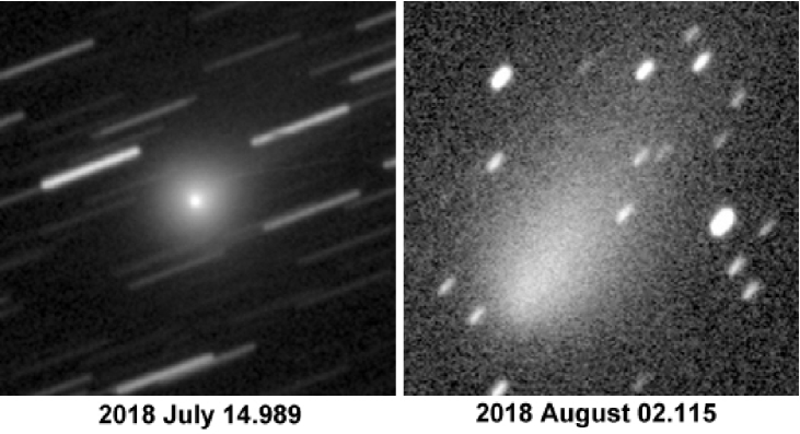
Figure 4.— Comparison of the appearance of C/2017 S3: highly condensed in an early stage of Outburst II (left) and after it permanently lost the nuclear condensation (right). The images were obtained with a 30-cm f/3.8 reflector + CCD (no filter) and each is 4${}^{\prime\!}$.6 on a side. (Image credit: J.-F. Soulier, Maisoncelles, France.)

The appearance of the comet was correlated with its brightness. In the early stage of Outburst I the most striking feature was a bright, starlike nuclear condensation gleaming through the green coma, with ion tail reported on a few occasions, but not continuously. As the outburst proceeded, the condensation was becoming progressively less distinct and more diffuse over a period of several days. At the outset of Outburst II, this cycle of morphological changes repeated itself, but as the event was subsiding, the observers noticed that the condensation continued to expand and fade to the point of disappearance, with the flat surface-brightness distribution in the inner coma somewhat elongated in the antisolar direction, thereby degrading the quality of astrometry.

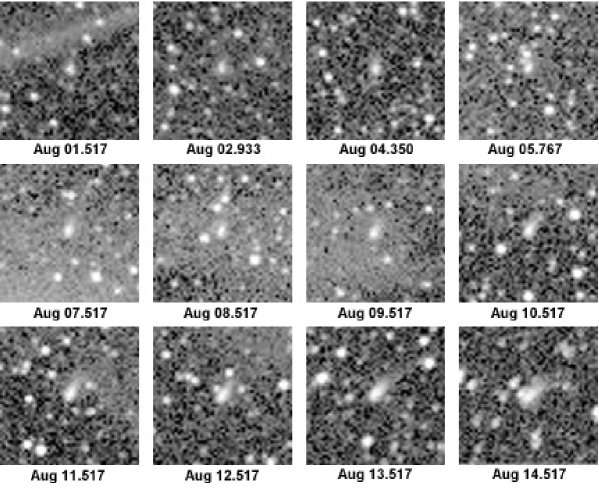
Figure 5.— Examples of the level-2 images of C/2017 S3 taken by the HI1 camera on board the STEREO-A spacecraft on 2018 August 1–14, shortly before perihelion. The cloud of nuclear debris is located in each frame’s center. From August 7 on, a tail is seen to point to the upper right. Each frame is 1^∘ on a side, the position angle of the direction up is $\sim$335^∘. (Image credit: NASA/SECCHI consortium.)

Figure 4 illustrates the contrast between the comet’s appearance soon after the onset of Outburst II and following the disappearance of the nuclear condensaton less than three weeks later.

4.3. Total CCD Magnitudes of the Comet’s Debris
from Images Taken by STEREO-A

By the time the comet entered the field of view of the HI1-A imager, it was clear that the loss of the nuclear condensation was permanent and that the integrity of the comet’s nucleus was compromised, its mass subjected to severe fragmentation. We provide evidence for this conclusion by investigating the comet’s orbital motion in Sections 7–8, but the ground-based imaging from the last days of July and the first days of August leaves no doubt that in late July the object’s ability to function as an active comet was paralyzed and that a cloud of some sort of debris now occupied the position of the former nucleus. To describe the debris is a major goal of this study. We suspect that Outburst II was a cataclysmic event and in the following we search for more supporting evidence.

The comet entered the field of view of the HI1 imager on board STEREO-A on July 31 and left it on August 14. The second author used the Astrometrica interactive software tool to determine magnitudes of the comet’s debris clearly visible in the level-2 images, examples of which are displayed in Figure 5. The measurements were made with a scanning aperture of 2 pixels in radius. With a pixel size of $\sim$72^′′ and the detector’s spectral bandpass of $\sim$600 nm to $\sim$750 nm, the measured data represent total red magnitudes. Their mean error is about $\pm$0.1 mag, substantially better than the uncertainty of the ground-based brightness estimates. Converted to the visual magnitudes by applying an approximate correction of +0.4 mag, they are plotted in Figures 2 and 3. Figure 2 exhibits their excellent compatibility with the ground-based observations; demonstrates, from about July 25 on, an enormous disparity between the light curves derived from, respectively, the nuclear and total brightness (already alluded to in Section 4.2); and indicates that the comet’s debris in the aperture continued to brighten until August 14.0 UT, or 2 days before perihelion. Only at that point did a fading set in.

The most significant piece of information on the brightness evolution of the cloud of debris in Figure 3 is the brightness-variation law of $r^{-2}$ between July 31 and August 7, implying no loss in the projected cross-sectional area of the cloud of fragments in this time span! Regardless of the extent of damage inflicted upon the nucleus, it is obvious that in this period of time the field of debris was still traveling in an organized manner. Excluding an unlikely scenario in which the loss rate of a cross-sectional area is always compensated by the exactly same rate of debris fragmentation, the $r^{-2}$ law suggests that during the week-long period the scanning aperture contained the whole volume of the debris cloud.

Between August 7.0 and 14.0 UT, the comet’s debris still brightened, but at a much slower rate, as $\sim\!\!r^{-\frac{3}{4}}$. In relation to the previous period, this trend can be interpreted to mean that the dimensions of the debris cloud now began to spill outside the field covered by the scanning aperture, with an ever decreasing fraction of the cloud detected. The peak on August 14.0 UT is sharp, the brightness then starting to drop precipitously. This event is deemed to display the last gasp of life, resulting apparently in a rapidly accelerated expansion of a second generation of debris and signaling the imminent, ultimate demise of the comet.

5. Interpretation of the STEREO-A Light Curve

In an effort to model the brightness variations in the STEREO-A images, we formulate a simple hypothesis: at time $t_{\rm frg}$ the comet’s nucleus suddenly disintegrated into a cloud of fragments of equal dimensions, which was optically thin and expanding isotropically with a uniform radial velocity $v_{\rm exp}$, reaching at time $t$ a radius

$$\rho(t)=v_{\rm exp}(t\!-\!t_{\rm frg}).$$ (1)

Let the spatial density of the fragments be independent of the position in the cloud and decreasing with time as $\rho^{-3}$. Centered on a circular scanning aperture $n$ pixels in radius, the cloud stays within the aperture’s bounds as long as

$$\rho\leq a,$$ (2)

where $a$ is the radius of the aperture at the comet’s distance $\Delta$ from the STEREO-A spacecraft,

$$a=725np\Delta,$$ (3)

with $p$ being a pixel size in arcsec, while $\Delta$ is in AU; $a$ is then in km.

As the cloud of debris keeps expanding, its radius is sooner or later bound to exceed the radius of the scanning aperture, $\rho>a$, the volume that stays confined to the aperture is given by the intersection of a cylinder of radius $a$ and infinite length (closely approximating at the comet the scanning cone whose vertex is at the spacecraft) with a sphere, of radius $\rho$, whose center is located on the cylinder’s axis. This confined volume of space equals the sum of the volume of the cylinder of radius $a$ and length 2$b$, where

$$b=\sqrt{\rho^{2}\!-\!a^{2}},$$ (4)

plus the volume occupied by two spherical caps, each having a height $\rho-b$ and a base radius $a$. The volume of the expanding spherical cloud of debris that is confined to the aperture equals

$$U_{\rm apert}=2\pi a^{2}b+\frac{2\pi}{3}(\rho\!-\!b)^{2}(2\rho+b).$$ (5)

Since the total volume of the cloud equals $U_{\rm cloud}=\frac{4}{3}\pi\rho^{3}$, the volume fraction in the scanning aperture amounts to (for $\rho>a$)

$${\cal A}=\frac{U_{\rm apert}}{U_{\rm cloud}}=1-\!\left[1-\!\left(\frac{a}{\rho}\right)^{\!\!2}\right]^{\!\frac{3}{2}}\!\!\!<1,$$ (6)

which is, on our assumptions, also the fraction of the total cross-sectional area of the debris cloud in the aperture’s field. When $\rho\leq a$, the fraction is ${\cal A}=1$.

For the images taken after August 7.0 UT, the expression (6) is to be compared for each imaging time $t$ with the fraction of the cross-sectional area of the debris in the aperture, computed from the absolute magnitude $H_{0}(t)$,

$${\cal A}=10^{0.4(\widehat{H}_{0}-H_{0})},$$ (7)

where $\widehat{H}_{0}$ is the constant absolute magnitude derived from the images taken between July 31 and August 7, representing the total cross-sectional area of the debris in the cloud.

From Equation (6) the radius of the debris cloud equals

$$\rho=a\left[1-(1\!-\!{\cal A})^{\frac{2}{3}}\right]^{-\frac{1}{2}}$$ (8)

and the hypothesis of a uniform isotropic expansion of the debris cloud is tested by its basic condition, expressed by Equation (1). Written as

$$t=t_{\rm frg}+\frac{1}{v_{\rm exp}}\rho,$$ (9)

the two parameters of the hypothesis, the fragmentation time of the debris, $t_{\rm frg}$, and the expansion velocity, $v_{\rm exp}$, are given as the ordinate and the reciprocal of the slope, respectively. The degree, with which the relation approximates a straight line, measures how successful our hypothesis is. Also, if our suspicion that Outburst II was the event that doomed the comet is correct, there should be a correspondence between the fragmentation time $t_{\rm frg}$ and the time of Outburst II.

The measurements of the comet’s apparent red magnitudes in the HI1-A level-2 images were made with a circular aperture of 2 pixels. With a pixel size of 71${}^{\prime\prime\!}$.94, the aperture radius (in km) at the comet’s distance $\Delta$ (in AU) from STEREO-A becomes according to Equation (3) $a=10.43\times\!10^{4}\Delta$.

Table 1 presents the apparent magnitude measurements (in column 3) as a function of time, together with the comet’s distances from STEREO-A and the Sun, the phase angle, and the derived quantities: the absolute red magnitude $H_{0}$, the aperture radius $a$, the fraction of the cross-sectional area of the cloud of debris in the aperture, $\cal A$, derived from Equation (7), and the debris cloud’s radius $\rho$, calculated from Equation (8).

The most striking feature of the first part of the table, July 31.7 to August 7.0 UT, is the essentially constant value of the absolute red magnitude, which averages

$$\widehat{H}_{0}=9.92\pm 0.05.$$ (10)

This absolute magnitude reflects the $r^{-2}$ dependence of the normalized magnitude in Figure 3 and implies a constant cross-sectional area of the fragmented nucleus in the scanning aperture (as noted in Section 4.3), which equals the total cross-sectional area of the cloud, $X_{\rm frg}$. Thus, besides its use in computing the fraction ${\cal A}$ in Table 1 from Equation (7), $\widehat{H}_{0}$ is employed to determine $X_{\rm frg}$ from

$$X_{\rm frg}=\frac{7.03}{p_{\rm R}}10^{16+0.4(\mbox{$\scriptstyle H_{\mbox{\boldmath${\>\!\!\scriptscriptstyle\odot}$}}$}-\widehat{H}_{0})},$$ (11)

where $p_{\rm R}$ is the geometric albedo of the debris in the read part of the spectrum and $H_{\mbox{\boldmath${\scriptstyle\odot}$}}$ is the Sun’s red magnitude. Taking $p_{\rm R}=0.05$ and $H_{\mbox{\boldmath${\scriptstyle\odot}$}}$ = $-$27.10, we find

$$X_{\rm frg}=2200\pm 100\>{\rm km}^{2}.$$ (12)

The hypothesis of a uniform isotropic expansion of the debris cloud is tested in Figure 6, in which the time of observation is plotted as a function of the derived radius of the cloud once it exceeded the radius of the aperture. A least-squares fit to the data in the interval of time August 7.5–13.3 UT yields a solution

$$t\!-\!t_{\pi} = -31.5+1.52\rho,$$

$$\hskip 4.83691pt\pm 2.5\hskip 1.70709pt\pm\!0.15$$

where time is in days, $\rho$ is in 10⁴ km, and $t_{\pi}$ is the comet’s perihelion time derived in Section 7. Figure 6 clearly demonstrates the presence of a linear relationship between $\rho$ and $t$ and submits for the fragmentation time

$$t_{\rm frg}\!-\!t_{\pi}\!=\!-31.5\pm 2.5\;{\rm days}\hskip 8.5359pt(t_{\rm frg}\!=\!{\rm July\,15.5}\pm{\rm 2.5\>UT)},$$ (14)

in excellent conformity with the timing of Outburst II, which according to Figure 1 began 32.6 days before perihelion (July 14.4 UT) and reached a peak 1.5 days later, 31.1 days before perihelion. The cataclysmic nature of Outburst II is hereby strongly supported. From the slope in Equation (13) one gets for the cloud’s expansion velocity before August 14

$$v_{\rm exp}=76\pm 7\;\,{\rm m\,s}^{-1}.$$ (15)

The last four points of Table 1, referring to the measured terminal fading over a period of August 14.0-14.8 UT in Figures 2 and 3, do not fit Equation (13). Instead, they follow a very different straight line of a considerably flatter slope,

$$t\!-\!t_{\pi} = -4.4+0.131\rho,$$

$$\pm 0.2\hskip 1.70709pt\pm\!0.010$$

implying an expansion velocity of 880 $\pm$ 70 m s^-1. We offer no conclusive interpretation of this terminal event, but suggest that it may signal a rapid rate of sublimation of the debris in the cloud, a process that would be consistent with the high expansion velocity.

Figure 6.— Expansion of the cloud of debris after the fragmentation of the nucleus of comet C/2017 S3. Solid circles refer to the times between August 7.0 and 14.0 UT, when the expansion followed Equation (13). The open circles refer to the last four entries in Table 1. The aperture radius is also plotted.

The fit to the cross-sectional area of the fragmented nucleus confined to the scanning aperture, ${\cal A}$, is provided by Equation (6) via Equation (13). It is plotted as a function of time in Figure 7. The fit actually suggests that the scanning aperture was already filled with the fragments by August 5.56 UT, or 10.39 days before perihelion, when the debris cloud expanded to $13.89\times\!10^{4}$ km in radius, which was at the time also the radius of the aperture at the comet’s distance from STEREO-A.

In an effort to further strengthen the case for the debris cloud’s expansion, an obvious avenue was to search for additional evidence among the ground-based imaging observations. Unfortunately, we were able to find no data of this kind. The expansion is surely documented qualitatively beyond a shadow of a doubt by, for example, comparing the two images in Figure 4, but quantitative data are lacking. This may in part be due to the fact that the boundary of the expanding cloud was buried in the coma. The radius $\rho$ in our model thus remains a derived, not measured, quantity. Yet, its introduction in our formulation was a convenient mathematical tool, which was justified by strong evidence from the STEREO-A light curve of the fragmented comet and which allowed us to examine and eventually establish the relationship between the debris and Outburst II.

Figure 7.— Interpretation of the STEREO-A light curve of comet C/2017 S3 in terms of a temporal dependence of the fraction ${\cal A}$ of the cross-sectional area of the fragmented nucleus, detected in the scanning aperture 2${}^{\prime\!}$.4 in radius. The solid circles are the data from Table 1 between July 31.7 and August 13.3 UT, the open circles are the last four data points, as in Figure 6, Note that the fit suggests that the cloud of debris began to fill the aperture as early as August 5.56 UT, or $t\!-\!t_{\pi}=-10.39$ days.

6. Tail-Like Extension of Fragmented Comet
in STEREO-A Images

The images displayed in Figure 5 reveal, at least from August 7 on, an extension from the cloud to the upper right, slowly rotating clockwise. If this feature was related to the comet’s fragmentation, it would imply that a fraction of the debris’ mass was contained in dust particles much smaller in size than the fragments in the cloud, in fact small enough to be subjected to solar radiation-pressure accelerations high enough to show up outside the cloud on a time scale of only a few weeks after the outburst. If confirmed, this would mean that our assumption of the debris cloud’s isotropic expansion did not apply fully, even though the extension is much fainter than the cloud itself.

The extension appears to be fairly narrow, suggesting that an approximation by a synchrone should provide at least a crude estimate of the age of the dust that makes the feature up. Measurement of the position angle was extremely difficult because of the low surface brightness of the feature, the crowded star fields, and the large pixel size of the detector. In Table 2 we compare our measurements, which could at best be accomplished with a precision of $\pm$5^∘, with the expected position angles for four different assumed ejection (i.e., fragmentation) times and with the negative orbital-velocity vector, which is a limiting direction for early dust ejecta at large heliocentric distance. Comets arriving from the Oort Cloud are known to release copious amounts of sizable, submillimeter-sized and larger dust far from the Sun on approach to perihelion (e.g., Sekanina 1978; Meech et al. 2009).

Comparison of the measured and computed position angles clearly suggests that the tail-like extension in the STEREO-A’s HI1 images was a product of dust emission at early times, more than 100 days before perihelion, and that it could not be associated with Outburst II and the comet’s disintegration because of systematic differences in the orientation of more than 10^∘. The feature does not fit potential dust ejecta from Outburst I either. In summary, the feature does not contradict our hypothesis of an isotropic, uniform expansion of the comet’s fragmented nucleus (Section 5).

The question that remains to be answered is why this important conclusion requires the low-resolution HI1-A imaging and does not appear to be supported by ground-based imaging observations of higher quality. Here two constraints — one physical, the other orbital — conspire that make in this particular respect the STEREO-A imaging superior in spite of its low resolution power. The physical constraint is the comet’s dust-poor nature: as long as the object was active — until Outburst II was over — the dust features were outperformed by the more prominent gas features. It was only after the comet’s activity ceased — the time approximately coinciding with the end of the ground-based and the beginning of the STEREO-A observations — that the dust features began to dominate the comet’s appearance.

The orbital constraint is even more important. Along an essentially parabolic orbit, the preperihelion dust tail is always extremely narrow until a distance from the Sun that does not exceed the perihelion distance by more than a factor of two or so. This is an effect of angular momentum, which in practice means that a dust tail is restricted to a sector between the negative orbital-velocity vector and the radius vector. The angle subtended by this sector before perihelion is extremely narrow regardless of the geometry in the Sun-comet-Earth configuration and is especially constraining for comets with small perihelion distances such as C/2017 S3. Indeed, for ground-based observations of this comet the sector’s width never exceeded 40^∘ from the time of Outburst I on and was merely 35^∘ at the time of the last observation on August 3. By contrast, for STEREO-A the sector was 71^∘ wide on August 7 and 106^∘ wide on August 14, allowing thus a considerably better angular resolution of dust features. Hand in hand with this effect went the features’ apparent length. No dust extensions could at all be detected in late June and early July, when they were pointing almost exactly away from the Earth, and they would generally be quite short on ground-based images in later times as well. STEREO-A was much better than Earth positioned for the detection of dust ejecta (especially the early ones) and the images taken shortly before perihelion suited this purpose nearly perfectly both timewise and locationwise.

7. Orbit Determination, and Investigation of the Motion of Fragmented Nucleus

In a quest for information on the role of the two outbursts in the disintegration of comet C/2017 S3, we provided, in Section 5, compelling evidence of the cataclysmic nature of Outburst II. So far, however, we have been unable to detect any effect on the comet by Outburst I, a circumstance that would support the notion that it apparently was an innocuous event. In the following we investigate whether the comet’s orbital motion was in any way impacted by Outburst I and whether the conclusions from Section 5 on Outburst II and the nucleus’ disintegration could further be corroborated.

7.1. Current Status of Comet’s Orbit Investigation

Thanks to the Pan-STARRS pre-discovery images, the orbital arc covered by the ground-based observations was extended to 351 days, from 2017 August 17 to 2018 August 3. To our knowledge, two independent orbital solutions are available at the time of this writing that link positions from this entire period of time: one by Nakano (2018b) and the other, also referred to as the MPC orbit, by Williams (2018). They are compared in Table 3.

Nakano completed his computations shortly before a massive amount of astrometric data was released by the MPC on August 23, which, with several additional data issued on September 21, brought their total to a very respectable number of 1034, but did not extend the covered orbital arc. Nakano’s gravitational solution provides a useful starting point for a project aimed at a definitive orbit determination. He found that until 2018 July 21 the 161 astrometric positions used could be fitted with a mean residual of $\pm$0${}^{\prime\prime\!}$.63, but that all observations made after July 21 — specifically between July 23 and August 3 — deviated from the gravitational orbit systematically and increasingly with time, with the residuals of up to 30^′′, negative in right ascension and positive in declination. Thus, whatever remained of the comet’s nucleus after Outburst II, it was located to the northwest of the expected position. To describe the magnitude of the anomalous residuals, Nakano provided a second, nongravitational solution, in which the observations from the period of July 23–August 3 were included and which resulted in the radial component of the nongravitational acceleration at 1 AU from the Sun amounting to $+18.1\times\!10^{-8}$ AU day^-2, comparable to the effect in the motion of comet C/1993 A1 Mueller (Nakano 1994) and equaling 0.06 percent of the Sun’s gravitational acceleration. Nakano also detected a much smaller transverse component of the force (see Table 3).

An insight into the quality of Nakano’s computations is facilitated because he offers a table of residuals for all the observations that he collected, both employed in the solution and rejected ones. The table demonstrates that the temporal distribution of residuals up to July 21 was generally satisfactory, rarely with greater than sub-arcsec systematic trends detectable over fairly short periods of time. For example, on July 14–18 all residuals were positive, up to 2^′′, in right ascension and negative (and lower) in declination. Similarly, all residuals between 2017 December 13 and 2018 March 24 were negative and up to more than 1${}^{\prime\prime\!}$.5 in right ascension.

We note that Nakano’s gravitational solution included observations made as late as one week after the onset of Outburst II, and it is unclear whether the minor systematic trends in the residuals were a corollary of this late cutoff. Nonetheless, his orbit shows that C/2017 S3 was clearly a dynamically new comet, arriving from the Oort Cloud, as shown in Table 3.

By contrast, Williams presented a solution that linked 823 observations from the entire 351-days long orbital arc. He applied the nongravitational terms and obtained the radial- and transverse-components’ parameters that were a little higher than the nongravitational parameters obtained by Nakano when he incorporated the post-July 21 observations. As expected, the orbital elements by Williams differ from Nakano’s set rather significantly, much more than the mean errors suggest. In particular, the MPC orbit implies that the comet did not arrive from the Oort Cloud!

In his presentation, Williams provides no information on the distribution of the residuals, so it is not possible to examine the quality of fit, including the presence of long-term systematic trends. However, the mean residual significantly higher than Nakano’s is worrisome. We return to this issue in Section 7.6.

7.2. Strategy and Methodology of the Present
Orbital Investigation

The enormous, systematic positional residuals that Nakano (2018b) obtained from all the observations made in late July and early August represent independent evidence that after Outburst II the comet’s nucleus was in shambles and that powerful nongravitational forces were at work. Since positional offsets are the second integral of nongravitational perturbations, an inertia causes a delay before the latter show up to a degree that the scientist computing the orbit can no longer tolerate. Nakano unquestionably experimented with the orbital fit before he selected July 21 as the limit for the astrometric positions with still acceptable residuals from his orbital solution. However, the date of July 21 is not associated with any milestone in the comet’s physical behavior. The light curves in Figures 2 and 3 show that both the nuclear and total intrinsic brightness were on this date already in rather steep decline. Potentially correlated with this brightness behavior was a nongravitational acceleration, of $\sim\!\!18\times\!10^{-8}$ AU day^-2 at 1 AU from the Sun, which made the center of the debris cloud move, by July 21, some 900 km away from the expected position of the nucleus, which corresponded to an angular deviation of about 1${}^{\prime\prime\!}$.1 after accounting for the projection foreshortening. This is about a half of the maximum residual allowed by Nakano (2018b) in either coordinate, nearing his rejection cutoff.

This outline of Nakano’s work leads us to a conclusion that the proper procedure for computing an orbit that is unaffected by perturbations of the comet’s motion exerted in the course of an outburst is by employing only astrometric observations that were made before the outburst had begun. Accordingly, we focus in the following on two classes of orbital solution:

(i) Orbits A, derived by linking accurate observations made between 2017 August 17 and 2018 June 30.2 UT, the onset of Outburst I, thus eliminating any effects on the comet’s motion by Outbursts I and II; and

(ii) Orbits B, derived by linking accurate observations made between 2017 August 17 and 2018 July 14.4 UT, the onset of Outburst II, thus eliminating any effects by Outburst II. Comparison with Orbits A isolates and measures the effects by Outburst I.

Nakano (2018b) listed 22 observations from the time span of July 23 through August 3. At present the number is more than seven times as large. There are also well over 300 observations from the time between July 14.4 and July 23. Given that the fragmented nucleus consisted of essentially inert, refractory material, the strong trends in the residuals from the gravitational orbit can be used to provide important information on its properties. The premise of a dominant size among the fragments — like in the model formulated in Section 5 — allows one to treat the residuals as offsets of the center of the debris cloud from the positions that the nucleus would occupy if it did not disintegrate. Mathematically, we deal with a problem equivalent to that of the relative motion of a companion fragment departing from the primary fragment of a split comet (Sekanina 1977, 1982). In the absence of activity, the nongravitational force acting on the debris is identified as solar radiation pressure, which requires that the acceleration vary as an inverse square of heliocentric distance. On the other hand, the isotropic expansion of the debris cloud implies a zero impulse at fragmentation, in which case the solution to the problem has only two parameters. One is the nucleus’ fragmentation time, $t_{\rm frg}$ (equivalent to the companion’s separation time); the other is the fragments’ deceleration (i.e., acceleration in the antisolar direction) normalized to 1 AU from the Sun, $\gamma$. As a measure of solar radiation pressure, this deceleration, expressed in units of the Sun’s gravitational acceleration at 1 AU (equal to $2.96\times\!10^{-4}$ AU day^-2), is related to the mean diameter, $D_{\rm frg}$, of the fragments in the cloud (in cm) by

$$D_{\rm frg}=\frac{1.148\,Q_{\rm pr}}{\gamma\delta}\!\times\!10^{-4},$$ (17)

where $\delta$ is the bulk density of the fragments (in g cm^-3) and $Q_{\rm pr}$ is a dimensionless efficiency factor for radiation pressure, which is close to unity for all fragments larger than several microns in diameter.

The methodology of orbital analysis of C/2017 S3 was motivated by the goals of this investigation, primarily the understanding of the comet’s fragmented nucleus. An EXORB8 orbit-determination code, written and updated by A. Vitagliano, was employed by the second author to carry out the computations. The code integrates the comet’s orbital motion using a variable step and accounts for the perturbations by the eight planets, by Pluto, and by the three most massive asteroids, as well as for the relativistic effect. The nongravitational terms are directly incorporated into the equations of motion, following the standard Style II model by Marsden et al. (1973); modified nongravitational solutions with an arbitrary scaling distance $r_{0}$ (e.g., Sekanina & Kracht 2015) are readily accommodated (Section 7.5). The orbital elements are computed by applying a least-squares differential-correction optimization procedure. The standard JPL DE421 ephemeris is used and the precision of our computations is 17 decimal places.

An early task was to examine Nakano’s (2018b) finding on the absence of a nongravitational acceleration until days after Outburst II. Given that this was an intrinsically faint comet (Section 4.2), with a presumably small nucleus, we felt that his result was rather surprising.

Our work on this and related problems proceeded in four steps: we started by examining the comet’s orbital motion in the pre-outburst period of time (i.e., Orbits A), which terminated three weeks before the cutoff date that Nakano chose for his gravitational solution. Subsequently, in an effort to isolate potential orbital effects by Outburst I, we investigated the orbital motion in an extended period of time (Orbits B).

Next, we addressed the issue of feasibility to accommodate all observations into one solution, examined the resulting distribution of residuals, and compared it with the distributions derived in the first two steps. Finally, we focused on a simulation of the orbital motion of the fragmented nucleus, attempting to match the distribution of residuals left by the cloud of debris in terms of an effect by solar radiation pressure. This task was accomplished, as explained above, by applying a standard model for split comets.

The orbital solutions presented in Section 7.3 and beyond were derived using the set of 1034 ground-based observations available from the MPC (see footnote 5). The data’s merit was extensively tested, as described in the Appendix. Additional astrometric data were obtained by the second author, who measured 46 images of the comet taken by the HI1 camera on board STEREO-A. Listed in Table 4, these positions have limited accuracy on account of the detector’s large pixel size.

Figure 8.— Distribution of residuals $O\!-\!C$ from the gravitational Orbit A₀ left by 219 ground-based observations from between 2017 August 17 and 2018 June 30.2 UT that were used in the solution, and by 807 ones from 2018 June 30.2 through August 3.1 UT that were not used.

7.3. Orbits A: Solutions Terminating at the
Onset of Outburst I

We began with 227 ground-based observations available for the Orbits A class of solutions. Because of a high quality of an overwhelming majority of the data, we used only those leaving in either coordinate a residual not exceeding $\pm$1${}^{\prime\prime\!}$.5 (see the Appendix).

We first fitted a gravitational solution, which is from now on referred to as Orbit A₀. It turned out that only 8 observations, less than 4 percent of the total, failed to satisfy the strict rejection cutoff. The 219 data points covered an orbital arc of 317 days and, as is illustrated by the distribution of residuals in Figure 8, the fit — within the limits of the orbital arc used in the computation and terminating at the onset of Outburst I — appears to be perfect in either coordinate, with the mean residual amounting to $\pm$0${}^{\prime\prime\!}$.45. However, within a few days of the termination date, the residuals begin to exhibits systematic trends, which are particularly strong in right ascension. The effect is displayed prominently in Figure 9, a close-up of Figure 8 for the period of 45 days, from June 19 through August 3, which includes 883 ground-based observations. Yet, for two weeks after the onset of Outburst I, the systematic residuals did not exceed several arcsec in either coordinate, until the onset of Outburst II, at which time the disparity exploded exponentially, reaching 40^′′ in declination by August 3 and being confirmed by the residuals from the STEREO-A astrometry presented in Figure 10.

Figure 9.— Close-up, from Figure 8, of the distribution of residuals $O\!-\!C$ from Orbit A₀, left by 883 ground-based observations from a period of 45 days, between June 19 and August 3. Note that the 76 observations between June 19 and June 30 that were used in the solution show no systematic trends in the residuals.

As a means of further testing the quality of Orbit A₀, we also computed a standard Style II nongravitational solution (see Section 7.2 for a reference) that rested on the same 219 ground-based observations. This solution, referred to as Orbit A₁, provided, in addition to the orbital elements, the parameter $A_{1}$ of the radial component of the nongravitational acceleration. These orbital elements and the associated mean residual were practically identical with those for Orbit A₀ and the residuals never differed by more than a few hundredths of an arcsec. For the nongrvitational parameter we obtained $A_{1}\!=\!(+0.9\pm 1.9)\!\times\!10^{-8}$ AU day^-2, thus confirming that the comet’s motion between 2017 August 17 and 2018 June 30 was unaffected by nongravitational forces (of measurable magnitude) and is adequately described by Orbit A₀ presented in Table 5. Orbit A₀ also leaves no doubt that the comet has indeed arrived from the Oort Cloud.

7.4. Orbits B: Solutions Terminating at the
Onset of Outburst II

The moderate systematic trends in the residuals from Orbit A₀ over the extrapolated interval of time between the onset of Outburst I and the onset of Outburst II, clearly seen in Figure 9, suggest that Outburst I may have detectably affected the comet’s orbital motion. To gain a greater insight into this problem, we derived new solutions by linking the nearly 300 ground-based observations made between 2018 June 30.2 and July 14.4 UT with the observations used to compute Orbit A₀. These class B solutions should be sensitive to potential effects by Outburst I but not Outburst II.

We started with a gravitational solution, referred to as Orbit B₀, that linked 443 ground-based observations; 70, or nearly 14 percent of a total of 513 observations available, were removed because their residuals exceeded the 1${}^{\prime\prime\!}$.5 rejection cutoff in at least one coordinate (see the Appendix). The quality of the distribution of residuals left by the observations made before mid-June 2018 was as high as that from Orbit A₀. Figure 11 displays the residuals left by the observations between June 19 and July 14.4 UT as well as by the ignored observations made following the onset of Outburst II. The fit before July 14 is not quite perfect, but it is better in declination. The value of Orbit B₀, whose elements are in Table 6, is that its residuals provide us with a fairly authentic record of the comet’s genuine orbital motion with respect to the hypothetical, purely-gravitational motion of the original, intact nucleus at the times after Outburst II had begun.

Figure 10.— Distribution of residuals $O\!-\!C$ from Orbit A₀ left by 46 astrometric positions from July 31–August 14, measured from the STEREO-A images and listed in Table 4.

Before getting to the next phase of orbital analysis, we make two comments. One, an important aspect of Figure 11 is the absence of any progressive deviation from the gravitational motion until about July 20. This date is nearly identical with the end point of Nakano’s (2018b) gravitational solution. A minor trend in the distribution of residuals in right ascension, starting already in late June, offers by itself enough evidence for a slight nudge to the nucleus, which originated with Outburst I. Granting that Nakano’s result may still stand as a fair approximation, we will return to this point in Section 8.

Two, comparison of Figures 9 and 11 suggests that the distribution of residuals left by the post-Outburst II ground-based observations does not depend strongly on which of the two gravitational orbits, A₀ or B₀, was used to fit the pre-Outburst II observations. The same likewise applies to the STEREO-A data. Similarly, the mean residual of the fit by Orbit B₀ to the observations from 2017 August 17 through 2018 July 14, which amounts to $\pm$0${}^{\prime\prime\!}$.53 (Table 6), is only moderately higher than the mean residual of $\pm$0${}^{\prime\prime\!}$.45 (Table 5) describing the fit by Orbit A₀ to the shorter arc. Yet, in order to improve the solution over the orbital arc ending with the onset of Outburst II, the introduction of a nongravitational acceleration became desirable.

Figure 11.— Distribution of residuals $O\!-\!C$ from Orbit B₀ left by 824 ground-based observations from a time span of June 19 to August 3. Note that the peak residuals from the early August days are smaller than the same residuals from Orbit A₀ in Figure 9.

We began by including the radial component of the nongravitational acceleration into the equations of motion of the standard Style II model (Section 7.2) in order to determine, besides the orbital elements, the parameter $A_{1}$. Referred to as Orbit B₁, this solution was based on 454 ground-based observations, thus allowing us to incorporate 11 additional observations that satisfied the rejection threshold of 1${}^{\prime\prime\!}$.5. At the same time, the mean residual was brought down to $\pm$0${}^{\prime\prime\!}$.50. Unlike in the case of Orbit A₁ (Section 7.3), the nongravitational parameter was now well defined, $A_{1}\!=\!(+10.68\pm 0.65)\!\times\!10^{-8}$ AU day^-2, with a signal-to-noise ratio exceeding 16. The observations before June 19 were fitted by Orbit B₁ equally well as by Orbit B₀, so there is no need to plot this early part of the distribution of residuals. A close-up of the critical period of time, arranged in the same fashion as Figure 11 for Orbit B₀, is displayed in Figure 12.

Comparison of the two figures suggests that the improvement in the quality of fit between Orbits B₀ and B₁ in the period of time between June 19 and July 14.4 UT is at best marginal; at the beginning of Outburst II it is in fact Orbit B₀ that provides a somewhat better fit, especially in right ascension. This conclusion implies that the search for an improved orbital solution is to continue.

Figure 12.— Distribution of residuals $O\!-\!C$ from Orbit B₁, left by 832 ground-based observations from a period of June 19–August 3. Note that the peak residuals from the early August days are nearly $\frac{1}{2}$ the magnitude of the same residuals from Orbit B₀ in Figure 11.

Although we looked skeptically at the chance that the incorporation of a transverse component (or, for that matter, a normal component) of the nongravitational acceleration could appreciably improve the fit, we tested this option briefly by computing Orbit B₂, a standard Style II nongravitational solution with the parameter $A_{2}$ of the transverse component added to $A_{1}$. Orbit B₂ did further reduce the mean residual, but only insignificantly, to $\pm$0${}^{\prime\prime\!}$.49, and the signal-to-noise of the $A_{2}$ determination amounted to only about 3; we consider the improvement over the quality of Orbit B₁ marginal and unimpressive, given that an additional parameter was solved for. Hence, our effort to find a refined fit to the astrometric observations made at the time between the two outbursts should take yet another turn.

7.5. Orbits B Subclass: Modified Nongravitational Laws

The standard Style II nongravitational model of Marsden et al. (1973), mentioned in Section 7.2, is described by a scaling distance of $r_{0}=2.808$ AU. This model was over the past four decades tested extensively on a large sample of comets, short-period ones in particular, and found to work satisfactorily in the majority of cases. The standard nongravitational law mimicks the outgassing curve of water ice sublimating from a comet’s spherical isothermal nucleus.

More recently, however, a broad variety of alternative, modified nongravitational laws proved more successful than the standard model in solving some specific problems associated with cometary motions. A good example is a work by the present authors (Sekanina & Kracht 2015) on the strong erosion-driven nongravitational acceleration experienced by the Kreutz sungrazing system’s dwarf comets at extremely small heliocentric distances. A remarkable property of the empirical nongravitational law employed is that it does not vary with a heliocentric distance $r$, but with a ratio of $r/r_{0}$, in which the scaling distance $r_{0}$ is in principle a measure of the latent heat of sublimation, ${\cal L}$, of the ice that dominates the comet’s outgassing activity. Since $r_{0}\!\sim\!{\cal L}^{-2}$, highly refractory material with excessive values of the sublimation heat, which sublimates only near the Sun, requires extremely low scaling distances. In our study of the dwarf Kreutz comets we derived scaling distances as low as $\sim$0.01 AU; this is consistent with the sublimation of silicates, as for example for forsterite we found $r_{0}=0.015$ AU (Sekanina & Kracht 2015). At the other extreme, for highly volatile ices, whose sublimation heat ${\cal L}$ is very low, the scaling distance $r_{0}\gg 2.8$ AU and the nongravitational acceleration varies essentially as $r^{-2}$, as recently found by Micheli et al. (2018) for 1I/2017 U1 (’Oumuamua).

Being unsure of an appropriate scaling distance for the comet C/2017 S3, we ran a number of orbital solutions in a broad range of $r_{0}$, from 0.5 AU to 10 AU. The quality of fit to a set of $N_{\rm obs}$ ground-based observations used in a given solution is measured by the mean residual squared, $\epsilon_{\rm rms}^{2}$, expressed as

$$\epsilon_{\rm rms}^{2}=(2N_{\rm obs})^{-1}\sum_{i=1}^{N_{\rm obs}}\left[(O\!-\!C)_{\rm RA}^{2}+(O\!-\!C)_{\rm Decl}^{2}\right]_{i},$$ (18)

where $(O\!-\!C)_{\rm RA}$ and $(O\!-\!C)_{\rm Decl}$ are the respective residuals in right ascension and declination left by each individual observation. In line with the designation introduced in Section 7.4 for the Orbits B class standard Style II nongravitational solutions, we use an index $k\!=\!1$ for a modified solution that provides the radial-component parameter $A_{1}$; $k\!=\!2$ for a modified solution that, next to $A_{1}$, also provides the transverse-component parameter $A_{2}$; and extend the designation to $k\!=\!3$ for a modified solution that provides, in addition, the normal-component parameter $A_{3}$. The modified solutions, now referred to as Orbits B${}_{k}^{\textstyle\ast}(r_{0})$, are compared in Table 7 with the class B gravitational solution, B₀, and the two class B standard nongravitational solutions. All the tabulated orbits offer a good match to the observations made before June 19.

The best solution, B${}_{1}^{\textstyle\ast}$(2.0), indicates that the scaling distance is very close to 2 AU and confirms that the radial component of the nongravitational acceleration accounts for the entire effect. Inclusion of the transverse component, in Orbit B${}_{2}^{\textstyle\ast}$(2.0), shows its contribution to be essentially zero. Inclusion of the transverse and normal components, in Orbit B${}_{3}^{\textstyle\ast}$(2.0), leads to a spurious solution because the radial component becomes virtually indeterminate. Also, the match to the observations by both B${}_{2}^{\textstyle\ast}$(2.0) and B${}_{3}^{\textstyle\ast}$(2.0) is worse than by B${}_{1}^{\textstyle\ast}$(2.0), in spite of the greater number of free parameters. All tested solutions with a scaling distance greater than that of the standard model show a less satisfactory match to the observations and, in contrast to the solutions with a scaling distance near 2 AU, imply an unlikely interstellar origin of C/2017 S3.

Figure 13.— Distribution of residuals $O\!-\!C$ from Orbit B${}_{1}^{\textstyle\ast}$(2.0) left by 829 ground-based observartions made between June 19 and July 14.4 UT. Unlike in case of Orbit B₁ (Figure 12), all observations made after July 14, not used in the solution, leave residuals $<$10^′′.

Orbit B${}_{1}^{\textstyle\ast}$(2.0) has another, rather remarkable property, which is demonstrated in Figure 13. Although we were fitting only the observations made prior to July 14.4 UT, all ground-based observations made after this time leave the residuals that are less than 10^′′ in either coordinate, and many of them are much smaller. However, the figure shows the presence in the post-Outburst II period of time of prominent systematic trends in either coordinate with amplitudes of $>$5^′′ and, in right ascension at least, with the hint of a surprisingly short period on the order of perhaps three weeks or so. In addition, Figure 14 shows that Orbit B${}_{1}^{\textstyle\ast}$(2.0) fails to fit the positions of the fragmented nucleus derived from the STEREO-A images (Table 4), even though their residuals are smaller than from other solutions (see Figure 10 for comparison).

Figure 14.— Distribution of residuals $O\!-\!C$ from Orbit B${}_{1}^{\textstyle\ast}$(2.0) left by 46 astrometric positions from July 31–August 14, obtained by measuring the STEREO-A images.

We conclude this section by stating that Orbit B${}_{1}^{\textstyle\ast}$(2.0), presented in Table 8 and incorporating a modified nongravitational law with a scaling distance of 2.0 AU, is helpful in that it provides a fair (but by no means fully satisfactory) fit to the ground-based observations made between 2017 August 17 and 2018 July 14. Moreover, when extrapolated, it unexpectedly well approximates the positions of the fragmented nucleus over the extended period of time between mid-July and August 3 (when the ground-based observations terminated), but it does not fit the positions determined from the STEREO-A images. The presence of minor nonrandom trends in the residuals as early as the beginning of July leaves no doubt that the orbital motion of the comet was indeed affected by Outburst I, but only insignificantly. Comparison of Orbits B₀, B₁, and B${}_{1}^{\textstyle\ast}$(2.0) in terms of the distribution of residuals left by the observations made prior to July 14.4 UT shows that they are in fact quite similar, the major differences taking place only among the extrapolated residuals in late July and early August.

7.6. Are There Orbital Solutions That Match Full Range
of This Comet’s Ground-Based Observations?

Given the fair degree of success of Orbit B${}_{1}^{\textstyle\ast}$(2.0), the question addressed in this section is whether it is at all possible to formulate an orbital solution that could satisfactorily link the motion of the original, intact comet before Outburst I with the motion of the cloud of debris observed following Outburst II. For this purpose we introduce a new Orbits C class of solutions derived by including all accurate ground-based observations made between 2017 August 17 and 2018 August 3 (referred to below as the full-range solutions); they are extending the classification proposed in Section 7.2.

To gain an insight into the matter, we considered the standard Style II nongravitational law, a radial component only (the parameter $A_{1}$), and a 1${}^{\prime\prime\!}$.5 rejection cutoff and tried to link the full range of the observations. The result, Orbit C₁, was a disappointment because no more than 650 observations could be linked; the remaining 384 observations — fully 37 percent of the total — left residuals in excess of the imposed rejection cutoff and were discarded. Surprisingly, the fraction of rejected observations from the period following the outset of Outburst II was almost exactly the same, 195 out of 521. This implied that the degree of success of this orbital solution was no better prior to Outburst II; indeed, it turned out that all 79 observations made between the beginning of November 2017 and the end of May 2018 — long before Outburst I — had to be discarded because their residuals in right ascension consistently exceeded 1${}^{\prime\prime\!}$.5, reaching a peak of 6^′′(!) in early April. This is an excellent example of residuals caused by improper modeling of the orbital motion (see the Appendix). Although the nonrandom deviations in declination were less dramatic, with an amplitude of 2^′′ in November 2017, the overall effect of the systematic trends in the residuals was clearly severe and the orbital solution unacceptable.

Our response to this failure was to raise the rejection limit to 2${}^{\prime\prime\!}$.0 and to repeat the exercise in order to obtain Orbit C₁ (the italics signaling the increased rejection cutoff). The result was by no means encouraging: the systematic trends in the residuals in right ascension remained, peaking again in early April, even though the amplitude dropped from 6^′′ to less than 5^′′. The new cutoff required that 53 of 56 observations made between the beginning of January and mid-May be rejected. Yet, we were able to accommodate 771 ground-based observations with a mean residual of $\pm$0${}^{\prime\prime\!}$.78.

Next, we computed Orbit C₂ by solving, besides $A_{1}$, also for the parameter $A_{2}$ of the transverse component of the nongravitational acceleration. With no changes to the law or rejection cutoff, we found that the distribution of residuals from this solution was in fact worse than for Orbit C₁. Although we were able to link nearly the same number of observations, 766, and to bring the mean residual from $\pm$0${}^{\prime\prime\!}$.78 down to $\pm$0${}^{\prime\prime\!}$.75, the amplitude of the persisting systematic trends in the residuals in right ascension, peaking in early April, grew to fully 7${}^{\prime\prime\!}$. This highly unsatisfactory orbital solution, parameterized in the same fashion as the orbit by Williams (2018), showed that increasing the number of unknowns to solve for is not the avenue to pursue any further.

Our search for an acceptable full-range solution was eventually at least partially rewarded when we tested several modified nongravitational solutions, having been encouraged by the fair success of Orbit B${}_{1}^{\textstyle\ast}$(2.0). We kept solving for $A_{1}$ only, holding the rejection cutoff at 2^′′. As shown in Table 9, we continued to decrease the scaling distance from 2.0 AU down to 1.3 AU and thereby succeeded in accommodating an ever greater number of ground-based observations, from 843 up to 880, and simultaneously decreasing the mean residual from $\pm$0${}^{\prime\prime\!}$.77 down to $\pm$0${}^{\prime\prime\!}$.68 and completely eliminating the systematic trends in the residuals over the period of time before Outburst I.

Figure 15.— Distribution of residuals $O\!-\!C$ of 1034 ground-based observations from Orbit C${}_{1}^{\textstyle\ast}$(2.0) (rejection cutoff at 2${}^{\prime\prime\!}$.0). Note that the systematic trends in right ascension reach a peak of more than the rejection cutoff in April, but the overall range of the rejected residuals after Outburst II, in July–August, does not exceed 16^′′ in either coordinate.

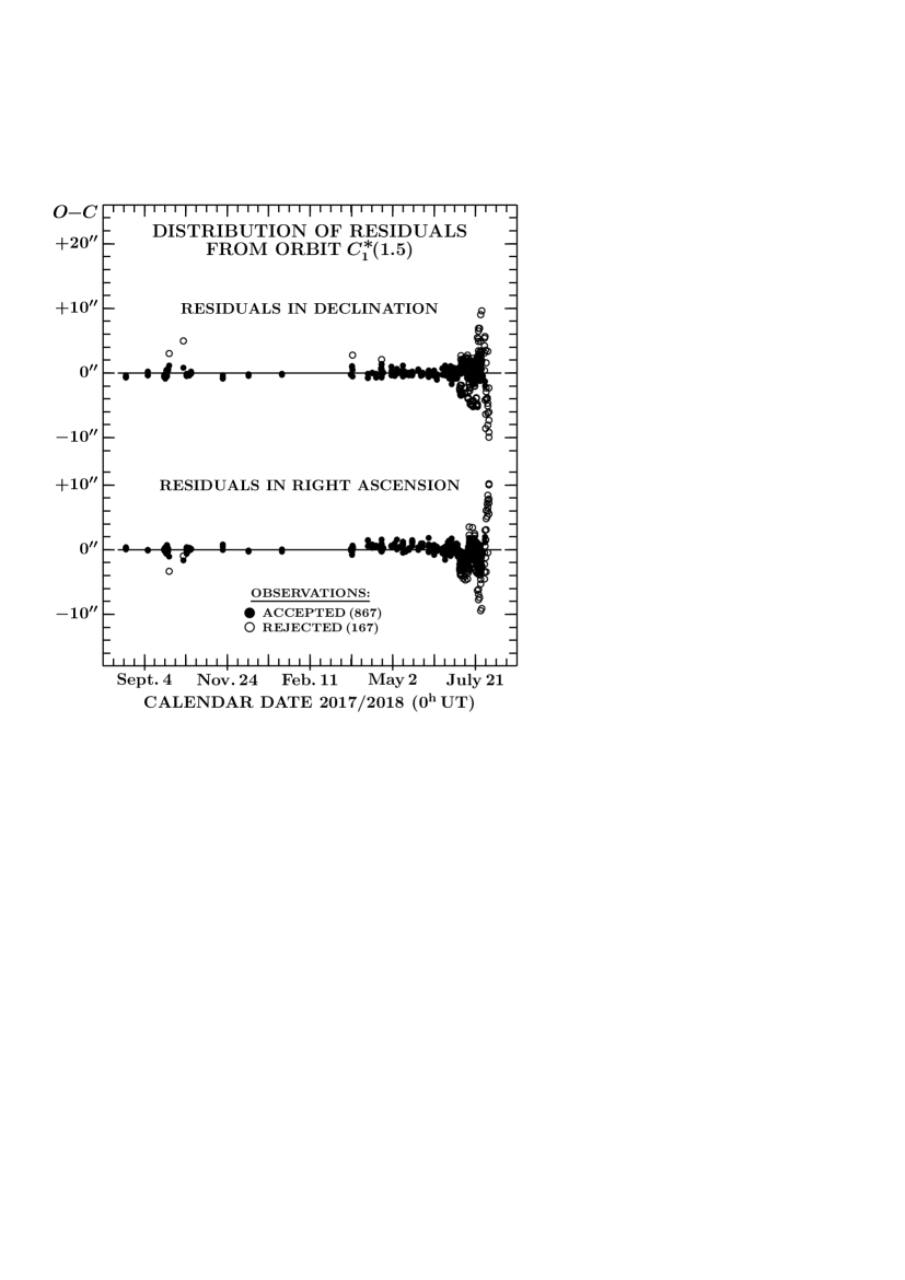
Figure 16.— Distribution of residuals $O\!-\!C$ of 1034 ground-based observations from Orbit C${}_{1}^{\textstyle\ast}$(1.5) (rejection cutoff at 2${}^{\prime\prime\!}$.0). Note the marginal systematic trends in right ascension peaking in April and the overall range of the rejected residuals after Outburst II, in July–August, reaching $\sim$20^′′ in either coordinate.

Although we could have continued to explore modified solutions with still lower scaling distances, we stopped at $r_{0}=1.3$ AU because of an increase to 17^′′ in the magnitude of the residuals, in both coordinates, of rejected observations from early August 2018, even though the systematic trend in the residuals in right ascension, peaking in April 2018, vanished completely. A gradual removal of this trend with decreasing scaling distance is clearly seen from comparsion of Orbit C${}_{1}^{\textstyle\ast}$(2.0) in Figure 15 with Orbit C${}_{1}^{\textstyle\ast}$(1.5) in Figure 16. Other solutions between Orbits C${}_{1}^{\textstyle\ast}$(2.0) and C${}_{1}^{\textstyle\ast}$(1.3) have intermediate properties. The orbits with the scaling distance of 1.3–1.5 AU also offer the best approximations to the original semimajor axis (Table 9) and leave the smallest systematic deviations from the STEREO-A positional data. On balance, we slightly prefer Orbit C${}_{1}^{\textstyle\ast}$(1.5) to C${}_{1}^{\textstyle\ast}$(1.3), because the former leaves the residuals of rejected observations in early August substantially lower, not exceeding $\sim$10^′′; the elements are presented in Table 10.

For comparsion we also computed the distribution of residuals from the MPC orbit by Williams (2018) (reproduced in Table 3); it is displayed in Figure 17. Even though the MPC solution has one more free parameter than the modified-law solutions in Table 9, the systematic trend in the residuals in right ascension that peak in April 2018 is much more prominent, having an amplitude of 3^′′. In addition, the MPC orbit accommodates some 50 fewer observations (at the same rejection level of 2${}^{\prime\prime\!}$.0) than the modified-law solutions with $r_{0}\leq 1.5$ AU and its mean residual is substantially higher. The MPC orbit also leaves asymmetric, systematic trends of up to 12^′′ in the residuals from the rejected July–August ground-based observations and, just as the modified-law solutions, it fails to fit the STEREO-A astrometric observations from Table 4. The poor fit may also have led to the strongly elliptical original orbit, which is evidently inconsistent with both our and Nakano’s results.

Figure 17.— Distribution of residuals of 1034 ground-based observations from the MPC orbit by Williams (2018), based on the standard nongravitational law and 823 data points that satisfy a rejection cutoff at 2${}^{\prime\prime\!}$.0. The solution includes the parameters of the radial and transverse components of the nongravitational acceleration. Note that the systematic trend in the residuals in right ascension stretching from November 2017 through May 2018 is quite formidable, amounting to at least 3^′′ in April. Besides, the residuals of the rejected ground-based observations in late July and early August 2018 are asymmetric and extend to $\sim$12^′′ in declination.

While the modified-law orbits with the scaling distance of 1.3–1.5 AU are superior to the standard-law solutions because they are more successful in simulating the apparent absence of nongravitational effects in the comet’s motion before Outburst I (which began at a heliocentric distance of 1.25 AU), we feel that the effort aimed at accommodating the full range of ground-based observations, from 2017 August 17 to 2018 August 3, by a single set of orbital elements is too ambitious given the perceived anomalies in the comet’s motion especially during Outburst II. These nongravitational perturbations were not only substantial in magnitude but also tightly constrained in time. They cannot be fully accounted for by methods that are designed to describe an essentially continuous action of nongravitational forces. In the following, we employ analogy with cometary splitting in our quest to gain a greater insight into the enigmatic orbital behavior of comet C/2017 S3.

8. Nucleus’ Fragmentation: Detection of
Two Independent Clouds of Debris,
and Their Physical Properties

In Section 7.2 we pointed out that the strong systematic trends in the fragmented nucleus’ residuals from the (extrapolated) orbital motion of the intact comet mimicked the motion of a companion fragment, after its separation from the parent comet, relative to the primary fragment — the problem of a split comet. Because the motion of the intact nucleus of C/2017 S3 was unaffected by a nongravitational acceleration, it is imperative that the residuals from a gravitational orbital solution be employed in this exercise.

As with any other motions driven mainly by a differential deceleration (rather than a relative velocity), the separation between the fragments first increases very slowly, because the deceleration needs time to build up the velocity, which in turn needs time to build up the separation distance. However, in the advanced stages of fragment separation the relative motion increases at rates that increase rapidly. The introduction of the deceleration as the dominant factor in this process always results in a much earlier time of fragmentation relative to the time determined by the models that attribute the effect to an (exaggerated) separation velocity. The needed fragmentation-time corrections can in some instances become enormous.

This major fragmentation-time correction and the slow buildup of the separation distance between the fragments implies that they cannot be spatially resolved for a fairly long time after the event took place, and that therefore only the resulting duplicity or multiplicity of a comet is detected by ground-based observers, not the splitting itself, despite frequent claims to the contrary.

Application of the model by Sekanina (1977, 1982) requires that the fragmentation time of the cloud of nuclear debris of C/2017 S3 be equated with the companion’s time of separation and the effect of solar radiation pressure on the debris particulates with the companion’s nongravitational acceleration, which the model assumes to vary as the inverse square of heliocentric distance. The degree to which the additional condition of an isotropic expansion of the cloud of dust debris (Section 7.2) is in fact satisfied should be tested by checking the absence of a separation-velocity effect.

Equipped with the outlined methodology, our primary interest was to apply the fragmentation model to the rapidly increasing residuals from Orbit B₀ days after the onset of Outburst II, as depicted in Figure 11. A less prominent effect of the same kind appears to be displayed by the distribution of residuals from Orbit A₀ left by the observations made between Outburst I and Outburst II, as shown in Figure 9. For analysis of the process of fragmentation related to Outburst II, we chose Orbit B₀ as the most appropriate reference, in part because it absorbs much of the modest nongravitational perturbation effect associated with Outburst I.

Figure 18.— Evidence of sudden fragmentation of the comet’s nucleus associated with the two outbursts, I and II. The thick curves fit the offsets, from Orbit B₀, of the observations used in the specified solution (solid circles); the thin curves show the other fit (left vs right); and the crosses are the ignored observations. Rejection threshold at 2${}^{\prime\prime\!}$.0. Left: Fit to 367 observations made between July 16 and 31, indicating a fragmentation time of July 15.9 $\pm$ 0.1 UT (1.5 days after the onset of Outburst II) and a nongravitational deceleration of 216 $\pm$ 6 units of 10^-5 the Sun’s gravitational acceleration or (64 $\pm$ 2)$\,\times 10^{-8}$ AU day^-2. None of the 12 data points obtained on August 1–3 and only one out of 23 (or 4 percent) obtained from July 30 on could be accommodated, the remaining ones deviating from the least-squares solutions by more than 2^′′ in at least one coordinate. Right: Fit to 86 observations made between July 23 and August 3, indicating a fragmentation time of July 1.5 $\pm$ 0.7 UT (1.3 days after the onset of Outburst I) and a nongravitational deceleration of 57 $\pm$ 2 units of 10^-5 the Sun’s gravitational acceleration or (16.9 $\pm$ 0.6)$\,\times 10^{-8}$ AU day^-2. We were able to accommodate 9 out of 12 data points obtained on August 1–3 and 13 out of a total of 23 obtained from July 30 on, that is, 75 and 58 percent, respectively.

8.1. Effect of Outburst II in Ground-Based Observations

Treated as offsets from Orbit B₀, the residuals from Figure 11 are replotted, from July 16 on, in the left-hand side panel, and from July 1 on in the right-hand side panel, of Figure 18. We first focus on the left-hand side panel of the figure and notice that, consistent with expectation, in the early days after the onset of Outburst II the offsets are distributed along the axis of abscisas, very slowly building up a detectable deviation from it. Later on, the offsets grow at a sharply accelerating rate, both in right ascension and declination. It is noted that a least-squares fit to the offsets in this advanced stage only would show that the fragmentation occurred some time on July 20 or 21. As long as the scientist is not concerned with the physical implications of the orbital solution, he would incorporate the observations from up to July 20 or 21 into his input file — just as did Nakano (2018b). However, fitting the offsets with the fragmentation model shows that the breakup did indeed take place nearly a week earlier. Applying the model to 367 offsets between July 16 and 31 and choosing a rejection cutoff of 2${}^{\prime\prime\!}$.0, we obtain a solution with a mean residual of $\pm$0${}^{\prime\prime\!}$.77, resulting in a fragmentation time of July 15.9 $\pm$ 0.1 UT, which is lagging the onset of Outburst II by 1.5 days and coinciding with the event’s brightness peak (Figure 1). The deceleration $\gamma$, implied by the rapidly increasing offsets, amounts to 216 $\pm$ 6 units of 10^-5 the Sun’s gravitational acceleration and is equivalent to (64 $\pm\,2)\!\times\!10^{-8}$AU day^-2 at 1 AU from the Sun. At an assumed bulk density of 0.53 g cm^-3, the dominant dust grains in the debris cloud were, following Equation (17), exactly 1 mm in diameter.

This deceleration is nearly identical in magnitude to the value reported by Sekanina & Chodas (2012) for the sungrazing comet C/2011 W3 (Lovejoy). From their examination of its spine tail, they determined for the debris, released from the disintegrating comet shortly after perihelion, a radiation-pressure effect of $\gamma=191$ $\pm$ 42 units of 10^-5 the Sun’s gravitational acceleration. Among the split comets, the short-lived companion to C/1942 X1 (Whipple-Fedtke-Tevzadze), observed over a period of only nine days by G. Van Biesbroeck, was subjected to a similar deceleration, equaling 228 $\pm$ 16 units of 10^-5 the Sun’s gravitational acceleration (Sekanina 1979, 1982).

We also ran solutions that included, as additional parameters, the normal and/or transverse components of the separation velocity only to find that they both were insignificant, with no effect on the result. Accordingly, we see no reason for questioning the validity of the two-parameter solution.

A caveat of major consequence does, however, pertain to the discarded observations. Employing a rejection threshold of 2^′′, we found two groups of offsets in right ascension and/or declination that could not be used because of their unacceptably large deviations from otherwise a very satisfactory fit. The first group was about two dozen offsets on July 16–26, an overwhelming majority of which had the same observatory code, undoubtedly an observer/instrumental problem. The other group was also about two dozen offsets, from July 29–August 3, at the very end of the orbital arc observed from the ground. All these rejected data are depicted by the crosses in the left-hand side panel of Figure 18. Only one offset satisfied the solution on July 29, another one on July 31, but not a single one on August 1–3; over 90 percent were systematically off. In the context of this discrepancy, we recall reports by independent observers (Section 3) that in late July and early August the comet essentially lost its nuclear condensation, aggravating positional determination. But Soulier, who contributed more than 25 percent of the astrometric data reported for July 27–August 3 and 50 percent of the data reported for August 1–3, not only complained that it was difficult to measure the comet’s position (by applying a centroid routine of the Astrometrica software tool), but also pointed out that the comet did not occupy the expected position, as if it were completely displaced.

8.2. Effect of Outburst I in Ground-Based Observations

The remarkable, albeit entirely unexpected, property of the rejected offsets from July 29–August 3 on the left of Figure 18 is their well-organized distribution with time, which is obvious to the extent that we could not resist subjecting these data to the same kind of treatment as the offsets with a confirmed reference to Outburst II. We initiated the procedure by collecting all 23 data reported for July 30–August 3 and by applying the two-parameter fragmentation model. The result of this first step was most surprising: we obtained July 1.9 $\pm$ 5.9 UT for the fragmentation time, a value that is centered on the time lagging the onset of Outburst I by 1.7 days; and a deceleration $\gamma=61$ $\pm$ 15 units of 10^-5 the Sun’s gravitational acceleration. The mean residual was $\pm$3${}^{\prime\prime\!}$.2, the maximum residual amounting to 8^′′. This solution provides us with clear evidence of a surviving cloud of debris related to Outburst I, a feature similar to the cloud associated with Outburst II, but whose existence we have as yet been unaware of.

The large errors are caused by a long gap between the fragmentation time and the short period of time occupied by the offsets, as well as by our refraining from applying any rejection cutoff in this particular case. Next we searched for all offsets between July 23 and August 3 consistent with the initial solution. Re-imposing the 2^′′ rejection threshold, we collected 86 offsets and solved for the two parameters again. We obtained a fragmentation time of July 1.5 $\pm$ 0.7 UT, centered on 1.3 days after the onset of Outburst I. The deceleration was 57 $\pm$ 2 units of 10^-5 the Sun’s gravitational acceleration, equivalent to (16.9 $\pm$ 0.6)$\times 10^{-8}$ AU day^-2 and implying, on the same bulk-density assumption as before, the dominant presence of dust grains 3.8 mm across. The mean residual was $\pm$0${}^{\prime\prime\!}$.98 and the run is depicted in the right-hand side panel of Figure 18.

As with the other debris cloud, we also ran three- and four-parameter solutions that would determine the normal and/or transverse components of the separation velocity, but they always were very near zero. The deceleration resulting from the adopted two-parameter solution, is remarkably close to the value of the $A_{1}$ parameter of the previously derived nongravitational Orbit B${}_{1}^{\textstyle\ast}$(2.0), which was linking the observations covering the orbital arc up to the beginning of Outburst II (Table 8). This encouraging agreement suggests that the debris cloud associated with Outburst I did affect the comet’s astrometry at the time between the outbursts, governing the nongravitational solution.

The residuals from the two-parameter solutions to the debris clouds related to the two outbursts are presented in Table 11 for all ground-based astrometric observations made between July 27 and August 3. In the upper half of the table, covering July 27–29, the observations refer mostly to the debris cloud associated with Outburst II, while its lower half, July 30–August 3, is dominated by the observations of the debris cloud related to Outburst I. The same result emerges from the summary Table 12, which lists daily totals of the observations: their numbers have a tendency to increase with time for the debris cloud associated with Outburst I, but to decrease for the cloud related to Outburst II. The time at which the numbers of the two trends equate each other is not sharply defined, but Table 11 and Table 12 consistently suggest that this happens in general proximity of July 29/30. Since it is the peak surface brightness that determines the spot the measurers bisect as the “comet’s position”, the transition from one cloud to the other suggests that they were then of approximately equal peak surface brightness, one fading more steeply than the other. We show in Section 8.4 that the critical time, $t_{\rm crit}$, when the balance was achieved — adopted to have occurred on July 30.0 UT — provides an important piece of information, despite the fact that the fading trends are at first sight counterintuitive.

8.3. Split-Comet Scenario

The comet’s nuclear condensation, determining the comet’s astrometric position, was measured with high accuracy as a well-behaving peak of light until the time of Outburst I. This is documented by a low mean residual of $\pm$0${}^{\prime\prime\!}$.45 of Orbit A₀ and a very few observations that had to be discarded because their residuals exceeded the rejection threshold of 1${}^{\prime\prime\!}$.5 (see Appendix).

Starting with Outburst I, C/2017 S3 became effectively a double comet. During this event, the major part of the parent nucleus became the primary fragment, while the less sizable part began disintegrating, presumably upon separation, into a compact cloud of debris. The active phase of the event was characterized by a sharp, starlike condensation — typical for comets in outburst — consisting primarily of the emitted gas and microscopic dust ejecta, the latter being confirmed by an instant increase in the Af$\rho$ parameter (e.g., Bryssinck, footnote 1). The parallel surge of total brightness was dominated by gas, as already acknowledged in Sections 1 and 4.2. The contribution by the cloud of millimeter-sized debris remained largely obscured for a number of days, until the activity of the primary fragment subsided enough. Only then did the chances of the cloud’s detection improved, especially in properly centered small apertures used in astrometric observations, with the opportunity peaking just before the onset of Outburst II.

With the arrival of Outburst II, all traces of the previous activity got concealed by the newly developing feature. Within two days of the event’s onset, the primary fragment appears to have completely disintegrated into a second cloud of debris, believed to be much more massive but also rapidly expanding with time. Measured astrometric positions, referring to the bright and initially stellar nuclear condensation at the location of the disintegrating nucleus, did not begin to deviate from the extrapolated Orbit B₀ until July 20/21, suggesting that, by then, the cloud of millimeter-sized grains associated with Outburst II began to dominate the comet’s brightness in the small apertures. The expansion rate of this cloud, given by Equation (15), explains the sharp drop in the nuclear-condensation’s brightness seen in Figure 1. If the cloud of millimeter-sized grains related to Outburst I was expanding, as it turned out to be the case, at a much lower rate, the surface-brightness peak at this cloud’s center was dimming with time more slowly than the peak of the debris cloud associated with Outburst II; it was only a matter of time for the former outshining the latter. As documented by their astrometry, this is exactly what Soulier and other observers detected in the period of July 30 through August 3: the bisected point of maximum surface brightness moved from the debris cloud related to Outburst II to that related to Outburst I; the comet looked displaced, as illustrated in Figure 18.

The existence of two nearby peaks in the coma at the time is corroborated by Soulier’s (see footnote 15) brightness measurements in two apertures on August 3.12 UT. Magnitude 16.2 in a 6${}^{\prime\prime\!}$.5 peak-centered aperture implies a magnitude fainter than 12.7 in a 32${}^{\prime\prime\!}$.4 aperture, yet Soulier reports magnitude 11.5. Since there was no major condensation in the coma, the discrepancy implies that the second peak was likely to have been located within the larger aperture’s radius; Table 11 does indeed predict that the two clouds’ centers were then about 22^′′ apart.

Figure 19.— Projected trajectories of the clouds of millimeter-sized dust grains relative to the extrapolated Orbit B₀. Although the breakup occurred on July 1.5 UT for the cloud related to Outburst I and on July 15.9 UT for the cloud related to Outburst II, either cloud remained close to the position determined by Orbit B₀ for an extended period of time following the fragmentation event. For example, the separation distance of 2^′′ was reached only two weeks after fragmentation in the first case and 5 days after fragmentation in the second case. There was no need to introduce a separation velocity in order to fit the motions of the two debris clouds, either one of which moved under the effects of a repulsive force that varied as an inverse square of heliocentric distance and is believed to be solar radiation pressure. The deceleration on the cloud related to Outburst II was 3.8 times higher than on the other cloud.

In summary, the distribution of offsets of the observed positions from Orbit B₀ conforms closely to a concatenated curve representing the motions of two distinct clouds of millimeter-sized dust grains that were released during the two major outbursts, always some 1–2 days after their onset. The debris cloud associated with Outburst I fits (i) the offsets at times between the outbursts (although these offsets were not used in the solution, they stayed within 2^′′ and the cloud’s motion essentially coincided with the center of the nuclear condensation that appeared after Outburst I): (ii) some of the offsets between July 23 and 27; and, most importantly, (iii) nearly all offsets from July 30 on; but not between July 16 and 22. The cloud of millimeter-sized grains related to Outburst II fits the offsets in the period of time between July 16 and 27, but only sporadically those at the later time, and none on August 1–3. Between July 23 and 28 the projected motions of the two clouds were close enough to each other that it is difficult to resolve to which any particular observation referred. The centers of the two clouds had equal right ascension on July 25.5 UT and equal declination on July 27.0 UT. The separation distance between them increased to 13^′′ on August 1 and to about 22^′′ on August 3. Although the disintegrating object was technically a double comet, this status was concealed by the described configuration and brightness relationship between the two components The trajectories of the two debris clouds relative to the extrapolated Orbit B₀ are plotted in Figure 19.

8.4. Condition of Equal Peak Surface Brightness, and Properties of Debris Cloud Related to Outburst I

The condition of equal peak surface brightness implies constraints on the relationship between the expansion velocities, $v_{\rm exp}$, and the total projected scattering cross-sectional areas, $X_{\rm frg}$, of the two debris clouds. A cloud’s surface brightness is proportional to the sum of the cross-sectional areas of the grains situated in a column of unit projected area that extends along the line of sight. In an isotropic and uniformly expanding, optically thin spherical cloud of debris (see Section 5), which at time $t$ projects as a disk of radius $\rho(t)$, the surface brightness decreases symmetrically with increasing distance $x$ from the center of the disk. The sum of the cross-sectional areas of the grains located inside a column of unit projected area at distance $x$ from the disk’s center equals $\sigma(t,x)$ and varies as the column’s length,

$$\sigma(t,x)\sim\sqrt{\rho^{2}\!-\!x^{2}}.$$ (19)

The surface brightness reaches a peak at the center of the disk, where $\sigma(t,0)\equiv\sigma_{0}(t)$, so that

$$\sigma(t,x)=\sigma_{0}(t)\sqrt{1\!-\!\left(\frac{x}{\rho}\right)^{\!\!2}}.$$ (20)

A total cross-sectional area of all grains in the cloud is calculated by integrating over the disk,

$$X_{\rm frg}=\!\!\int_{0}^{\rho}\!\!2\pi x\sigma(t,x)\,dx={\textstyle\frac{2}{3}}\pi\sigma_{0}\rho^{2}.$$ (21)

While $\sigma_{0}$ and $\rho$ vary with time, $X_{\rm frg}$ is for either cloud a constant, so $\sigma_{0}\!\sim\!\rho^{-2}$. Inserting for $\rho$ from Equation (1); referring, respectively, to the fragmentation time, the expansion velocity, the peak columnar cross-sectional area of the grains (determining the peak surface brightness), and the total cross-sectional area of the cloud of debris associated with Outburst I as $t_{\rm frg}$(I), $v_{\rm exp}$(I), $\sigma_{0}$(I), and $X_{\rm frg}$(I); referring, respectively, to those associated with Outburst II as $t_{\rm frg}$(II), $v_{\rm frg}$(II), $\sigma_{0}$(II), and $X_{\rm frg}$(II); and equating, at time $t_{\rm crit}$, the two peak values of the surface brightness (i.e., the sums of the peak cross-sectional areas of the grains); we find for the relationship between the two events’ parameters:

$$\frac{X_{\rm frg}{\mbox{({\scriptsize I})}}}{v_{\rm exp}^{2}{\mbox{({\scriptsize I})}}\left[t_{\rm crit}\!-\!t_{\rm frg}{\mbox{({\scriptsize I})}}\right]^{2}}=\frac{X_{\rm frg}{\mbox{({\scriptsize II})}}}{v_{\rm exp}^{2}{\mbox{({\scriptsize II})}}\left[t_{\rm crit}\!-\!t_{\rm frg}{\mbox{({\scriptsize II})}}\right]^{2}}.$$ (22)

In this dimensionless equation we know $t_{\rm frg}$(I) and $t_{\rm frg}$(II) from, respectively, Sections 8.2 and 8.1; $v_{\rm exp}$(II) from Equation (15); $X_{\rm frg}$(II) from Equation (12); and $t_{\rm crit}$ from Section 8.2. Equation (22) can be written as a relation between the two unknowns,

$$X_{\rm frg}{\mbox{({\scriptsize I})}}=\eta\,v_{\rm exp}^{2}{\mbox{({\scriptsize I})}},$$ (23)

where

$$\eta=\frac{X_{\rm frg}{\mbox{({\scriptsize II})}}}{v_{\rm exp}^{2}{\mbox{({\scriptsize II})}}}\left[\frac{t_{\rm crit}\!-\!t_{\rm frg}{\mbox{({\scriptsize I})}}}{t_{\rm crit}\!-\!t_{\rm frg}{\mbox{({\scriptsize II})}}}\right]^{\!2}\!\!.$$ (24)

Numerically, $\eta=1.56\times\!10^{6}$ s².

In Section 8.3 we suggested that the contamination of the cloud of millimeter-sized grains associated with Outburst I should have been minimized shortly before the onset of Outburst II, although the question of what fraction of the comet’s brightness it accounted for remains open. An example for testing the cloud’s signal is the observation on July 14.03 UT by E. Bryssinck (see footnote 1), who reported the apparent red magnitude of 14.24 in an aperture 9${}^{\prime\prime\!}$.92 in radius and of 15.56 in an aperture 4${}^{\prime\prime\!}$.96 in radius. They are equivalent to the phase-corrected absolute magnitudes of 13.37 and 14.69, respectively. To find out whether at this time $t_{\rm obs}$ the debris cloud, of an expansion-velocity dependent radius $\rho_{\rm obs}$ extended beyond the limits of an aperture of radius $a_{\rm obs}$, we checked the validity of Equation (6). Denoting the cross-sectional area of the debris cloud inside the aperture at the time of observation as $X_{\rm obs}$, the equation can be rearranged thus:

$$\left[1\!-\!\frac{\xi}{v_{\rm exp}^{2}{\mbox{({\scriptsize I})}}}\right]^{\!2}\!\!=\!\left[1\!-\!\frac{\zeta}{v_{\rm exp}^{2}{\mbox{({\scriptsize I})}}}\right]^{\!3}\;\;\;\;({\rm for}\;\rho_{\rm obs}\!>\!a_{\rm obs}),$$ (25)

where with use of Equation (23),

$$\xi=\frac{X_{\rm obs}}{\eta},\;\;\;\;\zeta=\!\left[\frac{a_{\rm obs}}{t_{\rm obs}\!-\!t_{\rm frg}{\mbox{({\scriptsize I})}}}\right]^{\!2}\!\!,$$ (26)

and $X_{\rm obs}$ is expressed as a function of the absolute magnitude according to Equation (11). If the flux of the cloud of millimeter-sized grains associated with Outburst I is contaminated in the aperture by other ejecta, one gets an upper limit on $X_{\rm obs}$.

The condition (25) is a quadratic equation in $v_{\rm exp}^{2}(\mbox{\scriptsize I})$, with meaningful solutions limited to

$$\zeta<\xi<{\textstyle\frac{3}{2}}\,\zeta$$ (27)

and to the root with the positive sign in front of the discriminator. Writing further $\xi=\zeta(1\!+\!\epsilon)$ (with $0\!<\!\epsilon\!<\!\frac{1}{2}$), the solution becomes

$$v_{\rm exp}^{2}(\mbox{\scriptsize I})=\zeta\!\left[1\!-\!\epsilon\!\left(\!1\!+\!{\textstyle\frac{1}{2}}\epsilon\!+\!\sqrt{\epsilon}\sqrt{1\!+\!{\textstyle\frac{1}{4}}\epsilon}\right)\!\right]^{\!-1}\!\!.$$ (28)

Returning now to the July 14 observation by Bryssinck, the results for the larger aperture, 9${}^{\prime\prime\!}$.92 in radius, are $\xi=58.5$ m² s^-2 and $\zeta=66.8$ m² s^-2, so that the condition (27) is not satisfied. The dimensions of the cloud related to Outburst I are smaller than the aperture, and its expansion velocity is lower than $\sqrt{\xi}=7.6$ m s^-1, which happens to be a tenth of the expansion velocity of the cloud associated with Outburst II. This result already suggests that Outburst I was a far less violent event than Outburst II.

For the smaller aperture, 4${}^{\prime\prime\!}$.96 in radius, the condition (27) is satisfied, even though only marginally. We derive $\xi=17.3$ m² s^-2 and $\zeta=16.7$ m² s^-2, so that $\epsilon=0.0359$ and the solution (28) then implies an expansion velocity of $v_{\rm exp}({\mbox{\scriptsize I}})=4.18\;{\rm m}\;{\rm s}^{-1}$, unless the observed signal’s contamination by other ejecta (e.g., microscopic dust) exceeds 3–4 percent. On the same assumption we have for the cross-sectional area of the cloud from Equation (23) $X_{\rm frg}({\mbox{\scriptsize I}})=27\;{\rm km}^{2}$, only a little more than 1 percent of the cross-sectional area of the cloud related to Outburst II.

In order to test the validity of the assumption on the lack of a major contamination of the measured signal, we confront the result based on the July 14 observation with the last ground-based observations, made by Soulier on August 3.11–3.12 UT, when he used an aperture of 6${}^{\prime\prime\!}$.5 in radius to measure an average apparent CCD magnitude of 16.4 (see footnotes 5 and 15). Comparison of Soulier’s unfiltered CCD magnitudes and Bryssinck’s red magnitudes suggests that after aperture correction they are essentially equal, so we apply no color correction. Soulier’s phase-corrected absolute magnitude on August 3 is then 18.6, constraining the projected area of the cloud to

$$X_{\rm frg}({\mbox{\scriptsize I}})<0.8\;{\rm km}^{2}$$ (29)

and for the expansion velocity

$$v_{\rm exp}({\mbox{\scriptsize I}})<0.7\;{\rm m}\>{\rm s}^{-1}\!.$$ (30)

This indicates that the cloud of millimeter-sized grains associated with Outburst I was detected only in the images taken on the final days of the comet’s ground-based monitoring campaign; that in the examined July 14 image the cloud contributed no more than a few percent of the signal in the smaller aperture; that the expansion velocity was in a range that is typical for the separation velocities of the split comets; and that Outburst I should be classified as a nonfatal event.

8.5. Results from the STEREO-A Images

Because of the 72^′′ pixel size of the HI1 imager’s detector, one should not read too much into the information provided by the STEREO-A astrometric positions listed in Table 4. The very fact that they refer to the debris cloud associated with Outburst II comes from their photometry (Section 5), not astrometry.

The fragmentation solution derived from the ground-based observations in Section 8.1 (a fragmentation time of July 15.9 UT and a radial nongravitational acceleration of 64$\,\times 10^{-8}$ AU day^-2 at 1 AU from the Sun based on an inverse square power law of heliocentric distance) fits the 46 STEREO-A positions, including the several clearly inferior points, with a mean residual of $\pm$29${}^{\prime\prime\!}$.1. The few final positions, which left huge negative residuals in right ascension, of up to $\sim$170^′′ from Orbit A₀ (Figure 10) and up to $\sim$100^′′ from Orbit B${}_{1}^{\textstyle\ast}$(2.0) (Figure 14), are now accommodated with residuals of $<$30^′′.

No fragmentation time can at all be determined from the STEREO-A data set alone and no meaningful results are obtained by differentially correcting more than three fragmentation model’s parameters at a time. When the fragmentation time is fixed at July 15.9 UT, various solutions with a mean residual of less than $\pm$15^′′, or one fifth of the pixel size, are derived, their only common attribute being a nongravitational-acceleration parameter $A_{1}$ that exceeds the value obtained from the ground-based observations. The parameter’s value is now close to 100 $\times 10^{-8}$ AU day^-2 (instead of 64 $\times 10^{-8}$ AU day^-2), which by itself suggests that by the time the cloud of debris left the field of view of the STEREO-A imager shortly before perihelion, the dominant diameter of dust grains in the cloud dropped to $\sim$0.7 mm or less, possibly a sign of their incipient sublimation. Because of the fashion in which orbital data respond to sudden events (Section 7.2), this effect could reflect the precipitous dive of the debris cloud’s intrinsic brightness detected in the last several STEREO-A images (Figure 3).

8.6. Unconfirmed Post-Perihelion Ground-Based
Observations of the Comet’s Debris

J. J. González reported his visual detection of the comet’s debris with his 20-cm f/10 Schmidt-Cassegrain telescope on five nights between 2018 October 16 and November 16, estimating the total magnitude of the essentially condensation-free cloud consistently at 9.7–10.1. The feature’s diameter was near 4^′ in October (when located low above the horizon), but 8^′–9^′ in November (when it was higher). On the last date, this cloud, observed at magnification of 77$\times$, was surrounded by a “wide and very diffused extension” to 1${}^{\circ}\!$.2, of complex morphology and elongated along the orbit.

On November 20, A. Hale inspected the region of the predicted position of the comet with his 41-cm f/4 reflector, detecting no trace of it with certainty. On November 20.504 UT, M. Suzuki imaged a field of 49^′ by 32^′ centered on the ephemeris position with a 43-cm f/4.5 telescope (+CCD) of the Remote Astronomical Society Observatory of New Mexico near Mayhill. Visual inspection of the 6-minute exposure reveals no sign of any comet-related mass. The question we address below is whether it is possible to reconcile González’s detection with Suzuki’s and Hale’s negative observations. At issue is the contrast threshold (or sensitivity) of a visual observer and a CCD device.

The most comprehensive investigation of the contrast threshold of human vision was performed by Blackwell (1946), who employed 19 highly trained observers with visual acuity of 20/20, each contributing tens of thousands of individual data to the published sample. More recent reviews and studies of the subject (e.g., Clark 1990; Crumey 2014; Montrucchio 2015) still build on Blackwell’s results.

Blackwell examined the contrast threshold as a function of two fundamental parameters, both highly relevant to our topic. One was the luminance of a uniform background and the other was the angular size of the target disk (stimulus). In the experiments he considered both positive contrasts (targets brighter than the background) and negative. The brightness of the night sky is well within the range he studied (the work was motivated in part by the night-operations needs of the U.S. military that funded it), but the largest stimulus was merely 6^∘ in diameter. Fortunately, for extended targets the contrast threshold varied little and predictably with size, allowing sound extrapolation. Blackwell did not examine the dependence of the contrast threshold on other possible variables, including the observer’s age that Montrucchio (and others) found to be important.

González made the reported observations at two high-elevation locations and provided much relevant information needed for judging the accuracy of his reports, including the site’s Sky Quality Meter’s (SQM) measurement. In all five instances the luminance of the feature, computed from its estimated total brightness and diameter, was above the expected average contrast threshold, by a factor of 10 or more in October and by about 2 in November, when the feature’s surface brightness was, on the average, 67 $\pm$ 11 S₁₀ units, equaling 9 $\pm$ 2 percent of the background sky brightness. A suspicious attribute of the reported feature is the sharp drop in its surface brightness by a factor of $\sim$6 between October and November.

The dependence of the contrast sensitivity on a wide range of conditions under which a visual observation is made does not rule out the possibility that Hale’s threshold was close to, or exceeded, the feature’s inferred surface brightness, in line with his failure to detect it. Of greater concern is the feature’s apparent absence in the image taken by Suzuki.

Unlike González’s observations, the CCD image is accompanied by few details. This observation was made shortly before the beginning of the astronomical twilight, with the comet at a zenith distance of 58^∘ and the Sun 19${}^{\circ\!}$.5 below the horizon at midexposure. The Moon was also below the horizon, and the high altitude of the observatory (higher than González’s observing sites) should have provided near-perfect conditions. We do not know the contrast threshold of the CCD device used, but it certainly was substantially better than visually (probably $<$ 1 S₁₀). We would only question whether visual inspection of the image is enough to claim that the feature does not show up in it. We are unaware of any more rigorous means of examination or an image-enhancement technique having been applied. It is perhaps likely, but not certain, that we have a problem.

In support of the possible conflict, we should point out that the total magnitudes reported by González imply a phase-corrected absolute magnitude as bright as 6.7 in October and 6.1 in November 2018. These do not reconcile easily with the absolute magnitudes of 10.7 for the intact comet before Outburst I (Section 4.2) and 9.9 for the debris cloud after Outburst II (Section 5), not to mention the sudden drop noted in the last STEREO-A images shortly before perihelion, when the absolute magnitude slumped to 11.3 and the brightness was subsiding at a rate of 0.8 mag per day (Table 1). The only physically plausible mechanism that we know of which could bring about a major intrinsic brightening of a defunct comet after a period of a few months is the process of continuing progressive dust-grain fragmentation. If the mass of millimeter-sized grains at the end of July should have increased its intrinsic brightness more than thirtyfold, their dominant dimension should over this period of time drop by the same factor, i.e., from 1 mm to 30 $\mu$m across. If so, however, they would occupy a strongly elongated volume of space several degrees — not 9^′ — long in a position angle of 210^∘.

The light curve based on the González magnitudes in October–November is also problematic. A plot, against heliocentric distance $r$, of the five magnitude estimates corrected for the geocentric distance and phase effect is flat between 1.5 and 2.1 AU: in the standard law $r^{-n}$ the exponent is calculated to equal $n=0.2\pm 0.3$ instead of the expected $n=2$.

Any other avenue of explaining the González feature would have to be purely speculative. For example, one can postulate that most of the mass of the original nucleus was inert, not participating in activity and not fragmenting, until after the comet left both the fields of view of the HI1 imager on board STEREO-A and the C3 coronagraph on board SOHO, since there is no sign of detection of such an object by either detector. Very impressive observational evidence would be required to make this hypothesis look credible.

We believe that while the existence of a residual mass of the disintegrated comet C/2017 S3 is unquestionable, it is difficult to identify it with the unconfirmed, very bright feature reported by González on five occasions in October–November. It is unfortunate that no additional CCD imaging has been attempted to help resolve this issue.

9. Summary of Properties of the Debris Clouds

Now that we know the total projected areas of the two debris clouds, $X_{\rm frg}$, and the dominant diameter, $D$, of the grains that make them up, we can readily estimate the clouds’ masses at an assumed bulk density $\delta$. Eliminating the number of grains from the expressions for the total projected area and total mass ${\cal M}_{\rm frg}$, we have

$${\cal M}_{\rm frg}={\textstyle\frac{2}{3}}\delta D_{\rm frg}X_{\rm frg}.$$ (31)

Adopting again a bulk density of $\delta=0.53$ g cm^-3 and inserting for Outburst II, $D_{\rm frg}({\mbox{\scriptsize II}})=1$ mm from Section 8.1 and $X_{\rm frg}({\mbox{\scriptsize II}})=2200$ km² from Equation (12), we obtain for the mass of the cloud associated with this outburst

$${\cal M}_{\rm frg}({\mbox{\scriptsize II}})=7.8\times\!10^{11}\,{\rm g},$$ (32)

which equals the mass of a spherical object 140 meters in diameter. Taking for Outburst I, $D_{\rm frg}({\mbox{\scriptsize I}})=3.8$ mm from Section 8.2 and $X_{\rm frg}({\mbox{\scriptsize I}})<0.8$ km² from the relation (29), we similarly find for the mass of this cloud

$${\cal M}_{\rm frg}({\mbox{\scriptsize I}})<1.1\times\!10^{9}\,{\rm g},$$ (33)

equivalent to the mass of a sphere less than 16 meters in diameter. It would add negligibly to the dimensions of an object 140 meters across.

Since the square of a mean outward velocity of the grains that make up a cloud expanding with a velocity $v_{\rm exp}$ equals $\langle v^{2}\rangle=\frac{1}{3}v_{\rm exp}^{2}$, the kinetic energy needed to release the cloud of millimeter-sized grains in the course of Outburst II amounts to

$${\cal E}_{\rm kin}({\mbox{\scriptsize II}})=7.5\times\!10^{18}\,{\rm erg},$$ (34)

while for the cloud conceived during Outburst I the kinetic energy is constrained by

$${\cal E}_{\rm kin}({\mbox{\scriptsize I}})<0.9\times\!10^{12}\,{\rm erg}.$$ (35)

Although an investigation of the physical processes that caused the outbursts is not an objective of this paper, we note that the kinetic energy of the Outburst II cloud amounts to the energy released in the course of the transformation of less than 10¹⁰ g of amorphous water ice into cubic ice at a temperature of $\sim$140 K, given that the relevant heat of crystallization equals 10⁹ erg g^-1 (Ghormley 1968). At a distance of 70 meters from the center of the nucleus, this mass of ice would be contained in a layer of less than 30 cm thick.

The mass and size of the original nucleus of the comet were of course greater than the estimates of the large-debris clouds suggest, although probably not by much. The losses of outgassed ices and emitted microscopic dust integrated over one orbital period about the Sun are for a comet with a perihelion distance of 0.2 AU typically equivalent to a layer several meters deep. Given that C/2017 S3 was a dust-poor comet and that its activity had terminated by the time of Outburst II, prior to perihelion and before the comet reached 0.9 AU, the total losses in the dimensions of the nucleus by gas and dust emission should have been almost trivial. The only significant mass contribution could have derived from sizable undetected fragments of inert material, pebbles and boulders, should they have survived Outburst II.

For an Oort Cloud comet of this size and perihelion distance, it is rather unusual to exhibit no nongravitational effects in the orbital motion about the Sun (Marsden et al. 1978). Yet, C/2017 S3 is found to exemplify this peculiarity before Outburst I, as demonstrated convincingly by our first two solutions, Orbits A₀ and A₁. A rapidly rotating nucleus of a low obliquity may represent a scenario that is in line with the comet’s observed motion. The rapid rotation may also have been a driver of the fragmentation events.

Comparison of the class B solutions, which span a time period that includes Outburst I, shows the presence of moderate nongravitational perturbations. This event did not paralyze the nucleus, but may have acted as a precursor event to Outburst II by providing direct access to the nucleus’ interior over a limited area of the surface, thereby facilitating the looming breakup.

These considerations already suggest that the two outbursts differed from each other markedly. The differences are documented in the upper part of Table 13 that summarizes the information gathered from the photometric data. Besides the quantities measured directly from the light curve (the time of onset, rise time, and amplitude), the listed parameters include quantities that better describe the yield of either outburst’s active stage and provide a more accurate comparison of the two events: the flux rise and its average rate (Sekanina 2017). In particular, the average flux-rise rates confirm that Outburst II was a much more explosive event than Outburst I, a finding that certainly is not obvious from comparison of the two events’ amplitudes or Af$\rho$ values.

Information on the debris clouds is summarized in the lower part of Table 13. The existence of the cloud associated with Outburst II was strikingly demonstrated by the divergence of the residuals left by the post-event observations from the early gravitational orbits (A₀ and B₀) linking the pre-outburst astrometric observations. Thanks to the large-aperture measurements of the cloud’s total brightness in the STEREO-A images taken between July 31 and August 14, it was possible to determine the feature’s expansion rate.

By contrast, we were unaware of the large-debris cloud related to Outburst I until we noticed that the ground-based observations from July 30 to August 3 increasingly deviated from the expected positions of the Outburst II cloud. Although the Outburst I cloud was much fainter, its rate of expansion was extremely low (if any; see below), so that its peak surface brightness eventually exceeded that of the Outburst II cloud in the last days of ground-based observation. Only outer regions of the Outburst II cloud, some 100,000 km in radius by this time, were superposed on the compact Outburst I cloud.

For this reason, Soulier’s imaging on August 3 is shown by the relation (29) to provide only an upper limit on the projected area $X_{\rm frg}$(I). The tight expansion-velocity constraint in the relation (30) does not rule out the limit of $v_{\rm exp}=0$, which would imply that the feature related to Outburst I was not in fact a cloud of debris, but a single sizable subfragment. Its estimated brightness and exposure to moderate radiation-pressure effects are only reconciled if the subfragment was a devolatilized, “fluffy” aggregate of loosely-bound dust grains (i.e., of very high porosity), with the dominant grain diameter definitely smaller than the nominal size (3.8 mm across) and more in line with the dominant size of the grains in the Outburst II cloud. Orbit B${}_{1}^{\textstyle\ast}$(2.0), the best B-class solution (Table 7), suggests that the putative aggregate’s motion was consistent with the motion of the measured condensation that consisted of the debris of the original nucleus’ major fragment that was released in the course of Outburst I and might have been still active for a short period of time afterwards. Late July and early August was apparently the only time when the aggregate subfragment, the surviving part of the major Outburst I fragment, was picked up and monitored, when already inert, for several days by four independent observers (Tables 11 and 12). Survival of such a sizable piece of fluffy nuclear debris is fascinating; major ramifications are addressed in Section 10.

Whatever its nature, the modeling of its motion should have been carried out on the residuals of the relevant observations from Orbit A₀. However, we replaced them with the residuals from Orbit B₀ to mitigate effects of extrapolation. This decision seems justified by the above mentioned agreement between the parameter $A_{1}$ from Orbit B${}_{1}^{\textstyle\ast}$(2.0) and the deceleration from the fragmentation model based on Orbit B₀.

Table 13 shows that fragmentation followed the onset of either outburst by about 1.5 days. While this information is burdened by a large error for Outburst I, the computed uncertainty for Outburst II is only a small fraction of a day, the time of fragmentation coinciding in fact with the time of peak brightness (i.e., the end of the event’s active stage). As a process, fragmentation does not occur instantaneously, yet the data on Outburst II suggest that the duration was very short.

From the information available, we classify Outburst I as a nonfatal event and Outburst II as a cataclysmic event. C/2017 S3 has a special place among comets because enough data are available to classify it equally as a disintegrating comet and a split comet. In its capacity as a split comet, the comet displays a very strong correlation between outbursts and nuclear fragmentation — a topic repeatedly addressed in the scientific literature over the past decades. However, C/2017 S3 is an atypical split comet in that it displays no primary nucleus (its position at any time after an outburst approximated by extrapolating the comet’s pre-outburst purely-gravitational motion) and two companions that have never been measured or, indeed, observed, at the same time.

Fitting a debris cloud’s motion with a constant deceleration implies the presence of a dominant grain size, which may be surprising. These grain dimensions, in the millimeter-size range, are typical for the debris detected in cometary dust trails (e.g., Sykes et al. 1990; Reach et al. 2007) and for meteoroids in related meteor outbursts (e.g., Jenniskens 1998). Dust grains of this size are important in that they are large enough not to get rapidly dispersed in space by radiation pressure, yet small enough to have a rather high cross-section-to-mass ratio for fairly efficiently scattering sunlight and abundant to be readily noticed (unlike pebbles and boulders) in CCD images. Interestingly, the post-perihelion disintegration of C/2011 W3 resulted in a cloud of dust grains whose dominant size (Sekanina & Chodas 2012) was very similar to the size we find for the cloud related to Outburst II.

10. Ramifications

Our investigation of C/2017 S3 has ramifications primarily for short-lived companions of the split comets. Based on the assumption that — as a fragment of the original nucleus — a companion is a miniature comet that sublimates and releases dust, its nongravitational deceleration has been interpreted as the product of the outgassing-driven momentum transfer the same mechanism that was invoked by Whipple (1950) for comets in general. With evidence that either “companion” of C/2017 S3 is an expanding cloud of (inert) millimeter-sized dust grains, the nongravitational deceleration is identified with solar radiation pressure. Could it be that most, if not all, short-lived companions of the split comets are expanding clouds of grains? This idea is corroborated by well-known properties of such companion nuclei, which (i) become more diffuse with time; (ii) grow steadily in size; (iii) get progressively elongated; and (iv) disappear on time scales equivalent at 1 AU from the Sun to days, weeks, or, at most, 1–2 months. The property under (iii) would in this context imply grain crumbling, which increases the radiation pressure. The major difference between the outgassing-driven deceleration and radiation pressure — the variation with heliocentric distance — is mitigated by the short lifetime of the companion nuclei and by the fact that they are mostly observed at smaller distances from the Sun, at which the two mechanisms imply nearly identical rates of variation. Thus, the heliocentric-distance law cannot readily be employed as a criterion to discriminate between the two interpretations and the problem remains open. For persistent companions of the split comets the outgassing-driven deceleration appears to be preferable except perhaps shortly before the end of their lifetime.

We conclude with speculation: Is there a lesson to be learned from the physical behavior of C/2017 S3 that is relevant to 1I/’Oumuamua? Both objects had similar perihelion distances, 0.21 AU and 0.25 AU, respectively, and they both arrived from interstellar space, except that from a distance of 10⁵ AU it took the comet 300 times longer than 1I to get to perihelion. From a distance of 50 AU the ratio is still about 3. This means that the comet could have accommodated to the high temperatures more gradually and its interior was, on the average, subjected to lower thermal stresses, yet C/2017 S3 did disintegrate. Should not one expect 1I to do likewise?

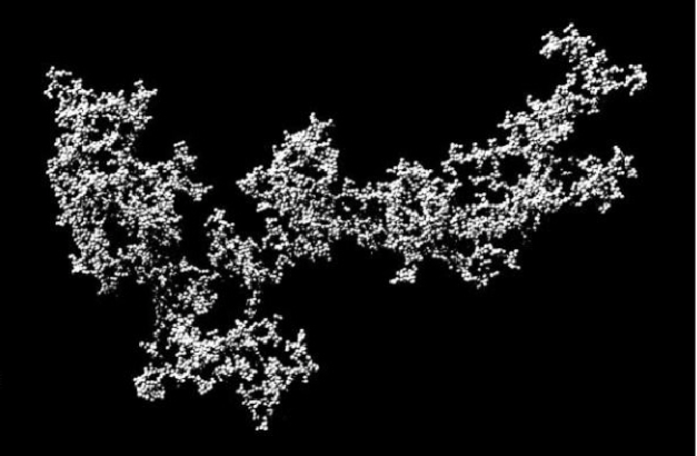
Figure 20.— Computer-generated image of a loosely-bound fluffy aggregate of dust grains (ballistic cluster-cluster agglomeration or BCCA; from Wada et al. 2008), whose effective bulk density may drop below 0.0001 g cm^-3. Models of this kind are devised for studies of formation processes of planetesimals in protoplanetary disks. With the dimensions scaled up, the model is used to simulate outburst-surviving high-porosity fragments of a cometary nucleus. The debris “cloud” associated with Outburst I of C/2017 S3 may have had this kind of morphology, and we propose to apply this paradigm to the interstellar object 1I/‘Oumuamua as well. (Image credit: K. Wada et al., Hokkaido University, Sapporo, Japan.)

A remarkable property of many comets is that their appearance in the same range of heliocentric distances before and after perihelion is very different. For C/2017 S3, the disparity was astounding. Given that the earliest pre-discovery observation of 1I was made five weeks after perihelion, we have absolutely no idea on how the object looked like before perihelion, a great disadvantage compared to C/2017 S3. On the other hand, the post-perihelion near-encounter of 1I with the Earth allowed close-up examination of its physical behavior, which was unavailable for C/2017 S3. In spite of these differences and rather limited supporting evidence, we find it both intriguing and irresistible to suggest that, to a degree, the two objects may have shared a similar recent history in that they both underwent preperihelion outbursts, albeit on different scales, with 1I exhibiting features that were unobservable for C/2017 S3, and vice versa.

We propose that 1I had been approaching the Sun as a small interstellar comet that experienced some weeks before perihelion an outburst, probably much smaller than was either of the two outbursts of C/2017 S3. The nucleus was completely devolatilized in the course of the event, but did not disintegrate into dust entirely. Part of it held together as a sizable, fluffy aggregate fragment made up of loosely-bound dust grains — a kind of drifting skeleton of the spent comet, which, as a survivor of the outburst, was eventually discovered.

The attractive properties of such a devolatilized fluffy aggregate fragment are the absence of activity, strongly irregular shape that could lead to large brightness variations during rotation or tumbling, high porosity, i.e., high cross-section-to-mass ratio, and, consequently, propensity to effects of the Sun’s radiation pressure, implying the presence of nongravitational perturbations that could be confused with outgassing-driven effects.

Consider, as a mathematical construct, an aggregate consisting of $N_{\rm grain}$ spherical dust grains of arbitrary but equal diameter, $D_{\rm grain}$, an example of which is displayed in Figure 20. The objective is to constrain, as a function of the grain diameter, the mass of the aggregate, ${\cal M}_{\rm aggr}$, which is to be consistent with the light curve, the geometric albedo, and the nongravitational acceleration of the object 1I. If $\delta_{\rm grain}$ is the bulk density of the grains, the aggregate’s mass is ${\cal M}_{\rm aggr}=\frac{1}{6}\pi\delta_{\rm grain}D_{\rm grain}^{3}N_{\rm grain}$, whereas the sum of the projected areas of the grains is equal to $X_{\rm sum}=\frac{1}{4}\pi D_{\rm grain}^{2}N_{\rm grain}$. Eliminating $N_{\rm grain}$, one derives, similarly to Equation (31),

$${\cal M}_{\rm aggr}={\textstyle\frac{2}{3}}\delta_{\rm grain}D_{\rm grain}X_{\rm sum}.$$ (36)

Because of the mutual occultations among neighboring grains in the aggregate fragment and effects of multiple scattering, the amount of scattered sunlight in any particular direction is attenuated. The degree of attenuation of the signal is measured by a logarithmic quantity $\alpha$, which normalizes the observed projected area of the aggregate fragment, $X_{\rm aggr}$, to $X_{\rm sum}$,

$$X_{\rm aggr}(\alpha)=X_{\rm sum}\,10^{-\alpha}\;\;\;\;(\alpha\!>\!0).$$ (37)

Variations in the projected area and brightness of the aggregate fragment depend on its morphology and are a function of the degree of attenuation. The radiation pressure acceleration, to which the fluffy fragment is subjected, exhibits significant quasi-periodic variations in time, like the signal of scattered sunlight, but they are far too rapid to be detected by orbital analysis, only an averaged effect being discerned.

Turning to the light curve of 1I, its peak brightness refers to the minimum degree of attenuation, $\alpha_{\rm min}$, the minimum on the light curve to the maximum degree of attenuation, $\alpha_{\rm max}=\alpha_{\rm min}+\Delta\alpha$, where $\Delta\alpha$ equals 0.4 times the amplitude in magnitudes. The mean projected area of the aggregate fragment, $\langle X_{\rm aggr}\rangle$, taken as an average of the minimum and maximum projected areas, is with help of Equation (37) expressed as

$$\langle X_{\rm aggr}\rangle={\textstyle\frac{1}{2}}X_{\rm peak}\left(1\!+\!10^{-\Delta\alpha}\right),$$ (38)

where $X_{\rm peak}=X_{\rm aggr}(\alpha_{\rm min})$ is the projected area of the aggregate fragment when its light curve reaches the peak. It is the projected area $\langle X_{\rm aggr}\rangle$ that controls the magnitude of the detected effect of the radiation pressure.

The nongravitational parameter determined by Micheli et al. (2018) for 1I equals, in the units used in this paper, $A_{1}=(+24.55\pm 0.80)\,\times 10^{-8}$ AU day^-2, which happens to fit the range of the decelerations of the debris clouds related to the two outbursts of C/2017 S3 (Table 13)! With the grain bulk density we assume in this paper, the nominal grain diameter, $D_{0}$, fitting Micheli et al.’s value of $A_{1}$ equals, following Equation (17), $D_{0}=2.6$ mm. Because of the attenuation of scattered light, the grains in the aggregate must individually be subjected to a higher radiation pressure acceleration and their diameter must be smaller than $D_{0}$. Since the total grain mass does not change, the grain diameter $D_{\rm grain}$ is related to the nominal diameter $D_{0}$ by

$$D_{\rm grain}=D_{0}\frac{\langle X_{\rm aggr}\rangle}{X_{\rm sum}}.$$ (39)

Inserting from Equation (39) into Equation (36), we have

$${\cal M}_{\rm aggr}={\textstyle\frac{2}{3}}\delta_{\rm grain}D_{0}\langle X_{\rm aggr}\rangle,$$ (40)

where $\langle X_{\rm aggr}\rangle$ is given by Equation (38). Expressing now $D_{0}$ in terms of the radiation pressure parameter $A_{1}$ (in AU day^-2) and bulk density $\delta_{\rm grain}$ (in g cm^-3), the diameter (in mm) of the grains that make up the fragment is

$$D_{\rm grain}=0.17\,\frac{10^{-(6+\alpha_{\rm min})}}{A_{1}\delta_{\rm grain}}\left(1\!+\!10^{-\Delta\alpha}\right)$$ (41)

and the fragment’s mass (in g) is

$${\cal M}_{\rm aggr}=113\,\frac{X_{\rm peak}}{A_{1}}\left(1\!+\!10^{-\Delta\alpha}\right),$$ (42)

where $X_{\rm peak}$ is in km². Equation (42) shows that the fragment’s mass is a function of only the quantities that are derived directly from the observations and is independent of the grain size and the degree of attenuation.

We now tackle the photometric data. Drahus et al.’s (2018) light curves show that, on the average, the peak red absolute magnitude was 21.7 and the amplitude equaled 2.6 mag. Based on Trilling et al.’s (2018) considerations, we adopt a geometric albedo of 0.1, so that the peak projected area of 1I amounts to

$$X_{\rm peak}=0.021\;{\rm km}^{2}$$ (43)

and the aggregate model’s predicted mass for 1I is

$${\cal M}_{\rm aggr}=10^{7}\;{\rm g},$$ (44)

nearly four orders of magnitude lower than the value implied at an assumed bulk density of 0.5 g cm^-3 by the dimensions determined by Jewitt et al. (2017), demonstrating the enormous difference between the two models. The grain diameter is merely a parameter of the aggregate model. As expected, it decreases with the increasing degree of attenuation; it is always smaller than 1.4 mm in the examined model.

Although the proposed hypothesis is as speculative as any other published, it avoids difficulties with the interpretation of the nongravitational acceleration and does not introduce new difficulties with other data. We feel that speculations on the object’s behavior along the unobserved preperihelion arc of the orbit should be part of the global picture and that comparison with the fate of a small comet of similar perihelion distance should provide some insight. In this context we again call attention to the so-far ignored possibility that the object’s appearance and morphology changed near perihelion, so that at least some of its observed properties were not necessarily acquired before 1I had entered the inner Solar System.

The results of this investigation illustrate the advantages of combining photometric and orbital analysis in describing the attributes and impact of explosive phenomena in comets of small perihelion distance. A topic for future studies of this kind is the proposed relationship in the orbital behavior among the disintegrating comets, the short-lived companions of the split comets, and other peculiar objects with similar orbital signatures.

We thank J.-F. Soulier for granting us permission to reproduce his images of the comet. This research was carried out in part at the Jet Propulsion Laboratory, California Institute of Technology, under contract with the National Aeronautics and Space Administration.

Figure A.1. Distribution of residuals $O\!-\!C$ from Orbit A₀ (gravitational) left by 227 ground-based observations made on 2017 August 17–2018 June 30, 219 of which satisfy the rejection threshold of 1${}^{\prime\prime\!}$.5 in either coordinate (solid circles), eight do not (open circles).

APPENDIX
REJECTING OBSERVATIONS THAT LEAVE UNACCEPTABLY LARGE RESIDUALS

An important component of any orbit-determination effort is to subject the collected set of astrometric observations to tests in order to extract a subset of high-accuracy data and separate them from the data of lower accuracy. Only the high-accuracy data are then used in the orbit-determination procedure, the lower-accuracy data being rejected. To ensure that this has indeed been achieved requires the introduction of a rejection cutoff or rejection threshold, which eliminates all entries whose (observed minus computed) residuals in right ascension, $(O\!-\!C)_{\rm RA}$, or declination, $(O\!-\!C)_{\rm Decl}$, exceed the limit. Thus, the extraction of the high-accuracy observations is always a matter of personal choice. In general, a residual may exceed the rejection cutoff for one of two fundamentally different reasons: either it is of inferior quality or the orbital motion of the comet is modeled inadequately.

The inferior quality of a positional observation has one or more causes, some of which originate with the observer and his equipment (e.g., the comet being at the limit of detection of the telescope; a short focal length of the telescope; a large pixel size of the CCD array; an inferior reduction technique; etc.), whereas others do not (e.g., a diffuse appearance of the comet’s nuclear condensation; the lack or unfavorable distribution of comparison stars in the imaging field or their inaccurate positions; a star trail interfering with the comet’s image; poor observing conditions, such as a low elevation of the object above the horizon or poor seeing; etc.).

The aim of the extraction procedure is to reject the data points of inferior quality (with unacceptable residuals of the first category) to achieve a high-quality orbital solution (thereby unacceptable residuals of the second category be automatically eliminated). The discrimination between the acceptable and unacceptable data is a process that requires the incorporation of a digital filter. The category into which an observation with a large residual belongs is determined by comparing, with one another, observations over a limited orbital arc: if all or most of them exhibit systematic trends) in the residuals, the problem is in the model of the orbital motion; if one or a few stand out in reference to the majority, it is the poor quality of the individual observations. Obviously, this filter fails when only very few observations are available widely scattered over a long arc of the orbit.

Besides the digital filter, each converging orbital solution is to be confronted with a self-sustaining test of the rejection cutoff’s enforcement. Because of minor differences between two consecutive iterations of a solution — before and after elimination of the observations with residuals exceeding the rejection cutoff — the residuals of all accepted observations change slightly and some that marginally exceeded the limit in the first solution (and were therefore removed from the set of used data) just satisfied the limit in the second solution (and were to be incorporated back into the set), while the residuals of some of the other observations just satisfying the limit in the first solution (and therefore kept in the set) subtly exceeded the limit in the second solution (and were now to be removed from the set). This process should be iterated until none of the accepted observations has residuals exceeding the limit in the next iteration and none of the eliminated observations has residuals complying with it.

As an example, we show in Figure A.1 the distribution of the residuals from Orbit A₀ (Table 5) by 219 accepted and eight rejected observations.

REFERENCES

Bannister, M. T., Schwamb, M. E., Fraser, W. C., et al. 2017, ApJL, 851, 38

Birriel, J., & Adkins, J. K. 2010, J. Amer. Assoc. Var. Star Obs., 38, 221

Blackwell, H. R. 1946, J. Opt. Soc. Amer., 36, 624

Bortle, J. E. 1991, Int. Comet Quart., 13, 89

Clark, R. N. 1990, Visual Astronomy of the Deep Sky. (Cam- bridge, UK: Cambridge University Press; and Cambridge, MA: Sky Publishing Corporation; 355pp)

Crumey, A. 2014, MNRAS, 442, 2600

Drahus, M., Guzik, P., Waniak, W., et al. 2018, Nature Astron., 2, 407

Ghormley, J. A. 1968, J. Chem. Phys., 48, 503

Green, D. W. E. 2017, CBET 4432

Guigay, G. 1955, J. Obs., 38, 189

Jenniskens, P. 1998, Earth, Plan. & Space, 50, 555

Jewitt, D., Luu, J., Rajagopal, J., et al. 2017, ApJL, 850, 36 (7pp)

Marcus, J. N. 2007, Int. Comet Quart., 29, 39

Marsden, B. G., Sekanina, Z., & Everhart, E. 1978, AJ, 83, 64

Marsden, B. G., Sekanina, Z., & Yeomans, D. K. 1973, AJ, 78, 211

Meech, K. J., Pittichová, J., Bar-Nun, A., et al. 2009, Icarus, 201, 719

Micheli, M., Farnocchia, D., Meech, K. J., et al. 2018, Nature, 559, 223

Montrucchio, B. 2015, IEEE Trans. Hum.-Mach. Syst,, 45, 739

Nakano, S. 1994, MPC 23649

Nakano, S. 2018a, Nakano Note 3525

Nakano, S. 2018b, Nakano Note 3675

Reach, W. T., Kelley, M. S., & Sykes, M. V. 2007, Icarus, 191, 298

Roemer, E. 1962, PASP, 74, 351

Roemer, E. 1963, AJ, 68, 544

Sekanina, Z. 1975, Icarus, 25, 218

Sekanina, Z. 1977, Icarus, 30, 574

Sekanina, Z. 1978, Icarus, 33, 173

Sekanina, Z. 1979, Icarus, 38, 300

Sekanina, Z. 1982, in Comets, ed. L. L. Wilkening (Tucson, AZ: University of Arizona), 251

Sekanina, Z. 2010, Int. Comet Quart., 32, 45

Sekanina, Z. 2017, eprint arXiv:1712.03197

Sekanina, Z., & Chodas, P. W. 2012, ApJ, 757, 127 (33pp)

Sekanina, Z., & Kracht, R. 2015, ApJ, 801, 135 (19pp)

Sykes, M. V., Lien, D. J., & Walker, R. G. 1990, Icarus, 86, 236

Trilling, D. E., Mommert, M., Hora, J. L., et al. 2018, AJ, 156, 261 (9pp)

Wada, K., Tanaka, H., Suyama, T., et al. 2008, ApJ, 677, 1296

Whipple, F. L. 1950, ApJ, 111, 375

Whipple, F. L. 1978, Moon & Plan., 18, 343

Williams, G. V. 2017a, MPEC 2017-S160

Williams, G. V. 2017b, MPC 106348

Williams, G. V. 2018, MPC 111770; also MPEC 2018-Q62