Structure constants of twist-two light-ray operators in the triple Regge limit

Abstract

The structure constants of twist-two operators with spin $j$ in the BFKL limit $g^{2}\rightarrow 0,j\rightarrow 1$ and ${g^{2}\over j-1}\sim 1$ are found from the calculation of the three-point correlator of twist-two light-ray operators in the triple Regge limit. It is well known that the anomalous dimensions of twist-two operators in this limit are determined by the BFKL intercept. Similarly, the obtained structure constants are determined by an analytic function of three BFKL intercepts.

. .

1 Introduction

The approximate conformal invariance of pQCD makes it very useful in practical calculations. Any leading-order pQCD result which does not have explicit $\beta$-function can be obtained from conformally invariant amplitudes. Moreover, the results obtained in a close conformal “neighbor” of QCD, the ${\cal N}=4$ SYM theory, can be used as a starting point of QCD calculation. Typically, the result in ${\cal N}=4$ theory gives the most complicated part of pQCD result, i.e. the one with maximal transcendentality. This is explicitly confirmed in many cases, for example in the calculation of anomalous dimensions of twist-two operators Moch:2004pa ; Vogt:2004mw and cusp anomalous dimension at the three-loop level Grozin:2014hna ; Grozin:2015kna . Actually, it is worthwhile to start a pQCD calculation from the corresponding analysis in ${\cal N}=4$ SYM. The Lagrangian might seem more complicated but the result will be obtained in a more streamlined and controlled way and it will give the most transcendental part of the QCD result.

It is well known that the all correlation functions (correlators) in a conformal theory are in principle determined if one knows the anomalous dimensions of all primary operators operators and the corresponding structure constants determined by three-point correlators. The important class of local operators is represented by the so-called twist-two operators encountered in many phenomenological applications in QCD starting from the famous case of deep inelastic scattering. As to anomalous dimensions of twist-two operators in ${\cal N}=4$ SYM, there was a considerable progress in recent years due to the development of QCS method Gromov:2013pga ; Gromov:2014caa resulting in analytic expressions at large $N_{c}$ up to 7th order of perturbation theory Marboe:2016igj and very accurate numerical calculations at any coupling constant up to a strong coupling limit Gromov:2014bva .

In contrast, the study of structure constants of twist-two operators is not at the same level yet. For arbitrary spins, the structure constants of three twist-two operators are explicitly known only at the tree level Kazakov:2012ar ; Sobko:2013ema . There are calculations of the structure constants of two protected operators and a twist-two operator, the most recent performed using the hexagon approach Basso:2015zoa up to the four-loop Eden:2016aqo and five-loop Chicherin:2018avq level. However, for the correlator of three non-protected operators the hexagon approach gives only general prescription for calculations and to get explicit results further development of hexagon method is necessary. There is also a related QCS calculation of three-cusp Wilson loop similar to correlator of one protected and two non-trivial operators Cavaglia:2018lxi , but at this stage it is not clear whether such result can be used to get the correlator of three twist-two operators.

In this circumstances, it is very useful to find examples of explicit calculation of twist-two structure constants, especially in the approximations which go beyond the leading orders of perturbation theory. One of the most interesting examples is the structure constants of twist-two operators in the so-called BFKL limit when the Lorentz spin of the twist-two operator tends to one: $\omega=j-1\rightarrow 0$, coupling constant $g^{2}={g_{{}_{\rm YM}}^{2}\over 16\pi^{2}}N_{c}$ is small but the ratio ${g^{2}\over\omega}$ is fixed. This limit is closely related to the high-energy behavior of amplitudes, roughly speaking ${g^{2}\over\omega}\sim g^{2}\ln E$ where $E$ is the energy. The problem of high-energy behavior of amplitudes has a long story starting with Heisenberg-Froissart bound $\ln^{2}\!E$ for total cross section which has not been constructively explained in any (field or string) theory in more than 50 years. The most popular idea is to reduce the gauge theory at high energies to 2+1 effective theory which can be solved (exactly or by computer simulations). Unfortunately, despite the multitude of attempts, the Lagrangian for 2+1 QCD or ${\cal N}=4$ SYM at high energies is not written yet. In this context, the complementary approach of conformal bootstrap may be helpful. One may start with twist-two operators in the BFKL limit and use knowledge of anomalous dimensions and structure constants of these operators to construct the high-energy amplitudes. Of course, the high-energy behavior of amplitudes is not completely determined by twist-two operators, for example the BFKL equation involves twist two as well as all higher twists. Still, the effective conformal theory of twist-two operators at small $\omega$’s appears to be a good place to start.

Since the conformal twist-two operator in ${\cal N}=4$ SYM looks like

$${\cal O}^{j}(x)~{}=~{}{\rm Tr}F_{+i}D_{+}^{j-2}F_{+}^{~{}i}~{}+~{}{\rm gluinos+scalars}$$ (1)

the point $\omega=j-1\rightarrow 0$ is an unorthodox point corresponding to the non-local operator ${\rm Tr}F_{+i}D_{+}^{\omega-1}F_{+}^{~{}i}$. The explicit form of this non-local operator is a so-called light-ray operator - a bilocal operator with the light-like gauge link. Such light-ray operators are extensively studied in QCD since matrix elements of those operators define parton distribution densities for forward case and so-called GPDs in the off-forward case (see the book Collins:2011zzd for a review). For ${\cal N}=4$ SYM, the supersymmetric generalization of QCD light-ray operators Balitsky:1987bk is presented in Ref. Balitsky:2013npa following the corresponding work on the supermultiplet of twist-two local operators Belitsky:2003sh .

The anomalous dimensions of twist-two operators in the BFKL limit can be obtained from Regge asymptotics of the four-point correlators resulting in the equation $\omega=\aleph(\Delta)$ where $\Delta$ is the dimension of the operator and $\aleph(\Delta)$ is the famous Pomeron intercept. In QCD, it is known only up to the NLO order Fadin:1998py , but in ${\cal N}=4$ SYM it is studied well beyond that: there are explicit perturbative expressions at the NNLO level Gromov:2015vua ; Velizhanin:2015xsa ; Caron-Huot:2016tzz , numerical estimates at few extra orders Gromov:2015vua and several terms for the large-coupling expansion around graviton point $j=2$ Costa:2012cb ; Kotikov:2013xu ; Brower:2014wha ; Gromov:2014bva .

Thus, the theory of anomalous dimensions of twist-two operators in the BFKL limit seems to be well developed and it would be very interesting to bring the study of structure constants up to the same level. The most direct way to find the structure constants in the BFKL limit is to compute the correlation function of the corresponding three light-ray operators. This was done in Refs. Balitsky:2015tca ; Balitsky:2015oux using the non-linear evolution equation for color dipoles Balitsky:1995ub ; Kovchegov:1999ua ; Kovchegov:1999yj and the result is that the structure constant is determined by so-called three-pomeron vertex Korchemsky:1997fy projected onto Lipatov’s eigenfunctions of the BFKL kernel Lipatov:1985uk . However, by this method it is possible to obtain structure constants only at $\omega_{1}=\omega_{2}+\omega_{3}$ and generalization to arbitrary $\omega$’s requires the analysis of perturbative diagrams in the triple Regge limit. It should be noted that the triple Regge limit is a somewhat novel regime of resummation in perturbation theory. Roughly speaking, it describes the interaction of three particles going with the speed near speed of light along $x$, $y$, and $z$ directions. Such limit was not studied in QCD (or any other QFT) except for Ref. White:1999zp devoted to possible anomaly coming from three pomerons interacting by quark exchange (in our LLA calculations quark exchanges are neglected since they are subleading at high energies).

In this paper, following the logic of earlier papers Balitsky:2013npa ; Balitsky:2015tca ; Balitsky:2015oux , I calculate the correlator of three light-ray operators (1) in the triple BFKL limit $g^{2},\omega_{i}\rightarrow 0$ and ${g^{2}\over\omega_{i}}\sim 1$ in the leading logarithmic approximation (LLA). The three light rays are collinear to three linearly independent light-like vectors $n_{1}$, $n_{2}$, and $n_{3}$. To simplify the complicated spin structure of a general correlator of three light-ray operators, I place these operators on the same line in the direction orthogonal to all $n_{i}$, and integrate each light-ray operator along the total translation in the corresponding $n_{i}$ direction. As demonstrated in Ref. Balitsky:2015oux , the resulting correlator has only one tensor structure and computing the coefficient in front of that structure is the aim of this paper. Moreover, since it is well known that in the LLA-Regge limit the contributions of gluino and scalar fields are sub-leading, the obtained result for three-point correlator will be valid in QCD as well.

The paper is organized as follows. In Sect. 2 I recall the generic structure of 3-point correlator for local twist-2 operators and present the form of the correlator of three “forward” local operators integrated over the total translation in corresponding light-like directions. This formula is generalized to correlator of three twist-two light-ray operators in Sect. 3. In Sect. 4 I define “Wilson frame” operators and in Sect. 5 remind the calculation of two-point correlator of these operators in the BFKL limit. In Sect. 6 which is central to this paper, I calculate the correlator of three Wilson frames in the BFKL limit and present the result for the structure constant. In the Conclusions section I discuss the obtained result and its relation to the result of Ref. Balitsky:2015tca . The Appendix contains derivations of technical results used in Sect. 6.

2 3-point correlators and structure constants of “forward” operators

The general structure of 3-point correlators of local operators with spin was found in Ref. Costa:2011mg to be

$$\langle\mathcal{O}^{j_{1}}_{n_{1}}(x)\mathcal{O}^{j_{2}}_{n_{2}}(y)\mathcal{O}^{j_{3}}_{n_{3}}(z)\rangle=\sum_{m_{12},m_{13},m_{23}\geq 0}\lambda_{m_{12},m_{23},m_{13}}\left[\begin{array}[]{ccc}\Delta_{1}&\Delta_{2}&\Delta_{3}\\ j_{1}&j_{2}&j_{3}\\ m_{23}&m_{13}&m_{12}\end{array}\right]$$ (5)

where ${\cal O}^{l}_{n}(x)$ is a spin-$l$ operator with indices contracted with light-like vector $n$, the square brackets represent some tensor structures and the sum over $m_{ij}$ goes over positive integers satisfying certain inequalities. Following Refs. Balitsky:2015tca and Balitsky:2015oux I consider the correlator of three “forward” operators integrated over corresponding light-like lines

$$\!\int\!dv_{1}dv_{2}dv_{3}~{}\langle{\cal O}^{j_{1}}_{n_{1}}(v_{1}n_{1}+z_{1_{t}}){\cal O}^{j_{2}}_{n_{2}}(v_{2}n_{2}+z_{2_{t}}){\cal O}^{j_{3}}_{n_{3}}(v_{3}n_{3}+z_{3_{t}})\rangle$$ (6)

where the transverse separations $z_{i_{t}}$ are orthogonal to all $n_{i}$. It has been demonstrated in Ref. Balitsky:2015oux that after such integration all tensor structures collapse to one and we get:

$$\!\int\!dv_{1}dv_{2}~{}\langle{\cal O}^{j}_{n_{1}}(v_{1}n_{1}+z_{1_{t}}){\cal O}^{j^{\prime}}_{n_{2}}(v_{2}n_{2}+z_{2_{t}})\rangle~{}=~{}\delta(j-j^{\prime}){C(\Delta,j)s_{12}^{j-1}\over|z_{12_{t}}^{2}|^{\Delta-1}}\mu^{-2\gamma},$$

$$\!\int\!dv_{1}dv_{2}dv_{3}~{}\langle{\cal O}^{j_{1}}_{n_{1}}(v_{1}n_{1}+z_{1_{t}}){\cal O}^{j_{2}}_{n_{2}}(v_{2}n_{2}+z_{2_{t}}){\cal O}^{j_{3}}_{n_{3}}(v_{3}n_{3}+z_{3_{t}})\rangle$$

$$=~{}C(\Delta_{i},j_{i}){s_{12}^{j_{1}+j_{2}-j_{3}-1\over 2}\over|z_{12_{t}}|^{\Delta_{1}+\Delta_{2}-\Delta_{3}-1}}{s_{13}^{j_{1}+j_{3}-j_{2}-1\over 2}\over|z_{13_{t}}|^{\Delta_{1}+\Delta_{3}-\Delta_{2}-1}}{s_{23}^{j_{2}+j_{3}-j_{1}-1\over 2}\over|z_{23_{t}}|^{\Delta_{2}+\Delta_{3}-\Delta_{1}-1}}\mu^{-\gamma_{1}-\gamma_{2}-\gamma_{3}}$$ (7)

where $\mu$ is the normalization point, $s_{ij}\equiv-2n_{i}\cdot n_{j}$, $z_{ij}\equiv z_{i}-z_{j}$ and $\Delta_{i}$ are dimensions (canonical $d_{i}$ plus anomalous $\gamma_{i}$) of operators ${\cal O}_{i}$.

As was mentioned in the Introduction, the most interesting operators for possible phenomenological applications are the twist-two operators. The supermultiplet of twist-2 operators in ${\cal N}=4$ SYM was explicitly constructed in Ref. Belitsky:2003sh . In our case of “forward” operators it reads

$$S_{1}^{j}~{}=~{}{\cal O}_{g}^{j}+{1\over 2}{\cal O}_{\lambda}^{j}-{1\over 2}{\cal O}_{\phi}^{j},~{}~{}~{}~{}~{}~{}~{}~{}~{}S_{2}^{j}~{}=~{}{\cal O}_{g}^{j}-{1\over 2(j-1)}{\cal O}_{\lambda}^{j}+{j+1\over 6(j-1)}{\cal O}_{\phi}^{j}$$

$$S_{3}^{j}~{}=~{}{\cal O}_{g}^{j}-{j+2\over j-1}{\cal O}_{\lambda}^{j}-{(j+1)(j+2)\over 2j(j-1)}{\cal O}_{\phi}^{j}$$ (8)

where

$${\cal O}_{\phi}^{j}(x_{t})~{}=~{}\int\!du~{}{\bar{\phi}}_{AB}^{a}\nabla_{n}^{j}\phi^{ABa}(un+x_{t}),~{}~{}~{}$$

$${\cal O}_{\lambda}^{j}(x_{t})~{}=~{}\int\!du~{}i{\bar{\lambda}}_{A}^{a}\nabla_{n}^{j-1}\sigma_{n}\lambda_{A}^{a}(un+x_{t})$$

$${\cal O}_{g}^{j}(x_{t})~{}=~{}\int\!du~{}F_{ni}^{a}\nabla_{n}^{j-2}F_{n}^{ai}(un+x_{t}),~{}~{}~{}$$ (9)

The operators (8) are multiplicatively renormalized operators with anomalous dimensions

$$\gamma^{S_{1}}_{j}(\alpha_{s})~{}=~{}4[\psi(j-1)+\gamma_{E}]+O(\alpha_{s}^{2}),~{}~{}~{}~{}~{}\gamma^{S_{2}}_{j}~{}=~{}\gamma^{S_{1}}_{j+2},~{}~{}~{}~{}~{}\gamma^{S_{3}}_{j}~{}=~{}\gamma^{S_{1}}_{j+4}$$ (10)

As mentioned in the Introduction, the goal is to calculate the structure constant $C$ in Eq. (7) in the “triple BFKL limit” $g^{2}\rightarrow 0,\omega_{i}=j_{i}-1\rightarrow 0$ but ${g^{2}\over\omega_{i}}\sim 1$. However, at $\omega\rightarrow 0$ these gluon operators are no longer local. Instead, they are represented by so-called light-ray operators discussed in the next Section.

3 Light-ray operators in the BFKL limit

3.1 Light-ray operators as an analytic continuation of local operators

Light-ray (LR) operators are defined as bilocal operators with light-like separation and gauge links providing gauge invariance. For example, the gluon light-ray twist-two operator is defined as

$$F^{a}_{\alpha\xi}(x)[x,y]^{ab}F_{\beta}^{b\xi}(y),~{}~{}~{}~{}~{}~{}(x-y)^{2}=0$$ (11)

where the gauge link $[x,y]$ is defined as

$$[x,y]~{}\equiv~{}{\rm Pexp}\big{\{}-ig_{{}_{\rm YM}}\!\int_{0}^{1}\!du~{}(x-y)_{\mu}A^{\mu}(ux+(1-u)y)\big{\}}$$ (12)

These operators represent the sum of local operators of twist two convoluted with light-like vector $x-y$. They possess extra UV divergencies in addition to usual self-energy and vertex UV divergencies so they are defined with a set of counterterms and the dependence of this counterterms on the UV cutoff defines the evolution equations for light-ray operators.

The LR operator (11) can be interpreted as an analytic continuation of a local operator to non-integer number of covariant derivatives. Indeed, if we can represent $F^{a}_{n\xi}\nabla_{n}^{j-2}F_{n}^{a\xi}(0)$ as

$$F^{a}_{n\xi}\nabla_{n}^{j-2}F_{n}^{a\xi}(0)~{}=~{}{\Gamma(j-1)\over 2\pi i}\!\int_{C}\!du~{}u^{1-j}F^{a}_{n\xi}e^{-u\nabla_{n}}F_{n}^{a\xi}(0)$$

$$\hskip 76.82243pt=~{}{\Gamma(j-1)\over 2\pi i}\!\int_{C}\!du~{}u^{1-j}F^{a}_{n\xi}(ux)[ux,0]^{ab}F_{n}^{b\xi}(0)$$ (13)

where $C$ is the contour of integration in Hankel’s formula for gamma-function. At non-integer $j$ this formula can be simplified to

$$F^{a}_{n\xi}\nabla_{n}^{j-2}F_{n}^{a\xi}(0)~{}=~{}{1\over\Gamma(2-j)}\!\int_{0}^{\infty}\!du~{}u^{1-j}F^{a}_{n\xi}(ux)[ux,0]^{ab}F_{n}^{b\xi}(0)$$

$$\Rightarrow~{}\!\int_{0}^{\infty}\!du~{}u^{1-j}F^{a}_{n\xi}(ux)[ux,0]^{ab}F_{n}^{b\xi}(0)~{}=~{}\Gamma(2-j)F^{a}_{n\xi}\nabla_{n}^{j-2}F_{n}^{a\xi}(0)$$ (14)

At $j=-{1\over 2}+i\varsigma$ this light-ray operator realizes the principal series irreducible representation of $sl(2|4)$ with conformal spin $J=j+1=\frac{1}{2}+i\varsigma$. Since it is well-defined at $J={1\over 2}+i\varsigma$ it can be uniquely analytically continued to the whole complex plane of $J$ and the continuation to integer $J=k+1$ gives local operator as a residue in the pole at $j=k$.

The generalization of supermultiplet of twist-two operators (8) to the case of complex spin $j$ was constructed in Balitsky:2013npa . We defined “forward” parity-even light-ray operators as

$${\cal F}_{n}^{j}(x_{t})~{}=~{}\int_{0}^{\infty}\!\!dl~{}l^{1-j}{\cal F}_{n}(l,x_{t}),~{}~{}\Lambda_{n}^{j}(x_{t})=~{}\int_{0}^{\infty}\!\!dl~{}l^{-j}\Lambda_{n}(l,x_{t})$$

$$\Phi_{n}^{j}(x_{t})=~{}\int_{0}^{\infty}\!\!dl~{}l^{-1-j}\Phi_{n}(l,x_{t})$$ (15)

where

$${\cal F}_{n}(l,x_{t})~{}=~{}\!\int\!dv~{}F_{n\xi}^{a}(ln+vn+x_{t})[l+v,v]^{ab}F_{n}^{b\xi}(vn+x_{t})$$

$$\Lambda_{n}(l,x_{t})~{}=~{}{i\over 2}\!\int\!dv\big{[}-{\bar{\lambda}}_{A}^{a}(ln+vn+x_{t})[l+v,v]_{x}^{ab}\sigma_{n}\lambda_{A}^{b}(vn+x_{t})$$

$$\hskip 96.73936pt+~{}{\bar{\lambda}}_{A}^{a}(vn+x_{t})[v,l+v]^{ab}\sigma_{n}\lambda_{A}^{b}(ln+vn+x_{t})\big{]}$$

$$\Phi_{n}(l,x_{t})~{}=~{}\!\int\!dv~{}\phi_{I}^{a}(ln+vn+x_{t})[l+v,v]_{x}^{ab}\phi_{I}^{b}(vn+x_{t})$$ (16)

where $[u,v]_{x}$ is a shorthand notation for $[un+x_{t},vn+x_{t}]$. The corresponding renorm-invariant light-ray operators are given by Balitsky:2013npa

$$S_{1}^{j}~{}=~{}{\cal F}_{j}-{j-1\over 2}\Lambda_{j}-{1\over 2}j(j-1)\Phi_{j},~{}~{}~{}~{}~{}~{}~{}~{}~{}S_{2}^{j}~{}=~{}{\cal F}_{j}+{1\over 2}\Lambda_{j}-{j+1\over 6}\Phi_{j}$$

$$S_{3}^{j}~{}=~{}{\cal F}_{j}+(j+2)\Lambda_{j}-{(j+1)(j+2)\over 2}\Phi_{j}$$ (17)

where the difference between the coefficients here and in Eq. (8) is due to Eq. (14).

It is demonstrated in Ref. BALITSKY:2014zza that analytic continuation of anomalous dimensions of local operators Eq. (8) to non-integer $j$ by integrals of DGLAP kernels gives the anomalous dimensions of light-ray operators (17). Consequently, the anomalous dimensions of light-ray operators (17) are related by the same Eq. (10) as local operators (8).

Since supersymmetric light-ray operators $S^{j}$ are analytic continuation of local operators, one should expect the same formulas as (7) for correlators of local operators:

$$\langle S^{j}(z_{1t})S^{j^{\prime}}(z_{2t})\rangle~{}=~{}\delta(j-j^{\prime}){C(j,\Delta)s_{12}^{j-1}\over(z_{12t}^{2})^{\Delta-1}}\mu^{-2\gamma}$$ (18)

and

$$\langle S_{n_{1}}^{j_{1}}(z_{1_{t}})S_{n_{2}}^{j_{2}}(z_{2_{t}})S_{n_{3}}^{j_{3}}(z_{3_{t}})\rangle$$

$$=~{}C(\Delta_{i},j_{i}){s_{12}^{j_{1}+j_{2}-j_{3}-1\over 2}\over|z_{12_{t}}|^{\Delta_{1}+\Delta_{2}-\Delta_{3}-1}}{s_{13}^{j_{1}+j_{3}-j_{2}-1\over 2}\over|z_{13_{t}}|^{\Delta_{1}+\Delta_{3}-\Delta_{2}-1}}{s_{23}^{j_{2}+j_{3}-j_{1}-1\over 2}\over|z_{23_{t}}|^{\Delta_{2}+\Delta_{3}-\Delta_{1}-1}}\mu^{-\gamma_{1}-\gamma_{2}-\gamma_{3}}$$ (19)

Note that from Eq. (14) we see that the canonical dimension of light-ray operators (15) is $j+2$.

As mentioned above, the goal of this paper is to find structure constants of operators $S_{1}^{j}$ in the BFKL limit $g^{2}\rightarrow 0,\omega_{i}=j_{i}-1\rightarrow 0,{g^{2}\over\omega_{i}}\sim 1$. The important observation is that at small $\omega$ it is sufficient to study the correlator of three gluon operators $\int\!du~{}F_{ni}^{a}\nabla_{n}^{\omega-1}F_{n}^{ai}(un+x_{t})$. Indeed, solving Eqs. (17) we see that

$${\cal F}_{j}~{}=~{}{S_{1}^{j}+\omega\Big{(}{5+\omega\over 6}S_{1}^{j}+\big{(}6+{13\over 2}\omega+{3\over 2}\omega^{2}\big{)}S_{2}^{j}-{5+4\omega\over 6}S_{3}^{j}\Big{)}\over 1+6\omega+6\omega^{2}+{3\over 2}\omega^{3}}$$ (20)

so at small $\omega=j-1$ the operator $S_{1}^{j}$ is approximately equal to gluon operator ${\cal F}^{j}$.

3.2 Correlators of the light-ray operators in the BFKL limit: what to expect

As we noted above, the BFKL limit for light-ray operators (15) is $\omega=j-1\rightarrow 0$, $g^{2}\rightarrow 0$ but ${g^{2}\over\omega}\sim 1$. From Eq. (20) we see that in this limit only gluon light-rays survive so hereafter we will identify $S_{1}^{\omega}$ from Eq. (8) with ${\cal F}^{\omega}$. It is well known that anomalous dimension of light-ray operators ${\cal F}^{\omega}$ in the BFKL limit is given by the solution of equation $\omega=\aleph(\Delta)$ where $\Delta$ is the dimension of the operator and $\aleph(\Delta)$ is the famous Pomeron intercept

$$\omega~{}=~{}\tilde{\aleph}(\gamma+\omega)~{}~{}~{}\Rightarrow~{}~{}~{}\gamma=\gamma^{\ast}(\omega,g^{2})$$ (21)

where $\gamma+\omega=\Delta-3$ and $\tilde{\aleph}(\gamma)$ is the pomeron intercept

$$\tilde{\aleph}(\gamma,g^{2})~{}=~{}4g^{2}\big{[}2\psi(1)-\psi\big{(}-{\gamma\over 2}\big{)}-\psi\big{(}1+{\gamma\over 2}\big{)}\big{]}~{}+~{}O(g^{4})$$ (22)

At present, two more terms in the perturbative expansion of the intercept are known Gromov:2015vua ; Velizhanin:2015xsa ; Caron-Huot:2016tzz .

The coefficient $C(\omega,\Delta)$ in the BFKL limit was calculated in Ref. Balitsky:2013npa (see also Eq. (64) below)

$$C(j,\Delta)~{}=~{}~{}16g^{2}N_{c}^{2}{2^{1-2\xi^{\ast}}\pi\over{\xi^{\ast}}^{2}\sin\pi\xi^{\ast}\Gamma^{2}\big{(}1-{\xi^{\ast}\over 2}\big{)}\Gamma^{2}\big{(}{1\over 2}+{\xi^{\ast}\over 2}\big{)}\aleph^{\prime}(\xi^{\ast})}$$ (23)

where $\xi^{\ast}=\gamma^{\ast}+\omega=\Delta-3$.

As I mentioned in the Introduction, the goal of this paper is to obtain the structure constant $C(\Delta_{i},j_{i})$ in the triple BFKL limit $g^{2}\rightarrow 0$, $\omega_{1}\sim\omega_{2}\sim\omega_{3}\rightarrow 0$, but ${g^{2}\over\omega}\sim 1$. It will be demonstrated that the structure constant as a function of $g^{2}$ and $\omega_{i}=j_{i}-1$ has the form

$$C(j_{i},\Delta_{i},g^{2})~{}$$ (24)

$$=~{}{iN_{c}^{2}\omega_{1}\omega_{2}\omega_{3}F\big{[}\gamma^{\ast}(\omega_{1},g^{2}),\gamma^{\ast}(\omega_{2},g^{2}),\gamma^{\ast}(\omega_{3},g^{2})\big{]}\over\pi^{3}(\omega_{1}+\omega_{2}-\omega_{3})(\omega_{1}+\omega_{3}-\omega_{2})(\omega_{2}+\omega_{3}-\omega_{1})}\Big{[}1+O(g^{2})+O(\omega_{i})+O\big{(}{1\over N_{c}^{2}}\big{)}\Big{]}$$

where function $F(\gamma_{1},\gamma_{2},\gamma_{3})$ is given by a certain integral over two-dimensional coordinates represented as a quartic Mellin-Barnes integral in Appendix 8.4. It should be noted that the singularities $(\omega_{i}-\omega_{j}-\omega_{k})^{-1}$ are of general nature and come from the boost invariance of the correlator (19) in the limit $n_{j}\rightarrow n_{k}$ Balitsky:2015tca , see the discussion in Appendix 8.3.

For the calculation of structure constants I use the method developed in Refs. Balitsky:2015tca and Balitsky:2015oux based on calculation of correlators of “Wilson frames” operators which are basically the light-ray operators with point-splitting UV regularization. It is explained in the next Section.

4 Wilson frames

As we demonstrated in Ref. Balitsky:2013npa , one cannot study correlators of LR operators in the BFKL approximation since the contribtions would be singular. Instead, one should consider the “Wilson frame” - LR operator with the point splitting in the transverse direction, see e.g. Fig. 1 for the gluon operator. We need the “forward” Wilson frame integrated over total translation in the corresponding light-like direction

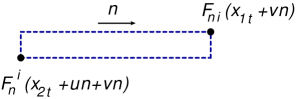
Figure 1: Gluon “Wilson frame” operator

$${\cal F}_{n}^{j}~{}(x_{1t},x_{2t})~{}\equiv~{}\int_{0}^{\infty}\!\!du~{}u^{1-j}{\cal F}_{n}(u;x_{1t},x_{2t}),$$

$${\cal F}_{n}(u;x_{1t},x_{2t})~{}\equiv~{}\int\!dv~{}2{\rm Tr}\big{\{}F_{n\xi}(x_{1t}+un+vn)[un+vn+x_{1t},vn+x_{1t}]$$

$$\hskip 68.2866pt\times~{}[vn+x_{1t},vn+x_{2t}]F_{n}^{~{}\xi}(x_{2t}+vn)[x_{2t}+vn,x_{2t}+un+vn]\big{\}}.$$ (25)

As $x_{1t}\rightarrow x_{2t}$ the Wilson-frame operator ${\cal F}_{n}(l;x_{1t},x_{2t})$ reduces to LR operator ${\cal F}(l,x_{1t})$ defined in Eq. (16). Moreover, it is intuitively clear that the point splitting $x_{12_{t}}$ serves as an UV cutoff for the light-ray operator in this limit, at least in the leading log approximation.

One can define also gluino and scalar “Wilson frames” by similar formulas and write down combinations but, as we mentioned above, we do not need their explicit form since at small $\omega$’s everything is determined by gluon operators ${\cal F}^{j}$. Thus, we define Wilson-frame operators (25) stretched in $n_{1}$, $n_{2}$ or $n_{3}$ directions and calculate their correlator at small $\omega_{i}$

It should be emphasized that narrow Wilson-frame operators are approximately conformally invariant: if one makes the inversion around the point $(0,0,0,a_{t})$ one gets the long and narrow Wilson frame with somewhat distorted ends, see Fig. 2.

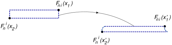
Figure 2: Transformation of Wilson frame under inversion $x_{\mu}\rightarrow x_{\mu}/x^{2}$

However, since we are calculating the correlators of Wilson frames in the leading BFKL approximation, the logarithmic integrals are determined by the whole range of integration over $u$ and small corrections at the fringes can be neglected in the leading-log approximation. Thus, one should expect the conformal formulas for the two- and three- point correlators of Wilson frames in the limit of small width of frames of the same form as Eqs. (18) and (19).

$$\big{\langle}{\cal F}_{n_{1}}^{j}\big{(}z_{t}+{w_{t}\over 2},z_{t}-{w_{t}\over 2}\big{)}{\cal F}_{n_{2}}^{j^{\prime}}\big{(}z^{\prime}_{t}+{w^{\prime}_{t}\over 2},z^{\prime}_{t}-{w^{\prime}_{t}\over 2}\big{)}\big{\rangle}~{}\stackrel{{\scriptstyle w_{t},w^{\prime}_{t}\rightarrow 0}}{{=}}~{}\delta(\nu-\nu^{\prime}){C(\nu,\Delta)\over|z_{t}-z^{\prime}_{t}|^{2\Delta(j)}}|w_{t}w^{\prime}_{t}|^{\gamma(j)}$$

(26)

and

$$\big{\langle}{\cal F}_{n_{1}}^{j_{1}}\big{(}z_{1_{t}}+{w_{1_{t}}\over 2},z_{1_{t}}-{w_{1_{t}}\over 2}\big{)}{\cal F}_{n_{2}}^{j_{2}}\big{(}z_{2_{t}}+{w_{2_{t}}\over 2},z_{2_{t}}-{w_{2_{t}}\over 2}\big{)}{\cal F}_{n_{3}}^{j_{3}}\big{(}z_{3_{t}}+{w_{3_{t}}\over 2},z_{3_{t}}-{w_{3_{t}}\over 2}\big{)}\big{\rangle}$$ (27)

$$\stackrel{{\scriptstyle w_{i_{t}}\rightarrow 0}}{{=}}~{}C(\Delta_{i},j_{i}){s_{12}^{j_{1}+j_{2}-j_{3}-1\over 2}|w_{1_{t}}|^{\gamma(j_{1})}\over|z_{12_{t}}|^{\Delta(j_{1})+\Delta(j_{2})-\Delta(j_{3})-1}}{s_{13}^{j_{1}+j_{3}-j_{2}-1\over 2}|w_{2_{t}}|^{\gamma(j_{2})}\over|z_{13_{t}}|^{\Delta(j_{1})+\Delta(j_{3})-\Delta(j_{2})-1}}{s_{23}^{j_{2}+j_{3}-j_{1}-1\over 2}|w_{3_{t}}|^{\gamma(j_{3})}\over|z_{23_{t}}|^{\Delta(j_{2})+\Delta(j_{3})-\Delta(j_{1})-1}}$$

with point-splitting distances $w_{t}$ serving as UV cutoffs similar to cutoff $\mu$ for the light-ray operators in Eqs. (18) and (19).

Our goal is the three-point formula (27) but first I remind the derivation of the BFKL asymptotics of two-point correlator (26) obtained in Ref. Balitsky:2013npa which will serve as a building block for three-frame calculation.

5 Correlator of two Wilson frames in the BFKL limit

The CF of two Wilson-frame operators in Regge kinematics is calculated in the same way as four-point correlator of local operators $\langle T\{{\cal O}(x_{1}){\cal O}(x_{2}){\cal O}(y_{1}){\cal O}(y_{2})\}\rangle$ in the Regge limit $x_{1n_{1}},y_{1n_{2}}\rightarrow\infty$, $x_{2n_{1}},y_{2n_{2}}\rightarrow-\infty$ and the rest of coordinates fixed. (Hereafter I use the notation $x_{n}\equiv x\cdot n$). Let me remind the essential steps of such calculation (see e.g. Ref. Balitsky:2009yp ).

5.1 Rapidity factorization for 4-point correlators in the Regge limit.

Let us consider the correlator of four scalar operators

$$A(x_{1},x_{2},x_{3},x_{4})~{}\equiv~{}\mu^{-4}(\mu^{4}x_{12}^{2}x_{34}^{2})^{2+\gamma_{o}}\langle T\{{\cal O}(x_{1}){\cal O}(x_{2}){\cal O}(x_{3}){\cal O}(x_{4})\}\rangle~{}$$

$$x_{1}=u_{1}n_{1}+x_{1_{\perp}},~{}~{}~{}x_{2}=v_{1}n_{1}+x_{2_{\perp}},~{}~{}~{}x_{3}=u_{2}n_{2}+x_{1_{\perp}},~{}~{}~{}x_{4}=v_{2}n_{2}+x_{4_{\perp}}$$ (28)

where $\gamma_{o}$ is the anomalous dimension of ${\cal O}$. In the Regge limit $s_{12}=-2n_{1}\cdot n_{2}\rightarrow\infty$ and $x_{i_{\perp}}$ fixed. The amplitude (28) is a function of two conformal ratios which can be chosen in the Regge limit as

$$R~{}=~{}{x_{13}^{2}x_{24}^{2}\over x_{12}^{2}x_{34}^{2}}~{}\simeq~{}{u_{1}u_{2}v_{1}v_{2}s_{12}^{2}\over x_{12_{t}}^{2}x_{34_{t}}^{2}},~{}~{}~{}~{}~{}~{}$$

$$r~{}=~{}R\Big{[}1-{x_{14}^{2}x_{23}^{2}\over x_{13}^{2}x_{24}^{2}}+{1\over R}\Big{]}^{2}~{}\simeq~{}{(u_{1}u_{2}x_{34_{\perp}}^{2}+v_{1}v_{2}x_{12_{\perp}}^{2}-u_{1}v_{2}x_{23_{\perp}}^{2}-v_{1}u_{2}x_{14_{\perp}}^{2})^{2}\over u_{1}u_{2}v_{1}v_{2}x_{12_{t}}^{2}x_{34_{\perp}}^{2}}$$ (29)

so that $R$ increases with “energy” $s_{12}=-2n_{1}\cdot n_{2}$ while $r$ is energy-independent. This corresponds to the momentum-space definition of Regge limit $s/m_{\perp}^{2}\gg 1$ where $m_{\perp}^{2}$ is a characteristic mass scale of the process, in our case the scale of inverse characteristic transverse distances.

In general, the calculation of particle scattering in the Regge limit is based on the rapidity factorization of the amplitude into the product of “projectile impact factor” with rapidities close to those of the projectile particle, “target impact factor” with rapidities close to the those of the target, and scattering of color dipoles encompassing the rapidities in the region between projectile and the target.

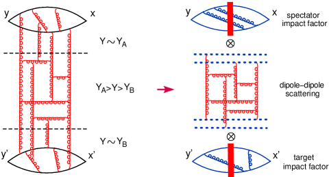
Figure 3: Rapidity factorization for 4-point correlator in the Regge limit

Technically, one expands the $T\{{\cal O}(x_{1}){\cal O}(x_{2})\}$ in the set of Wilson-line operators with the first being so-called “color dipole” ${\cal U}(z_{1_{\perp}},z_{2_{\perp}})$

$$T\{{\cal O}(x_{1}){\cal O}(x_{2})\}~{}=~{}\int\!d^{2}z_{1_{\perp}}d^{2}z_{2_{\perp}}~{}I(x_{1},x_{2};z_{1_{\perp}},z_{2_{\perp}}){\rm Tr}\{U(z_{1_{\perp}})U^{\dagger}(z_{2_{\perp}})\}+...$$

$${\cal U}(z_{1_{\perp}},z_{2_{\perp}})~{}\equiv~{}1-{1\over N_{c}}{\rm Tr}\{U(z_{1_{\perp}})U^{\dagger}(z_{2_{\perp}})\}$$ (30)

where integration goes over $z_{\perp}$ orthogonal to both $n_{1}$ and $n_{2}$, the Wilson line $U$ is defined as

$$U(z_{\perp})~{}\equiv~{}[\infty n_{1}+z_{\perp},-\infty n_{1}+z_{\perp}]$$ (31)

and dots stand for higher orders of perturbation theory and more Wilson lines. The rapidities inside the color dipole should be cut from above by characteristic rapidities in the integrals forming the impact factor. To ensure conformal invariance of the rapidity factorization, one should expand in “ composite conformal dipoles” introduced in Ref. Balitsky:2009xg .

$$T\{{\cal O}(x_{1}){\cal O}(x_{2})\}~{}=~{}\int\!d^{2}z_{1_{\perp}}d^{2}z_{2_{\perp}}~{}I(x_{1},x_{2};z_{1_{\perp}},z_{2_{\perp}}){\cal U}_{\rm conf}^{Y_{A}}(z_{1},z_{2})+...$$ (32)

where

$${\cal U}_{\rm conf}^{Y}(z_{1},z_{2})~{}=~{}1-{1\over N_{c}}{\rm Tr}\{U(z_{1_{\perp}})U^{\dagger}(z_{2_{\perp}})\}~{}+~{}\alpha_{s}\times~{}({\rm four~{}Wilson~{}lines~{}correction})$$ (33)

is a conformal composite dipole and $Y_{A}={1\over 2}\ln{4x_{1n_{2}}x_{2n_{2}}\over s_{12}x_{12_{t}}^{2}}$ is the conformally invariant rapidity cutoff. The explicit form of the 4-lines correction is presented in Ref. Balitsky:2009xg , but we do not need it for the leading BFKL logs.

Since we are interested in Regge asymptotics, it is sufficient to consider highest eigenvalue of BFKL intercept with spin 0. Defining a projection of the conformal dipole (33) on Lipatov’s eigenfunctions Lipatov:1985uk with spin 0, we get

$${\cal U}_{\rm conf}^{Y}(\nu,z_{0})~{}\equiv~{}{1\over\pi^{2}}\!\int\!{d^{2}z_{1}d^{2}z_{2}\over z_{12}^{4}}~{}\Big{(}{z_{12}^{2}\over z_{10}^{2}z_{20}^{2}}\Big{)}^{{1\over 2}-i\nu}~{}{\cal U}_{\rm conf}^{Y}(z_{1},z_{2})$$

$${\cal U}_{\rm conf}^{Y}(z_{1},z_{2})~{}=~{}\!\int_{-\infty}^{\infty}\!d\nu~{}{\nu^{2}\over\pi^{2}}\!\int\!d^{2}z_{0}\Big{(}{z_{12}^{2}\over z_{10}^{2}z_{20}^{2}}\Big{)}^{{1\over 2}+i\nu}{\cal U}_{\rm conf}^{Y}(\nu,z_{0})~{}~{}+~{}{\rm higher~{}spins}$$ (34)

and therefore one can rewrite Eq. (32) as follows

$$T\{{\cal O}(x_{1}){\cal O}(x_{2})\}~{}=~{}\int\!d^{2}z_{0}\!\int\!d\nu~{}I_{A}(\nu)\bigg{[}{x_{12}^{2}x_{1n_{2}}x_{2n_{2}}\over{(x_{1}-z_{0})_{\perp}^{2}\over x_{1n_{2}}}-{(x_{2}-z_{0})_{\perp}^{2}\over x_{2n_{2}}}}\bigg{]}^{{1\over 2}+i\nu}{\cal U}_{\rm conf}^{Y_{A}}(\nu,z_{0}).$$ (35)

Repeating the same expansion for the “target” we get

$$T\{{\cal O}(x_{3}){\cal O}(x_{4})\}~{}=~{}\int\!d^{2}z_{0}\!\int\!d\nu~{}I_{A}(\nu)\bigg{[}{x_{34}^{2}x_{3n_{1}}x_{4n_{1}}\over{(x_{3}-z_{0})_{\perp}^{2}\over x_{3n_{1}}}-{(x_{4}-z_{0})_{\perp}^{2}\over x_{4n_{1}}}}\bigg{]}^{{1\over 2}+i\nu}{\cal V}_{\rm conf}^{Y_{B}}(\nu,z_{0}).$$ (36)

where $Y_{B}={1\over 2}\ln{4x_{3n_{1}}x_{4n_{1}}\over s_{12}x_{34_{\perp}}^{2}}$ and the conformal dipole ${\cal V}_{\rm conf}^{Y_{B}}(\nu,z_{0})$ is defined as

$${\cal V}_{\rm conf}^{Y_{B}}(\nu,z_{0})~{}\equiv~{}{1\over\pi^{2}}\!\int\!{d^{2}z_{3}d^{2}z_{4}\over z_{34}^{4}}~{}\Big{(}{z_{34}^{2}\over z_{30}^{2}z_{40}^{2}}\Big{)}^{{1\over 2}-i\nu}~{}{\cal V}_{\rm conf}^{Y_{B}}(z_{3},z_{4})$$

$${\cal V}_{\rm conf}^{Y_{B}}(z_{3_{\perp}},z_{4_{\perp}})~{}\equiv~{}1-{1\over N_{c}}{\rm Tr}\{V(z_{3_{\perp}})V^{\dagger}(z_{4_{\perp}})\}_{\rm conf}^{Y_{B}}$$ (37)

where Wilson lines $V$ are ordered along $n_{2}$ direction

$$V(z_{\perp})~{}\equiv~{}[\infty n_{2}+z_{\perp},-\infty n_{2}+z_{\perp}]$$ (38)

Now the 4-point CF can be represented as an integral of the product of two impact factors $I_{A}(\nu),~{}I_{B}(\nu^{\prime})$ and the amplitude of scattering of two color dipoles. In the leading BFKL approximation this amplitude has the form ($\alpha_{s}\equiv{g_{{}_{\rm YM}}^{2}\over 4\pi}$)

$$\langle{\cal U}_{\rm conf}^{Y_{A}}(\nu,z_{0}){\cal V}_{\rm conf}^{Y_{B}}(\nu^{\prime},z^{\prime}_{0})\rangle~{}=~{}-{\alpha_{s}^{2}(N_{c}^{2}-1)\over 4N_{c}^{2}}e^{\aleph(\nu,g^{2})\ln Y_{A}Y_{B}}$$ (39)

$$\times~{}{16\pi^{2}\over\nu^{2}(1+4\nu^{2})^{2}}\Big{[}\delta(z_{0}-z^{\prime}_{0})\delta(\nu+\nu^{\prime})+{2^{1-4i\nu}\delta(\nu-\nu^{\prime})\over\pi|z_{0}-z^{\prime}_{0}|^{2-4i\nu}}{\Gamma\big{(}{1\over 2}+i\nu\big{)}\Gamma(1-i\nu)\over\Gamma(i\nu)\Gamma\big{(}{1\over 2}-i\nu\big{)}}\Big{]}.$$

where

$$\aleph(\nu,g^{2})~{}=~{}4g^{2}\big{[}2\psi(1)-\psi\big{(}{1\over 2}+i\nu\big{)}-\psi\big{(}{1\over 2}-i\nu\big{)}\big{]}~{}+~{}O(g^{4})$$ (40)

is the pomeron intercept (22).

As I mentioned in the Introduction, in QCD only the $\alpha_{s}^{2}$ correction is known Fadin:1998py while in ${\cal N}=4$ SYM the $g^{6}$ term is known analytically Gromov:2015vua ; Velizhanin:2015xsa ; Caron-Huot:2016tzz and many more can be calculated numerically Gromov:2015vua using Quantum Spectral Curve method Alfimov:2014bwa .

Assembling the result for the 4-point CF(28) one gets the result in the form of general formula Cornalba:2007fs for correlators in the “Regge + large $N_{c}$” limit

$$A(x_{i})~{}\stackrel{{\scriptstyle s_{12}\rightarrow\infty}}{{=}}~{}{i\over 2}\!\int\!d\nu~{}f_{+}(\aleph(g^{2},\nu))F(g^{2},\nu)\Omega(r,\nu)R^{\aleph(g^{2},\nu)/2}$$ (41)

where $f_{+}(\aleph)={e^{i\pi\aleph}-1\over\sin\pi\aleph}$ is a signature factor and

$$\Omega(r,\nu)~{}=~{}{\nu\over 2\pi^{2}}{\sin 2\nu\rho\over\sinh\rho},~{}~{}~{}~{}\cosh\rho={\sqrt{r}\over 2}$$ (42)

is a solution of the Laplace equation in $H_{3}$ hyperboloid $(\partial^{2}_{H_{3}}+\nu^{2}+1)\Omega(r,\nu)=0$. The dynamics is described by the pomeron intercept $\aleph(g^{2},\nu)$ and the “pomeron residue” $F(g^{2},\nu)$. The formula (41) was proved in Cornalba:2007fs (see also Costa:2012cb ) by considering the leading Regge pole in a conformal theory. Also, it was demonstrated up to the NLO level that the structure (41) is reproduced by the high-energy OPE in Wilson lines Balitsky:1995ub ; Balitsky:1998ya ; Balitsky:2001gj .

5.2 Correlator of two Wilson frames in the Regge limit

The Regge limit for CF of two Wilson-frame operators means that longitudinal length of frame is much greater than the transverse separation between the frames and the width of frames is even less. As we mentioned, at small frame widths the frames are approximately conformally invariant so one may expect that the general formula (41) is applicable. At $x_{12}^{2},x_{34}^{2}\rightarrow 0$ one gets

$$r~{}\rightarrow~{}{(u_{1}-v_{1})^{2}(u_{2}-v_{2})^{2}x_{13_{\perp}}^{4}\over u_{1}v_{1}u_{2}v_{2}x_{12_{\perp}}^{2}x_{34_{\perp}}^{2}}$$ (43)

and

$$\Omega(r,\nu)~{}\rightarrow~{}{\nu\over 2\pi^{2}i}\big{(}r^{-{1\over 2}+i\nu}-r^{-{1\over 2}-i\nu}\big{)}$$ (44)

Moreover, if we consider “forward” correlation function

$$A(l,l^{\prime};x_{1_{\perp}},x_{2_{\perp}},x_{3_{\perp}},x_{4_{\perp}})~{}$$ (45)

$$\equiv~{}\int_{0}^{\infty}\!dv_{1}dv_{2}~{}A(ln_{1}+v_{1}n_{1}+x_{1_{\perp}},v_{1}n_{1}+x_{2_{\perp}},l^{\prime}n_{2}+v_{2}n_{2}+x_{3_{\perp}},v_{2}n_{2}+x_{4_{\perp}})$$

the Eq. (41) reduces to

$$A(l,l^{\prime};x_{1_{\perp}},x_{2_{\perp}},x_{3_{\perp}},x_{4_{\perp}})~{}\stackrel{{\scriptstyle x_{12_{\perp}}^{2},x_{34_{\perp}}^{2}\rightarrow 0}}{{=}}~{}ll^{\prime}i\!\int\!{d\nu}~{}\Phi(\nu,g^{2})$$ (46)

$$\hskip 105.27519pt\times~{}\Big{(}{x_{12_{\perp}}^{2}x_{34\perp}^{2}\over x_{13_{\perp}}^{4}}\Big{)}^{{1\over 2}+i\nu}\Big{(}{l^{2}{l^{\prime}}^{2}\over x_{12_{\perp}}^{2}x_{34\perp}^{2}}\Big{)}^{\aleph(\nu,g^{2})/2}f_{+}(\aleph)~{}$$

As noted in Sect. 4, at small widths Wilson frames are approximately conformally invariant so we need to obtain the representation of Eq. (46) type for the correlator

$$\langle{\cal F}_{n_{1}}\big{(}l;z_{t}+{w_{t}\over 2},z_{t}-{w_{t}\over 2}\big{)}{\cal F}_{n_{2}}\big{(}l^{\prime};z^{\prime}_{t}+{w^{\prime}_{t}\over 2},z^{\prime}_{t}-{w^{\prime}_{t}\over 2}\big{)}\rangle$$ (47)

at $l,l^{\prime}\rightarrow\infty$ (which corresponds to $j\rightarrow 1\Leftrightarrow\omega\rightarrow 0$ after integration over $l,l^{\prime}$). In Ref. Balitsky:2013npa we performed calculation of CF of two Wilson-frame operators

$$\langle{\cal F}_{n_{1}}\big{(}l;z_{t}+{w_{t}\over 2},z_{t}-{w_{t}\over 2}\big{)}{\cal F}_{n_{2}}\big{(}l^{\prime};z^{\prime}_{t}+{w^{\prime}_{t}\over 2},z^{\prime}_{t}-{w^{\prime}_{t}\over 2}\big{)}\rangle$$ (48)

in Regge kinematics in the same way as four-point correlator of local operators. In this Section I’ll reproduce that calculation in a slightly different way useful for considering 3-frame correlator in the next Section.

We introduce some “rapidity divide” $Y_{0}$ between $Y_{A}$ and $Y_{B}$ and integrate between $Y_{A}$ and $Y_{0}$ and between $Y_{0}$ and $Y_{B}$ in the leading BFKL approximation. After that, we need to convolute the results with the leading order dipole-dipole scattering amplitude.

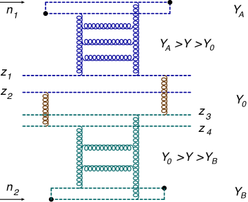
Figure 4: Correlator of two Wilson frames in the Regge limit

The first step is the expansion of Wilson frame in color dipoles. The impact factor for Wilson frame, i.e. the coefficient of expansion of “Wilson frame” in color dipoles was calculated in Ref. Balitsky:2013npa

$${\cal F}_{n}(l;x_{\perp},y_{\perp})~{}=~{}{N_{c}^{2}\over 4\pi^{3}l}\!\int\!d^{2}z_{\perp}~{}\big{\{}1-{\cal U}(x_{\perp},z_{\perp})-{\cal U}(z_{\perp},y_{\perp})$$ (49)

$$\hskip 19.91692pt+~{}{\cal U}(x_{\perp},z_{\perp}){\cal U}(z_{\perp},y_{\perp})~{}+~{}O\big{(}{1\over N_{c}}\big{)}\big{\}}^{Y_{A}}\Big{[}{2\over(x-z)_{\perp}^{2}(y-z)_{\perp}^{2}}-{4(x-z,y-z)_{\perp}^{2})\over(x-z)_{\perp}^{4}(y-z)_{\perp}^{4}}\Big{]}$$

where the rapidity cutoff is

$$Y_{A}={1\over 2}\ln{l^{2}s_{12}\over(x-y)_{\perp}^{2}}$$ (50)

by analogy with four-point correlator. As explained in Ref. Balitsky:2013npa , in order to calculate the correlator of two Wilson frames we need to take into account only the linear terms in Eq. (49) so we can neglect the last quadratic term. To get the evolution of dipoles in Eq. (49) from $Y_{A}$ to $Y_{0}$ we project onto Lipatov’s eigenfunctions, i.e.. rewrite in terms of conformal dipoles and evolve these conformal dipoles in the leading BFKL order.

The projection of Eq. (49) on Lipatov’s eigenfunctions with spin 0 reads

$${\cal F}_{n}(l;x_{\perp},y_{\perp})$$ (51)

$$=~{}-{N_{c}^{2}\over 4\pi^{3}l}\!\int\!d\nu~{}{\nu^{2}\over\pi^{2}}\!\int\!d^{2}z_{0}~{}{\cal U}_{\rm conf}^{a}(\nu,z_{0})\!\int\!d^{2}z_{\perp}\Big{[}{2\over(x-z)_{\perp}^{2}(y-z)_{\perp}^{2}}-{4(x-z,y-z)_{\perp}^{2})\over(x-z)_{\perp}^{4}(y-z)_{\perp}^{4}}\Big{]}$$

$$\hskip 62.59605pt\times~{}\Big{[}\Big{(}{(x-z)_{\perp}^{2}\over(x-z_{0})_{\perp}^{2}(z-z_{0})_{\perp}^{2}}\Big{)}^{{1\over 2}+i\nu}+\Big{(}{(y-z)_{\perp}^{2}\over(y-z_{0})_{\perp}^{2}(z-z_{0})_{\perp}^{2}}\Big{)}^{{1\over 2}+i\nu}\Big{]}$$

$$=~{}{N_{c}\over\pi^{2}l}\!\int\!d\nu~{}{\nu^{2}\over\pi^{2}}{{1\over 2}+i\nu\over{1\over 2}-i\nu}\!\int\!d^{2}z_{0}~{}\Big{[}{2(x-z_{0},y-z_{0})_{\perp}^{2}\over(x-z_{0})_{\perp}^{2}(y-z_{0})_{\perp}^{2}}-1\Big{]}{[(x-y)_{\perp}^{2}]^{-{1\over 2}+i\nu}{\cal U}_{\rm conf}(\nu,z_{0})^{Y_{A}}\over[(x-z_{0})_{\perp}^{2}]^{{1\over 2}+i\nu}[(y-z_{0})_{\perp}^{2}]^{{1\over 2}+i\nu}}$$

where we used Eq. (4.11) from Ref. Balitsky:2013npa to get the last line.

Moreover, in the limit of narrow Wilson frame $(x-y)_{\perp}\rightarrow 0$ the integral in the r.h.s. of the above equation can be simplified. Using Eqs. (C.4) and (C.6) from Ref. Balitsky:2013npa one easily obtains

$$\!\int\!d^{2}z_{0}~{}\Big{[}{2(x-z_{0},y-z_{0})_{\perp}^{2}\over(x-z_{0})_{\perp}^{2}(y-z_{0})_{\perp}^{2}}-1\Big{]}{[(x-y)_{\perp}^{2}]^{{1\over 2}+i\nu}\over[(x-z_{0})_{\perp}^{2}]^{{1\over 2}+i\nu}[(y-z_{0})_{\perp}^{2}]^{{1\over 2}+i\nu}}\Big{(}{z_{12}^{2}\over z_{10}^{2}z_{20}^{2}}\Big{)}^{{1\over 2}-i\nu}~{}$$

$$\stackrel{{\scriptstyle x\rightarrow y}}{{=}}~{}{i\pi\over 2\nu}{\big{(}{1\over 2}-i\nu\big{)}^{2}\over\big{(}{1\over 2}+i\nu\big{)}^{2}}2^{4i\nu}{\Gamma\big{(}{1\over 2}-i\nu\big{)}\Gamma(i\nu)\over\Gamma\big{(}{1\over 2}+i\nu\big{)}\Gamma(-i\nu)}\Big{(}{|x-y|^{2}z_{12}^{2}\over(x-z_{1})^{2}(x-z_{2})^{2}}\Big{)}^{{1\over 2}-i\nu}$$

$$\hskip 93.89409pt-~{}{i\pi\over 2\nu}2^{-4i\nu}{\Gamma\big{(}{1\over 2}+i\nu\big{)}\Gamma(-i\nu)\over\Gamma\big{(}{1\over 2}-i\nu\big{)}\Gamma(i\nu)}\Big{(}{|x-y|^{2}z_{12}^{2}\over(x-z_{1})^{2}(x-z_{2})^{2}}\Big{)}^{{1\over 2}+i\nu}$$ (52)

Recalling the definition (34) of ${\cal U}_{\rm conf}$ and substituting Eq. (52) in Eq. (51) one gets

$${\cal F}_{n}\big{(}l;z_{t}+{w_{t}\over 2},z_{t}-{w_{t}\over 2}\big{)}~{}=~{}{iN_{c}^{2}\over\pi^{3}l}\int\!d\nu~{}\nu{2^{-4i\nu}\Gamma\big{(}{3\over 2}+i\nu\big{)}\Gamma(1-i\nu)\over\Gamma\big{(}{3\over 2}-i\nu\big{)}\Gamma(1+i\nu)}(w_{t}^{2})^{-{1\over 2}+i\nu}{\cal U}^{Y_{A}}_{\rm conf}(z_{t},-\nu)$$

(53)

The BFKL evolution of a conformal dipole reads

$${\cal U}_{\rm conf}^{Y_{A}}(\nu,z_{0})~{}=~{}e^{(Y_{A}-Y_{0})\aleph(\nu)}{\cal U}_{\rm conf}^{Y_{0}}(\nu,z_{0})$$ (54)

so the result of integration over rapidities in the region $Y_{A}>Y>Y_{0}$ is

$${\cal F}_{n_{1}}\big{(}l;z_{t}+{w_{t}\over 2},z_{t}-{w_{t}\over 2}\big{)}~{}$$

$$=~{}{iN_{c}^{2}\over\pi^{3}l}\int\!d\nu~{}\nu{2^{-4i\nu}\Gamma\big{(}{3\over 2}+i\nu\big{)}\Gamma(1-i\nu)\over\Gamma\big{(}{3\over 2}-i\nu\big{)}\Gamma(1+i\nu)}(w_{t}^{2})^{-{1\over 2}+i\nu}e^{(Y_{A}-Y_{0})\aleph(\nu,g^{2})}{\cal U}^{Y_{0}}_{\rm conf}(z_{t},-\nu)$$ (55)

where $Y_{A}=\ln l+{1\over 2}\ln{s_{12}\over w_{t}^{2}}$.

Repeating the same procedure for the bottom part of the diagram in Fig. 4 one obtains the result of integration over rapidities $Y_{0}>Y$ in the form

$${\cal F}_{n_{2}}\big{(}l^{\prime};z^{\prime}_{t}+{w^{\prime}_{t}\over 2},z^{\prime}_{t}-{w^{\prime}_{t}\over 2}\big{)}~{}$$ (56)

$$=~{}{iN_{c}^{2}\over\pi^{3}l^{\prime}}\int\!d\nu^{\prime}~{}\nu^{\prime}{2^{-4i\nu^{\prime}}\Gamma\big{(}{3\over 2}+i\nu^{\prime}\big{)}\Gamma(1-i\nu^{\prime})\over\Gamma\big{(}{3\over 2}-i\nu^{\prime}\big{)}\Gamma(1+i\nu^{\prime})}({w^{\prime}}_{t}^{2})^{-{1\over 2}+i\nu^{\prime}}e^{(Y_{0}+Y_{B})\aleph(\nu^{\prime},g^{2})}{\cal V}^{Y_{0}}_{\rm conf}(z^{\prime}_{t},-\nu^{\prime})$$

where $Y_{B}=\ln l^{\prime}+{1\over 2}\ln{s_{12}\over{w^{\prime}}_{t}^{2}}$.

Using now the result for scattering of color dipoles in the leading perturbative order

$$\langle{\cal U}_{\rm conf}^{Y_{0}}(-\nu,z_{0}){\cal V}_{\rm conf}^{Y_{0}}(-\nu^{\prime},z^{\prime}_{0})\rangle~{}$$ (57)

$$=~{}-\alpha_{s}^{2}{4\pi^{2}\big{(}1-{1\over N_{c}^{2}}\big{)}\over\nu^{2}(1+4\nu^{2})^{2}}\Big{[}\delta(z_{0}-z^{\prime}_{0})\delta(\nu+\nu^{\prime})-i\nu{2^{1+4i\nu}\delta(\nu-\nu^{\prime})\over\pi|z_{0}-z^{\prime}_{0}|^{2+4i\nu}}{\Gamma\big{(}{1\over 2}-i\nu\big{)}\Gamma(1+i\nu)\over\Gamma(1-i\nu)\Gamma\big{(}{1\over 2}+i\nu\big{)}}\Big{]}.$$

we get the result for correlator of two Wilson frames in the form of Eq. (46) type

$$\langle{\cal F}_{n_{1}}\big{(}l;z_{t}+{w_{t}\over 2},z_{t}-{w_{t}\over 2}\big{)}{\cal F}_{n_{2}}\big{(}l^{\prime};z^{\prime}_{t}+{w^{\prime}_{t}\over 2},z^{\prime}_{t}-{w^{\prime}_{t}\over 2}\big{)}\rangle$$

$$=~{}-i{g^{2}N_{c}^{2}\over\pi^{3}ll^{\prime}}\int\!d\nu~{}{2^{3-4i\nu}\nu\over\big{(}{1\over 2}+i\nu\big{)}\big{(}{1\over 2}-i\nu\big{)}^{3}}{\Gamma\big{(}{3\over 2}+i\nu\big{)}\Gamma(1-i\nu)\over\Gamma\big{(}{3\over 2}-i\nu\big{)}\Gamma(1+i\nu)}{(w_{t}^{2}{w^{\prime}}_{t}^{2})^{-{1\over 2}+i\nu}e^{(Y_{A}+Y_{B})\aleph(\nu,g^{2})}\over([z_{t}-z^{\prime}_{t})^{2}]^{1+2i\nu}}$$

$$=~{}-i{g^{2}N_{c}^{2}\over\pi^{3}ll^{\prime}}\int\!d\nu~{}{2^{3-4i\nu}\nu(ll^{\prime}s_{12})^{\aleph(\nu)}\over\big{(}{1\over 2}+i\nu\big{)}\big{(}{1\over 2}-i\nu\big{)}^{3}}{\Gamma\big{(}{3\over 2}+i\nu\big{)}\Gamma(1-i\nu)\over\Gamma\big{(}{3\over 2}-i\nu\big{)}\Gamma(1+i\nu)}{(w_{t}^{2}{w^{\prime}}_{t}^{2})^{-{1\over 2}+i\nu-{1\over 2}\aleph(\nu,g^{2})}\over[(z_{t}-z^{\prime}_{t})^{2}]^{1+2i\nu}}$$ (58)

Note that the “rapidity divide” $Y_{0}$ disappeared from the result. Moreover, the scattering amplitude (58) depends only on product of $l$ and $l^{\prime}$ which is a reflection of boost invariance of the original amplitude (25): it is easy to see that if one makes boost $n_{1}\rightarrow\lambda n_{1}$ and $n_{2}\rightarrow{1\over\lambda}n_{2}$ the correlator (25) does not change. Now we shall see that this property leads to the $\delta$-function in the correlator (26).

Indeed, the integral over $l$ and $l^{\prime}$ have the form

$$\langle{\cal F}^{j}_{n_{1}}\big{(}z_{t}+{w_{t}\over 2},z_{t}-{w_{t}\over 2}\big{)}{\cal F}^{j^{\prime}}_{n_{2}}\big{(}z^{\prime}_{t}+{w^{\prime}_{t}\over 2},z^{\prime}_{t}-{w^{\prime}_{t}\over 2}\big{)}\rangle~{}=~{}-i{g^{2}N_{c}^{2}\over\pi^{3}}\!\int_{0}^{\infty}\!dldl^{\prime}~{}l^{-j}{l^{\prime}}^{-j^{\prime}}$$ (59)

$$\times~{}\theta\Big{(}ll^{\prime}-{(z_{t}-z^{\prime}_{t})^{2}\over s_{12}}\Big{)}\int\!d\nu~{}{\nu 2^{3-4i\nu}(ll^{\prime}s_{12})^{\aleph(\nu,g^{2})}\over\big{(}{1\over 2}+i\nu\big{)}\big{(}{1\over 2}-i\nu\big{)}^{3}}{\Gamma\big{(}{3\over 2}+i\nu\big{)}\Gamma(1-i\nu)\over\Gamma\big{(}{3\over 2}-i\nu\big{)}\Gamma(1+i\nu)}{(w_{t}^{2}{w^{\prime}}_{t}^{2})^{-{1\over 2}+i\nu-{1\over 2}\aleph(\nu,g^{2})}\over[(z_{t}-z^{\prime}_{t})^{2}]^{1+2i\nu}}$$

where the factor $\theta\big{(}ll^{\prime}-{(z_{t}-z^{\prime}_{t})^{2}\over s_{12}}\big{)}$ comes from the restriction that the longitudinal size of two Wilson frames should be greater than the relative transverse separation.

Performing the integration over $l$ and $l^{\prime}$ one obtains where $j={1\over 2}+i\varsigma$ and $j^{\prime}={1\over 2}+i\varsigma^{\prime}$.

$$\langle{\cal F}^{j}_{n_{1}}\big{(}z_{t}+{w_{t}\over 2},z_{t}-{w_{t}\over 2}\big{)}{\cal F}^{j^{\prime}}_{n_{2}}\big{(}z^{\prime}_{t}+{w^{\prime}_{t}\over 2},z^{\prime}_{t}-{w^{\prime}_{t}\over 2}\big{)}\rangle~{}=~{}-i\delta(\varsigma-\varsigma^{\prime}){g^{2}N_{c}^{2}\over\pi^{2}}\!\int_{-\infty}^{\infty}\!d\nu~{}{1\over\omega-\aleph(\nu,g^{2})}$$

$$\times~{}{\nu 2^{4-4i\nu}s_{12}^{\omega}\over\big{(}{1\over 2}+i\nu\big{)}\big{(}{1\over 2}-i\nu\big{)}^{3}}{\Gamma\big{(}{3\over 2}+i\nu\big{)}\Gamma(1-i\nu)\over\Gamma\big{(}{3\over 2}-i\nu\big{)}\Gamma(1+i\nu)}{(w_{t}^{2}{w^{\prime}}_{t}^{2})^{-{1\over 2}+i\nu-{1\over 2}\aleph(\nu,g^{2})}\over[(z_{t}-z^{\prime}_{t})^{2}]^{j+2i\nu-\aleph(\nu,g^{2})}}$$ (60)

Next, we analytically continue this formula to small $\omega=j-1$. To estimate this integral at small $\omega$’s it is convenient to rewrite it in the variable $\xi=2i\nu-1$.

$$\langle{\cal F}^{j}_{n_{1}}\big{(}z_{t}+{w_{t}\over 2},z_{t}-{w_{t}\over 2}\big{)}{\cal F}^{j^{\prime}}_{n_{2}}\big{(}z^{\prime}_{t}+{w^{\prime}_{t}\over 2},z^{\prime}_{t}-{w^{\prime}_{t}\over 2}\big{)}\rangle~{}=~{}\delta(\varsigma-\varsigma^{\prime})g^{4}N_{c}^{2}\!\int_{-1-i\infty}^{-1+i\infty}\!{d\xi\over 2\pi i}~{}{1\over\omega-\tilde{\aleph}(\xi,g^{2})}$$

$$\times~{}{2^{5-2\xi}\pi s_{12}^{\omega}\over\xi^{2}\sin\pi\xi\Gamma^{2}\big{(}1-{\xi\over 2}\big{)}\Gamma^{2}\big{(}{1\over 2}+{\xi\over 2}\big{)}}{(w_{t}^{2}{w^{\prime}}_{t}^{2})^{\xi-\tilde{\aleph}(\xi,g^{2})\over 2}\over[(z_{t}-z^{\prime}_{t})^{2}]^{2+\omega+\xi-\tilde{\aleph}(\xi,g^{2})}}$$ (61)

The notation here is

$$\tilde{\aleph}(\xi,g^{2})~{}\equiv~{}\aleph\big{(}-i{1+\xi\over 2},g^{2}\big{)}~{}=~{}4g^{2}\big{[}2\psi(1)-\psi\big{(}-{\xi\over 2}\big{)}-\psi\big{(}1+{\xi\over 2}\big{)}\big{]}~{}+~{}O(g^{4})$$ (62)

and we often omit the $g^{2}$ dependence to avoid cluttering of the formulas.

At small $w_{t}^{2},{w^{\prime}}_{t}^{2}$ we can close the contour of $\xi$ integration on the residues in the right half-plane. The two leading poles are located at $\xi^{\ast}=\tilde{\aleph}^{-1}(\omega)$ and $\xi=0$. Let us consider them in turn. Taking residue at $\xi^{\ast}=\tilde{\aleph}^{-1}(\omega,g^{2})$ we get

$$\langle{\cal F}^{j}_{n_{1}}\big{(}z_{t}+{w_{t}\over 2},z_{t}-{w_{t}\over 2}\big{)}{\cal F}^{j^{\prime}}_{n_{2}}\big{(}z^{\prime}_{t}+{w^{\prime}_{t}\over 2},z^{\prime}_{t}-{w^{\prime}_{t}\over 2}\big{)}\rangle$$

$$=~{}\delta(\varsigma-\varsigma^{\prime})g^{2}N_{c}^{2}{2^{5-2\xi^{\ast}}\pi s_{12}^{\omega}\over{\xi^{\ast}}^{2}\sin\pi\xi^{\ast}\Gamma^{2}\big{(}1-{\xi^{\ast}\over 2}\big{)}\Gamma^{2}\big{(}{1\over 2}+{\xi^{\ast}\over 2}\big{)}\aleph^{\prime}(\xi^{\ast})}{(w_{t}^{2}{w^{\prime}}_{t}^{2})^{\xi^{\ast}-\omega\over 2}\over[(z_{t}-z^{\prime}_{t})^{2}]^{2+\xi^{\ast}}}$$ (63)

Comparing this equation to general form of two-point correlator of light-ray operators (18) we see that $\xi^{\ast}-\omega$ can be identified with anomalous dimension $\gamma$ so we finally get Balitsky:2013npa

$$\langle{\cal F}^{j}_{n_{1}}\big{(}z_{t}+{w_{t}\over 2},z_{t}-{w_{t}\over 2}\big{)}{\cal F}^{j^{\prime}}_{n_{2}}\big{(}z^{\prime}_{t}+{w^{\prime}_{t}\over 2},z^{\prime}_{t}-{w^{\prime}_{t}\over 2}\big{)}\rangle$$

$$=~{}\delta(\varsigma-\varsigma^{\prime})g^{2}N_{c}^{2}{2^{5-2\xi^{\ast}}\pi s_{12}^{\omega}\over{\xi^{\ast}}^{2}\sin\pi\xi^{\ast}\Gamma^{2}\big{(}1-{\xi^{\ast}\over 2}\big{)}\Gamma^{2}\big{(}{1\over 2}+{\xi^{\ast}\over 2}\big{)}\aleph^{\prime}(\xi^{\ast})}{(w_{t}^{2}{w^{\prime}}_{t}^{2})^{\gamma^{\ast}\over 2}\over[(z_{t}-z^{\prime}_{t})^{2}]^{2+\omega+\gamma^{\ast}}}$$ (64)

where $\gamma^{\ast}$ is a solution of the equation (21) and $\xi^{\ast}=\gamma^{\ast}+\omega=\Delta-3$.

Note that this formula is actually at the NLO level: in the leading log approximation we just get $\omega=\aleph(\gamma^{\ast})$ and $[(z-z^{\prime})_{t}^{2}]^{-2-\gamma_{\ast}}$ in the r.h.s. of Eq. (64). The reason that we got the NLO equation (21) is that we used $Y_{A}=\ln l+{1\over 2}\ln s_{12}m_{\perp}^{2}-{1\over 2}\ln m_{\perp}^{2}w_{t}^{2}$ where the last term exceeds the LLA accuracy. As demonstrated in Ref. Balitsky:2013npa , we can do this using the exact formula for the 4-point correlator (41). Unfortunately, for the 6-point correlator there is no such formula so we cannot promote our LO BFKL calculation to the NLO level.

At $g^{2}\ll\omega\ll 1$ we get $\xi_{\ast}\simeq-8{g^{2}\over\omega}$ (recall that $\aleph(\xi)\simeq-8{g^{2}\over\xi}$ at small $\xi$) and therefore the result (64) takes the form

$$\langle{\cal F}^{j}_{n_{1}}\big{(}z_{t}+{w_{t}\over 2},z_{t}-{w_{t}\over 2}\big{)}{\cal F}^{j^{\prime}}_{n_{2}}\big{(}z^{\prime}_{t}+{w^{\prime}_{t}\over 2},z^{\prime}_{t}-{w^{\prime}_{t}\over 2}\big{)}\rangle$$

$$\simeq~{}-\delta(\omega-\omega^{\prime}){N_{c}^{2}\omega s_{12}^{\omega}\over 2\pi[(z_{t}-z^{\prime}_{t})^{2}]^{2+\omega}}\Big{(}{(z_{t}-z^{\prime}_{t})^{2}\over|w_{t}w^{\prime}_{t}|}\Big{)}^{{8g^{2}\over\omega}+\omega}$$ (65)

which agrees with Eq. (4.17) from Ref. Balitsky:2013npa .

Let us consider now the pole at $\xi=0$. At small $\xi$

$${1\over\omega-\tilde{\aleph}(\xi)}\simeq{\xi\over 8g^{2}}\Big{(}1-{\xi\omega\over 8g^{2}}+...\Big{)}$$ (66)

so the residue at $\xi=0$ yields

$$\delta(\omega-\omega^{\prime}){\omega s_{12}^{\omega}N_{c}^{2}\over 2\pi[(z_{t}-z^{\prime}_{t})^{2}]^{2+\omega}}\Big{[}1+{8g^{2}\over\omega}\ln{(z_{t}-z^{\prime}_{t})^{2}\over|w_{t}w^{\prime}_{t}|}\Big{]}$$ (67)

Thus, the result for diagrams in Fig. 4 is a sum of Eq. (64) and Eq. (67). However, there are two low-order diagrams shown in Fig. 5 that are not included in this result since the formula (49) is correct starting from the second order of perturbation theory.

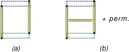
Figure 5: First (a) and second (b) order diagrams for the correlator of two Wilson frames

These diagrams should cancel the contribution of the $\xi=0$ pole (67) so the final result (64) has proper conformal behavior. The tree-level diagram in Fig. 5a is calculated in the appendix A and the result (131) is minus the first term in the square brackets in Eq. (67). Similarly, the contribution of diagrams in Fig. 5b should cancel the second term so the contribution of all diagrams (in Fig.5 and Fig. 4) is given by Eq. (64).

6 Correlator of three Wilson frames in the triple Regge limit

6.1 Triple BFKL evolution

To get the structure constant in Eq. (19) at $\omega_{i}\rightarrow 0$ we will consider the correlator of three gluon Wilson frames aligned along $n_{1}$, $n_{2}$, and $n_{3}$ directions:

$$\big{\langle}{\cal F}_{n_{1}}^{j_{1}}\big{(}z_{1_{t}}+{w_{1_{t}}\over 2},z_{1_{t}}-{w_{1_{t}}\over 2}\big{)}{\cal F}_{n_{2}}^{j_{2}}\big{(}z_{2_{t}}+{w_{2_{t}}\over 2},z_{2_{t}}-{w_{2_{t}}\over 2}\big{)}{\cal F}_{n_{3}}^{j_{3}}\big{(}z_{3_{t}}+{w_{3_{t}}\over 2},z_{3_{t}}-{w_{3_{t}}\over 2}\big{)}\big{\rangle}$$ (68)

A typical diagram is shown in Fig. 6.

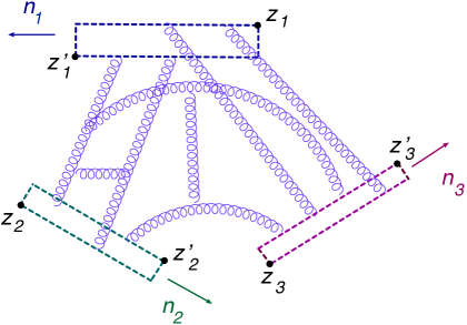
Figure 6: Correlator of three Wison frames

As usual, we assume that longitudinal lengths of frames are much greater than the transverse separations between the frames and those separations are much greater than widths of the frames. The form of the three-point correlators of light-ray operators (19) suggests that this correlator is determined by three BFKL evolutions. It will be demonstrated in this Section.

The method to obtain BFKL asymptotics of a scattering amplitude by evolution of Wilson lines is the following. In a typical amplitude like shown in Fig. 7a we separate the (gluon) fields according to their rapidity, using the fact that particles with different rapidities perceive each other as Wilson lines, and study the evolution of these Wilson lines with respect to rapidity cutoff. Since we have now three light-like directions, it is convenient to introduce “triple Sudakov variables”

$$k=\alpha n_{1}+\beta n_{2}+\gamma n_{3}+k_{t},~{}~{}~{}~{}d^{4}k~{}=~{}{\sqrt{s_{12}s_{13}s_{23}}\over 2}d\alpha d\beta d\gamma dk_{t}$$ (69)

and consider factorization in all three of them.

Similarly to the analysis of amplitudes in the usual Regge regime we assume that all $k_{t}^{2}\sim m_{\perp}^{2}$ where $m_{\perp}^{2}$ is of of order of (inverse) transverse separations between Wilson frames. Also, we assume that all $s_{ij}$ are of the same order of magnitude $s\gg m_{\perp}^{2}$.

The key observation is that as long as there is a sufficient rapidity space for the evolution of each of Wilson frames these evolutions are the same as for the two-point correlator of Wilson lines. To demonstrate this, consider the evolution of $n_{1}$-parallel Wilson frame schematically depicted by the upper gluon ladder in Fig. 7b.

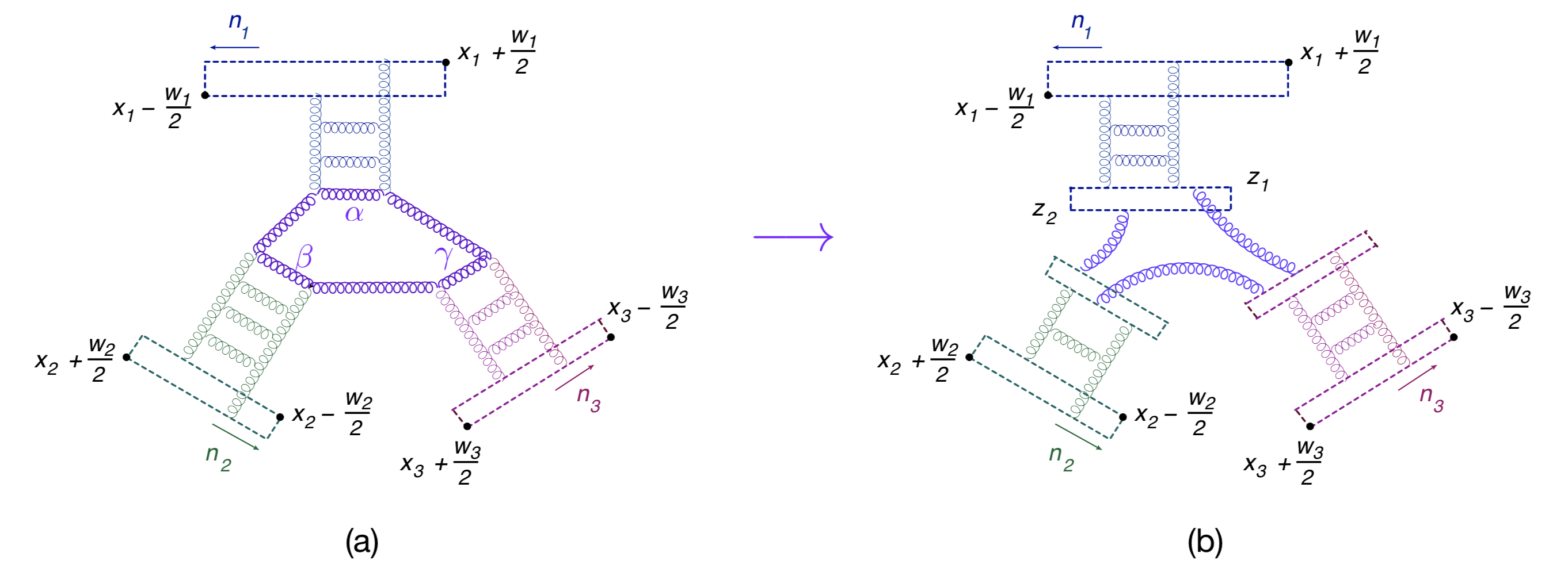
Figure 7: Triple BFKL evolution.

It is convenient to relate “triple Sudakov” variables (69) to usual Sudakov variables

$$k=\tilde{\alpha}n_{1}+\tilde{\beta}{\tilde{n}}_{1}+k_{\perp}$$ (70)

where we chose the second light-like vector as

$${\tilde{n}}_{1}~{}={s_{13}\over 2s_{23}}n_{2}+{s_{12}\over 2s_{23}}n_{3}-{n_{1}\over 4}$$ (71)

so that $-2n_{1}\cdot{\tilde{n}}_{1}\equiv{\tilde{s}}={s_{12}s_{13}\over s_{23}}$. We can rewrite Eq. (70) as follows

$$k~{}=~{}\tilde{\alpha}n_{1}+\tilde{\beta}{\tilde{n}}_{2}+{\tilde{k}}{\tilde{e}}+k_{t}e_{t}$$ (72)

where

$${\tilde{e}}~{}\equiv~{}\Big{(}n_{2}\sqrt{s_{13}\over s_{12}s_{23}}-n_{3}\sqrt{s_{12}\over s_{13}s_{23}}\Big{)},~{}~{}~{}~{}~{}~{}~{}~{}~{}~{}~{}{\tilde{e}}^{2}=1$$ (73)

The relation between variables (69) and (70) is

$$\tilde{\alpha}~{}=~{}\alpha+{\tilde{\beta}\over 4},~{}~{}~{}~{}\tilde{\beta}~{}=~{}\beta{s_{23}\over s_{13}}+\gamma{s_{23}\over s_{12}},~{}~{}~{}~{}{\tilde{k}}={1\over 2}\sqrt{s_{23}\over s_{12}s_{13}}(\beta s_{12}-\gamma s_{13})$$ (74)

As we will demonstrate below, characteristic ${\tilde{k}}$ are of order of $m_{\perp}$ (see Eq. (98)) so we can define

$$k_{\perp}^{2}~{}\equiv~{}k_{t}^{2}+{\tilde{k}}^{2}~{}\sim~{}m_{\perp}^{2}$$ (75)

In terms of these variables

$$k^{2}~{}=~{}k_{\perp}^{2}-\tilde{\alpha}\tilde{\beta}{\tilde{s}}$$ (76)

and the evolution of the $n_{1}$-parallel Wilson lines looks like the evolution considered in Sect. 5.2 for the two-point correlator of Wilson frames. Thus, we can recycle the result (55)

$${\cal F}_{n_{1}}\big{(}l_{1};x_{1t}+{w_{1t}\over 2},x_{1t}-{w_{1t}\over 2}\big{)}~{}$$ (77)

$$=~{}{iN_{c}^{2}\over\pi^{3}l_{1}}\int\!d\nu_{1}~{}\nu_{1}{2^{-4i\nu_{1}}\Gamma\big{(}{3\over 2}+i\nu_{1}\big{)}\Gamma(1-i\nu_{1})\over\Gamma\big{(}{3\over 2}-i\nu_{1}\big{)}\Gamma(1+i\nu_{1})}(w_{1t}^{2})^{-{1\over 2}+i\nu_{1}}e^{(Y_{1}-Y^{\prime}_{1})\aleph(\nu_{1})}{\cal U}^{Y^{\prime}_{1}}_{\rm conf}(x_{1t},-\nu_{1})$$

where in the LLA $Y_{1}={1\over 2}\ln{l_{1}^{2}{\tilde{s}}\over w_{1t}^{2}}\simeq\ln l_{1}+{1\over 2}\ln{\tilde{s}}m_{\perp}^{2}$ and $Y^{\prime}_{1}$ is the rapidity (${1\over 2}\ln{\tilde{\alpha}\over\tilde{\beta}}$) at which we stop the evolution.

To strengthen these coordinate-space arguments in favor of BFKL evolution in the triple Regge limit, it is shown in the Appendix 8.1 that the standard momentum-space calculation of one-loop diagrams in the triple Regge limit reproduces the first rung of the BFKL ladder for color dipoles.

It should be noted that the arguments in favor of BFKL evolution in the triple Regge limit presented above are somewhat general, so in the Appendix 8.1 I confirm them by a standard momentum-space calculation of one-loop diagrams in the triple Regge limit which reproduces the first rung of the BFKL ladder for color dipoles.

The explicit form of the conformal dipole (34) in the coordinates $z_{t}$ and ${\tilde{z}}$ reads

$${\cal U}_{\rm conf}^{a}(\nu_{1},x_{1t})~{}\equiv~{}{1\over\pi^{2}}\!\int\!{dz_{1t}d{\tilde{z}}_{1}dz_{2t}d{\tilde{z}}_{2}\over(z_{12t}^{2}+{\tilde{z}}_{12}^{2})^{2}}~{}$$ (78)

$$\times~{}\Big{(}{z_{12t}^{2}+{\tilde{z}}_{12}^{2}\over[(x_{1}-z_{1})_{t}^{2}+{\tilde{z}}_{1}^{2}][(x_{1}-z_{2})_{t}^{2}+{\tilde{z}}_{2}^{2}]}\Big{)}^{{1\over 2}-i\nu_{1}}~{}{\cal U}^{a}(z_{1t}e_{t}+{\tilde{z}}_{1}{\tilde{e}},z_{2t}e_{t}+{\tilde{z}}_{2}{\tilde{e}})$$

Repeating the same procedure for the frame parallel to $n_{2}$ we get

$${\cal F}_{n_{2}}\big{(}l_{2};x_{2t}+{w_{2t}\over 2},x_{2t}-{w_{2t}\over 2}\big{)}~{}$$ (79)

$$=~{}{iN_{c}^{2}\over\pi^{3}l_{2}}\int\!d\nu_{2}~{}\nu_{2}{2^{-4i\nu_{2}}\Gamma\big{(}{3\over 2}+i\nu_{2}\big{)}\Gamma(1-i\nu_{2})\over\Gamma\big{(}{3\over 2}-i\nu_{2}\big{)}\Gamma(1+i\nu_{2})}(w_{2t}^{2})^{-{1\over 2}+i\nu_{2}}e^{(Y_{2}-Y^{\prime}_{2})\aleph(\nu_{2})}{\cal V}^{Y^{\prime}_{2}}_{\rm conf}(x_{2t},-\nu_{2})$$

Here $Y_{2}\simeq\ln l_{2}+{1\over 2}\ln\breve{s}m_{\perp}^{2}$, $Y^{\prime}_{2}$ is the rapidity at which we stop the evolution and

$${\cal V}_{\rm conf}^{a}(\nu_{2},x_{2t})~{}\equiv~{}{1\over\pi^{2}}\!\int\!{dz_{3t}d\breve{z}_{3}dz_{4t}d\breve{z}_{4}\over(z_{34t}^{2}+\breve{z}_{34}^{2})^{2}}~{}$$ (80)

$$\times~{}\Big{(}{z_{34t}^{2}+\breve{z}_{34}^{2}\over[(x_{2}-z_{3})_{t}^{2}+\breve{z}_{3}^{2}][(x_{2}-z_{4})_{t}^{2}+\breve{z}_{4}^{2}]}\Big{)}^{{1\over 2}-i\nu_{2}}~{}{\cal V}^{a}(z_{3t}e_{t}+\breve{z}_{3},z_{4t}e_{t}+\breve{z}_{4})$$

where ${\cal V}$ is the conformal dipole with Wilson lines parallel to $n_{2}$ and

$$\breve{e}~{}\equiv~{}\Big{(}n_{3}\sqrt{s_{12}\over s_{13}s_{23}}-n_{1}\sqrt{s_{23}\over s_{12}s_{13}}\Big{)},~{}~{}~{}~{}~{}\breve{s}\equiv{s_{12}s_{23}\over s_{13}}$$ (81)

Note that the transverse plane $e_{t},\breve{e}$ for the evolution of second frame is different from the transverse plane $e_{t},{\tilde{e}}$ for the first frame.

Similarly one can get the result for the evolution of the third frame in the form

$${\cal F}_{n_{3}}\big{(}l_{3};x_{3t}+{w_{3t}\over 2},x_{3t}-{w_{3t}\over 2}\big{)}~{}$$ (82)

$$=~{}{iN_{c}^{2}\over\pi^{3}l_{3}}\int\!d\nu_{3}~{}\nu_{3}{2^{-4i\nu_{3}}\Gamma\big{(}{3\over 2}+i\nu_{3}\big{)}\Gamma(1-i\nu_{3})\over\Gamma\big{(}{3\over 2}-i\nu_{3}\big{)}\Gamma(1+i\nu_{3})}(w_{3t}^{2})^{-{1\over 2}+i\nu_{3}}e^{(Y_{3}-Y^{\prime}_{3})\aleph(\nu_{3})}{\cal W}^{Y^{\prime}_{3}}_{\rm conf}(x_{3t},-\nu_{3})$$

Here $Y_{3}\simeq\ln l_{3}+{1\over 2}\ln{\check{s}}m_{\perp}^{2}$, $Y^{\prime}_{3}$ is the rapidity at which we stop the evolution and

$${\cal W}_{\rm conf}^{a}(\nu_{3},x_{3t})~{}\equiv~{}{1\over\pi^{2}}\!\int\!{dz_{5t}d{\check{z}}_{5}dz_{6t}d{\check{z}}_{6}\over(z_{56t}^{2}+{\check{z}}_{56}^{2})^{2}}~{}$$ (83)

$$\times~{}\Big{(}{z_{56t}^{2}+{\check{z}}_{56}^{2}\over[(x_{3}-z_{5})_{t}^{2}+{\check{z}}_{5}^{2}][(x_{4}-z_{6})_{t}^{2}+{\check{z}}_{6}^{2}]}\Big{)}^{{1\over 2}-i\nu_{3}}~{}{\cal W}^{a}(z_{5t}e_{t}+{\check{z}}_{5},z_{6t}e_{t}+{\check{z}}_{6})$$

where ${\cal W}$ is the conformal dipole with Wilson lines parallel to $n_{3}$ and

$${\check{e}}~{}\equiv~{}\Big{(}n_{1}\sqrt{s_{23}\over s_{12}s_{13}}-n_{2}\sqrt{s_{13}\over s_{12}s_{23}}\Big{)},~{}~{}~{}~{}~{}{\check{s}}\equiv{s_{12}s_{23}\over s_{13}}$$ (84)

After three evolutions (77), (79), and (82) we get the correlator of three dipoles

$$\langle{\cal U}^{a}(z_{1t}e_{t}+{\tilde{z}}_{1}{\tilde{e}},z_{2t}e_{t}+{\tilde{z}}_{2}{\tilde{e}}){\cal V}^{a}(z_{3t}e_{t}+\breve{z}_{3}\breve{e},z_{4t}e_{t}+\breve{z}_{4}\breve{e})\hat{\cal W}^{a}(z_{5t}e_{t}+{\check{z}}_{5}{\check{e}},z_{6t}e_{t}+{\check{z}}_{6}{\check{e}})\rangle$$ (85)

with Wilson lines parallel to $n_{1},n_{2},n_{3}$ and rapidity cutoffs $Y^{\prime}_{1},Y^{\prime}_{2},Y^{\prime}_{3}$. Moreover, one can think about color dipoles ${\cal U}^{Y^{\prime}_{1}}$, ${\cal V}^{Y^{\prime}_{2}}$, and ${\cal W}^{Y^{\prime}_{3}}$ as long Wilson frames with lengths $l^{\prime}_{1}=e^{Y^{\prime}_{i}}\sqrt{m_{\perp}^{2}{\tilde{s}}}$ etc., see Fig. 7b. We start the evolution with very long frames and evolve with lengths of these frames.

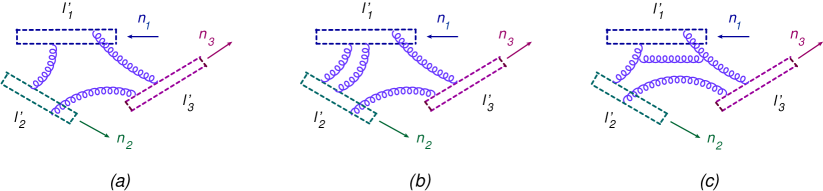
Figure 8: Three Wilson frames in the leading order (“a”) and at the one-loop level (“b”+“c”+permutations).

We should stop the evolution if an extra loop in diagrams in Fig. 8b and Fig. 8c does not bring an additional BFKL logarithm in comparison to the tree diagram in Fig. 8a. This happens when the relative energy of each pair of dipoles becomes compatible with $m_{\perp}$, or, in the coordinate space language, when the characteristic longitudinal distances are of the same order as the transverse ones so the BFKL approximations break down. For typical diagrams like in Fig. 8b or c the characteristic longitudinal separations are $\sim l^{\prime}_{i}l^{\prime}_{j}s_{ij}$ so the condition is $\sim l^{\prime}_{i}l^{\prime}_{j}\geq{1\over m_{\perp}^{2}s_{ij}}$. Thus, the three BFKL evolutions in diagrams in Fig. 7b terminate at the rapidities

$$l^{\prime}_{1}l^{\prime}_{2}\geq{1\over m_{\perp}^{2}s_{12}}~{}~{}\Leftrightarrow~{}~{}\ln l^{\prime}_{1}+\ln l^{\prime}_{2}\geq-\ln{m_{\perp}^{2}s_{12}}~{}~{}\Leftrightarrow~{}~{}Y^{\prime}_{1}+Y^{\prime}_{2}\geq 0$$

$$l^{\prime}_{1}l^{\prime}_{3}\geq{1\over m_{\perp}^{2}s_{13}}~{}~{}\Leftrightarrow~{}~{}\ln l^{\prime}_{1}+\ln l^{\prime}_{3}\geq-\ln{m_{\perp}^{2}s_{13}}~{}~{}\Leftrightarrow~{}~{}Y^{\prime}_{1}+Y^{\prime}_{3}\geq 0$$

$$l^{\prime}_{2}l^{\prime}_{3}\geq{1\over m_{\perp}^{2}s_{23}}~{}~{}\Leftrightarrow~{}~{}\ln l^{\prime}_{2}+\ln l^{\prime}_{3}\geq-\ln{m_{\perp}^{2}s_{23}}~{}~{}\Leftrightarrow~{}~{}Y^{\prime}_{2}+Y^{\prime}_{3}\geq 0$$ (86)

where $Y^{\prime}_{1}=\ln l^{\prime}_{1}+{1\over 2}\ln{\tilde{s}}m_{\perp}^{2}$, $Y^{\prime}_{2}=\ln l^{\prime}_{2}+{1\over 2}\ln\breve{s}m_{\perp}^{2}$, and $Y^{\prime}_{3}=\ln l^{\prime}_{3}+{1\over 2}\ln{\check{s}}m_{\perp}^{2}$. We see that the rapidity at which we stop the evolution of the $n_{1}$ dipole depends on the where we have terminated the evolutions of the second and third dipole which means that we need to integrate over all possible choices of “rapidity stops” $Y^{\prime}_{i}$:

$$\langle{\cal U}^{Y_{1}}_{\rm conf}(x_{1t},-\nu_{1}){\cal V}^{Y_{2}}_{\rm conf}(x_{2t},-\nu_{2}){\cal W}^{Y_{3}}_{\rm conf}(x_{3t},-\nu_{3})\rangle^{\rm Fig.\ref{fig:3bfklzlo}}$$ (87)

$$=~{}{1\over 4}\aleph(\nu_{1})\aleph(\nu_{2})\aleph(\nu_{3})\!\int_{-\infty}^{Y_{1}}\!dY^{\prime}_{1}\!\int_{-\infty}^{Y_{2}}\!dY^{\prime}_{2}\!\int_{-\infty}^{Y_{3}}\!dY^{\prime}_{3}~{}\theta\big{(}Y^{\prime}_{1}+Y^{\prime}_{2}\big{)}\theta\big{(}Y^{\prime}_{1}+Y^{\prime}_{3}\big{)}\theta\big{(}Y^{\prime}_{2}+Y^{\prime}_{3}\big{)}$$

$$\times~{}e^{(Y_{1}-Y^{\prime}_{1})\aleph(\nu_{3})}e^{(Y_{2}-Y^{\prime}_{2})\aleph(\nu_{3})}e^{(Y_{3}-Y^{\prime}_{3})\aleph(\nu_{3})}\langle{\cal U}_{\rm conf}(x_{1t},-\nu_{1}){\cal V}_{\rm conf}(x_{2t},-\nu_{2}){\cal W}_{\rm conf}(x_{3t},-\nu_{3})\rangle^{\rm tree}$$

The weight of the integrations can be figured out from the evolution equations for conformal dipoles up to an overall constant which will be determined later to be ${1\over 4}$. The factors $\aleph(\nu_{1})\aleph(\nu_{2})\aleph(\nu_{3})$ can be understood by considering the lowest-order diagram with three BFKL evolutions shown in Fig. 9.

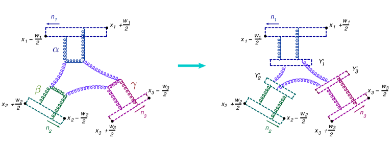
Figure 9: Three BFKL loops

The three integrations over $\alpha$, $\beta$, and $\gamma$ in Fig. 9 for conformal dipoles bring $\aleph(\nu_{i})\!\int\!dY_{i}$ for each of them so we get

$$\langle{\cal U}^{Y_{1}}_{\rm conf}(x_{1t},-\nu_{1}){\cal V}^{Y_{2}}_{\rm conf}(x_{2t},-\nu_{2}){\cal W}^{Y_{3}}_{\rm conf}(x_{3t},-\nu_{3})\rangle$$ (88)

$$\sim~{}\aleph(\nu_{1})\aleph(\nu_{2})\aleph(\nu_{3})\!\int_{-\infty}^{Y_{1}}\!dY^{\prime}_{1}\!\int_{-\infty}^{Y_{2}}\!dY^{\prime}_{2}\!\int_{-\infty}^{Y_{3}}\!dY^{\prime}_{3}~{}\theta\big{(}Y^{\prime}_{1}+Y^{\prime}_{2}\big{)}\theta\big{(}Y^{\prime}_{1}+Y^{\prime}_{3}\big{)}\theta\big{(}Y^{\prime}_{2}+Y^{\prime}_{3}\big{)}$$

$$\times~{}\langle{\cal U}_{\rm conf}(x_{1t},-\nu_{1}){\cal V}_{\rm conf}(x_{2t},-\nu_{2}){\cal W}_{\rm conf}(x_{3t},-\nu_{3})\rangle^{\rm tree}$$

Combining the equations (77), (79), (82) and Eq. (87) we get

$$\big{\langle}{\cal F}^{j_{1}}_{n_{1}}\big{(}x_{1t}+{w_{1t}\over 2},x_{1t}-{w_{1t}\over 2}\big{)}{\cal F}^{j_{2}}_{n_{2}}\big{(}x_{2t}+{w_{2t}\over 2},x_{2t}-{w_{2t}\over 2}\big{)}{\cal F}^{j_{3}}_{n_{3}}\big{(}x_{3t}+{w_{3t}\over 2},x_{3t}-{w_{3t}\over 2}\big{)}\big{\rangle}$$

$$=~{}-i{N_{c}^{6}\over\pi^{9}}\!\int_{0}^{\infty}\!\prod_{n=1}^{3}\!{dl_{n}\over l_{n}}~{}l_{n}^{-\omega_{n}}\int\!\prod_{k=1}^{3}d\nu_{k}~{}{\nu_{k}2^{-4i\nu_{k}}\Gamma\big{(}{3\over 2}+i\nu_{k}\big{)}\Gamma(1-i\nu_{k})\over\Gamma\big{(}{3\over 2}-i\nu_{k}\big{)}\Gamma(1+i\nu_{k})}(w_{kt}^{2})^{-{1\over 2}+i\nu_{k}}$$

$$\times~{}{1\over 4}\aleph(\nu_{1})\aleph(\nu_{2})\aleph(\nu_{3})\!\int_{-\infty}^{Y_{1}}\!dY^{\prime}_{1}\!\int_{-\infty}^{Y_{2}}\!dY^{\prime}_{2}\!\int_{-\infty}^{Y_{3}}\!dY^{\prime}_{3}~{}\theta\big{(}Y^{\prime}_{1}+Y^{\prime}_{2}\big{)}\theta\big{(}Y^{\prime}_{1}+Y^{\prime}_{3}\big{)}\theta\big{(}Y^{\prime}_{2}+Y^{\prime}_{3}\big{)}$$

$$\times~{}e^{(Y_{1}-Y^{\prime}_{1})\aleph(\nu_{1})}e^{(Y_{2}-Y^{\prime}_{2})\aleph(\nu_{3})}e^{(Y_{3}-Y^{\prime}_{3})\aleph(\nu_{3})}\langle{\cal U}_{\rm conf}(x_{1t},-\nu_{1}){\cal V}_{\rm conf}(x_{2t},-\nu_{2}){\cal W}_{\rm conf}(x_{3t},-\nu_{3})\rangle^{\rm tree}$$

(89)

This result is the integral over $\nu_{1},\nu_{2}$, and $\nu_{3}$ of the product of longitudinal and transverse integrals which we will consider in turn.

6.2 Longitudinal integrals

Let us integrate the correlator (89) over over $l_{i}$ according to the definition ( 25) of the “frame with spin j”. Since

$$\int_{0}^{\infty}l_{1}^{-\omega_{1}-1}~{}=~{}\int_{-\infty}^{\infty}\!dY_{1}~{}e^{-\omega_{1}Y_{1}}({\tilde{s}}m_{\perp}^{2})^{\omega_{1}\over 2}$$

(and similarly for $Y_{2}$ and $Y_{3}$) we get

$$\int_{-\infty}^{\infty}\!dY_{1}dY_{2}dY_{3}~{}e^{-\omega_{1}Y_{1}-\omega_{2}Y_{2}-\omega_{3}Y_{3}}({\tilde{s}}m_{\perp}^{2})^{\omega_{1}\over 2}(\breve{s}m_{\perp}^{2})^{\omega_{2}\over 2}({\check{s}}m_{\perp}^{2})^{\omega_{3}\over 2}$$ (90)

$$\times~{}\!\int_{-\infty}^{Y_{1}}\!dY^{\prime}_{1}\!\int_{-\infty}^{Y_{2}}\!dY^{\prime}_{2}\!\int_{-\infty}^{Y_{3}}\!dY^{\prime}_{3}~{}\theta\big{(}Y^{\prime}_{1}+Y^{\prime}_{2}\big{)}\theta\big{(}Y^{\prime}_{1}+Y^{\prime}_{3}\big{)}\theta\big{(}Y^{\prime}_{2}+Y^{\prime}_{3}\big{)}$$

$$\times~{}e^{(Y_{1}-Y^{\prime}_{1})\aleph(\nu_{1})}e^{(Y_{2}-Y^{\prime}_{2})\aleph(\nu_{3})}e^{(Y_{3}-Y^{\prime}_{3})\aleph(\nu_{3})}$$

$$=~{}{4s_{12}^{\omega_{1}+\omega_{2}-\omega_{3}\over 2}s_{13}^{\omega_{1}+\omega_{3}-\omega_{2}\over 2}s_{23}^{\omega_{2}+\omega_{3}-\omega_{1}\over 2}m_{\perp}^{-\omega_{1}-\omega_{2}-\omega_{3}}\over(\omega_{1}+\omega_{2}-\omega_{3})(\omega_{1}+\omega_{3}-\omega_{2})(\omega_{2}+\omega_{3}-\omega_{1})[\omega_{1}-\aleph(\nu_{1})][\omega_{2}-\aleph(\nu_{2})][\omega_{3}-\aleph(\nu_{3})]}$$

$$\rightarrow~{}{4\big{(}{s_{12}\over x_{12t}^{2}}\big{)}^{\omega_{1}+\omega_{2}-\omega_{3}\over 2}\big{(}{s_{13}\over x_{13t}^{2}}\big{)}^{\omega_{1}+\omega_{3}-\omega_{2}\over 2}\big{(}{s_{23}\over x_{23t}^{2}}\big{)}^{\omega_{2}+\omega_{3}-\omega_{1}\over 2}\over(\omega_{1}+\omega_{2}-\omega_{3})(\omega_{1}+\omega_{3}-\omega_{2})(\omega_{2}+\omega_{3}-\omega_{1})[\omega_{1}-\aleph(\nu_{1})][\omega_{2}-\aleph(\nu_{2})][\omega_{3}-\aleph(\nu_{3})]}$$

We have replaced the transverse scale $m_{\perp}^{-2}$ by $x_{ijt}^{2}$ in accordance with general formula (19) and the result (138) of explicit first-order calculation performed in Appendix 8.2.

Also, as discussed in Ref. Balitsky:2015oux , the singularities $(\omega_{i}-\omega_{j}-\omega_{k})^{-1}$ are of general nature since they arise from the fact that the correlator of three Wilson frames (27) acquires boost invariance as $n_{j}\rightarrow n_{k}$. This property is discussed in Appendix 8.3.

6.3 Transverse integral

Using Eq. (90) of previous Section, one can rewrite the result (89) as

$$\big{\langle}{\cal F}^{j_{1}}_{n_{1}}\big{(}x_{1t}+{w_{1t}\over 2},x_{1t}-{w_{1t}\over 2}\big{)}{\cal F}^{j_{2}}_{n_{2}}\big{(}x_{2t}+{w_{2t}\over 2},x_{2t}-{w_{2t}\over 2}\big{)}{\cal F}^{j_{3}}_{n_{3}}\big{(}x_{3t}+{w_{3t}\over 2},x_{3t}-{w_{3t}\over 2}\big{)}\big{\rangle}$$

$$=~{}-i{N_{c}^{6}\over\pi^{9}}\int\!d\nu_{1}d\nu_{2}d\nu_{3}~{}\prod_{k=1}^{3}{\nu_{k}2^{-4i\nu_{k}}\Gamma\big{(}{3\over 2}+i\nu_{k}\big{)}\Gamma(1-i\nu_{k})\over\Gamma\big{(}{3\over 2}-i\nu_{k}\big{)}\Gamma(1+i\nu_{k})}(w_{kt}^{2})^{-{1\over 2}+i\nu_{k}}$$

$$\times~{}{\aleph(\nu_{1})\aleph(\nu_{2})\aleph(\nu_{3})\big{(}{s_{12}\over x_{12t}^{2}}\big{)}^{\omega_{1}+\omega_{2}-\omega_{3}\over 2}\big{(}{s_{13}\over x_{13t}^{2}}\big{)}^{\omega_{1}+\omega_{3}-\omega_{2}\over 2}\big{(}{s_{23}\over x_{23t}^{2}}\big{)}^{\omega_{2}+\omega_{3}-\omega_{1}\over 2}\over(\omega_{1}+\omega_{2}-\omega_{3})(\omega_{1}+\omega_{3}-\omega_{2})(\omega_{2}+\omega_{3}-\omega_{1})[\omega_{1}-\aleph(\nu_{1})][\omega_{2}-\aleph(\nu_{2})][\omega_{3}-\aleph(\nu_{3})]}$$

$$\times~{}\langle{\cal U}^{Y^{\prime}_{1}}_{\rm conf}(x_{1t},-\nu_{1}){\cal V}^{Y^{\prime}_{2}}_{\rm conf}(x_{2t},-\nu_{2}){\cal W}^{Y^{\prime}_{3}}_{\rm conf}(x_{3t},-\nu_{3})\rangle^{\rm tree}$$ (91)

where the correlator of three conformal dipoles in the last line should be taken in the tree approximation.

To calculate this correlator, we rewrite conformal dipoles in terms of usual ones

$$\pi^{6}\langle{\cal U}^{Y^{\prime}_{1}}_{\rm conf}(x_{1t},-\nu_{1}){\cal V}^{Y^{\prime}_{2}}_{\rm conf}(x_{2t},-\nu_{2}){\cal W}^{Y^{\prime}_{3}}_{\rm conf}(x_{3t},-\nu_{3})\rangle^{\rm tree}~{}=~{}\int\!{dz_{1t}d{\tilde{z}}_{1}dz_{2t}d{\tilde{z}}_{2}\over(z_{12t}^{2}+{\tilde{z}}_{12}^{2})^{2}}$$ (92)

$$\times~{}\int\!{dz_{3t}d\breve{z}_{3}dz_{4t}d\breve{z}_{4}\over(z_{34t}^{2}+\breve{z}_{34}^{2})^{2}}{dz_{5t}d{\check{z}}_{5}dz_{6t}d{\check{z}}_{6}\over(z_{56t}^{2}+{\check{z}}_{56}^{2})^{2}}\Big{(}{z_{12t}^{2}+{\tilde{z}}_{12}^{2}\over[(x_{1}-z_{1})_{t}^{2}+{\tilde{z}}_{1}^{2}][(x_{1}-z_{2})_{t}^{2}+{\tilde{z}}_{2}^{2}]}\Big{)}^{{1\over 2}+i\nu_{1}}$$

$$\times~{}\Big{(}{z_{34t}^{2}+\breve{z}_{34}^{2}\over[(x_{2}-z_{3})_{t}^{2}+\breve{z}_{3}^{2}][(x_{2}-z_{4})_{t}^{2}+\breve{z}_{4}^{2}]}\Big{)}^{{1\over 2}+i\nu_{2}}\Big{(}{z_{56t}^{2}+{\check{z}}_{56}^{2}\over[(x_{3}-z_{5})_{t}^{2}+{\check{z}}_{5}^{2}][(x_{3}-z_{6})_{t}^{2}+{\check{z}}_{6}^{2}]}\Big{)}^{{1\over 2}+i\nu_{3}}~{}$$

$$\times~{}\langle{\cal U}(z_{1t}e_{t}+{\tilde{z}}_{1}{\tilde{e}},z_{2t}e_{t}+{\tilde{z}}_{2}{\tilde{e}}){\cal V}(z_{3t}e_{t}+\breve{z}_{3}\breve{e},z_{4t}e_{t}+\breve{z}_{4}\breve{e})\hat{\cal W}(z_{5t}e_{t}+{\check{z}}_{5}{\check{e}},z_{6t}e_{t}+{\check{z}}_{6}{\check{e}})\rangle$$

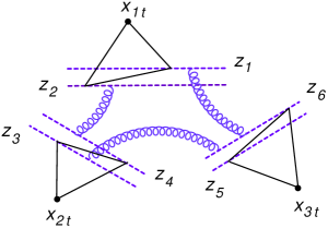
Figure 10: The structure of correlator (92). Straight lines denote “propagators” $(z_{ij}^{2})^{\lambda}$ or $((x_{i}-z_{j})^{2})^{\lambda}$.

This integral is illustrated on Fig. 10.

Using the leading-order correlator

$$\langle[\infty n_{1}+x,-\infty n_{1}+x][\infty n_{2}+y,-\infty n_{2}+y]\rangle~{}=~{}i\alpha_{s}t^{a}\otimes t^{a}\ln\Big{[}(x-y)^{2}-2{(x-y)_{n_{1}}(x-y)_{n_{2}}\over n_{1}\cdot n_{2}}\Big{]}$$ (93)

one easily obtains

$$\langle{U}(z_{1t}e_{t}+{\tilde{z}}_{1}{\tilde{e}}){V}(z_{3t}e_{t}+\breve{z}_{3}\breve{e})\rangle~{}=~{}i\alpha_{s}t^{a}\otimes t^{a}\ln[z_{13t}^{2}+({\tilde{z}}_{1}+\breve{z}_{3})^{2}],$$

$$\langle{U}(z_{1t}e_{t}+{\tilde{z}}_{1}{\tilde{e}}){W}(z_{5t}e_{t}+{\check{z}}_{5}{\check{e}})\rangle~{}=~{}i\alpha_{s}t^{a}\otimes t^{a}\ln[z_{15t}^{2}+({\tilde{z}}_{1}+{\check{z}}_{5})^{2}],$$

$$\langle{V}(z_{3t}e_{t}+\breve{z}_{3}\breve{e}){W}(z_{5t}e_{t}+{\check{z}}_{5}{\check{e}})\rangle~{}=~{}i\alpha_{s}t^{a}\otimes t^{a}\ln[z_{35t}^{2}+(\breve{z}_{3}+{\check{z}}_{5})^{2}]$$ (94)

and therefore the tree-level correlator of three color dipoles reads

$$\langle{\cal U}^{a}(z_{1t}e_{t}+{\tilde{z}}_{1}{\tilde{e}},z_{2t}e_{t}+{\tilde{z}}_{2}{\tilde{e}}){\cal V}^{a}(z_{3t}e_{t}+\breve{z}_{3}\breve{e},z_{4t}e_{t}+\breve{z}_{4}\breve{e})\hat{\cal W}^{a}(z_{5t}e_{t}+{\check{z}}_{5}{\check{e}},z_{6t}e_{t}+{\check{z}}_{6}{\check{e}})\rangle$$

$$=~{}-i\alpha_{s}^{3}{N_{c}^{2}-1\over N_{c}^{3}}\ln{[z_{13t}^{2}+({\tilde{z}}_{1}+\breve{z}_{3})^{2}][z_{24t}^{2}+({\tilde{z}}_{2}+\breve{z}_{4})^{2}]\over[z_{14t}^{2}+({\tilde{z}}_{1}+\breve{z}_{4})^{2}][z_{23t}^{2}+({\tilde{z}}_{2}+\breve{z}_{3})^{2}]}$$

$$\times~{}\ln{[z_{15t}^{2}+({\tilde{z}}_{1}+{\check{z}}_{5})^{2}][z_{26t}^{2}+({\tilde{z}}_{2}+{\check{z}}_{6})^{2}]\over[z_{16t}^{2}+({\tilde{z}}_{1}+{\check{z}}_{6})^{2}][z_{25t}^{2}+({\tilde{z}}_{2}+{\check{z}}_{5})^{2}]}\ln{[z_{35t}^{2}+(\breve{z}_{3}+{\check{z}}_{5})^{2}][z_{46t}^{2}+(\breve{z}_{4}+{\check{z}}_{6})^{2}]\over[z_{36t}^{2}+(\breve{z}_{3}+{\check{z}}_{6})^{2}][z_{45t}^{2}+(\breve{z}_{4}+{\check{z}}_{5})^{2}]}$$ (95)

One obtains

$$\langle{\cal U}_{\rm conf}(x_{1t},-\nu_{1}){\cal V}_{\rm conf}(x_{2t},-\nu_{2}){\cal W}_{\rm conf}(x_{3t},-\nu_{3})\rangle^{\rm tree}~{}$$

$$\hskip 31.29802pt=~{}-i\alpha_{s}^{3}{N_{c}^{2}-1\over N_{c}^{3}\pi^{6}}I(x_{1t},x_{2t},x_{3t};\nu_{1},\nu_{2},\nu_{3})$$

(96)

where

$$I(x_{1t},x_{2t},x_{3t};\nu_{1},\nu_{2},\nu_{3})~{}=~{}\!\int\!{dz_{1t}d{\tilde{z}}_{1}dz_{2t}d{\tilde{z}}_{2}\over(z_{12t}^{2}+{\tilde{z}}_{12}^{2})^{2}}{dz_{3t}d\breve{z}_{3}dz_{4t}d\breve{z}_{4}\over(z_{34t}^{2}+\breve{z}_{34}^{2})^{2}}{dz_{5t}d{\check{z}}_{5}dz_{6t}d{\check{z}}_{6}\over(z_{56t}^{2}+{\check{z}}_{56}^{2})^{2}}$$

$$\times~{}\Big{(}{z_{12t}^{2}+{\tilde{z}}_{12}^{2}\over[(x_{1}-z_{1})_{t}^{2}+{\tilde{z}}_{1}^{2}][(x_{1}-z_{2})_{t}^{2}+{\tilde{z}}_{2}^{2}]}\Big{)}^{{1\over 2}+i\nu_{1}}\Big{(}{z_{34t}^{2}+\breve{z}_{34}^{2}\over[(x_{2}-z_{3})_{t}^{2}+\breve{z}_{3}^{2}][(x_{2}-z_{4})_{t}^{2}+\breve{z}_{4}^{2}]}\Big{)}^{{1\over 2}+i\nu_{2}}$$

$$\times~{}\Big{(}{z_{56t}^{2}+{\check{z}}_{56}^{2}\over[(x_{3}-z_{5})_{t}^{2}+{\check{z}}_{5}^{2}][(x_{3}-z_{6})_{t}^{2}+{\check{z}}_{6}^{2}]}\Big{)}^{{1\over 2}+i\nu_{3}}\ln{[z_{13t}^{2}+({\tilde{z}}_{1}+\breve{z}_{3})^{2}][z_{24t}^{2}+({\tilde{z}}_{2}+\breve{z}_{4})^{2}]\over[z_{14t}^{2}+({\tilde{z}}_{1}+\breve{z}_{4})^{2}][z_{23t}^{2}+({\tilde{z}}_{2}+\breve{z}_{3})^{2}]}$$

$$\times~{}\ln{[z_{15t}^{2}+({\tilde{z}}_{1}+{\check{z}}_{5})^{2}][z_{26t}^{2}+({\tilde{z}}_{2}+{\check{z}}_{6})^{2}]\over[z_{16t}^{2}+({\tilde{z}}_{1}+{\check{z}}_{6})^{2}][z_{25t}^{2}+({\tilde{z}}_{2}+{\check{z}}_{5})^{2}]}\ln{[z_{35t}^{2}+(\breve{z}_{3}+{\check{z}}_{5})^{2}][z_{46t}^{2}+(\breve{z}_{4}+{\check{z}}_{6})^{2}]\over[z_{36t}^{2}+(\breve{z}_{3}+{\check{z}}_{6})^{2}][z_{45t}^{2}+(\breve{z}_{4}+{\check{z}}_{5})^{2}]}$$ (97)

The structure of the integrations in this equation is the following: each conformal dipole evolves in its own “transverse plane” and the obtained dipoles interact by logarithmical correlators (94). Fortunately, the integral (97) coincides with an usual two-dimensional integral in the (formal) $(x,y)$ plane

$$I(x_{1},x_{2},x_{3};\nu_{1},\nu_{2},\nu_{3})~{}=~{}\!\int\!{d^{2}z_{1}d^{2}z_{2}\over z_{12}^{4}}{d^{2}z_{3}d^{2}z_{4}\over z_{34}^{4}}{d^{2}z_{5}d^{2}z_{6}\over z_{56}^{4}}$$

$$\times~{}\Big{(}{z_{12}^{2}\over(x_{1}-z_{1})^{2}(x_{1}-z_{2})^{2}}\Big{)}^{{1\over 2}+i\nu_{1}}\Big{(}{z_{34}^{2}\over(x_{2}-z_{3})^{2}(x_{2}-z_{4})^{2}]}\Big{)}^{{1\over 2}+i\nu_{2}}\Big{(}{z_{56}^{2}\over(x_{3}-z_{5})^{2}(x_{3}-z_{6})^{2}]}\Big{)}^{{1\over 2}+i\nu_{2}}$$

$$\times~{}\ln{[z_{13x}^{2}+(z_{1y}+z_{3y})^{2}][z_{24x}^{2}+(z_{2y}+z_{4y})^{2}]\over[z_{14x}^{2}+(z_{1y}+z_{4y})^{2}][z_{23x}^{2}+(z_{2y}+z_{3y})^{2}]}\ln{[z_{15x}^{2}+(z_{1y}+z_{5y})^{2}][z_{26x}^{2}+(z_{2y}+z_{6y})^{2}]\over[z_{16x}^{2}+(z_{1y}+z_{6y})^{2}][z_{25x}^{2}+(z_{2y}+z_{5y})^{2}]}$$

$$\times~{}\ln{[z_{35x}^{2}+(z_{3y}+z_{5y})^{2}][z_{46x}^{2}+(z_{4y}+z_{6y})^{2}]\over[z_{36x}^{2}+(z_{3y}+z_{6y})^{2}][z_{45x}^{2}+(z_{4y}+z_{5y})^{2}]}$$ (98)

with $x_{1y}=x_{2y}=x_{3y}=0$, see Fig.11a.

Figure 11: Transverse integral. Solid lines denote usual “propagators” of the type $(z_{i}-z_{j})^{2\lambda}$ and dotted lines expressions of the type $[(z_{i}-z_{j})_{x}^{2}+(z_{i}+z_{j})_{y}^{2}]^{\lambda}$.

Next, we use formula

$$\int\!{d^{2}z_{2}\over z_{12}^{4}}\Big{(}{z_{12}^{2}\over(x_{1}-z_{1})^{2}(x_{1}-z_{2})^{2}}\Big{)}^{{1\over 2}+i\nu_{1}}\ln z_{23}^{2}~{}=~{}{\pi[(x_{1}-z_{1})^{2}]^{-{3\over 2}-i\nu_{1}}\over\big{(}{1\over 2}-i\nu_{1}\big{)}^{2}}\Big{[}\Big{(}{(x_{1}-z_{3})^{2}\over z_{13}^{2}}\Big{)}^{{1\over 2}-i\nu_{1}}-1\Big{]}$$

and rewrite it by changing sign of $z_{3y}$ as

$$\int\!{d^{2}z_{2}\over z_{12}^{4}}\Big{(}{z_{12}^{2}\over(x_{1}-z_{1})^{2}(x_{1}-z_{2})^{2}}\Big{)}^{{1\over 2}+i\nu}\ln[z_{23x}^{2}+(z_{2y}+z_{3y})^{2}]$$

$$=~{}{\pi[(x_{1}-z_{1})^{2}]^{-{3\over 2}-i\nu_{1}}\over\big{(}{1\over 2}-i\nu_{1}\big{)}^{2}}\Big{[}\Big{(}{(x_{1}-z_{3})^{2}\over z_{13x}^{2}+(z_{1y}+z_{3y})^{2}}\Big{)}^{{1\over 2}-i\nu_{1}}-1\Big{]}$$ (99)

Using this integral and similar integrals for integration over $z_{4}$ and $z_{6}$ one gets after some algebra (see Fig.11b)

$$I(x_{1},x_{2},x_{3};\nu_{1},\nu_{2},\nu_{3})$$ (100)

$$=~{}-{8\pi^{3}\over\big{(}{1\over 2}-i\nu_{1}\big{)}^{2}\big{(}{1\over 2}-i\nu_{2}\big{)}^{2}\big{(}{1\over 2}-i\nu_{3}\big{)}^{2}}\!\int\!{d^{2}z_{1}\over(x_{1}-z_{1})^{4}}{d^{2}z_{3}\over(x_{2}-z_{3})^{4}}{d^{2}z_{5}\over(x_{3}-z_{5})^{4}}$$

$$\times~{}\Big{[}{z_{13x}^{2}+(z_{1y}+z_{3y})^{2}\over(x_{1}-z_{1})^{2}(x_{1}-z_{3})^{2}}\Big{]}^{-{1\over 2}+i\nu_{1}}\Big{[}{z_{35x}^{2}+(z_{3y}+z_{5y})^{2}\over(x_{2}-z_{3})^{2}(x_{2}-z_{5})^{2}}\Big{]}^{-{1\over 2}+i\nu_{2}}\Big{[}{z_{15x}^{2}+(z_{1y}+z_{5y})^{2}\over(x_{3}-z_{1})^{2}(x_{3}-z_{5})^{2}}\Big{]}^{-{1\over 2}+i\nu_{3}}$$

To calculate this integral, we can take $x_{1}=0$ and perform the inversion $x_{i}\rightarrow{x_{i}\over x^{2}}$ to obtain

$$I^{\rm inv}(x_{1},x_{2},x_{3};\nu_{1},\nu_{2},\nu_{3})$$

$$=~{}-{8\pi^{3}(x_{2}^{2})^{1+2i\nu_{2}}(x_{3}^{2})^{1+2i\nu_{3}}\over\big{(}{1\over 2}-i\nu_{1}\big{)}^{2}\big{(}{1\over 2}-i\nu_{2}\big{)}^{2}\big{(}{1\over 2}-i\nu_{3}\big{)}^{2}}\!\int\!d^{2}z_{1}{d^{2}z_{3}\over(x_{2}-z_{3})^{4}}{d^{2}z_{5}\over(x_{3}-z_{5})^{4}}$$

$$\times~{}[z_{13x}^{2}+(z_{1y}+z_{3y})^{2}]^{-{1\over 2}+i\nu_{1}}\Big{[}{z_{35x}^{2}+(z_{3y}+z_{5y})^{2}\over(x_{2}-z_{3})^{2}(x_{2}-z_{5})^{2}}\Big{]}^{-{1\over 2}+i\nu_{2}}\Big{[}{z_{15x}^{2}+(z_{1y}+z_{5y})^{2}\over(x_{3}-z_{1})^{2}(x_{3}-z_{5})^{2}}\Big{]}^{-{1\over 2}+i\nu_{3}}$$

$$=~{}-{8\pi^{6}(x_{2}^{2})^{1+2i\nu_{2}}(x_{3}^{2})^{1+2i\nu_{3}}(x_{23}^{2})^{-{1\over 2}+i(\nu_{1}-\nu_{2}-\nu_{3})}\over\big{(}{1\over 2}-i\nu_{1}\big{)}^{2}\big{(}{1\over 2}-i\nu_{2}\big{)}^{2}\big{(}{1\over 2}-i\nu_{3}\big{)}^{2}}\Lambda(\nu_{1},\nu_{2},\nu_{3})$$ (101)

where

$$\Lambda(\nu_{1},\nu_{2},\nu_{3})~{}\equiv~{}(x_{23}^{2})^{{1\over 2}-i(\nu_{1}-\nu_{2}-\nu_{3})}{1\over\pi^{3}}\!\int\!d^{2}z_{1}{d^{2}z_{3}\over(x_{23}-z_{3})^{4}}{d^{2}z_{5}\over z_{5}^{4}}$$

$$\times~{}[z_{13x}^{2}+(z_{1y}+z_{3y})^{2}]^{-{1\over 2}+i\nu_{1}}\Big{[}{z_{35}^{2}\over(x_{23}-z_{3})^{2}(x_{23}-z_{5})^{2}}\Big{]}^{-{1\over 2}+i\nu_{2}}\Big{[}{z_{15}^{2}\over z_{1}^{2}z_{5}^{2}}\Big{]}^{-{1\over 2}+i\nu_{3}}$$

$$=~{}{1\over\pi^{3}}\!\int\!d^{2}z_{1}{d^{2}z_{3}\over(1-z_{3})^{4}}{d^{2}z_{5}\over z_{5}^{4}}$$

$$\times~{}[z_{13x}^{2}+(z_{1y}+z_{3y})^{2}]^{-{1\over 2}+i\nu_{1}}\Big{[}{z_{35}^{2}\over(1-z_{3})^{2}(1-z_{5})^{2}}\Big{]}^{-{1\over 2}+i\nu_{2}}\Big{[}{z_{15}^{2}\over z_{1}^{2}z_{5}^{2}}\Big{]}^{-{1\over 2}+i\nu_{3}}$$ (102)

where “1” in the denominators stands for the vector (1,0). This integral resembles the integral for function $\Omega$ defining three-pomeron vertex Korchemsky:1997fy , only with “modified propagator” $[z_{13x}^{2}+(z_{1y}+z_{3y})^{2}]^{-{1\over 2}+i\nu_{1}}$ instead of usual $[z_{13x}^{2}+z_{13y}^{2}]^{-{1\over 2}+i\nu_{1}}$ in Ref. Korchemsky:1997fy . The function $\Lambda(\nu_{1},\nu_{2},\nu_{3})$ can be represented as four-fold Mellin-Barnes integral, see Eq. (107) below and Eq. (172) in Appendix 8.4.

Performing inversion of Eq. (101) we get

$$I(x_{1t},x_{2t},x_{3t};\nu_{1},\nu_{2},\nu_{3})~{}=~{}-8\pi^{6}{\Lambda(\nu_{1},\nu_{2},\nu_{3})\over\big{(}{1\over 2}-i\nu_{1}\big{)}^{2}\big{(}{1\over 2}-i\nu_{2}\big{)}^{2}\big{(}{1\over 2}-i\nu_{3}\big{)}^{2}}$$

$$\times~{}(x_{12t}^{2})^{-{1\over 2}-i(\nu_{1}+\nu_{2}-\nu_{3})}(x_{13t}^{2})^{-{1\over 2}-i(\nu_{1}+\nu_{3}-\nu_{2})}(x_{23t}^{2})^{-{1\over 2}-i(\nu_{2}+\nu_{3}-\nu_{1})}$$ (103)

so that

$$\langle{\cal U}_{\rm conf}(x_{1t},-\nu_{1}){\cal V}_{\rm conf}(x_{2t},-\nu_{2}){\cal W}_{\rm conf}(x_{3t},-\nu_{3})\rangle^{\rm tree}~{}$$ (104)

$$=~{}8i\alpha_{s}^{3}{N_{c}^{2}-1\over N_{c}^{3}}\Lambda(\nu_{1},\nu_{2},\nu_{3}){(x_{12t}^{2})^{-{1\over 2}-i(\nu_{1}+\nu_{2}-\nu_{3})}(x_{13t}^{2})^{-{1\over 2}-i(\nu_{1}+\nu_{3}-\nu_{2})}(x_{23t}^{2})^{-{1\over 2}-i(\nu_{2}+\nu_{3}-\nu_{1})}\over\big{(}{1\over 2}-i\nu_{1}\big{)}^{2}\big{(}{1\over 2}-i\nu_{2}\big{)}^{2}\big{(}{1\over 2}-i\nu_{3}\big{)}^{2}}$$

6.4 The result

Substituting the transverse integral (104) into Eq. (91) we get

$$\big{\langle}{\cal F}^{j_{1}}_{n_{1}}\big{(}x_{1t}+{w_{1t}\over 2},x_{1t}-{w_{1t}\over 2}\big{)}{\cal F}^{j_{2}}_{n_{2}}\big{(}x_{2t}+{w_{2t}\over 2},x_{2t}-{w_{2t}\over 2}\big{)}{\cal F}^{j_{3}}_{n_{3}}\big{(}x_{3t}+{w_{3t}\over 2},x_{3t}-{w_{3t}\over 2}\big{)}\big{\rangle}$$

$$=~{}{64g^{6}\over\pi^{6}}(N_{c}^{2}-1)\int_{-\infty}^{\infty}\!d\nu_{1}d\nu_{2}d\nu_{3}~{}\prod_{k=1}^{3}{\nu_{k}2^{-4i\nu_{k}}\Gamma\big{(}{3\over 2}+i\nu_{k}\big{)}\Gamma(1-i\nu_{k})\over\Gamma\big{(}{3\over 2}-i\nu_{k}\big{)}\Gamma(1+i\nu_{k})}(w_{kt}^{2})^{-{1\over 2}+i\nu_{k}}$$

$$\times~{}{8\aleph(\nu_{1})\aleph(\nu_{2})\aleph(\nu_{3})\big{(}{s_{12}\over x_{12t}^{2}}\big{)}^{\omega_{1}+\omega_{2}-\omega_{3}\over 2}\big{(}{s_{13}\over x_{13t}^{2}}\big{)}^{\omega_{1}+\omega_{3}-\omega_{2}\over 2}\big{(}{s_{23}\over x_{23t}^{2}}\big{)}^{\omega_{2}+\omega_{3}-\omega_{1}\over 2}\over(\omega_{1}+\omega_{2}-\omega_{3})(\omega_{1}+\omega_{3}-\omega_{2})(\omega_{2}+\omega_{3}-\omega_{1})[\omega_{1}-\aleph(\nu_{1})][\omega_{2}-\aleph(\nu_{2})][\omega_{3}-\aleph(\nu_{3})]}$$

$$\times~{}{(x_{12t}^{2})^{-{1\over 2}-i(\nu_{1}+\nu_{2}-\nu_{3})}(x_{13t}^{2})^{-{1\over 2}-i(\nu_{1}+\nu_{3}-\nu_{2})}(x_{23t}^{2})^{-{1\over 2}-i(\nu_{2}+\nu_{3}-\nu_{1})}\over\big{(}{1\over 2}-i\nu_{1}\big{)}^{2}\big{(}{1\over 2}-i\nu_{2}\big{)}^{2}\big{(}{1\over 2}-i\nu_{3}\big{)}^{2}}\Lambda(\nu_{1},\nu_{2},\nu_{3})$$ (105)

To estimate this integral at small $\omega$’s it is convenient to rewrite it in variables $\gamma_{i}=2i\nu_{i}-1$. Defining $\tilde{\aleph}(\gamma_{i})\equiv\aleph(\nu_{i})$ and $\tilde{\Lambda}(\gamma_{i})\equiv\Lambda(\nu_{i})$ we get

$$\big{\langle}{\cal F}^{j_{1}}_{n_{1}}\big{(}x_{1t}+{w_{1t}\over 2},x_{1t}-{w_{1t}\over 2}\big{)}{\cal F}^{j_{2}}_{n_{2}}\big{(}x_{2t}+{w_{2t}\over 2},x_{2t}-{w_{2t}\over 2}\big{)}{\cal F}^{j_{3}}_{n_{3}}\big{(}x_{3t}+{w_{3t}\over 2},x_{3t}-{w_{3t}\over 2}\big{)}\big{\rangle}$$

$$=~{}-{8g^{6}(N_{c}^{2}-1)\over\pi^{6}x_{12t}^{2}x_{13t}^{2}x_{23t}^{2}}{\big{(}{s_{12}\over x_{12t}^{2}}\big{)}^{\omega_{1}+\omega_{2}-\omega_{3}\over 2}\big{(}{s_{13}\over x_{13t}^{2}}\big{)}^{\omega_{1}+\omega_{3}-\omega_{2}\over 2}\big{(}{s_{23}\over x_{23t}^{2}}\big{)}^{\omega_{2}+\omega_{3}-\omega_{1}\over 2}\over(\omega_{1}+\omega_{2}-\omega_{3})(\omega_{1}+\omega_{3}-\omega_{2})(\omega_{2}+\omega_{3}-\omega_{1})}$$

$$\times~{}\int_{-1-i\infty}^{-1+i\infty}\!d\gamma_{1}d\gamma_{2}d\gamma_{3}~{}\prod_{k=1}^{3}{(1+\gamma_{k})2^{-2\gamma_{k}}\Gamma\big{(}2+{\gamma_{k}\over 2}\big{)}\Gamma\big{(}{1\over 2}-{\gamma_{k}\over 2}\big{)}\over\Gamma\big{(}1-{\gamma_{k}\over 2}\big{)}\Gamma\big{(}{3\over 2}+{\gamma_{k}\over 2}\big{)}\gamma_{k}^{2}}$$

$$\times~{}{\tilde{\aleph}(\gamma_{1})\tilde{\aleph}(\gamma_{2})\tilde{\aleph}(\gamma_{3})\tilde{\Lambda}(\gamma_{1},\gamma_{2},\gamma_{3})\over[\omega_{1}-\tilde{\aleph}(\gamma_{1})][\omega_{2}-\tilde{\aleph}(\gamma_{2})][\omega_{3}-\tilde{\aleph}(\gamma_{3})]}\Big{(}{w_{1t}^{2}x_{23t}^{2}\over x_{12t}^{2}x_{13t}^{2}}\Big{)}^{\gamma_{1}\over 2}\Big{(}{w_{2t}^{2}x_{13t}^{2}\over x_{12t}^{2}x_{23t}^{2}}\Big{)}^{\gamma_{2}\over 2}\Big{(}{w_{3t}^{2}x_{12t}^{2}\over x_{13t}^{2}x_{23t}^{2}}\Big{)}^{\gamma_{3}\over 2}$$ (106)

where contours over real $\nu_{i}$ transform to the contours parallel to imaginary axis since $\gamma_{i}=2i\nu_{i}-1$. The function $\tilde{\Lambda}(\gamma_{i})$ (defined by Eq. (102)) is represented in Appendix 8.4 as

$${\bar{\Lambda}}(\epsilon_{1},\epsilon_{2},\epsilon_{3})~{}=~{}-{\sin^{2}\pi\epsilon_{2}\sin^{2}\pi\epsilon_{3}\over\pi^{3}\sin\pi(\epsilon_{2}+\epsilon_{3})\Gamma^{2}(\epsilon_{1})}I(\epsilon_{1},\epsilon_{2},\epsilon_{3})$$ (107)

where ${\bar{\Lambda}}(\epsilon_{i})\equiv\tilde{\Lambda}(\gamma_{i})$, $\epsilon_{i}\equiv-{\gamma_{i}\over 2}$ and

$$I(\epsilon_{1},\epsilon_{2},\epsilon_{3})~{}$$ (108)

$$=~{}\!\int_{C}\!{ds_{1}ds_{2}ds_{3}ds_{4}\over(2\pi i)^{4}}~{}\Gamma(\epsilon_{1}-s_{1}-s_{2})\Gamma(s_{1})\Gamma(s_{2})\Gamma(\epsilon_{1}-s_{3}-s_{4})\Gamma(s_{3})\Gamma(s_{4})$$

$$\times~{}{\Gamma(\epsilon_{2}-1-s_{1})\Gamma(s_{1}+1)\over\Gamma(\epsilon_{2})}~{}{\Gamma(1+\epsilon_{3}-s_{3})\Gamma(-1+s_{3})\over\Gamma(\epsilon_{3})}~{}$$

$$\times~{}{\Gamma(\epsilon_{2}-1-s_{4})\Gamma(1-\epsilon_{1}-\epsilon_{2}+s_{3}+s_{4})\over\Gamma(-\epsilon_{1}+s_{3})}$$

$$\times~{}{\Gamma(1+\epsilon_{3}-s_{2})\Gamma(1-\epsilon_{1}-\epsilon_{3}+s_{1}+s_{2})\over\Gamma(2-\epsilon_{1}+s_{1})}{\Gamma(\epsilon_{2}-s_{1})\Gamma(\epsilon_{3}-s_{3})\over\Gamma(\epsilon_{2}+\epsilon_{3}-s_{1}-s_{3})}{\Gamma(\epsilon_{2}-s_{2})\Gamma(\epsilon_{3}-s_{4})\over\Gamma(\epsilon_{2}+\epsilon_{3}-s_{2}-s_{4})}$$

is a four-fold Mellin-Barnes integral with the contour C specified in the Appendix.

In the limit $w_{it}^{2}\rightarrow 0$ the contours of integration over $\gamma_{i}$ can be moved to the right so the integrals are determined by the residues lying on the real axis to the right of point $\gamma_{i}=-1$. As demonstrated in Appendix 8.4, the function $\Lambda$ is regular at small $\gamma_{i}$

$$\tilde{\Lambda}(\gamma_{i})~{}=~{}1+O(\gamma_{i})$$ (109)

so the analytic structure of the integral (106) is determined by the poles in $\Gamma$-functions and in $[\omega-\aleph(\gamma)]^{-1}$ denominators. The leftmost of such poles are located at $\gamma_{i}=0$ and at $\gamma_{i}^{\ast}(\omega_{i},g^{2})$ = roots of equation (21) which simplifies to

$$\omega_{i}~{}=~{}\tilde{\aleph}(\gamma_{i},g^{2})~{}=~{}4g^{2}\big{[}2\psi(1)-\psi\big{(}-{\gamma_{i}\over 2}\big{)}-\psi\big{(}1+{\gamma_{i}\over 2}\big{)}\big{]}$$ (110)

in the leading log approximation, see the discussion in Sect. 3.2.

First, we consider poles at $\gamma_{i}^{\ast}(\omega_{i},g^{2})$. Taking residues in these poles we obtain

$$\big{\langle}{\cal F}^{j_{1}}_{n_{1}}\big{(}x_{1t}+{w_{1t}\over 2},x_{1t}-{w_{1t}\over 2}\big{)}{\cal F}^{j_{2}}_{n_{2}}\big{(}x_{2t}+{w_{2t}\over 2},x_{2t}-{w_{2t}\over 2}\big{)}{\cal F}^{j_{3}}_{n_{3}}\big{(}x_{3t}+{w_{3t}\over 2},x_{3t}-{w_{3t}\over 2}\big{)}\big{\rangle}$$

$$=~{}i{64g^{6}(N_{c}^{2}-1)\over\pi^{3}x_{12t}^{2}x_{13t}^{2}x_{23t}^{2}}{\omega_{1}\omega_{2}\omega_{3}\big{(}{s_{12}\over x_{12t}^{2}}\big{)}^{\omega_{1}+\omega_{2}-\omega_{3}\over 2}\big{(}{s_{13}\over x_{13t}^{2}}\big{)}^{\omega_{1}+\omega_{3}-\omega_{2}\over 2}\big{(}{s_{23}\over x_{23t}^{2}}\big{)}^{\omega_{2}+\omega_{3}-\omega_{1}\over 2}\over(\omega_{1}+\omega_{2}-\omega_{3})(\omega_{1}+\omega_{3}-\omega_{2})(\omega_{2}+\omega_{3}-\omega_{1})}\tilde{\Lambda}(\gamma^{\ast}_{1},\gamma^{\ast}_{2},\gamma^{\ast}_{3})$$

$$\times~{}\prod_{k=1}^{3}{(1+\gamma_{k}^{\ast})2^{-2\gamma^{\ast}_{k}}\Gamma\big{(}2+{\gamma_{k}^{\ast}\over 2}\big{)}\Gamma\big{(}{1\over 2}-{\gamma_{k}^{\ast}\over 2}\big{)}\over\Gamma\big{(}1-{\gamma_{k}^{\ast}\over 2}\big{)}\Gamma\big{(}{3\over 2}+{\gamma_{k}^{\ast}\over 2}\big{)}{\gamma_{k}^{\ast}}^{2}\tilde{\aleph}^{\prime}(\gamma_{k}^{\ast})}\Big{(}{w_{1t}^{2}x_{23t}^{2}\over x_{12t}^{2}x_{13t}^{2}}\Big{)}^{\gamma^{\ast}_{1}\over 2}\ \Big{(}{w_{2t}^{2}x_{13t}^{2}\over x_{12t}^{2}x_{23t}^{2}}\Big{)}^{\gamma^{\ast}_{2}\over 2}\Big{(}{w_{3t}^{2}x_{12t}^{2}\over x_{13t}^{2}x_{23t}^{2}}\Big{)}^{\gamma^{\ast}_{3}\over 2}$$ (111)

Let us present this result in the ${g^{2}\over\omega}\ll 1$ limit. In this limit $\tilde{\aleph}(\gamma)\simeq-{8g^{2}\over\gamma}$ (see Eq. (21)) so

$$\big{\langle}{\cal F}^{j_{1}}_{n_{1}}\big{(}x_{1t}+{w_{1t}\over 2},x_{1t}-{w_{1t}\over 2}\big{)}{\cal F}^{j_{2}}_{n_{2}}\big{(}x_{2t}+{w_{2t}\over 2},x_{2t}-{w_{2t}\over 2}\big{)}{\cal F}^{j_{3}}_{n_{3}}\big{(}x_{3t}+{w_{3t}\over 2},x_{3t}-{w_{3t}\over 2}\big{)}\big{\rangle}$$

$$=~{}{i(N_{c}^{2}-1)\over\pi^{3}x_{12t}^{2}x_{13t}^{2}x_{23t}^{2}}{\omega_{1}\omega_{2}\omega_{3}\big{(}{s_{12}\over x_{12t}^{2}}\big{)}^{\omega_{1}+\omega_{2}-\omega_{3}\over 2}\big{(}{s_{13}\over x_{13t}^{2}}\big{)}^{\omega_{1}+\omega_{3}-\omega_{2}\over 2}\big{(}{s_{23}\over x_{23t}^{2}}\big{)}^{\omega_{2}+\omega_{3}-\omega_{1}\over 2}\over(\omega_{1}+\omega_{2}-\omega_{3})(\omega_{1}+\omega_{3}-\omega_{2})(\omega_{2}+\omega_{3}-\omega_{1})}$$

$$\times~{}\Big{(}{w_{1t}^{2}x_{23t}^{2}\over x_{12t}^{2}x_{13t}^{2}}\Big{)}^{\gamma^{\ast}_{1}\over 2}\Big{(}{w_{2t}^{2}x_{13t}^{2}\over x_{12t}^{2}x_{23t}^{2}}\Big{)}^{\gamma^{\ast}_{2}\over 2}\Big{(}{w_{3t}^{2}x_{12t}^{2}\over x_{13t}^{2}x_{23t}^{2}}\Big{)}^{\gamma^{\ast}_{3}\over 2}\Big{[}1~{}+~{}O\big{(}{g^{2}\over\omega}\big{)}\Big{]}$$ (112)

where $\gamma^{\ast}_{i}=-{8g^{2}\over\pi\omega_{i}}$. This result should agree with the first perturbative diagrams calculated in Appendix 8.2. Indeed, there are poles in the integral (106) at $\gamma_{i}=0$ which give

$$-i{(N_{c}^{2}-1)\over\pi^{3}x_{12t}^{2}x_{13t}^{2}x_{23t}^{2}}{\omega_{1}\omega_{2}\omega_{3}\big{(}{s_{12}\over x_{12t}^{2}}\big{)}^{\omega_{1}+\omega_{2}-\omega_{3}\over 2}\big{(}{s_{13}\over x_{13t}^{2}}\big{)}^{\omega_{1}+\omega_{3}-\omega_{2}\over 2}\big{(}{s_{23}\over x_{23t}^{2}}\big{)}^{\omega_{2}+\omega_{3}-\omega_{1}\over 2}\over(\omega_{1}+\omega_{2}-\omega_{3})(\omega_{1}+\omega_{3}-\omega_{2})(\omega_{2}+\omega_{3}-\omega_{1})}$$ (113)

(recall that $\tilde{\Lambda}(0,0,0)=1$). Similarly to the case of correlator of two light-rays, this term should cancel with the lowest-order diagrams shown in Fig. 8a. At the tree level the limit $w_{it}\rightarrow 0$ is trivial so one gets the diagrams in Fig. 16 which yield Eq. (144). We see that the result (113) cancels with that of Eq. (144) which justifies our choice of constant ${1\over 4}$ in Eq. (87).

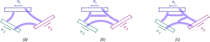
Figure 12: Typical diagrams for correlator of three Wilson frames in the leading order (a), at the one-loop level (b) and at the two-loop level (c)

There are also “mixed” poles at $\gamma_{i}=0,\gamma^{\ast}_{j},\gamma^{\ast}_{k}$ and $\gamma_{i}=0,\gamma_{j}=0,\gamma^{\ast}_{k}$. They should cancel with the contribution of diagrams of the type shown in Fig. 12 b and c (recall that our three-dipole approximations are correct starting from the $g^{6}$ diagrams of the Fig. 9a.)

Thus, the result for all diagrams (Fig. 7 + Fig. 12) is given by Eq. (111) which translates to the structure constant $C(\omega_{i},g^{2})$ given by Eq. (24)

$$F(\gamma^{\ast}_{1},\gamma^{\ast}_{2},\gamma^{\ast}_{3})~{}=~{}64g^{6}\tilde{\Lambda}(\gamma^{\ast}_{1},\gamma^{\ast}_{2},\gamma^{\ast}_{3})\prod_{k=1}^{3}{(1+\gamma_{k}^{\ast})2^{-2\gamma^{\ast}_{k}}\Gamma\big{(}2+{\gamma_{k}^{\ast}\over 2}\big{)}\Gamma\big{(}{1\over 2}-{\gamma_{k}^{\ast}\over 2}\big{)}\over\Gamma\big{(}1-{\gamma_{k}^{\ast}\over 2}\big{)}\Gamma\big{(}{3\over 2}+{\gamma_{k}^{\ast}\over 2}\big{)}{\gamma_{k}^{\ast}}^{2}\tilde{\aleph}^{\prime}(\gamma_{k}^{\ast})}$$ (114)

where $\gamma^{\ast}$ is the solution of Eq. (110) and $\tilde{\Lambda}(\gamma_{i})={\bar{\Lambda}}(-2\epsilon_{i})$ is given by Eq. (172). It is easy to see that at small $\gamma^{\ast}_{i}$ ($\Leftrightarrow~{}g^{2}\ll\omega_{i}\ll 1$)

$$F(\gamma^{\ast}_{1},\gamma^{\ast}_{2},\gamma^{\ast}_{3})~{}=~{}1+O(\gamma_{i}^{\ast})~{}=1+O\big{(}{g^{2}\over\omega_{i}}\big{)}$$ (115)

7 Conclusions

Let us summarize the results of this paper. The correlator of three “forward” light-ray operators (17) has the form

$$\langle S_{1n_{1}}^{j_{1}}(z_{1_{t}})S_{1n_{2}}^{j_{2}}(z_{2_{t}})S_{1n_{3}}^{j_{3}}(z_{3_{t}})\rangle$$ (116)

$$=~{}C(\Delta_{i},j_{i},g^{2}){(-2n_{1}\cdot n_{2})^{j_{1}+j_{2}-j_{3}-1\over 2}\over|z_{12_{t}}|^{\Delta_{1}+\Delta_{2}-\Delta_{3}-1}}{(-2n_{1}\cdot n_{3})^{j_{1}+j_{3}-j_{2}-1\over 2}\over|z_{13_{t}}|^{\Delta_{1}+\Delta_{3}-\Delta_{2}-1}}{(-2n_{2}\cdot n_{3})^{j_{2}+j_{3}-j_{1}-1\over 2}\over|z_{23_{t}}|^{\Delta_{2}+\Delta_{3}-\Delta_{1}-1}}\mu^{-\gamma_{1}-\gamma_{2}-\gamma_{3}}$$

with the structure constant

$$C(\omega_{i},g^{2})~{}=~{}{iN_{c}^{2}\omega_{1}\omega_{2}\omega_{3}F(\omega_{i},g^{2})\over\pi^{3}(\omega_{1}+\omega_{2}-\omega_{3})(\omega_{1}+\omega_{3}-\omega_{2})(\omega_{2}+\omega_{3}-\omega_{1})}$$ (117)

At small $\omega_{i}$ the operator $S_{1}^{j}$ can be identified with gluon light-ray operator ${\cal F}^{j}$ given by Eq. (15). In the tree approximation, the correlator of three gluon operators is given by Eq. (116) with $F=1+O(\omega_{i})$ as follows from Eq. (145). In the BFKL regime ($g^{2},\omega_{i}\ll 1$, ${g^{2}\over\omega_{i}}\sim 1$) the function $F$ has the form (114)

$$F(\gamma^{\ast}_{1},\gamma^{\ast}_{2},\gamma^{\ast}_{3})~{}=~{}64g^{6}\tilde{\Lambda}(\gamma^{\ast}_{1},\gamma^{\ast}_{2},\gamma^{\ast}_{3})\prod_{k=1}^{3}{(1+\gamma_{k}^{\ast})2^{-2\gamma^{\ast}_{k}}\Gamma\big{(}2+{\gamma_{k}^{\ast}\over 2}\big{)}\Gamma\big{(}{1\over 2}-{\gamma_{k}^{\ast}\over 2}\big{)}\over\Gamma\big{(}1-{\gamma_{k}^{\ast}\over 2}\big{)}\Gamma\big{(}{3\over 2}+{\gamma_{k}^{\ast}\over 2}\big{)}{\gamma_{k}^{\ast}}^{2}\tilde{\aleph}^{\prime}(\gamma_{k}^{\ast})}$$ (118)

where $\gamma^{\ast}$ is the solution of Eq. (110).

Let us now discuss main features of the result (118). First, note that since $\gamma^{\ast}$ is real, in our LLA approximation the constant $F$ is real since all the functions in the r.h.s. of Eq. (114) are real. Indeed, for $\Gamma$-functions it is trivial and for $\tilde{\Lambda}(\gamma^{\ast}_{1},\gamma^{\ast}_{2},\gamma^{\ast}_{3})$ it follows from the explicit expression (173). This is in accordance with the fact that physical s-channel imaginary part of the amplitude (68) vanishes in our approximation. Indeed, it would correspond to “cut” diagram of Fig. 13a type

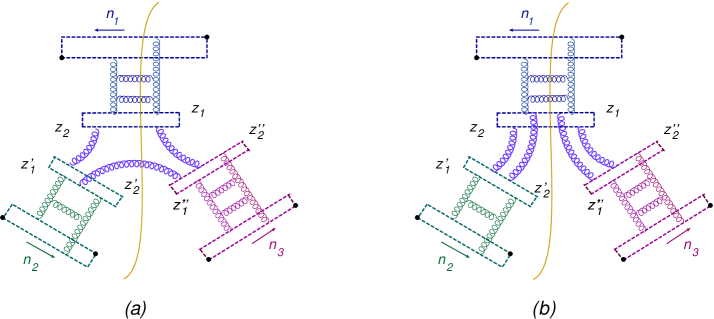
Figure 13: Typical “cut diagrams” for the correlator of three Wilson frames

and cut propagator connecting two infinite Wilson lines in $n_{2}$ and $n_{3}$ directions vanishes (see the last line in the Eq. (128) in Appendix 8.1). The imaginary part comes from the next terms of the expansion in powers of $g^{2}$ and $\omega$. The imaginary part $\sim\omega$ is given by the second term in the square brackets in the r.h.s. of tree-level expression (144). As to imaginary part $\sim g^{2}$, it comes from the diagrams of the type shown in Fig. 13b. These diagrams were calculated in the $n_{2}\rightarrow n_{3}$ limit in Refs. Balitsky:2015tca ; Balitsky:2015oux and the result is given by Eq. (157) or Eq. (159) for small $g^{2}/\omega$. Note that the result (156) has the same structure as Eq. (118).

We saw that the structure constant has poles at $\omega_{i}=\omega_{j}+\omega_{k}$ reflecting boost invariance at $n_{j}\rightarrow n_{k}$. An interesting question is what are singularities in the function $F(\omega_{i},g^{2})$ apart from obvious singular point $\omega_{i}=0$, for example like ${1\over\omega_{1}-\omega_{2}}$. It is worthwhile to note that such terms appeared in the intermediate steps in the calculation of $\Lambda$ at small ${g^{2}\over\omega_{i}}$, for example the term $J_{6}$ contains ${1\over\epsilon_{1}-\epsilon_{2}}\rightarrow{g^{2}\omega_{1}\omega_{2}\over\omega_{1}-\omega_{2}}$, see Eq. (191). There were also other singularities which all canceled in the final result (193) so it suggests that the function $F$ is finite at $\omega_{i}\neq 0$.

In conclusion, let us discuss the applicability of our results to QCD correlators of gluon light-ray operators. In the leading log approximation considered here the formulas for correlators will be the same as in ${\cal N}=4$ case since running of the coupling constant is beyond the LLA approximation, and since the contribution of scalar and gluino operators is negligible at small $\omega$. At the NLO level, in ${\cal N}=4$ case we expect only corrections to structure constant of the type of Eq. (118), but in QCD the functional form of two- and three-point correlators may change. An example of such change is the modification of the formula (41) for the $\gamma^{\ast}\gamma^{\ast}$ amplitude in QCD calculated at the NLO BFKL level in Ref. Chirilli:2013kca ; Chirilli:2014dcb . It would be interesting to write down such modifications for the correlators of gluon-light-ray operators at the NLO BFKL level in QCD.

The author is grateful to V. Kazakov, G. Korchemsky, and E. Sobko for valuable discussions. This work is supported by contract DE-AC05-06OR23177 under which the Jefferson Science Associates, LLC operate the Thomas Jefferson National Accelerator Facility, and by the grant DE-FG02-97ER41028.

8 Appendix

8.1 BFKL kernel in the triple Regge limit

In this Section I will demonstrate how the BFKL kernel comes out of the conventional momentum-space calculation in the triple Regge limit. Let us again consider the first diagram in Fig. 9. Our LLA approximation (86) in the momentum space reads

$$\alpha\beta s_{12}\gg m_{\perp}^{2},~{}~{}~{}~{}\alpha\gamma s_{13}\gg m_{\perp}^{2},~{}~{}~{}~{}\beta\gamma s_{23}\gg m_{\perp}^{2}$$ (119)

If all $s_{ij}$ are of the same order, this translates to $\alpha\gg m_{\perp}\sqrt{s_{23}\over s_{12}s_{13}}$ etc. Suppose now that we already performed integrals over $\beta$ and $\gamma$ which results in logs multiplied by (conformal) dipoles and we would like to consider the last integral over $\alpha$ coming from the diagrams of Fig. 14 type.

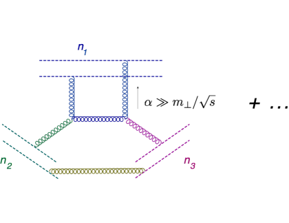
Figure 14: Leading diagrams with logarithmic integrals over $\alpha$

To avoid cluttering of formulas, we will disregard the bottom gluon connecting Wilson lines parallel to $n_{2}$ and $n_{3}$. Indeed, the corresponding factor

$$\langle{V}(z_{3t}e_{t}+\breve{z}_{3}\breve{e}){W}(z_{5t}e_{t}+{\check{z}}_{5}{\check{e}})\rangle~{}=~{}i\alpha_{s}t^{a}\otimes t^{a}\ln[z_{35t}^{2}+(\breve{z}_{3}+{\check{z}}_{5})^{2}]$$

(plus permutations) simply multiplies contributions of diagrams in Fig. 15 and has nothing to do with logarithm coming out of $\alpha$ integration.

To simplify our formulas, let us calculate the “cut diagram” shown in Fig. 15. It can be represented by a functional integral over double set of variables: fields to the left and to the right of the cut which coincide at $t=\infty$.

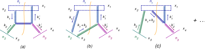
Figure 15: First rung of the BFKL evolution in the triple Regge limit

We get

$$\langle{\rm Tr}\{{\tilde{U}}^{\dagger}(x_{1})U(x_{1})U^{\dagger}(x_{2}){\tilde{U}}(x_{2})\}{\tilde{V}}^{\dagger}(x_{3})W(x_{4})\rangle$$ (120)

$$=~{}g_{{}_{\rm YM}}^{6}N_{c}t^{a}\otimes t^{a}\!\int\!{\textstyle d}\lower 0.12915pt\hbox{\kern-3.80005pt${}^{\scriptstyle-}$}\kern-0.50003pt{}^{4}k_{1}{\textstyle d}\lower 0.12915pt\hbox{\kern-3.80005pt${}^{\scriptstyle-}$}\kern-0.50003pt{}^{4}k^{\prime}_{1}{\textstyle d}\lower 0.12915pt\hbox{\kern-3.80005pt${}^{\scriptstyle-}$}\kern-0.50003pt{}^{4}k_{2}{\textstyle d}\lower 0.12915pt\hbox{\kern-3.80005pt${}^{\scriptstyle-}$}\kern-0.50003pt{}^{4}k^{\prime}_{2}~{}{\textstyle\delta}\lower 0.12915pt\hbox{\kern-3.80005pt${}^{\scriptstyle-}$}\kern-0.50003pt{}^{4}(k_{2}+k_{1}-k^{\prime}_{2}-k^{\prime}_{1})~{}{\textstyle\delta}\lower 0.12915pt\hbox{\kern-3.80005pt${}^{\scriptstyle-}$}\kern-0.50003pt{}((k_{2}+k_{1})^{2})\theta(k_{2}+k_{1})_{0}$$

$$\times~{}{\textstyle\delta}\lower 0.12915pt\hbox{\kern-3.80005pt${}^{\scriptstyle-}$}\kern-0.50003pt{}(k_{2}\cdot n_{2}){\textstyle\delta}\lower 0.12915pt\hbox{\kern-3.80005pt${}^{\scriptstyle-}$}\kern-0.50003pt{}(k_{1}\cdot n_{1}){\textstyle\delta}\lower 0.12915pt\hbox{\kern-3.80005pt${}^{\scriptstyle-}$}\kern-0.50003pt{}(k^{\prime}_{2}\cdot n_{3}){\textstyle\delta}\lower 0.12915pt\hbox{\kern-3.80005pt${}^{\scriptstyle-}$}\kern-0.50003pt{}(k^{\prime}_{1}\cdot n_{1})~{}{L^{\lambda}(k_{2},k_{1})L_{\lambda}(k^{\prime}_{2},k^{\prime}_{1})\over k_{1}^{2}k_{2}^{2}{k^{\prime}}_{1}^{2}{k^{\prime}}_{2}^{2}}~{}e^{ik_{2t}x_{3t}+i\breve{k}_{2}\breve{x}_{3}}$$

$$\times~{}\big{(}e^{ik_{1t}x_{1t}+i{\tilde{k}}_{1}{\tilde{x}}_{1}}-e^{ik_{1t}x_{2t}+i{\tilde{k}}_{1}{\tilde{x}}_{2}}\big{)}e^{-ik^{\prime}_{2t}x_{4t}-i{\check{k}}^{\prime}_{2}\check{x}_{4}}\big{(}e^{-ik^{\prime}_{1t}x_{1t}-i{\tilde{k}}^{\prime}_{1}{\tilde{x}}_{1}}-e^{-ik^{\prime}_{1t}x_{2t}-i{\tilde{k}}^{\prime}_{1}{\tilde{x}}_{2}}\big{)}$$

where we denoted Wilson lines to the left of the cut by tilde. Here we use space-saving notations ${\textstyle d}\lower 0.12915pt\hbox{\kern-3.80005pt${}^{\scriptstyle-}$}\kern-0.50003pt{}^{n}k\equiv{d^{n}k\over(2\pi)^{n}}$ and ${\textstyle\delta}\lower 0.12915pt\hbox{\kern-3.80005pt${}^{\scriptstyle-}$}\kern-0.50003pt{}^{(n)}(k)\equiv(2\pi)^{n}\delta^{(n)}(k)$. The Lipatov vertex of gluon emission can be taken e.g. from Ref. Babansky:2002my

$${2\over s_{12}}L(k_{2},k_{1}) = (k_{1}-k_{2})-\Big{[}2{k_{1n_{2}}\over n_{12}}+{k_{1}^{2}\over k_{2n_{1}}}\Big{]}n_{1}+\Big{[}2{k_{2n_{1}}\over n_{12}}+{k_{2}^{2}\over k_{1n_{2}}}\Big{]}n_{2}$$

$${2\over s_{13}}L(k^{\prime}_{2},k^{\prime}_{1}) = (k^{\prime}_{1}-k^{\prime}_{2})-\Big{[}2{k^{\prime}_{1n_{3}}\over n_{13}}+{{k^{\prime}}_{1}^{2}\over k^{\prime}_{2n_{1}}}\Big{]}n_{1}+\Big{[}2{k^{\prime}_{2n_{1}}\over n_{13}}+{{k^{\prime}}_{2}^{2}\over k^{\prime}_{1n_{3}}}\Big{]}n_{3}$$ (121)

Rewriting these formulas in terms of triple Sudakov variables (69) and taking into account $\delta$-functions in the r.h.s. of Eq. (120) we obtain

$${2\over s_{12}}L(k_{1},k_{2})~{}=~{}(k_{1}-k_{2})_{t}+$$ (122)

$$+~{}n_{1}\Big{[}-\alpha_{1}-\alpha_{2}-{k_{1}^{2}\over k_{2n_{1}}}-2\gamma_{1}{n_{23}\over n_{12}}\Big{]}+n_{2}\Big{[}\beta_{1}+\beta_{2}+{k_{2}^{2}\over k_{1n_{2}}}+2\gamma_{2}{n_{13}\over n_{12}}\Big{]}+(\gamma_{1}-\gamma_{2})n_{3}$$

$${2\over s_{13}}L(k^{\prime}_{1},k^{\prime}_{2})~{}=~{}(k^{\prime}_{1}-k^{\prime}_{2})_{t}$$

$$+~{}n_{1}\Big{[}-\alpha^{\prime}_{1}-\alpha^{\prime}_{2}-{{k^{\prime}}_{1}^{2}\over k_{2n_{1}}}-2\beta^{\prime}_{1}{n_{23}\over n_{13}}\Big{]}+(\beta^{\prime}_{1}-\beta^{\prime}_{2})n_{2}+n_{3}\Big{[}\gamma^{\prime}_{1}+\gamma^{\prime}_{2}+{{k^{\prime}}_{2}^{2}\over k^{\prime}_{1n_{3}}}+2\beta^{\prime}_{2}{n_{12}\over n_{13}}\Big{]}$$

In our LLA approximation $\alpha_{1}\gg m\sqrt{s_{23}\over s_{12}s_{13}}$ and $\beta_{1}\sim\beta^{\prime}_{1}\sim\beta^{\prime}_{2}\sim m\sqrt{s_{13}\over s_{12}s_{23}}$, $\alpha_{2}\sim\alpha^{\prime}_{2}\sim m\sqrt{s_{23}\over s_{12}s_{13}}$, $\gamma_{1}\sim\gamma_{2}\sim m\sqrt{s_{12}\over s_{13}s_{23}}$. Moreover, from $\delta$-function $\delta((k_{2}+k_{1})^{2})\theta(k_{2}+k_{1})_{0}$ we see that $\xi_{2}=\beta_{2}-\alpha_{2}{s_{13}\over s_{23}}={s_{13}\over s_{12}}\big{(}\gamma^{\prime}_{2}-\alpha^{\prime}_{2}{s_{12}\over s_{23}}\big{)}\ll{m\over\sqrt{s}}$. Using these approximations, one obtains after some algebra

$${2\over s_{12}s_{13}}L(k_{2},k_{1})L(k^{\prime}_{2},k^{\prime}_{1})~{}=~{}-(k_{1}-k^{\prime}_{1})_{t}^{2}-{s_{12}s_{23}\over s_{13}}(\beta_{1}-\beta^{\prime}_{1})^{2}$$ (123)

$$+~{}{\big{(}k_{1t}^{2}+{s_{12}s_{23}\over s_{13}}\beta_{1}^{2}\big{)}\big{(}{k^{\prime}_{2t}}^{2}+{s_{12}s_{23}\over s_{13}}{\beta^{\prime}}_{2}^{2}\big{)}\over(k_{1}+k_{2})_{t}^{2}+{s_{12}s_{23}\over s_{13}}(\beta_{1}+\beta_{2})^{2}}+{\big{(}k_{2t}^{2}+{s_{12}s_{23}\over s_{13}}\beta_{2}^{2}\big{)}\big{(}{k^{\prime}_{1t}}^{2}+{s_{12}s_{23}\over s_{13}}{\beta^{\prime}}_{1}^{2}\big{)}\over(k_{1}+k_{2})_{t}^{2}+{s_{12}s_{23}\over s_{13}}(\beta_{1}+\beta_{2})^{2}}~{}+~{}O\big{(}{k_{t}^{2}\over\alpha_{1}s}\big{)}$$

which is a “real part” of the BFKL kernel.

The amplitude can be rewtitten as

$$\langle{\rm Tr}\{{\tilde{U}}^{\dagger}(x_{1})U(x_{1})U^{\dagger}(x_{2}){\tilde{U}}(x_{2})\}{\tilde{V}}^{\dagger}(x_{3})W(x_{4})\rangle$$ (124)

$$=~{}{g_{{}_{\rm YM}}^{6}N_{c}\over 4\pi}t^{a}\otimes t^{a}\!\int_{0}^{\infty}\!{d\alpha_{1}\over\alpha_{1}}\!\int\!{\textstyle d}\lower 0.12915pt\hbox{\kern-3.80005pt${}^{\scriptstyle-}$}\kern-0.50003pt{}k_{1t}{\textstyle d}\lower 0.12915pt\hbox{\kern-3.80005pt${}^{\scriptstyle-}$}\kern-0.50003pt{}k^{\prime}_{1t}{\textstyle d}\lower 0.12915pt\hbox{\kern-3.80005pt${}^{\scriptstyle-}$}\kern-0.50003pt{}k_{2t}{\textstyle d}\lower 0.12915pt\hbox{\kern-3.80005pt${}^{\scriptstyle-}$}\kern-0.50003pt{}k^{\prime}_{2t}~{}{\textstyle\delta}\lower 0.12915pt\hbox{\kern-3.80005pt${}^{\scriptstyle-}$}\kern-0.50003pt{}(k_{1}+k_{2}-k^{\prime}_{1}-k^{\prime}_{2})_{t}$$

$$\times~{}\int\!{\textstyle d}\lower 0.12915pt\hbox{\kern-3.80005pt${}^{\scriptstyle-}$}\kern-0.50003pt{}{\tilde{k}}_{1}{\textstyle d}\lower 0.12915pt\hbox{\kern-3.80005pt${}^{\scriptstyle-}$}\kern-0.50003pt{}{\tilde{k}}^{\prime}_{1}{\textstyle d}\lower 0.12915pt\hbox{\kern-3.80005pt${}^{\scriptstyle-}$}\kern-0.50003pt{}\breve{k}_{2}{\textstyle d}\lower 0.12915pt\hbox{\kern-3.80005pt${}^{\scriptstyle-}$}\kern-0.50003pt{}{\check{k}}^{\prime}_{2}~{}{\textstyle\delta}\lower 0.12915pt\hbox{\kern-3.80005pt${}^{\scriptstyle-}$}\kern-0.50003pt{}\big{(}{\tilde{k}}_{1}-\breve{k}_{2}-{\tilde{k}}^{\prime}_{1}+{\check{k}}^{\prime}_{2}\big{)}$$

$$\times~{}\big{(}e^{ik_{1t}x_{1t}+i{\tilde{k}}_{1}{\tilde{x}}_{1}}-e^{ik_{1t}x_{2t}+i{\tilde{k}}_{1}{\tilde{x}}_{2}}\big{)}\big{(}e^{-i(k^{\prime}_{1},x_{1})_{t}}-e^{-i(k^{\prime}_{1},x_{2})_{t}}\big{)}e^{ik_{2t}x_{3t}+i\breve{k}_{2}\breve{x}_{3}}e^{-ik^{\prime}_{2t}x_{4t}-i{\check{k}}^{\prime}_{2}\check{x}_{4}}$$

$$\times~{}{-(k_{1}-k^{\prime}_{1})_{t}^{2}-({\tilde{k}}_{1}-{\tilde{k}}^{\prime}_{1})^{2}+{(k_{1t}^{2}+{\tilde{k}}_{1}^{2})({k^{\prime}}_{2t}^{2}+\tilde{k^{\prime}}_{2}^{2})+(k_{2t}^{2}+{\tilde{k}}_{2}^{2})({k^{\prime}}_{1t}^{2}+\tilde{k^{\prime}}_{1}^{2})\over(k_{1}+k^{\prime}_{1})_{t}^{2}+({\tilde{k}}_{1}+{\tilde{k}}^{\prime}_{1})^{2}}\over(k_{1t}^{2}+{\tilde{k}}_{1}^{2})({k^{\prime}}_{1t}^{2}+{\tilde{k^{\prime}}}_{1}^{2})(k_{2t}^{2}+\breve{k}_{2}^{2})({k^{\prime}}_{2t}^{2}+{\check{k^{\prime}}_{2}}^{2})}$$

Note that at $n_{2}=n_{3}$ this formula reduces to the first rung of the BFKL ladder for dipole-dipole cross section Babansky:2002my

In this form it coincides with the first iteration of the evolution equation for color dipoles. Let us demonstrate this for the simple term in the BFKL kernel $2k_{1t}k^{\prime}_{1t}+2{\tilde{k}}_{1}{\tilde{k}}^{\prime}_{1}$. Performing momentum integrals one obtains

$${g_{{}_{\rm YM}}^{6}N_{c}\over 4\pi}t^{a}\otimes t^{a}\!\int_{0}^{\infty}\!{d\alpha_{1}\over\alpha_{1}}\!\int\!{\textstyle d}\lower 0.12915pt\hbox{\kern-3.80005pt${}^{\scriptstyle-}$}\kern-0.50003pt{}k_{1t}{\textstyle d}\lower 0.12915pt\hbox{\kern-3.80005pt${}^{\scriptstyle-}$}\kern-0.50003pt{}k^{\prime}_{1t}{\textstyle d}\lower 0.12915pt\hbox{\kern-3.80005pt${}^{\scriptstyle-}$}\kern-0.50003pt{}k_{2t}{\textstyle d}\lower 0.12915pt\hbox{\kern-3.80005pt${}^{\scriptstyle-}$}\kern-0.50003pt{}k^{\prime}_{2t}~{}{\textstyle\delta}\lower 0.12915pt\hbox{\kern-3.80005pt${}^{\scriptstyle-}$}\kern-0.50003pt{}(k_{1}+k_{2}-k^{\prime}_{1}-k^{\prime}_{2})_{t}$$ (125)

$$\times~{}\int\!{\textstyle d}\lower 0.12915pt\hbox{\kern-3.80005pt${}^{\scriptstyle-}$}\kern-0.50003pt{}{\tilde{k}}_{1}{\textstyle d}\lower 0.12915pt\hbox{\kern-3.80005pt${}^{\scriptstyle-}$}\kern-0.50003pt{}{\tilde{k}}^{\prime}_{1}{\textstyle d}\lower 0.12915pt\hbox{\kern-3.80005pt${}^{\scriptstyle-}$}\kern-0.50003pt{}\breve{k}_{2}{\textstyle d}\lower 0.12915pt\hbox{\kern-3.80005pt${}^{\scriptstyle-}$}\kern-0.50003pt{}{\check{k}}^{\prime}_{2}~{}{\textstyle\delta}\lower 0.12915pt\hbox{\kern-3.80005pt${}^{\scriptstyle-}$}\kern-0.50003pt{}\big{(}{\tilde{k}}_{1}-\breve{k}_{2}-{\tilde{k}}^{\prime}_{1}+{\check{k}}^{\prime}_{2}\big{)}{2k_{1t}k^{\prime}_{1t}+2{\tilde{k}}_{1}{\tilde{k}}^{\prime}_{1}\over(k_{1t}^{2}+{\tilde{k}}_{1}^{2})({k^{\prime}}_{1t}^{2}+{\tilde{k^{\prime}}}_{1}^{2})(k_{2t}^{2}+\breve{k}_{2}^{2})({k^{\prime}}_{2t}^{2}+{\check{k^{\prime}}_{2}}^{2})}$$

$$\times~{}\big{(}e^{ik_{1t}x_{1t}+i{\tilde{k}}_{1}{\tilde{x}}_{1}}-e^{ik_{1t}x_{2t}+i{\tilde{k}}_{1}{\tilde{x}}_{2}}\big{)}\big{(}e^{-i(k^{\prime}_{1},x_{1})_{t}}-e^{-i(k^{\prime}_{1},x_{2})_{t}}\big{)}e^{ik_{2t}x_{3t}+i\breve{k}_{2}\breve{x}_{3}}e^{-ik^{\prime}_{2t}x_{4t}-i{\check{k}}^{\prime}_{2}\check{x}_{4}}$$

$$=~{}{\alpha_{s}^{3}N_{c}\over 2\pi^{2}}t^{a}\otimes t^{a}\!\int_{0}^{\infty}\!{d\alpha_{1}\over\alpha_{1}}$$

$$\hskip 31.29802pt\times~{}\!\int\!d^{2}z_{\perp}{(x_{1}-x_{2})_{\perp}^{2}\over(x_{1}-z)^{2}(x_{2}-z)^{2}}\ln[(x_{3t}-z_{t})^{2}+(\breve{x}_{3}+{\tilde{z}})^{2}]\ln[(x_{4t}-z_{t})^{2}+(\check{x}_{4}+{\tilde{z}})^{2}]$$

where $z_{\perp}\equiv z_{t},{\tilde{z}}$.

On the other hand, the (linearized) evolution equation for color dipoles (in the double functional integral formalism) reads Balitsky:1997mk ; Balitsky:2001gj

$${d\over dY}{\rm Tr}\{{\tilde{U}}^{\dagger}(x_{1})U(x_{1})U^{\dagger}(x_{2}){\tilde{U}}(x_{2})\}~{}$$

$$=~{}{\alpha_{s}N_{c}\over 2\pi}\!\int\!d^{2}z_{\perp}~{}{(x_{1}-x_{2})_{\perp}^{2}\over(x_{1}-z)_{\perp}^{2}(x_{2}-z)_{\perp}^{2}}\big{[}{\rm Tr}\{{\tilde{U}}^{\dagger}(x_{1})U(x_{1})U^{\dagger}(z){\tilde{U}}(z)\}$$

$$+~{}{\rm Tr}\{{\tilde{U}}^{\dagger}(z)U(z)U^{\dagger}(x_{2}){\tilde{U}}(x_{2})\}-{\rm Tr}\{{\tilde{U}}^{\dagger}(x_{1})U(x_{1})U^{\dagger}(x_{2}){\tilde{U}}(x_{2})\}\big{]}$$ (126)

where $Y\equiv\ln\alpha$. The term (125) comes from the correlator

$${\alpha_{s}N_{c}\over 2\pi}\!\int_{0}^{\infty}\!{d\alpha\over\alpha}\!\int\!d^{2}z_{\perp}~{}{-2(x_{1}-z,x_{2}-z)_{\perp}\over(x_{1}-z)_{\perp}^{2}(x_{2}-z)_{\perp}^{2}}$$

$$\hskip 93.89409pt\times~{}\langle{\rm Tr}\{U^{\dagger}(z){\tilde{U}}(z)+{\tilde{U}}^{\dagger}(z)U(z)\}{\tilde{V}}^{\dagger}(x_{3})W(x_{4})\rangle$$ (127)

Using the tree-level correlators of Wilson lines

$$\langle\tilde{U}(z_{t}e_{t}+{\tilde{z}}{\tilde{e}})\tilde{V}(x_{3t}e_{t}+\breve{x}_{3}\breve{e})\rangle~{}=~{}i\alpha_{s}t^{a}\otimes t^{a}\ln[(z-x_{3})_{t}^{2}+({\tilde{z}}+\breve{x}_{3})^{2}],$$

$$\langle{U}(z_{t}e_{t}+{\tilde{z}}{\tilde{e}}){W}(x_{4t}e_{t}+{\check{z}}_{4}{\check{e}})\rangle~{}=~{}-i\alpha_{s}t^{a}\otimes t^{a}\ln[(z-x_{4})_{t}^{2}+({\tilde{z}}+\check{x}_{4})^{2}],$$

$$\langle\tilde{U}(z_{t}e_{t}+{\tilde{z}}{\tilde{e}}){W}(x_{4t}e_{t}+\check{x}_{4}{\check{e}})\rangle~{}=~{}\langle U(z_{t}e_{t}+{\tilde{z}}{\tilde{e}})\tilde{V}(x_{3t}e_{t}+\check{x}_{3}{\check{e}})\rangle~{}=~{}0$$ (128)

it is easy to see that Eq.(127) coincides with the r.h.s. of Eq. (125). Similarly, one can check that other terms in the BFKL kernel correspond to linear part of the evolution equation for color dipoles (126), see e.g. the book Kovchegov:2012mbw .

8.2 Correlator of three twist-2 LR operators in the tree approximation

First, we calculate the correlator of two light-ray gluon operators. Using bare propagator

$$\pi^{2}\langle F_{n_{1}}^{~{}\mu}(u_{1}n_{1}+x_{1_{\perp}})F_{n_{2}}^{~{}\nu}(u_{2}n_{2}+x_{2_{\perp}})\rangle$$ (129)

$$=~{}-{g^{\mu\nu}\delta^{ab}s_{12}x_{12_{\perp}}^{2}\over 2(u_{1}u_{2}s_{12}+x_{12_{\perp}}^{2}+i\epsilon)^{3}}-{\delta^{ab}n_{2}^{\mu}n_{1}^{\nu}\over(u_{1}u_{2}s_{12}+x_{12_{\perp}}^{2}+i\epsilon)^{2}}$$

$$\hskip 14.22636pt-~{}{s_{12}\delta^{ab}\over(u_{1}u_{2}s_{12}+x_{12_{\perp}}^{2}+i\epsilon)^{3}}\big{[}u_{2}x_{12}^{\mu}n_{2}^{\nu}-u_{1}n_{1}^{\mu}x_{12}^{\nu}-x_{12}^{\mu}x_{12}^{\nu}+u_{1}u_{2}(n_{1}^{\mu}n_{2}^{\nu}-n_{2}^{\mu}n_{1}^{\nu})\big{]}$$

after simple integration we get the tree-level correlator in the form

$${1\over N_{c}^{2}-1}\langle{\cal F}^{j}_{n_{1}}(x_{1_{\perp}}){\cal F}^{j^{\prime}}_{n_{2}}(x_{2_{\perp}})\big{\rangle}~{}=~{}-{is^{4}\over 2\pi}\delta(\omega-\omega^{\prime}){1-e^{i\pi\omega}\over\sin\pi\omega}{\omega(1+\omega)\over(x_{12_{\perp}}^{2})^{2+\omega}s^{-\omega}}{\Gamma(2+\omega)\Gamma(4+\omega)\over\Gamma(4+2\omega)}$$ (130)

which agrees with Eq. (67) in the limit $\omega\rightarrow 0$

$${1\over N_{c}^{2}-1}\langle{\cal F}^{j}_{n_{1}}(x_{1_{\perp}}){\cal F}^{j^{\prime}}_{n_{2}}(x_{2_{\perp}})\big{\rangle}~{}\simeq~{}-\delta(j-j^{\prime}){\omega\over 2\pi x_{12_{\perp}}^{4}}{s^{\omega}\over x_{12_{\perp}}^{2\omega}}$$ (131)

as discussed in the end of Sect. 5.2.

Next, consider diagrams in Fig. 16 representing the 3-point correlator of gluon light-ray operators in the leading perturbative order.

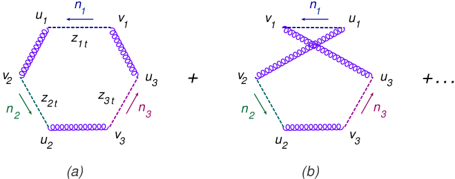
Figure 16: Tree-level correlator of three twist-two gluon LR operators

After some algebra one obtains the result for the first diagram in Fig. 16a in the form

$$\langle F_{n_{1}}^{a\mu}(u_{1}n_{1}+z_{1t})F_{n_{2}}^{b~{}\nu}(v_{2}n_{2}+z_{2t})\rangle\langle F^{a}_{n_{1}\mu}(v_{1}n_{1}+z_{1t})F_{n_{3}}^{c\lambda}(u_{3}n_{3}+z_{3t})\rangle$$

$$\hskip 93.89409pt\times~{}\langle F^{b}_{n_{2}\nu}(u_{2}n_{2}+z_{2t})F^{c}_{n_{3}\lambda}(v_{3}n_{3}+z_{3t})\rangle~{}$$

$$=~{}{N_{c}^{2}-1\over 4\pi^{6}s_{12}s_{23}s_{13}}{z_{12_{t}}^{2}z_{13_{t}}^{2}z_{23_{t}}^{2}\over(u_{1}v_{2}s_{12}+z_{12_{t}}^{2}+i\epsilon)^{3}(v_{1}u_{3}s_{13}+z_{13_{t}}^{2}+i\epsilon)^{3}(u_{2}v_{3}s_{23}+z_{23_{t}}^{2}+i\epsilon)^{3}}$$

(132)

where $s_{12}\equiv-2n_{1}\cdot n_{2}$ etc. Adding the diagrams with permutations we obtain

$$\int_{-\infty}^{\infty}\!du_{1}dv_{1}du_{2}dv_{2}du_{3}dv_{3}~{}\theta(u_{1}-v_{1})\theta(u_{2}-v_{2})\theta(u_{3}-v_{3})~{}$$

$$\hskip 31.29802pt\times~{}(u_{1}-v_{1})^{-\omega_{1}}(u_{2}-v_{2})^{-\omega_{2}}(u_{3}-v_{3})^{-\omega_{3}}\langle F_{n_{1}}^{a\mu}(u_{1}n_{1}+z_{1t})F^{a}_{n_{1}\mu}(v_{1}n_{1}+z_{1t})$$

$$\hskip 31.29802pt\times~{}F_{n_{2}}^{b~{}\nu}(v_{2}n_{2}+z_{2t})F^{b}_{n_{2}\nu}(u_{2}n_{2}+z_{2t})F_{n_{3}}^{c\lambda}(u_{3}n_{3}+z_{3t})F^{c}_{n_{3}\lambda}(v_{3}n_{3}+z_{3t})\rangle~{}$$

$$=~{}{N_{c}^{2}-1\over 4\pi^{6}s_{12}s_{23}s_{13}}\int_{-\infty}^{\infty}\!du_{1}dv_{1}du_{2}dv_{2}du_{3}dv_{3}~{}\big{[}\theta(u_{1}-v_{1})(u_{1}-v_{1})^{-\omega_{1}}+u_{1}\leftrightarrow v_{1}\big{]}$$

$$\hskip 31.29802pt\times~{}\big{[}\theta(u_{2}-v_{2})(u_{2}-v_{2})^{-\omega_{2}}+u_{2}\leftrightarrow v_{2}\big{]}\big{[}\theta(u_{3}-v_{3})(u_{3}-v_{3})^{-\omega_{3}}+u_{3}\leftrightarrow v_{3}\big{]}$$

$$\hskip 31.29802pt{z_{12_{t}}^{2}z_{13_{t}}^{2}z_{23_{t}}^{2}\over\times~{}(u_{1}v_{2}s_{12}+z_{12_{t}}^{2}+i\epsilon)^{3}(v_{1}u_{3}s_{13}+z_{13_{t}}^{2}+i\epsilon)^{3}(u_{2}v_{3}s_{23}+z_{23_{t}}^{2}+i\epsilon)^{3}}$$

(133)

The integration over light-ray variables $u_{i},v_{i}$ is done with the help of two formulas:

$$\int_{-\infty}^{\infty}\!dt_{1}dt_{2}dt_{3}\!\int_{0}^{\infty}\!dr_{1}dr_{2}dr_{3}{1\over[(r_{1}+t_{1})(r_{2}+t_{2})+a_{12}^{2}+i\epsilon]}$$ (134)

$$\times~{}\Big{\{}{r_{1}^{-\omega_{1}}r_{2}^{-\omega_{2}}r_{3}^{-\omega_{3}}\over[t_{1}(r_{3}+t_{3})+a_{13}^{2}+i\epsilon](t_{2}t_{3}+a_{23}^{2}+i\epsilon)}+{r_{1}^{-\omega_{1}}r_{2}^{-\omega_{2}}r_{3}^{-\omega_{3}}\over(t_{1}t_{3}+a_{13}^{2}+i\epsilon)[t_{2}(r_{3}+t_{3})+a_{23}^{2}+i\epsilon]}\Big{\}}$$

$$=-4\sin{\pi\omega_{3}\over 2}\sin{\pi\over 2}(\omega_{1}+\omega_{2}-\omega_{3})\cos{\pi\over 2}(\omega_{1}-\omega_{2})\Gamma(1-\omega_{1})\Gamma(1-\omega_{2})\Gamma(1-\omega_{3})$$

$$\times~{}\Gamma^{2}\big{(}{\omega_{1}+\omega_{2}-\omega_{3}\over 2}\big{)}\Gamma^{2}\big{(}{\omega_{2}+\omega_{3}-\omega_{1}\over 2}\big{)}\Gamma^{2}\big{(}{\omega_{1}+\omega_{3}-\omega_{2}\over 2}\big{)}a_{12}^{\omega_{3}-\omega_{1}-\omega_{2}}a_{13}^{\omega_{2}-\omega_{1}-\omega_{3}}a_{23}^{\omega_{1}-\omega_{2}-\omega_{3}}$$

and

$$\int_{-\infty}^{\infty}\!dt_{1}dt_{2}dt_{3}\!\int_{0}^{\infty}\!dr_{1}dr_{2}dr_{3}$$

$$\times~{}\Big{[}{r_{1}^{-\omega_{1}}r_{2}^{-\omega_{2}}r_{3}^{-\omega_{3}}\over[(r_{1}+t_{1})t_{2}+a_{12}+i\epsilon][t_{1}(r_{3}+t_{3})+a_{13}+i\epsilon][(r_{2}+t_{2})t_{3}+a_{23}+i\epsilon]}$$

$$\hskip 31.29802pt+~{}{r_{1}^{-\omega_{1}}r_{2}^{-\omega_{2}}r_{3}^{-\omega_{3}}\over[t_{1}(r_{2}+t_{2})+a_{12}+i\epsilon][(r_{1}+t_{1})t_{3}+a_{13}+i\epsilon][t_{2}(r_{3}+t_{3})+a_{23}+i\epsilon]}\Big{]}$$

$$=~{}\Gamma(1-\omega_{1})\Gamma(1-\omega_{2})\Gamma(1-\omega_{3})\Gamma^{2}\big{(}{\omega_{1}+\omega_{3}-\omega_{2}\over 2}\big{)}\Gamma^{2}\big{(}{\omega_{2}+\omega_{3}-\omega_{1}\over 2}\big{)}\Gamma^{2}\big{(}{\omega_{1}+\omega_{2}-\omega_{3}\over 2}\big{)}$$

$$\hskip 31.29802pt\times~{}a_{12}^{\omega_{3}-\omega_{1}-\omega_{2}}a_{13}^{\omega_{2}-\omega_{1}-\omega_{3}}a_{23}^{\omega_{1}-\omega_{2}-\omega_{3}}$$

$$\hskip 31.29802pt\times~{}\big{[}e^{i\pi(\omega_{1}+\omega_{2}-\omega_{3})}+e^{i\pi(\omega_{2}+\omega_{3}-\omega_{1})}+e^{i\pi(\omega_{1}+\omega_{3}-\omega_{2})}-e^{i\pi(\omega_{1}+\omega_{2}+\omega_{3})}-2\big{]}$$ (135)

Using these formulas with $a^{2}_{ij}={z_{ij_{t}}^{2}\over s_{i}j}$ it is easy to get

$$\int_{-\infty}^{\infty}\!du_{1}dv_{1}\big{[}(u_{1}-v_{1})^{-\omega_{1}}\theta(u_{1}-v_{1})+u_{1}\leftrightarrow v_{1}\big{]}\!\int_{-\infty}^{\infty}\!du_{2}dv_{2}\big{[}(u_{2}-v_{2})^{-\omega_{2}}\theta(u_{2}-v_{2})$$ (136)

$$+~{}u_{2}\leftrightarrow v_{2}\big{]}\!\int_{-\infty}^{\infty}\!du_{3}dv_{3}\big{[}(u_{3}-v_{3})^{-\omega_{3}}\theta(u_{3}-v_{3})+u_{3}\leftrightarrow v_{3}\big{]}$$

$$\hskip 31.29802pt\times~{}{1\over(u_{1}v_{2}s_{12}+z_{12}^{2}+i\epsilon)(v_{1}u_{3}s_{13}+z_{13}^{2}+i\epsilon)(u_{2}v_{3}s_{23}+z_{23}^{2}+i\epsilon)}$$

$$=~{}{1\over s_{12}s_{13}s_{23}}\Phi(\omega_{1},\omega_{2},\omega_{3})\Gamma(1-\omega_{1})\Gamma(1-\omega_{2})\Gamma(1-\omega_{3})\Gamma^{2}\big{(}{\omega_{1}+\omega_{2}-\omega_{3}\over 2}\big{)}$$

$$\hskip 31.29802pt\times~{}\Gamma^{2}\big{(}{\omega_{2}+\omega_{3}-\omega_{1}\over 2}\big{)}\Gamma^{2}\big{(}{\omega_{1}+\omega_{3}-\omega_{2}\over 2}\big{)}\big{(}{s_{12}\over z_{12}^{2}}\big{)}^{\omega_{1}+\omega_{2}-\omega_{3}\over 2}\big{(}{s_{13}\over z_{13}^{2}}\big{)}^{\omega_{1}+\omega_{3}-\omega_{2}\over 2}\big{(}{s_{23}\over z_{23}^{2}}\big{)}^{\omega_{2}+\omega_{3}-\omega_{1}\over 2}$$

where

$$\Phi(\omega_{1},\omega_{2},\omega_{3})~{}$$

$$=~{}-4\sin{\pi\omega_{1}\over 2}\sin{\pi\over 2}(\omega_{2}+\omega_{3}-\omega_{1})\cos{\pi\over 2}(\omega_{2}-\omega_{3})-4\sin{\pi\omega_{2}\over 2}\sin{\pi\over 2}(\omega_{1}+\omega_{3}-\omega_{2})$$

$$\times~{}\cos{\pi\over 2}(\omega_{1}-\omega_{3})-4\sin{\pi\omega_{3}\over 2}\sin{\pi\over 2}(\omega_{1}+\omega_{2}-\omega_{3})\cos{\pi\over 2}(\omega_{1}-\omega_{2})$$

$$+~{}e^{i\pi(\omega_{1}+\omega_{2}-\omega_{3})}+e^{i\pi(\omega_{2}+\omega_{3}-\omega_{1})}+e^{i\pi(\omega_{1}+\omega_{3}-\omega_{2})}-e^{i\pi(\omega_{1}+\omega_{2}+\omega_{3})}-2$$ (137)

Now, differentiating Eq. (136) two times with respect to each $x_{ij_{t}}^{2}$ one obtains

$$\langle{\cal F}_{n_{1}}(\omega_{1},z_{1_{t}}){\cal F}_{\omega_{2},n_{2}}(z_{2_{t}}){\cal F}_{\omega_{3},n_{3}}(z_{3_{t}})\rangle~{}$$

$$=~{}{N_{c}^{2}-1\over 32\pi^{6}z_{12}^{2}z_{13}^{2}z_{23}^{2}}\Gamma\big{(}{\omega_{1}+\omega_{2}-\omega_{3}\over 2}\big{)}\Gamma\big{(}{\omega_{2}+\omega_{3}-\omega_{1}\over 2}\big{)}\Gamma\big{(}{\omega_{1}+\omega_{3}-\omega_{2}\over 2}\big{)}$$

$$\times~{}\Gamma\big{(}{\omega_{1}+\omega_{2}-\omega_{3}\over 2}+2\big{)}\Gamma\big{(}{\omega_{2}+\omega_{3}-\omega_{1}\over 2}+2\big{)}\Gamma\big{(}{\omega_{1}+\omega_{3}-\omega_{2}\over 2}+2\big{)}\Phi(\omega_{1},\omega_{2},\omega_{3})$$

$$\times~{}\Gamma(1-\omega_{1})\Gamma(1-\omega_{2})\Gamma(1-\omega_{3})\big{(}{s_{12}\over z_{12}^{2}}\big{)}^{\omega_{1}+\omega_{2}-\omega_{3}\over 2}\big{(}{s_{13}\over z_{13}^{2}}\big{)}^{\omega_{1}+\omega_{3}-\omega_{2}\over 2}\big{(}{s_{23}\over z_{23}^{2}}\big{)}^{\omega_{2}+\omega_{3}-\omega_{1}\over 2}$$ (138)

A quick check of this formula can be obtained by Eq. (14) which states that as $\omega_{i}\rightarrow 1$ the coefficient in front of $\Gamma(1-\omega_{1})\Gamma(1-\omega_{2})\Gamma(1-\omega_{3})$ is represented by the three-point correlator of local two-gluon operators

$$\int\!dudvdw\langle F^{a}_{n_{1}\xi}F_{n_{1}}^{a\xi}(un_{1}+x_{1t})F^{b}_{n_{2}\eta}F_{n_{2}}^{b\eta}(vn_{2}+x_{2t})F^{c}_{n_{3}\zeta}F_{n_{3}}^{c\zeta}(wn_{3}+x_{3t})$$ (139)

Using tree-level correlator

$$\langle F_{n_{1}}^{a\mu}F^{a}_{n_{1}\mu}(u_{1}n_{1}+x_{1t})F_{n_{2}}^{b\nu}F^{b}_{n_{2}\nu}(u_{2}n_{2}+x_{2t})F_{n_{3}}^{c\lambda}F^{c}_{n_{3}\lambda}(u_{3}n_{3}+x_{3t})\rangle^{\rm tree}~{}$$

$$=~{}{2(N_{c}^{2}-1)s_{12}s_{13}s_{23}x_{12t}^{2}x_{13t}^{2}x_{23t}^{2}\over\pi^{6}(uvs_{12}+x_{12t}^{2}+i\epsilon)^{3}(uws_{13}+x_{13t}^{2}+i\epsilon)^{3}(vws_{23}+x_{23t}^{2}+i\epsilon)^{3}}$$ (140)

and the integral

$$\int\!dudvdw~{}{1\over[uv+a+i\epsilon][vw+b+i\epsilon][uw+c+i\epsilon]}~{}=~{}-{2\pi^{3}\over\sqrt{abc}}$$ (141)

one obtains

$$\int\!dudvdw\langle F^{a}_{n_{1}\xi}F_{n_{1}}^{a\xi}(un_{1}+x_{1t})F^{b}_{n_{2}\eta}F_{n_{2}}^{b\eta}(vn_{2}+x_{2t})F^{c}_{n_{3}\zeta}F_{n_{3}}^{c\zeta}(wn_{3}+x_{3t})$$

$$=~{}-{27(N_{c}^{2}-1)\sqrt{s_{12}s_{13}s_{23}}\over 128\pi^{3}(x_{12t}^{2}x_{13t}^{2}x_{23t}^{2})^{3\over 2}}$$ (142)

which agrees with Eq. (138) at $\omega_{i}\rightarrow 1$ since $\Phi(1,1,1)=-16$.

For the BFKL limit we need the behavior of the tree-level correlator (138) as $\omega_{i}\rightarrow 0$. It is easy to see that at small $\omega_{i}$

$$\Phi(\omega_{1},\omega_{2},\omega_{3})~{}=~{}4i\pi^{3}\omega_{1}\omega_{2}\omega_{3}-\pi^{4}\omega_{1}\omega_{2}\omega_{3}(\omega_{1}+\omega_{2}+\omega_{3})~{}+~{}O(\omega^{5})$$ (143)

and therefore

$$\langle{\cal F}_{n_{1}}(\omega_{1},z_{1_{t}}){\cal F}_{\omega_{2},n_{2}}(z_{2_{t}}){\cal F}_{\omega_{3},n_{3}}(z_{3_{t}})\rangle^{\rm tree}~{}$$

$$\hskip 31.29802pt=~{}{i(N_{c}^{2}-1)\over\pi^{3}z_{12}^{2}z_{13}^{2}z_{23}^{2}}{\omega_{1}\omega_{2}\omega_{3}\big{[}1+{i\pi\over 4}(\omega_{1}+\omega_{2}+\omega_{3})~{}+~{}O(\omega^{2})\big{]}\over(\omega_{1}+\omega_{2}-\omega_{3})(\omega_{2}+\omega_{3}-\omega_{1})(\omega_{1}+\omega_{3}-\omega_{2})}$$

$$\hskip 62.59605pt\times~{}\big{(}{s_{12}\over z_{12}^{2}}\big{)}^{\omega_{1}+\omega_{2}-\omega_{3}\over 2}\big{(}{s_{13}\over z_{13}^{2}}\big{)}^{\omega_{1}+\omega_{3}-\omega_{2}\over 2}\big{(}{s_{23}\over z_{23}^{2}}\big{)}^{\omega_{2}+\omega_{3}-\omega_{1}\over 2}$$ (144)

which corresponds to

$$F(\omega_{i},g^{2})\Big{|}_{g^{2}=0}~{}=~{}1+{i\pi\over 4}(\omega_{1}+\omega_{2}+\omega_{3})~{}+~{}O(\omega^{2})$$ (145)

in the notations of Eq. (24) parametrization.

As demonstrated in the next Section, the singularities at $\omega_{i}=\omega_{j}+\omega_{k}$ originate from boost invariance of the correlator of three light-ray operators at $n_{j}=n_{k}$. Note, however, that such singularity is absent in the correlator of three local operators $F_{n}^{j}(x_{t})$ (see Eq. (9) for definition) since $\Phi(j_{i},j_{k},j_{i}+j_{k})=0$ for integer $j$’s.

8.3 Boost invariance and singularities of structure constants

As we mentioned above, the singularities at $\omega_{i}=\omega_{j}+\omega_{k}$ are related to boost invariance. To demonstrate this, let us follow Ref. Balitsky:2015tca and consider the correlator of Wilson frame in $n_{1}$ direction and two Wilson frames in $n_{2}$ directions, see Fig. 17

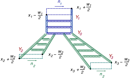
Figure 17: Triple BFKL evolution at $n_{2}=n_{3}$ with BK vertex at the rapidity $Y_{0}$.

$$\big{\langle}{\cal F}^{j_{1}}_{n_{1}}\big{(}x_{1t}+{w_{1t}\over 2},x_{1t}-{w_{1t}\over 2}\big{)}{\cal F}^{j_{2}}_{n_{2}}\big{(}x_{2t}+{w_{2t}\over 2},x_{2t}-{w_{2t}\over 2}\big{)}{\cal F}^{j_{3}}_{n_{2}}\big{(}x_{3t}+{w_{3t}\over 2},x_{3t}-{w_{3t}\over 2}\big{)}\big{\rangle}$$ (146)

As we discussed in Sect. 5.2, this correlator in the Regge limit can be represented by the correlator of three conformal dipoles, one in $n_{1}$ direction and two in $n_{2}$ directions. We get from Eq. (53)

$$\big{\langle}{\cal F}^{j_{1}}_{n_{1}}\big{(}x_{1t}+{w_{1t}\over 2},x_{1t}-{w_{1t}\over 2}\big{)}{\cal F}^{j_{2}}_{n_{2}}\big{(}x_{2t}+{w_{2t}\over 2},x_{2t}-{w_{2t}\over 2}\big{)}{\cal F}^{j_{3}}_{n_{2}}\big{(}x_{3t}+{w_{3t}\over 2},x_{3t}-{w_{3t}\over 2}\big{)}\big{\rangle}$$ (147)

$$=~{}-i{N_{c}^{6}\over\pi^{9}}\!\int_{0}^{\infty}\!{dl_{1}dl_{2}dl_{3}\over l_{1}l_{2}l_{3}}~{}l_{1}^{-\omega_{1}}l_{2}^{-\omega_{2}}l_{3}^{-\omega_{3}}\!\int\!d\nu_{1}d\nu_{2}d\nu_{3}(w_{1t}^{2})^{-{1\over 2}+i\nu_{1}}(w_{2t}^{2})^{-{1\over 2}+i\nu_{2}}(w_{3t}^{2})^{-{1\over 2}+i\nu_{3}}$$

$$\hskip 8.53581pt\times~{}\langle{\cal U}^{Y_{1}}_{\rm conf}(x_{1t},-\nu_{1}){\cal V}^{Y_{2}}_{\rm conf}(x_{2t},-\nu_{2}){\cal V}^{Y_{3}}_{\rm conf}(x_{3t},-\nu_{3})\rangle\prod_{i=1,2,3}\nu_{i}{2^{-4i\nu_{i}}\Gamma\big{(}{3\over 2}+i\nu_{i}\big{)}\Gamma(1-i\nu_{i})\over\Gamma\big{(}{3\over 2}-i\nu_{i}\big{)}\Gamma(1+i\nu_{i})}$$

where $Y_{i}\simeq\ln l_{i}+{1\over 2}\ln sm_{\perp}^{2}$ ($s\equiv s_{12}$).

As discussed in Refs. Balitsky:2015tca and Balitsky:2015oux , the BK equation for color dipoles leads to the following structure of the correlator of a conformal dipole in $n_{1}$ direction and two dipoles in $n_{2}$ direction:

$$\int\!dY_{0}~{}\theta(Y_{0}+Y_{2})\theta(Y_{0}+Y_{3})~{}\big{(}{\rm evolution}~{}{\cal U}^{Y_{1}}\rightarrow{\cal U}^{Y_{0}}\big{)}\otimes({\rm BK~{}vertex~{}at~{}}Y_{0})\otimes\bigg{(}\begin{array}[]{c}\langle{\cal U}^{Y_{0}}{\cal V}^{Y_{2}}\rangle\\ \langle{\cal U}^{Y_{0}}{\cal V}^{Y_{3}}\rangle\end{array}\bigg{)}$$ (148)

where the integral over $Y_{0}$ comes from the fact that the splitting of one dipole into two (described by the BK vertex) can occur at any rapidity between the $n_{1}$ dipole and the most energetic of $n_{2}$ dipoles. Specifically, $\theta(Y_{0}+Y_{i})$ reflects the fact that there should be sufficient energy between dipoles ${\cal U}^{Y_{0}}$ and ${\cal V}^{Y_{i}}$ to apply high-energy approximation, see the footnote 9 at page 14.

Rewrtiting Eq. (18) from Ref. Balitsky:2015tca in terms of conformal dipoles, one gets

$$\langle{\cal U}^{Y_{1}}_{\rm conf}(x_{1t},-\nu_{1}){\cal V}^{Y_{2}}_{\rm conf}(x_{2t},-\nu_{2}){\cal V}^{Y_{3}}_{\rm conf}(x_{3t},-\nu_{3})\rangle~{}=~{}-{\alpha_{s}^{5}N_{c}\over 4\pi^{4}}{1\over\big{(}{1\over 4}+\nu_{2}^{2}\big{)}^{2}\big{(}{1\over 4}+\nu_{3}^{2}\big{)}^{2}}$$

$$\times~{}\!\int_{-\infty}^{Y_{1}}\!dY_{0}\!\int\!dY_{2}dY_{3}~{}\theta(Y_{0}+Y_{2})\theta(Y_{0}+Y_{3})~{}e^{\aleph(\nu_{1})(Y_{1}-Y_{0})+\aleph(\nu_{2})(Y_{0}+Y_{2})+\aleph(\nu_{3})(Y_{0}+Y_{3})}$$

$$\times~{}\!\int\!{d^{2}x_{4}d^{2}x_{5}d^{2}x_{6}\over x_{45}^{2}x_{56}^{2}x_{46}^{2}}\Big{(}{x_{45}^{2}\over x_{14}^{2}x_{15}^{2}}\Big{)}^{{1\over 2}+i\nu_{1}}\Big{(}{x_{56}^{2}\over x_{25}^{2}x_{36}^{2}}\Big{)}^{{1\over 2}+i\nu_{2}}\Big{(}{x_{46}^{2}\over x_{34}^{2}x_{36}^{2}}\Big{)}^{{1\over 2}+i\nu_{3}}~{}+~{}O\big{(}{1\over N_{c}}\big{)}$$ (149)

where two-dimensional integrals go over transverse directions orthogonal to both $n_{1}$ and $n_{2}$. Combining Eqs. (147), (148), and (149) one obtains

$$\big{\langle}{\cal F}^{j_{1}}_{n_{1}}\big{(}x_{1t}+{w_{1t}\over 2},x_{1t}-{w_{1t}\over 2}\big{)}{\cal F}^{j_{2}}_{n_{2}}\big{(}x_{2t}+{w_{2t}\over 2},x_{2t}-{w_{2t}\over 2}\big{)}{\cal F}^{j_{3}}_{n_{2}}\big{(}x_{3t}+{w_{3t}\over 2},x_{3t}-{w_{3t}\over 2}\big{)}\big{\rangle}$$

$$=~{}i{\alpha_{s}^{5}N_{c}^{7}\over 4\pi^{13}}\!\int\!{d\nu_{1}d\nu_{2}d\nu_{3}\over\big{(}{1\over 4}+\nu_{2}^{2}\big{)}^{2}\big{(}{1\over 4}+\nu_{3}^{2}\big{)}^{2}}{2\pi\delta(\omega_{1}-\omega_{2}-\omega_{3})\big{(}{s\over m_{\perp}^{2}}\big{)}^{\omega_{1}+\omega_{2}+\omega_{3}\over 2}\over[\omega_{1}-\aleph(\nu_{1})][\omega_{2}-\aleph(\nu_{2})][\omega_{3}-\aleph(\nu_{3})]}$$

$$\hskip 8.53581pt\times~{}(w_{1t}^{2})^{-{1\over 2}+i\nu_{1}}(w_{2t}^{2})^{-{1\over 2}+i\nu_{2}}(w_{3t}^{2})^{-{1\over 2}+i\nu_{3}}\prod_{k=1,2,3}\nu_{k}{2^{-4i\nu_{k}}\Gamma\big{(}{3\over 2}+i\nu_{k}\big{)}\Gamma(1-i\nu_{k})\over\Gamma\big{(}{3\over 2}-i\nu_{k}\big{)}\Gamma(1+i\nu_{k})}$$

$$\hskip 8.53581pt\times~{}\!\int\!{d^{2}x_{4}d^{2}x_{5}d^{2}x_{6}\over x_{45}^{2}x_{56}^{2}x_{46}^{2}}\Big{(}{x_{45}^{2}\over x_{14}^{2}x_{15}^{2}}\Big{)}^{{1\over 2}+i\nu_{1}}\Big{(}{x_{56}^{2}\over x_{25}^{2}x_{36}^{2}}\Big{)}^{{1\over 2}+i\nu_{2}}\Big{(}{x_{46}^{2}\over x_{34}^{2}x_{36}^{2}}\Big{)}^{{1\over 2}+i\nu_{3}}$$ (150)

Here $2\pi\delta(\omega_{1}-\omega_{2}-\omega_{3})$ comes from the longitudinal integral

$$\int_{0}^{\infty}\!{dl_{1}dl_{2}dl_{3}\over l_{1}l_{2}l_{3}}~{}l_{1}^{-\omega_{1}}l_{2}^{-\omega_{2}}l_{3}^{-\omega_{3}}\!\int_{-\infty}^{Y_{1}}\!dY_{0}\!\int\!dY_{2}dY_{3}~{}\theta(Y_{0}+Y_{2})\theta(Y_{0}+Y_{3})$$

$$\times~{}e^{\aleph(\nu_{1})(Y_{1}-Y_{0})+\aleph(\nu_{2})(Y_{0}+Y_{2})+\aleph(\nu_{3})(Y_{0}+Y_{3})}$$

$$=~{}{2\pi\delta(\omega_{1}-\omega_{2}-\omega_{3})\big{(}{s\over m_{\perp}^{2}}\big{)}^{\omega_{1}+\omega_{2}+\omega_{3}\over 2}\over[\omega_{1}-\aleph(\nu_{1})][\omega_{2}-\aleph(\nu_{2})][\omega_{3}-\aleph(\nu_{3})]}\!\int\!dY_{0}~{}e^{-i(\omega_{1}-\omega_{2}-\omega_{3})Y_{0}}$$

$$\rightarrow~{}{2\pi\delta(\omega_{1}-\omega_{2}-\omega_{3})\big{(}{s\over m_{\perp}^{2}}\big{)}^{\omega_{1}+\omega_{2}+\omega_{3}\over 2}\over[\omega_{1}-\aleph(\nu_{1})][\omega_{2}-\aleph(\nu_{2})][\omega_{3}-\aleph(\nu_{3})]}$$ (151)

Strictly speaking, the integral over $Y_{0}$ is divergent so we need some regularization to understand it. Following Ref. Balitsky:2015tca we take $n_{2}\neq n_{3}$ but $n_{1}\cdot n_{2}\simeq n_{1}\cdot n_{3}$. We can use our formulas for $n_{2}=n_{3}$ case until longitudinal distances between frames “2” and “3” are smaller than typical transverse separation $x_{ij\perp}^{2}\sim m_{\perp}^{-2}$, i.e. when $l_{2}l_{3}s_{23}\leq m_{\perp}^{-2}$. In terms of rapidities $Y_{2}$ and $Y_{3}$ this restriction means $Y_{2}+Y_{3}~{}\leq~{}\ln{s_{12}\over s_{23}}$ so instead of Eq. (151) we get

$$\!\int_{-\infty}^{Y_{1}}\!dY_{0}\!\int\!dY_{2}dY_{3}~{}\theta(Y_{0}+Y_{2})\theta(Y_{0}+Y_{3})\theta\big{(}\ln{s_{12}\over s_{23}}-Y_{2}-Y_{3}\big{)}$$

$$\hskip 31.29802pt\times~{}e^{\aleph(\nu_{1})(Y_{1}-Y_{0})+\aleph(\nu_{2})(Y_{0}+Y_{2})+\aleph(\nu_{3})(Y_{0}+Y_{3})}$$

$$=~{}{\big{(}{s_{23}\over s_{12}}\big{)}^{\omega_{2}+\omega_{3}-\omega_{1}\over 2}\over(\omega_{1}-\omega_{2}-\omega_{3})(\omega_{1}-\aleph_{1})\big{(}\omega_{2}-\aleph_{2}+{\omega_{1}-\omega_{2}-\omega_{3}\over 2}\big{)}\big{(}\omega_{3}-\aleph_{3}+{\omega_{1}-\omega_{2}-\omega_{3}\over 2}\big{)}}$$

$$\hskip 31.29802pt\stackrel{{\scriptstyle\omega_{2}+\omega_{3}\rightarrow\omega_{1}}}{{\rightarrow}}~{}{\big{(}{s_{23}\over s_{12}}\big{)}^{\omega_{2}+\omega_{3}-\omega_{1}\over 2}\over(\omega_{1}-\omega_{2}-\omega_{3})(\omega_{1}-\aleph_{1})(\omega_{2}-\aleph_{2})(\omega_{3}-\aleph_{3})}.$$ (152)

Thus,

$$2\pi\delta(\omega_{1}-\omega_{2}-\omega_{3})~{}\Leftrightarrow~{}\lim_{n_{3}\rightarrow n_{2}}{\big{(}{n_{2}\cdot n_{3}\over n_{1}\cdot n_{2}}\big{)}^{\omega_{2}+\omega_{3}-\omega_{1}\over 2}\over(\omega_{1}-\omega_{2}-\omega_{3})}$$ (153)

Let us emphasize that the divergence over $Y_{0}$ in r.h.s of eq. (152) leading to this $\delta$-function comes from boost invariance: at $n_{2}=n_{3}$ one can multiply $n_{1}$ by some $\lambda$ and $n_{2}$ by $\lambda^{-1}$ and the correlator (147) will not change. Thus, the singularity at $\omega_{1}=\omega_{2}+\omega_{3}$ is of general nature and should be present in a general formula (24). Note, however, that for the correlator of 3 local “forward” operators these singularities seem to disappear, see the discussion in the end of Sect. 8.2.

To compare with the result (111) for $n_{2}\neq n_{3}$ let us finish the calculation in this $n_{2}=n_{3}$ case. The transverse integral was calculated in Ref. Korchemsky:1997fy and the result is

$$\!\int\!{d^{2}x_{4}d^{2}x_{5}d^{2}x_{6}\over x_{45}^{2}x_{56}^{2}x_{46}^{2}}\Big{(}{x_{45}^{2}\over x_{14}^{2}x_{15}^{2}}\Big{)}^{{1\over 2}+i\nu_{1}}\Big{(}{x_{56}^{2}\over x_{25}^{2}x_{36}^{2}}\Big{)}^{{1\over 2}+i\nu_{2}}\Big{(}{x_{46}^{2}\over x_{34}^{2}x_{36}^{2}}\Big{)}^{{1\over 2}+i\nu_{3}}$$

$$=~{}{\pi^{3}\Omega\big{(}{1\over 2}+i\nu_{1},{1\over 2}+i\nu_{2},{1\over 2}+i\nu_{3}\big{)}\over(x_{12}^{2})^{{1\over 2}+i\nu_{1}+i\nu_{2}-i\nu_{3}}(x_{13}^{2})^{{1\over 2}+i\nu_{1}+i\nu_{3}-i\nu_{2}}(x_{23}^{2})^{{1\over 2}+i\nu_{2}+i\nu_{3}-i\nu_{1}}}$$ (154)

where $\Omega$ is related to Meyer G-function, see the explicit expression in Ref. Korchemsky:1997fy (for convenience, we extracted factor $\pi^{3}$ from the definition in Ref. Korchemsky:1997fy ).

Rewriting the intgral (154) in terms of $\gamma_{i}=2i\nu_{i}-1$ one obtains

$$\big{\langle}{\cal F}^{j_{1}}_{n_{1}}\big{(}x_{1t}+{w_{1t}\over 2},x_{1t}-{w_{1t}\over 2}\big{)}{\cal F}^{j_{2}}_{n_{2}}\big{(}x_{2t}+{w_{2t}\over 2},x_{2t}-{w_{2t}\over 2}\big{)}{\cal F}^{j_{3}}_{n_{2}}\big{(}x_{3t}+{w_{3t}\over 2},x_{3t}-{w_{3t}\over 2}\big{)}\big{\rangle}$$

$$\hskip 14.22636pt=~{}-i{\alpha_{s}^{5}N_{c}^{7}\over 64\pi^{10}}{2\pi\delta(\omega_{1}-\omega_{2}-\omega_{3})\over x_{12t}^{2}x_{13t}^{2}x_{23t}^{2}}\!\int_{-1-i\infty}^{-1+i\infty}\!{d\gamma_{1}d\gamma_{2}d\gamma_{3}\over\gamma_{2}^{2}\gamma_{3}^{2}(2+\gamma_{2})^{2}(2+\gamma_{3})^{2}}$$

$$\hskip 31.29802pt\times~{}\prod_{k=1}^{3}{(1+\gamma_{k})2^{-2\gamma_{k}}\Gamma\big{(}2+{\gamma_{k}\over 2}\big{)}\Gamma\big{(}{1\over 2}-{\gamma_{k}\over 2}\big{)}\over\Gamma\big{(}1-{\gamma_{k}\over 2}\big{)}\Gamma\big{(}{3\over 2}+{\gamma_{k}\over 2}\big{)}}{\Omega\big{(}1-{\gamma_{1}\over 2},1-{\gamma_{2}\over 2},1-{\gamma_{3}\over 2}\big{)}\over[\omega_{1}-\tilde{\aleph}(\gamma_{1})][\omega_{2}-\tilde{\aleph}(\gamma_{2})][\omega_{3}-\tilde{\aleph}(\gamma_{3})]}$$

$$\hskip 31.29802pt\times~{}\Big{(}{w_{1t}^{2}x_{23t}^{2}\over x_{12t}^{2}x_{13t}^{2}}\Big{)}^{\gamma_{1}\over 2}\Big{(}{w_{2t}^{2}x_{13t}^{2}\over x_{12t}^{2}x_{23t}^{2}}\Big{)}^{\gamma_{2}\over 2}\Big{(}{w_{3t}^{2}x_{12t}^{2}\over x_{13t}^{2}x_{23t}^{2}}\Big{)}^{\gamma_{3}\over 2}\big{(}{s\over m_{\perp}^{2}}\big{)}^{\omega_{1}+\omega_{2}+\omega_{3}\over 2}$$ (155)

where $\gamma_{i}=2i\nu_{i}-1$ similarly to Eq. (106).

Taking residues at $\gamma^{\ast}_{i}$ (roots of the equation (110)) one obtains

$$\big{\langle}{\cal F}^{j_{1}}_{n_{1}}\big{(}x_{1t}+{w_{1t}\over 2},x_{1t}-{w_{1t}\over 2}\big{)}{\cal F}^{j_{2}}_{n_{2}}\big{(}x_{2t}+{w_{2t}\over 2},x_{2t}-{w_{2t}\over 2}\big{)}{\cal F}^{j_{3}}_{n_{2}}\big{(}x_{3t}+{w_{3t}\over 2},x_{3t}-{w_{3t}\over 2}\big{)}\big{\rangle}$$

$$=~{}8g^{10}{N_{c}^{2}\over\pi^{2}}2\pi\delta(\omega_{1}-\omega_{2}-\omega_{3})\big{(}{s\over x_{12t}^{2}}\big{)}^{\omega_{1}+\omega_{2}-\omega_{3}\over 2}\big{(}{s\over x_{13t}^{2}}\big{)}^{\omega_{1}+\omega_{3}-\omega_{2}\over 2}\big{(}{s\over x_{23t}^{2}}\big{)}^{\omega_{2}+\omega_{3}-\omega_{1}\over 2}$$

$$\times~{}\Omega\big{(}1-{\gamma^{\ast}_{1}\over 2},1-{\gamma^{\ast}_{2}\over 2},1-{\gamma^{\ast}_{3}\over 2}\big{)}{1\over x_{12t}^{2}x_{13t}^{2}x_{23t}^{2}}\Big{(}{w_{1t}^{2}x_{23t}^{2}\over x_{12t}^{2}x_{13t}^{2}}\Big{)}^{\gamma^{\ast}_{1}\over 2}\Big{(}{w_{2t}^{2}x_{13t}^{2}\over x_{12t}^{2}x_{23t}^{2}}\Big{)}^{\gamma^{\ast}_{2}\over 2}\Big{(}{w_{3t}^{2}x_{12t}^{2}\over x_{13t}^{2}x_{23t}^{2}}\Big{)}^{\gamma^{\ast}_{3}\over 2}$$

$$\times~{}{1\over{\gamma_{2}^{\ast}}^{2}{\gamma_{3}^{\ast}}^{2}\big{(}1+{\gamma^{\ast}_{2}\over 2}\big{)}^{2}\big{(}1+{\gamma_{3}^{\ast}\over 2}\big{)}^{2}}\prod_{k=1}^{3}{(1+\gamma^{\ast}_{k})2^{-2\gamma^{\ast}_{k}}\Gamma\big{(}2+{\gamma^{\ast}_{k}\over 2}\big{)}\Gamma\big{(}{1\over 2}-{\gamma^{\ast}_{k}\over 2}\big{)}\over\Gamma\big{(}1-{\gamma^{\ast}_{k}\over 2}\big{)}\Gamma\big{(}{3\over 2}+{\gamma^{\ast}_{k}\over 2}\big{)}\aleph^{\prime}(\gamma^{\ast}_{k})}$$ (156)

Here again we replaced $\big{(}{s\over m_{\perp}^{2}})^{\omega_{1}+\omega_{2}+\omega_{3}\over 2}$ by $\big{(}{s\over x_{12t}^{2}}\big{)}^{\omega_{1}+\omega_{2}-\omega_{3}\over 2}\big{(}{s\over x_{13t}^{2}}\big{)}^{\omega_{1}+\omega_{3}-\omega_{2}\over 2}\big{(}{s\over x_{23t}^{2}}\big{)}^{\omega_{2}+\omega_{3}-\omega_{1}\over 2}$ which is within LLA accuracy. This result agrees with Eq. (30) from Ref. Balitsky:2015tca . In terms of structure constant (24) we have

$$F\big{[}\gamma^{\ast}(\omega_{1},g^{2}),\gamma^{\ast}(\omega_{2},g^{2}),\gamma^{\ast}(\omega_{3},g^{2})\big{]}$$ (157)

$$\stackrel{{\scriptstyle\omega_{1}=\omega_{2}+\omega_{3}}}{{=}}8ig^{10}{N_{c}^{2}\over\pi^{2}}{\Omega\big{(}1-{\gamma^{\ast}_{1}\over 2},1-{\gamma^{\ast}_{2}\over 2},1-{\gamma^{\ast}_{3}\over 2}\big{)}\over{\gamma_{2}^{\ast}}^{2}{\gamma_{3}^{\ast}}^{2}\big{(}1+{\gamma^{\ast}_{2}\over 2}\big{)}^{2}\big{(}1+{\gamma_{3}^{\ast}\over 2}\big{)}^{2}}\prod_{k=1}^{3}{(1+\gamma^{\ast}_{k})2^{-2\gamma^{\ast}_{k}}\Gamma\big{(}2+{\gamma^{\ast}_{k}\over 2}\big{)}\Gamma\big{(}{1\over 2}-{\gamma^{\ast}_{k}\over 2}\big{)}\over\Gamma\big{(}1-{\gamma^{\ast}_{k}\over 2}\big{)}\Gamma\big{(}{3\over 2}+{\gamma^{\ast}_{k}\over 2}\big{)}\aleph^{\prime}(\gamma^{\ast}_{k})}$$

It is instructive to compare with the result (111) at small $\gamma^{\ast}_{i}\simeq-{8g^{2}\over\omega_{i}}\ll 1$. The estimate of the function $\Omega$ at small $\gamma_{i}$ reads Balitsky:2015tca ; Balitsky:2015oux

$$\Omega\big{(}1-{\gamma_{1}\over 2},1-{\gamma_{2}\over 2},1-{\gamma_{3}\over 2}\big{)}~{}=~{}{16\over\gamma_{1}\gamma_{2}\gamma_{3}}\big{(}1+{\gamma_{1}+\gamma_{2}\over\gamma_{3}}+{\gamma_{1}+\gamma_{3}\over\gamma_{2}}+{\gamma_{2}+\gamma_{3}\over\gamma_{1}}\big{)}~{}+~{}O(\gamma_{i})$$ (158)

so we get

$$\big{\langle}{\cal F}^{j_{1}}_{n_{1}}\big{(}x_{1t}+{w_{1t}\over 2},x_{1t}-{w_{1t}\over 2}\big{)}{\cal F}^{j_{2}}_{n_{2}}\big{(}x_{2t}+{w_{2t}\over 2},x_{2t}-{w_{2t}\over 2}\big{)}{\cal F}^{j_{3}}_{n_{2}}\big{(}x_{3t}+{w_{3t}\over 2},x_{3t}-{w_{3t}\over 2}\big{)}\big{\rangle}$$ (159)

$$=~{}-{g^{2}N_{c}^{2}\over 2\pi^{2}}\omega_{1}[2\pi\delta(\omega_{1}-\omega_{2}-\omega_{3})]\Big{(}{w_{1t}^{2}x_{23t}^{2}\over x_{12t}^{2}x_{13t}^{2}}\Big{)}^{\gamma^{\ast}_{1}\over 2}\Big{(}{w_{2t}^{2}x_{13t}^{2}\over x_{12t}^{2}x_{23t}^{2}}\Big{)}^{\gamma^{\ast}_{2}\over 2}\Big{(}{w_{3t}^{2}x_{12t}^{2}\over x_{13t}^{2}x_{23t}^{2}}\Big{)}^{\gamma^{\ast}_{3}\over 2}\big{[}1+O\big{(}{g^{2}\over\omega}\big{)}\big{]}$$

which corresponds to structure constant (24) with

$$F~{}=~{}-2i\pi g^{2}$$

at $\omega_{1}=\omega_{2}+\omega_{3}$. This contribution to structure constant is imaginary in accordance with the fact that the physical amplitude in Fig. (17) is purely imaginary if left and right sides are symmetric. (The corresponding cross section describes diffractive scattering, see Refs. Balitsky:1997mk ; Balitsky:2001gj ). Since the leading-order structure constant (114) is real, it is natural to assume that Eq. (157) gives the leading contribution to the imaginary part of structure constant at $\omega_{1}=\omega_{2}+\omega_{3}$ in the BFKL limit.

8.4 Calculation of $\Lambda(\nu_{1},\nu_{2},\nu_{3})$

The function $\Lambda(\nu_{1},\nu_{2},\nu_{3})$ is represented by the integral (102). It is convenient to take $x=(1,0)$ and rewrite the integral as

$$\Lambda(\nu_{1},\nu_{2},\nu_{3})~{}\equiv~{}{\bar{\Lambda}}(\epsilon_{1},\epsilon_{2},\epsilon_{3})~{}=~{}{1\over\pi^{3}}\!\int\!d^{2}z_{1}{d^{2}z_{2}\over(1-z_{2})^{4}}{d^{2}z_{0}\over z_{0}^{4}}$$

$$\times~{}[z_{12x}^{2}+(z_{1y}+z_{2y})^{2}]^{-\epsilon_{1}}\Big{[}{z_{20}^{2}\over(1-z_{2})^{2}(1-z_{0})^{2}}\Big{]}^{-\epsilon_{2}}\Big{[}{z_{10}^{2}\over z_{1}^{2}z_{0}^{2}}\Big{]}^{-\epsilon_{3}}$$ (160)

where we denote $\epsilon_{i}\equiv{1\over 2}-i\nu_{i}$ in a view of a later estimate at $\epsilon_{i}\rightarrow 0$. Unfortunately, the integral (160) diverges as $\epsilon_{i}\rightarrow 0$ so we need to define it as an analytic continuation of a convergent integral

$${\bar{\Lambda}}^{a}(\epsilon_{1},\epsilon_{2},\epsilon_{3})~{}\equiv~{}{1\over\pi^{3}}\!\int\!d^{2}z_{0}d^{2}z_{1}d^{2}z_{2}{1\over(|1-z_{0}|^{2})^{a-\epsilon_{2}}(|1-z_{2}|^{2})^{2-a-\epsilon_{2}}}$$

$$\times~{}({\bar{z}}_{2}-z_{1})^{-\epsilon_{1}}(z_{2}-{\bar{z}}_{1})^{-\epsilon_{1}}{1\over|z_{20}^{2}|^{\epsilon_{2}}|z_{1}^{2}|^{a-\epsilon_{3}}|z_{10}^{2}|^{\epsilon_{3}}|z_{0}^{2}|^{2-a-\epsilon_{3}}}$$ (161)

This integral is obviously convergent if $\epsilon_{i}>0$ and $|1-a|<\epsilon_{i}$. (We will relax the condition $\epsilon_{i}>0$ later). The “Feynman diagram” integral is depicted in Fig. 18

Figure 18: Correlator defining the function $\Lambda(\epsilon_{i})$ ($\equiv\Lambda(e_{i})$) in Eq. (160). Dotted line depicts the unusial propagator $[z_{12x}^{2}+(z_{1y}+z_{2y})^{2}]^{-e_{1}}$ between points $z_{1}$ and $z_{2}$.

the denominators being conventional 2-dim propagators (albeit with non-integer powers) except $[z_{12x}^{2}+(z_{1y}+z_{2y})^{2}]^{-\epsilon_{1}}$ denoted by a dotted line.

To calculate this integral, we will rewrite $[z_{12x}^{2}+(z_{1y}+z_{2y})^{2}]$ in the denominator as $({\bar{z}}_{2}-z_{1})(z_{2}-{\bar{z}}_{1})$ where $z\equiv z_{x}+iz_{y},~{}{\bar{z}}\equiv z_{x}-iz_{y}$ and use the expansion

$${1\over({\bar{z}}_{2}-z_{1})^{\epsilon_{1}}(z_{2}-{\bar{z}}_{1})^{\epsilon_{1}}}~{}=~{}\sum_{m,n=0}^{\infty}{\Gamma(\epsilon_{1}+m+n)\over\Gamma(\epsilon_{1})m!n!}(1-{\bar{z}}_{2})^{m}z_{1}^{n}\sum_{k,l=0}^{\infty}{\Gamma(\epsilon_{1}+k+l)\over\Gamma(a)k!l!}(1-z_{2})^{k}{\bar{z}}_{1}^{l}$$ (162)

Next, we use the expansion (162), calculate the integrals, reassemble the sum over $m,n,k,l$ and continue analytically to $a=0$ in the final result.

Using the integral

$$\int\!{d^{2}z_{1}\over\pi}{z_{1}^{m}{\bar{z}}_{1}^{n}\over|z_{2}-z_{1}|^{2\alpha}|z_{1}|^{2\beta}}~{}=~{}{\Gamma(\alpha+\beta-n-1)\over\Gamma(\alpha)\Gamma(\beta-n)|z_{2}^{2}|^{\alpha+\beta-n-1}}z_{2}^{m-n}{\Gamma(1-\alpha)\Gamma(1-\beta+m)\over\Gamma(2-\alpha-\beta+m)}$$ (163)

one obtains after some algebra

$${\bar{\Lambda}}^{a}(\epsilon_{1},\epsilon_{2},\epsilon_{3})~{}$$

$$=~{}{\sin\pi(a+\epsilon_{2})\sin\pi\epsilon_{2}\sin\pi(\epsilon_{3}-a)\sin\pi\epsilon_{3}\over\pi^{3}\sin\pi(\epsilon_{2}+\epsilon_{3})}\!\!\sum_{m,n,k,l=0}^{\infty}{\Gamma(\epsilon_{1}+m+n)\over\Gamma(\epsilon_{1})m!n!}{\Gamma(\epsilon_{1}+k+l)\over\Gamma(\epsilon_{1})k!l!}$$

$$\times~{}(-1)^{m+l}{\Gamma(a+\epsilon_{2}-1+m)\Gamma(1-a-m)\over\Gamma(\epsilon_{2})}{\Gamma(1-\epsilon_{2})\Gamma(\epsilon_{2}+a-1+k)\over\Gamma(a+k)}$$

$$\times~{}{\Gamma(\epsilon_{3}+l+1-a)\Gamma(a-l-1)\over\Gamma(\epsilon_{3})}{\Gamma(1-\epsilon_{3})\Gamma(1+\epsilon_{3}-a+n)\over\Gamma(2-a+n)}$$

$$\times~{}{\Gamma(\epsilon_{2}+m)\Gamma(\epsilon_{3}+l)\over\Gamma(\epsilon_{2}+\epsilon_{3}+m+l)}{\Gamma(\epsilon_{2}+k)\Gamma(\epsilon_{3}+n)\over\Gamma(\epsilon_{2}+\epsilon_{3}+k+n)}$$

$$=~{}-{\sin\pi(a+\epsilon_{2})\sin\pi\epsilon_{2}\sin\pi(\epsilon_{3}-a)\sin\pi\epsilon_{3}\over\pi^{3}\sin\pi(\epsilon_{2}+\epsilon_{3})}\sum_{m,n=0}^{\infty}{\Gamma(\epsilon_{1}+m+n)\over\Gamma(\epsilon_{1})m!n!}\sum_{k,l=0}^{\infty}{\Gamma(\epsilon_{1}+k+l)\over\Gamma(\epsilon_{1})k!l!}$$

$$\times~{}(-1)^{m+l}\!\int_{0}^{1}\!du_{1}dv_{1}du_{2}dv_{2}dt_{1}dt_{2}~{}u_{1}^{a+\epsilon_{2}-2+m}(1-u_{1})^{-a-m}(1-v_{1})^{-\epsilon_{2}}v_{1}^{\epsilon_{2}+a-2+k}u_{2}^{\epsilon_{3}-a+l}$$

$$\times~{}(1-u_{2})^{a-2-l}(1-v_{2})^{-\epsilon_{3}}v_{2}^{\epsilon_{3}-a+n}t_{1}^{\epsilon_{2}-1+m}(1-t_{1})^{\epsilon_{3}-1+l}t_{2}^{\epsilon_{2}-1+k}(1-t_{2})^{\epsilon_{3}-1+n}$$ (164)

Now one can reassemble the sum (162) and get

$${\bar{\Lambda}}^{a}(\epsilon_{1},\epsilon_{2},\epsilon_{3})~{}=~{}-{\sin\pi(a+\epsilon_{2})\sin\pi\epsilon_{2}\sin\pi(\epsilon_{3}-a)\sin\pi\epsilon_{3}\over\pi^{3}\sin\pi(\epsilon_{2}+\epsilon_{3})}\int_{0}^{1}\!du_{1}dv_{1}du_{2}dv_{2}dt_{1}dt_{2}~{}$$

$$\times~{}u_{1}^{a+\epsilon_{2}-2}(1-u_{1})^{\epsilon_{1}-a}(1-v_{1})^{-\epsilon_{2}}v_{1}^{\epsilon_{2}+a-2}u_{2}^{\epsilon_{3}-a}(1-u_{2})^{\epsilon_{1}+a-2}(1-v_{2})^{-\epsilon_{3}}v_{2}^{\epsilon_{3}-a}$$

$$\times~{}t_{1}^{\epsilon_{2}-1}(1-t_{1})^{\epsilon_{3}-1}t_{2}^{\epsilon_{2}-1}(1-t_{2})^{\epsilon_{3}-1}\big{[}(1-u_{1})(1-v_{2})+u_{1}t_{1}+(1-u_{1})v_{2}t_{2}\big{]}^{-\epsilon_{1}}$$

$$\hskip 31.29802pt\times~{}\big{[}(1-u_{2})(1-v_{1})+u_{2}(1-t_{1})+(1-u_{2})v_{1}(1-t_{2})\big{]}^{-\epsilon_{1}}$$ (165)

Next, using Mellin-Barnes integral

$${\Gamma(a)\over(A+B+C)^{a}}~{}=~{}{1\over(2\pi i)^{2}}\!\int\!ds_{1}ds_{2}~{}{\Gamma(a-s_{1})\over A^{a-s_{1}}}{\Gamma(s_{1}-s_{2})\over B^{s_{1}-s_{2}}}{\Gamma(s_{2})\over C^{s_{2}}}$$ (166)

one can rewrite Eq. (165) as follows

$${\bar{\Lambda}}^{a}(\epsilon_{1},\epsilon_{2},\epsilon_{3})~{}=~{}-{\sin\pi(a+\epsilon_{2})\sin\pi(\epsilon_{2})\sin\pi(\epsilon_{3}-a)\sin\pi(\epsilon_{3})\over\pi^{3}\sin\pi(\epsilon_{2}+\epsilon_{3})\Gamma^{2}(\epsilon_{1})}I^{a}(\epsilon_{1},\epsilon_{2},\epsilon_{3})$$ (167)

where $I^{a}(\epsilon_{1},\epsilon_{2},\epsilon_{3})=I^{a,a,a,a}(\epsilon_{1},\epsilon_{2},\epsilon_{3})$ and

$$I^{a_{1},a_{2},a_{3},a_{4}}(\epsilon_{1},\epsilon_{2},\epsilon_{3})~{}$$ (168)

$$=~{}\!\int_{\delta-i\infty}^{\delta+i\infty}\!{ds_{1}ds_{2}ds_{3}ds_{4}\over(2\pi i)^{4}}~{}\Gamma(\epsilon_{1}-s_{1}-s_{2})\Gamma(s_{1})\Gamma(s_{2})\Gamma(\epsilon_{1}-s_{3}-s_{4})\Gamma(s_{3})\Gamma(s_{4})$$

$$\times~{}{\Gamma(\epsilon_{2}-1+a_{3}-s_{1})\Gamma(s_{1}-a_{3}+1)\over\Gamma(\epsilon_{2})}~{}{\Gamma(1+\epsilon_{3}-a_{1}-s_{3})\Gamma(a_{1}-1+s_{3})\over\Gamma(\epsilon_{3})}~{}$$

$$\times~{}{\Gamma(\epsilon_{2}-1+a_{2}-s_{4})\Gamma(1-\epsilon_{1}-\epsilon_{2}+s_{3}+s_{4})\over\Gamma(a_{2}-\epsilon_{1}+s_{3})}$$

$$\times~{}{\Gamma(1+\epsilon_{3}-a_{4}-s_{2})\Gamma(1-\epsilon_{1}-\epsilon_{3}+s_{1}+s_{2})\over\Gamma(2-a_{4}-\epsilon_{1}+s_{1})}{\Gamma(\epsilon_{2}-s_{1})\Gamma(\epsilon_{3}-s_{3})\over\Gamma(\epsilon_{2}+\epsilon_{3}-s_{1}-s_{3})}{\Gamma(\epsilon_{2}-s_{2})\Gamma(\epsilon_{3}-s_{4})\over\Gamma(\epsilon_{2}+\epsilon_{3}-s_{2}-s_{4})}$$

Here we assume $|1-a_{i}|<\delta<{\epsilon_{i}\over 2}$, then the MB integral is well-defined with all the “left” poles of the type $\Gamma(s_{i}+...)$ to the left of the contour of integration over $s_{i}$ and “right” poles $\sim\Gamma(...-s_{i})$ to the right of the contour.

Next, we need to continue analytically to $a_{i}=0$. We will do this separately for each $a_{i}$ paying attention to the poles which intersect the contour of integration and taking residues in those poles as explained in the book Smirnov:2006ry . First, note that analytic continuation in $a_{4}$ is trivial: “right” pole at $s_{2}=1+\epsilon_{3}-a_{4}$ moves to the right and away from the contour. Thus, we set $a_{4}=0$ in what follows. At a next step, we continue $a_{1}$ to $a_{1}=0$. There are two poles affected by that: pole at $s_{3}=1+\epsilon_{3}-a_{1}$ and pole at $s_{3}=1-a_{1}$. While the first pole is always to the right of the contour, the second pole intersects the contour so we need to take a residue at $s_{3}=1-a_{1}$. The integral $I^{a_{1},a_{2},a_{3},0}$ at $a_{1}\leq 1-\delta$ takes the form

$$I^{a_{1},a_{2},a_{3},0}~{}=~{}{\rm r.h.s.~{}of~{}Eq.(\ref{begin})}\Big{|}_{a_{1}=a_{4}=0}$$

$$+~{}\Gamma(1-a_{1})\!\int_{\delta-i\infty}^{\delta+i\infty}\!{ds_{1}ds_{2}ds_{4}\over(2\pi i)^{3}}\Gamma(\epsilon_{1}-s_{1}-s_{2})\Gamma(s_{1})\Gamma(s_{2})\Gamma(a_{1}+\epsilon_{1}-1-s_{4})\Gamma(s_{4})$$ (169)

$$\times~{}{\Gamma(\epsilon_{2}-1+a_{3}-s_{1})\Gamma(s_{1}-a_{3}+1)\over\Gamma(\epsilon_{2})}{\Gamma(\epsilon_{2}-1+a_{2}-s_{4})\Gamma(2-a_{1}-\epsilon_{1}-\epsilon_{2}+s_{4})\over\Gamma(1-a_{1}+a_{2}-\epsilon_{1})}$$

$$\times~{}{\Gamma(1+\epsilon_{3}-s_{2})\Gamma(1-\epsilon_{1}-\epsilon_{3}+s_{1}+s_{2})\over\Gamma(2-\epsilon_{1}+s_{1})}{\Gamma(\epsilon_{2}-s_{1})\Gamma(a_{1}+\epsilon_{3}-1)\over\Gamma(a_{1}+\epsilon_{2}+\epsilon_{3}-s_{1}-1)}{\Gamma(\epsilon_{2}-s_{2})\Gamma(\epsilon_{3}-s_{4})\over\Gamma(\epsilon_{2}+\epsilon_{3}-s_{2}-s_{4})}$$

Now we should continue from $a_{1}=1-\delta$ to $a_{1}=0$. In the first term in r.h.s. of Eq. (169) there are no more crossings of the contour so we can just set $a_{1}=0$. In the second term, the pole at $s_{4}=a_{1}+\epsilon_{1}+\epsilon_{2}-2$ will always stay to the left of the cut but the pole at $s_{4}=a_{1}+\epsilon_{1}-1$ will move from $s_{4}=\epsilon_{1}-\delta$ to $s_{4}=\epsilon_{1}-1$ so it will cross the contour and we need to take the residue. The residue yields

$$\Gamma(1-a_{1})\!\int_{\delta-i\infty}^{\delta+i\infty}\!{ds_{1}ds_{2}\over(2\pi i)^{2}}\Gamma(\epsilon_{1}-s_{1}-s_{2})\Gamma(s_{1})\Gamma(s_{2})\Gamma(a_{1}+\epsilon_{1}-1)$$ (170)

$$\hskip 31.29802pt\times~{}{\Gamma(\epsilon_{2}-1+a_{3}-s_{1})\Gamma(s_{1}-a_{3}+1)\over\Gamma(\epsilon_{2})}{\Gamma(\epsilon_{2}-\epsilon_{1}+a_{2}-a_{1})\Gamma(2-a_{1}-\epsilon_{1}-\epsilon_{2}+s_{4})\over\Gamma(1-a_{1}+a_{2}-\epsilon_{1})}$$

$$\hskip 31.29802pt\times~{}{\Gamma(1+\epsilon_{3}-s_{2})\Gamma(1-\epsilon_{1}-\epsilon_{3}+s_{1}+s_{2})\over\Gamma(2-\epsilon_{1}+s_{1})}{\Gamma(\epsilon_{2}-s_{1})\Gamma(a_{1}+\epsilon_{3}-1)\over\Gamma(a_{1}+\epsilon_{2}+\epsilon_{3}-s_{1}-1)}$$

$$\hskip 219.08621pt\times~{}{\Gamma(\epsilon_{2}-s_{2})\Gamma(1-\epsilon_{1}-\epsilon_{3}-a_{1})\over\Gamma(1+\epsilon_{2}+\epsilon_{3}-\epsilon_{1}-s_{2}-a_{1})}$$

The continuation $a_{1}\rightarrow 0$ in Eq. (170) does not cross the integration contours so we can set $a_{1}=0$ and get for Eq. (168)

$$I^{a_{1}\rightarrow 0,a_{2},a_{3},0}(\epsilon_{1},\epsilon_{2},\epsilon_{3})~{}$$ (171)

$$=~{}\!\int_{\delta-i\infty}^{\delta+i\infty}\!{ds_{1}ds_{2}ds_{3}ds_{4}\over(2\pi i)^{4}}~{}\Gamma(\epsilon_{1}-s_{1}-s_{2})\Gamma(s_{1})\Gamma(s_{2})\Gamma(\epsilon_{1}-s_{3}-s_{4})\Gamma(s_{3})\Gamma(s_{4})$$

$$\times~{}{\Gamma(\epsilon_{2}-1+a_{3}-s_{1})\Gamma(s_{1}-a_{3}+1)\over\Gamma(\epsilon_{2})}~{}{\Gamma(1+\epsilon_{3}-s_{3})\Gamma(s_{3}-1)\over\Gamma(\epsilon_{3})}~{}$$

$$\times~{}{\Gamma(\epsilon_{2}-1+a_{2}-s_{4})\Gamma(1-\epsilon_{1}-\epsilon_{2}+s_{3}+s_{4})\over\Gamma(a_{2}-\epsilon_{1}+s_{3})}$$

$$\times~{}{\Gamma(1+\epsilon_{3}-s_{2})\Gamma(1-\epsilon_{1}-\epsilon_{3}+s_{1}+s_{2})\over\Gamma(2-\epsilon_{1}+s_{1})}{\Gamma(\epsilon_{2}-s_{1})\Gamma(\epsilon_{3}-s_{3})\over\Gamma(\epsilon_{2}+\epsilon_{3}-s_{1}-s_{3})}{\Gamma(\epsilon_{2}-s_{2})\Gamma(\epsilon_{3}-s_{4})\over\Gamma(\epsilon_{2}+\epsilon_{3}-s_{2}-s_{4})}$$

$$+~{}\!\int_{\delta-i\infty}^{\delta+i\infty}\!{ds_{1}ds_{2}ds_{4}\over(2\pi i)^{3}}\Gamma(\epsilon_{1}-s_{1}-s_{2})\Gamma(s_{1})\Gamma(s_{2})\Gamma(\epsilon_{1}-1-s_{4})\Gamma(s_{4})$$

$$\times~{}{\Gamma(\epsilon_{2}-1+a_{3}-s_{1})\Gamma(s_{1}-a_{3}+1)\over\Gamma(\epsilon_{2})}{\Gamma(\epsilon_{2}-1+a_{2}-s_{4})\Gamma(2-\epsilon_{1}-\epsilon_{2}+s_{4})\over\Gamma(1+a_{2}-\epsilon_{1})}$$

$$\times~{}{\Gamma(1+\epsilon_{3}-s_{2})\Gamma(1-\epsilon_{1}-\epsilon_{3}+s_{1}+s_{2})\over\Gamma(2-\epsilon_{1}+s_{1})}{\Gamma(\epsilon_{2}-s_{1})\Gamma(\epsilon_{3}-1)\over\Gamma(\epsilon_{2}+\epsilon_{3}-s_{1}-1)}{\Gamma(\epsilon_{2}-s_{2})\Gamma(\epsilon_{3}-s_{4})\over\Gamma(\epsilon_{2}+\epsilon_{3}-s_{2}-s_{4})}$$

$$+~{}\!\int_{\delta-i\infty}^{\delta+i\infty}\!{ds_{1}ds_{2}\over(2\pi i)^{2}}\Gamma(\epsilon_{1}-s_{1}-s_{2})\Gamma(s_{1})\Gamma(s_{2})\Gamma(\epsilon_{1}-1)$$

$$\times~{}{\Gamma(\epsilon_{2}-1+a_{3}-s_{1})\Gamma(s_{1}-a_{3}+1)\over\Gamma(\epsilon_{2})}{\Gamma(\epsilon_{2}-\epsilon_{1}+a_{2})\Gamma(2-\epsilon_{1}-\epsilon_{2}+s_{4})\over\Gamma(1+a_{2}-\epsilon_{1})}$$

$$\times~{}{\Gamma(1+\epsilon_{3}-s_{2})\Gamma(1-\epsilon_{1}-\epsilon_{3}+s_{1}+s_{2})\over\Gamma(2-\epsilon_{1}+s_{1})}{\Gamma(\epsilon_{2}-s_{1})\Gamma(\epsilon_{3}-1)\over\Gamma(\epsilon_{2}+\epsilon_{3}-s_{1}-1)}{\Gamma(\epsilon_{2}-s_{2})\Gamma(1-\epsilon_{1}-\epsilon_{3})\over\Gamma(1+\epsilon_{2}+\epsilon_{3}-\epsilon_{1}-s_{2})}$$

Repeating this procedure for $a_{2}$ and $a_{3}$ one obtains after some algebra

$${\bar{\Lambda}}(\epsilon_{1},\epsilon_{2},\epsilon_{3})~{}=~{}-{\sin^{2}\pi\epsilon_{2}\sin^{2}\pi\epsilon_{3}\over\pi^{3}\sin\pi(\epsilon_{2}+\epsilon_{3})\Gamma^{2}(\epsilon_{1})}I^{a_{1}\rightarrow 0,a_{2}\rightarrow 0,a_{3}\rightarrow 0,0}(\epsilon_{1},\epsilon_{2},\epsilon_{3})$$ (172)

$$I^{a_{1}\rightarrow 0,a_{2}\rightarrow 0,a_{3}\rightarrow 0,0}(\epsilon_{1},\epsilon_{2},\epsilon_{3})~{}=~{}J_{1}(\epsilon_{i})+J_{2}(\epsilon_{i})+...+J_{14}(\epsilon_{i})$$ (173)

where

$$J_{1}~{}=~{}\!\int_{\delta-i\infty}^{\delta+i\infty}\!{ds_{1}ds_{2}ds_{3}ds_{4}\over(2\pi i)^{4}}~{}\Gamma(\epsilon_{1}-s_{1}-s_{2})\Gamma(s_{1})\Gamma(s_{2})\Gamma(\epsilon_{1}-s_{3}-s_{4})\Gamma(s_{3})\Gamma(s_{4})$$

$$\times~{}{\Gamma(\epsilon_{2}-1-s_{1})\Gamma(s_{1}+1)\over\Gamma(\epsilon_{2})}~{}{\Gamma(1+\epsilon_{3}-s_{3})\Gamma(s_{3}-1)\over\Gamma(\epsilon_{3})}~{}{\Gamma(\epsilon_{2}-1-s_{4})\Gamma(1-\epsilon_{1}-\epsilon_{2}+s_{3}+s_{4})\over\Gamma(-\epsilon_{1}+s_{3})}$$

$$\times~{}{\Gamma(1+\epsilon_{3}-s_{2})\Gamma(1-\epsilon_{1}-\epsilon_{3}+s_{1}+s_{2})\over\Gamma(2-\epsilon_{1}+s_{1})}{\Gamma(\epsilon_{2}-s_{1})\Gamma(\epsilon_{3}-s_{3})\over\Gamma(\epsilon_{2}+\epsilon_{3}-s_{1}-s_{3})}{\Gamma(\epsilon_{2}-s_{2})\Gamma(\epsilon_{3}-s_{4})\over\Gamma(\epsilon_{2}+\epsilon_{3}-s_{2}-s_{4})}$$ (174)

$$J_{2}~{}=~{}{\Gamma(\epsilon_{2}-1)\Gamma(1+\epsilon_{3}-\epsilon_{2})\over\Gamma(\epsilon_{2})\Gamma(\epsilon_{3})}\!\int_{\delta-i\infty}^{\delta+i\infty}\!{ds_{1}ds_{2}ds_{3}\over(2\pi i)^{3}}~{}\Gamma(\epsilon_{1}-s_{1}-s_{2})\Gamma(s_{1})\Gamma(s_{2})$$

$$\times~{}\Gamma(1+\epsilon_{1}-\epsilon_{2}-s_{3})\Gamma(s_{3})\Gamma(\epsilon_{2}-1-s_{1})\Gamma(s_{1}+1)\Gamma(1+\epsilon_{3}-s_{3})\Gamma(s_{3}-1)$$ (175)

$$\times~{}{\Gamma(1+\epsilon_{3}-s_{2})\Gamma(1-\epsilon_{1}-\epsilon_{3}+s_{1}+s_{2})\over\Gamma(2-\epsilon_{1}+s_{1})}{\Gamma(\epsilon_{2}-s_{1})\Gamma(\epsilon_{3}-s_{3})\over\Gamma(\epsilon_{2}+\epsilon_{3}-s_{1}-s_{3})}{\Gamma(\epsilon_{2}-s_{2})\over\Gamma(1+\epsilon_{3}-s_{2})}$$

$$J_{3}~{}=~{}{\Gamma(\epsilon_{3}-1)\over\Gamma(\epsilon_{2})}\!\int_{\delta-i\infty}^{\delta+i\infty}\!{ds_{1}ds_{2}ds_{4}\over(2\pi i)^{3}}~{}\Gamma(\epsilon_{1}-s_{1}-s_{2})\Gamma(s_{1})\Gamma(s_{2})\Gamma(\epsilon_{1}-1-s_{4})\Gamma(s_{4})$$

$$\times~{}\Gamma(\epsilon_{2}-1-s_{1})\Gamma(s_{1}+1)~{}{\Gamma(\epsilon_{2}-1-s_{4})\Gamma(2-\epsilon_{1}-\epsilon_{2}+s_{4})\over\Gamma(1-\epsilon_{1})}{\Gamma(1+\epsilon_{3}-s_{2})\over\Gamma(2-\epsilon_{1}+s_{1})}$$

$$\times~{}\Gamma(1-\epsilon_{1}-\epsilon_{3}+s_{1}+s_{2}){\Gamma(\epsilon_{2}-s_{1})\over\Gamma(\epsilon_{2}+\epsilon_{3}-s_{1}-1)}{\Gamma(\epsilon_{2}-s_{2})\Gamma(\epsilon_{3}-s_{4})\over\Gamma(\epsilon_{2}+\epsilon_{3}-s_{2}-s_{4})}$$ (176)

$$J_{4}~{}=~{}{\Gamma(\epsilon_{2}-1)\over\Gamma(\epsilon_{3})\Gamma(1-\epsilon_{1}+\epsilon_{2})}\!\int_{\delta-i\infty}^{\delta+i\infty}\!{ds_{2}ds_{3}ds_{4}\over(2\pi i)^{3}}~{}\Gamma(1+\epsilon_{1}-\epsilon_{2}-s_{2})\Gamma(s_{2})\Gamma(\epsilon_{1}-s_{3}-s_{4})$$

$$\times~{}\Gamma(s_{3})\Gamma(s_{4})\Gamma(1+\epsilon_{3}-s_{3})\Gamma(s_{3}-1)~{}{\Gamma(\epsilon_{2}-1-s_{4})\Gamma(1-\epsilon_{1}-\epsilon_{2}+s_{3}+s_{4})\over(\epsilon_{3}-s_{3})\Gamma(-\epsilon_{1}+s_{3})}$$

$$\times~{}\Gamma(1+\epsilon_{3}-s_{2})\Gamma(\epsilon_{2}-\epsilon_{1}-\epsilon_{3}+s_{2}){\Gamma(\epsilon_{2}-s_{2})\Gamma(\epsilon_{3}-s_{4})\over\Gamma(\epsilon_{2}+\epsilon_{3}-s_{2}-s_{4})}$$ (177)

$$J_{5}~{}=~{}-{\Gamma(\epsilon_{1}-\epsilon_{2})\over(1-\epsilon_{2})}\Gamma(\epsilon_{3}-1)\Gamma(1+\epsilon_{3}-\epsilon_{2})\!\int_{\delta-i\infty}^{\delta+i\infty}\!{ds_{1}ds_{2}\over(2\pi i)^{2}}~{}\Gamma(\epsilon_{1}-s_{1}-s_{2})\Gamma(s_{1})\Gamma(s_{2})$$

$$\times~{}\Gamma(\epsilon_{2}-1-s_{1})\Gamma(s_{1}+1){\Gamma(1+\epsilon_{3}-s_{2})\Gamma(1-\epsilon_{1}-\epsilon_{3}+s_{1}+s_{2})\Gamma(\epsilon_{2}-s_{1})\Gamma(\epsilon_{2}-s_{2})\over\Gamma(2-\epsilon_{1}+s_{1})\Gamma(\epsilon_{2}+\epsilon_{3}-s_{1}-1)\Gamma(1+\epsilon_{3}-s_{2})}$$ (178)

$$J_{6}~{}=~{}{\Gamma(\epsilon_{2}-\epsilon_{1})\Gamma(1-\epsilon_{2})\Gamma(1+\epsilon_{3}-\epsilon_{1})\over\Gamma(\epsilon_{2})\Gamma(1-\epsilon_{1})}\Gamma(\epsilon_{1}-1)\Gamma(\epsilon_{3}-1)$$ (179)

$$\times~{}\!\int_{\delta-i\infty}^{\delta+i\infty}\!{ds_{1}ds_{2}\over(2\pi i)^{2}}~{}\Gamma(\epsilon_{1}-s_{1}-s_{2})\Gamma(s_{1})\Gamma(s_{2})\Gamma(\epsilon_{2}-1-s_{1})\Gamma(s_{1}+1)$$

$$\times~{}{\Gamma(1+\epsilon_{3}-s_{2})\Gamma(1-\epsilon_{1}-\epsilon_{3}+s_{1}+s_{2})\Gamma(\epsilon_{2}-s_{1})\Gamma(\epsilon_{2}-s_{2})\over\Gamma(2-\epsilon_{1}+s_{1})\Gamma(\epsilon_{2}+\epsilon_{3}-s_{1}-1)\Gamma(1+\epsilon_{2}+\epsilon_{3}-\epsilon_{1}-s_{2})}$$

$$J_{7}~{}=~{}{\Gamma^{2}(\epsilon_{2}-1)\Gamma(1+\epsilon_{3}-\epsilon_{2})\over\Gamma(\epsilon_{3})\Gamma(1+\epsilon_{2}-\epsilon_{1})}\!\int_{\delta-i\infty}^{\delta+i\infty}\!{ds_{2}ds_{3}\over(2\pi i)^{2}}~{}\Gamma(1+\epsilon_{1}-\epsilon_{2}-s_{2})$$ (180)

$$\times~{}\Gamma(s_{2})\Gamma(1+\epsilon_{1}-\epsilon_{2}-s_{3})\Gamma(s_{3})\Gamma(1+\epsilon_{3}-s_{3})\Gamma(s_{3}-1)~{}$$

$$\times~{}\Gamma(1+\epsilon_{3}-s_{2})\Gamma(\epsilon_{2}-\epsilon_{1}-\epsilon_{3}+s_{2}){\Gamma(\epsilon_{3}-s_{3})\over\Gamma(1+\epsilon_{3}-s_{3})}{\Gamma(\epsilon_{2}-s_{2})\over\Gamma(1+\epsilon_{3}-s_{2})}$$

$$J_{8}~{}=~{}-\!\int_{\delta-i\infty}^{\delta+i\infty}\!{ds_{2}ds_{4}\over(2\pi i)^{2}}~{}\Gamma(1+\epsilon_{1}-\epsilon_{2}-s_{2})$$

$$\times~{}\Gamma(\epsilon_{2}-1)\Gamma(s_{2})\Gamma(\epsilon_{1}-1-s_{4})\Gamma(s_{4}){\Gamma(\epsilon_{2}-1-s_{4})\Gamma(2-\epsilon_{1}-\epsilon_{2}+s_{4})\over(1-\epsilon_{3})\Gamma(1-\epsilon_{1})}$$

$$\times~{}{\Gamma(1+\epsilon_{3}-s_{2})\Gamma(\epsilon_{2}-\epsilon_{1}-\epsilon_{3}+s_{2})\over\Gamma(2-\epsilon_{1}+s_{1})}{\Gamma(\epsilon_{2}-s_{2})\Gamma(\epsilon_{3}-s_{4})\over\Gamma(\epsilon_{2}+\epsilon_{3}-s_{2}-s_{4})}$$ (181)

$$J_{9}~{}=~{}{\Gamma(\epsilon_{2}-1)\Gamma(\epsilon_{1}+\epsilon_{3}-\epsilon_{2})\over\Gamma(\epsilon_{3})}\Gamma(2\epsilon_{2}-\epsilon_{1}-\epsilon_{3})\!\int_{\delta-i\infty}^{\delta+i\infty}\!{ds_{3}ds_{4}\over(2\pi i)^{2}}~{}\Gamma(\epsilon_{1}-s_{3}-s_{4})\Gamma(s_{3})$$

$$\times~{}\Gamma(s_{4})\Gamma(\epsilon_{3}-s_{3})\Gamma(s_{3}-1){\Gamma(\epsilon_{2}-1-s_{4})\Gamma(1-\epsilon_{1}-\epsilon_{2}+s_{3}+s_{4})\Gamma(\epsilon_{3}-s_{4})\over\Gamma(-\epsilon_{1}+s_{3})\Gamma(2\epsilon_{2}-\epsilon_{1}-s_{4})}$$ (182)

$$J_{10}~{}=~{}-{\Gamma^{2}(\epsilon_{2}-1)\Gamma(\epsilon_{1}-\epsilon_{2})\over(1-\epsilon_{3})\Gamma(1+\epsilon_{2}-\epsilon_{1})}\Gamma(1+\epsilon_{3}-\epsilon_{2})\!\int_{\delta-i\infty}^{\delta+i\infty}\!{ds_{2}\over 2\pi i}~{}\Gamma(1+\epsilon_{1}-\epsilon_{2}-s_{2})\Gamma(s_{2})$$

$$\times~{}\Gamma(1+\epsilon_{3}-s_{2})\Gamma(\epsilon_{2}-\epsilon_{1}-\epsilon_{3}+s_{2}){\Gamma(\epsilon_{2}-s_{2})\over\Gamma(1+\epsilon_{3}-s_{2})}$$ (183)

$$J_{11}~{}=~{}-\Gamma(\epsilon_{1}-1)\Gamma(\epsilon_{2}-1){\Gamma(\epsilon_{2}-\epsilon_{1})\Gamma(1-\epsilon_{2})\over(1-\epsilon_{3})\Gamma(1-\epsilon_{1})}\!\int_{\delta-i\infty}^{\delta+i\infty}\!{ds_{2}\over 2\pi i}~{}\Gamma(1+\epsilon_{1}-\epsilon_{2}-s_{2})\Gamma(s_{2})$$

$$\times~{}{\Gamma(1+\epsilon_{3}-s_{2})\Gamma(\epsilon_{2}-\epsilon_{1}-\epsilon_{3}+s_{2})\over\Gamma(1+\epsilon_{2}-\epsilon_{1})}{\Gamma(\epsilon_{2}-s_{2})\Gamma(1+\epsilon_{3}-\epsilon_{1})\over\Gamma(1+\epsilon_{2}+\epsilon_{3}-\epsilon_{1}-s_{2})}$$ (184)

$$J_{12}~{}=~{}\Gamma^{2}(\epsilon_{2}-1)\Gamma(\epsilon_{1}+\epsilon_{3}-\epsilon_{2}){\Gamma(2\epsilon_{2}-\epsilon_{1}-\epsilon_{3})\Gamma(1+\epsilon_{3}-\epsilon_{2})\over\Gamma(\epsilon_{3})\Gamma(1-\epsilon_{1}+\epsilon_{2})}$$ (185)

$$\times~{}\!\int_{\delta-i\infty}^{\delta+i\infty}\!{ds_{3}\over 2\pi i}~{}\Gamma(1+\epsilon_{1}-\epsilon_{2}-s_{3})\Gamma(s_{3})\Gamma(1+\epsilon_{3}-s_{3})\Gamma(s_{3}-1){\Gamma(\epsilon_{3}-s_{3})\over\Gamma(1+\epsilon_{3}-s_{3})}$$

$$J_{13}~{}=~{}-{\Gamma(1-\epsilon_{3})\Gamma(\epsilon_{2}-1)\Gamma(\epsilon_{1}+\epsilon_{3}-\epsilon_{2})\over(1-\epsilon_{3})\Gamma(1-\epsilon_{1})}\!\int_{\delta-i\infty}^{\delta+i\infty}\!{ds_{4}\over 2\pi i}~{}\Gamma(\epsilon_{1}-1-s_{4})\Gamma(s_{4})$$

$$\times~{}\Gamma(\epsilon_{2}-1-s_{4})\Gamma(2-\epsilon_{1}-\epsilon_{2}+s_{4}){\Gamma(2\epsilon_{2}-\epsilon_{1}-\epsilon_{3})\Gamma(\epsilon_{3}-s_{4})\over\Gamma(2\epsilon_{2}-\epsilon_{1}-s_{4})}$$ (186)

$$J_{14}~{}=~{}-\Gamma(1-\epsilon_{3})\Gamma^{2}(\epsilon_{2}-1)\Gamma(\epsilon_{1}+\epsilon_{3}-\epsilon_{2})\Gamma(\epsilon_{1}-\epsilon_{2}){\Gamma(2\epsilon_{2}-\epsilon_{1}-\epsilon_{3}))\Gamma(1+\epsilon_{3}-\epsilon_{2})\over(1-\epsilon_{3})\Gamma(1+\epsilon_{2}-\epsilon_{1})}$$

(187)

$$J_{15}~{}=~{}-\Gamma(1-\epsilon_{3})\Gamma(\epsilon_{2}-1)\Gamma(\epsilon_{1}+\epsilon_{3}-\epsilon_{2})\Gamma(\epsilon_{1}-1)$$

$$\times~{}{\Gamma(\epsilon_{2}-\epsilon_{1})\Gamma(1-\epsilon_{2})\over\Gamma(1-\epsilon_{1})}{\Gamma(2\epsilon_{2}-\epsilon_{1}-\epsilon_{3})\Gamma(1+\epsilon_{3}-\epsilon_{1})\over(1-\epsilon_{3})\Gamma(1+2\epsilon_{2}-2\epsilon_{1})}$$ (188)

The combination of Eq. (172) and (173) is the final result for the function $\tilde{\Lambda}(\gamma_{i})$ (our notation is $\gamma_{i}=-2\epsilon_{i}$). Unfortunately, I was not able to find a representation of the sum (172) which would be explicitly symmetric in $\epsilon_{1},\epsilon_{2}$, and $\epsilon_{3}$. However, the result (193) in the limit $\epsilon_{i}\rightarrow 0$ obtained below is symmetric.

To get ${\bar{\Lambda}}(\epsilon_{i})$ at small $\epsilon_{i}$ we need to estimate the behavior of the integrals $J_{1}$-$J_{13}$ as $\epsilon_{i}\rightarrow 0$. As an example, let us consider integral $J_{9}$ given by Eq. (182). The contours of integration over $s_{3}$ and $s_{4}$ are pinched between “left” and “right” poles as the separation between them vanishes in the limit $\epsilon_{i}\rightarrow 0$. Shifting contours of integration over $s_{3}$ and $s_{4}$ to the left of the real axis and taking residues at $s_{3}=0$ and $s_{4}=0$ one obtains

$$J_{9}~{}=~{}{\Gamma(\epsilon_{2}-1)\Gamma(\epsilon_{1}+\epsilon_{3}-\epsilon_{2})\over\Gamma(\epsilon_{3})}\Gamma(2\epsilon_{2}-\epsilon_{1}-\epsilon_{3})\!\int_{-\delta-i\infty}^{-\delta+i\infty}\!{ds_{3}ds_{4}\over(2\pi i)^{2}}~{}\Gamma(\epsilon_{1}-s_{3}-s_{4})\Gamma(s_{3})$$

$$\hskip 31.29802pt\times~{}\Gamma(s_{4})\Gamma(\epsilon_{3}-s_{3})\Gamma(s_{3}-1){\Gamma(\epsilon_{2}-1-s_{4})\Gamma(1-\epsilon_{1}-\epsilon_{2}+s_{3}+s_{4})\Gamma(\epsilon_{3}-s_{4})\over\Gamma(-\epsilon_{1}+s_{3})\Gamma(2\epsilon_{2}-\epsilon_{1}-s_{4})}$$

$$+~{}{\Gamma^{2}(\epsilon_{2}-1)\Gamma(\epsilon_{1}+\epsilon_{3}-\epsilon_{2})\over\Gamma(2\epsilon_{2}-\epsilon_{1})}\Gamma(2\epsilon_{2}-\epsilon_{1}-\epsilon_{3})$$

$$\hskip 31.29802pt\times~{}\!\int_{-\delta-i\infty}^{-\delta+i\infty}\!{ds_{3}\over 2\pi i}~{}\Gamma(\epsilon_{1}-s_{3})\Gamma(s_{3})\Gamma(\epsilon_{3}-s_{3})\Gamma(s_{3}-1){\Gamma(1-\epsilon_{1}-\epsilon_{2}+s_{3})\over\Gamma(-\epsilon_{1}+s_{3})}$$

$$+~{}{\Gamma(\epsilon_{2}-1)\over\Gamma(-\epsilon_{1})}\Gamma(2\epsilon_{2}-\epsilon_{1}-\epsilon_{3})\Gamma(\epsilon_{1}+\epsilon_{3}-\epsilon_{2})$$

$$\hskip 31.29802pt\times\!\int_{-\delta-i\infty}^{-\delta+i\infty}\!{ds_{4}\over 2\pi i}\Gamma(\epsilon_{1}-s_{4})\Gamma(s_{4})\Gamma(\epsilon_{2}-1-s_{4})\Gamma(1-\epsilon_{1}-\epsilon_{2}+s_{4}){\Gamma(\epsilon_{3}-s_{4})\over\Gamma(2\epsilon_{2}-\epsilon_{1}-s_{4})}$$

$$\hskip 62.59605pt\times~{}\big{[}\psi(\epsilon_{1}-s_{4})+\psi(\epsilon_{3})-\psi(1-\epsilon_{1}-\epsilon_{2}+s_{4})+\psi(-\epsilon_{1})-2\psi(1)-1\big{]}$$

$$+~{}{\Gamma^{2}(\epsilon_{2}-1)\over\Gamma(-\epsilon_{1})}\Gamma(2\epsilon_{2}-\epsilon_{1}-\epsilon_{3})\Gamma(\epsilon_{1}+\epsilon_{3}-\epsilon_{2})\Gamma(\epsilon_{1})\Gamma(1-\epsilon_{1}-\epsilon_{2}){\Gamma(\epsilon_{3})\over\Gamma(2\epsilon_{2}-\epsilon_{1})}$$

$$\hskip 62.59605pt\times~{}\big{[}\psi(\epsilon_{1})+\psi(\epsilon_{3})-\psi(1-\epsilon_{1}-\epsilon_{2})+\psi(-\epsilon_{1})-2\psi(1)-1\big{]}$$ (189)

where $\psi(x)\equiv\Gamma^{\prime}(x)/\Gamma(x)$. Now the integrals over $s_{3}$ and/or $s_{4}$ in the r.h.s. of Eq. (189) are not pinched so the only singularities at $\epsilon_{i}\rightarrow 0$ come from the explicit factors like $\Gamma(\epsilon_{i})$ or $\psi(\epsilon_{i})$. Actually, it is easy to see that the last non-integral term is the most singular so one obtains

$$J_{9}~{}\stackrel{{\scriptstyle\epsilon_{i}\rightarrow 0}}{{\simeq}}~{}{2\epsilon_{2}-\epsilon_{1}\over\epsilon_{2}^{2}\epsilon_{3}^{2}(\epsilon_{1}+\epsilon_{3}-\epsilon_{2})(2\epsilon_{2}-\epsilon_{1}-\epsilon_{3})}~{}+~{}O\big{(}{1\over\epsilon^{4}}\big{)}$$ (190)

Similar estimates of remaining integrals yield

$$J_{1}\sim J_{2}\sim O\big{(}{1\over\epsilon^{4}}\big{)},~{}~{}~{}J_{3}\simeq~{}{(\epsilon_{2}+\epsilon_{3})^{2}\over\epsilon_{1}^{2}\epsilon_{2}^{3}\epsilon_{3}^{2}},~{}~{}~{}J_{4}\simeq-{\epsilon_{2}+\epsilon_{3}\over\epsilon_{2}^{3}\epsilon_{3}^{2}(\epsilon_{1}+\epsilon_{3}-\epsilon_{2})},$$

$$J_{5}\simeq{\epsilon_{2}+\epsilon_{3}\over\epsilon_{1}\epsilon_{2}^{3}\epsilon_{3}(\epsilon_{1}-\epsilon_{2})},~{}~{}~{}J_{6}\simeq-{\epsilon_{2}+\epsilon_{3}\over\epsilon_{1}^{2}\epsilon_{2}^{2}\epsilon_{3}(\epsilon_{1}-\epsilon_{2})},~{}~{}~{}J_{7}\simeq{1\over\epsilon_{2}^{3}\epsilon_{3}(\epsilon_{1}+\epsilon_{3}-\epsilon_{2})},$$

$$J_{8}\simeq-{\epsilon_{2}+\epsilon_{3}\over\epsilon_{1}\epsilon_{2}^{3}\epsilon_{3}(\epsilon_{1}+\epsilon_{3}-\epsilon_{2})},~{}~{}~{}J_{10}\simeq{1\over\epsilon_{2}^{3}(\epsilon_{1}-\epsilon_{2})(\epsilon_{1}+\epsilon_{3}-\epsilon_{2})}$$

$$J_{11}\simeq-{1\over\epsilon_{1}\epsilon_{2}^{2}(\epsilon_{1}-\epsilon_{2})(\epsilon_{1}+\epsilon_{3}-\epsilon_{2})},~{}~{}~{}J_{12}\simeq{-1\over\epsilon_{2}^{2}\epsilon_{3}(\epsilon_{1}+\epsilon_{3}-\epsilon_{2})(2\epsilon_{2}-\epsilon_{1}-\epsilon_{3})}$$

$$J_{13}\simeq{2\epsilon_{2}-\epsilon_{1}\over\epsilon_{1}\epsilon_{2}^{2}\epsilon_{3}(\epsilon_{1}+\epsilon_{3}-\epsilon_{2})(2\epsilon_{2}-\epsilon_{1}-\epsilon_{3})},~{}~{}~{}J_{14}\simeq{-1\over\epsilon_{2}^{2}(2\epsilon_{2}-\epsilon_{1}-\epsilon_{3})(\epsilon_{1}+\epsilon_{3}-\epsilon_{2})(\epsilon_{1}-\epsilon_{2})}$$

$$J_{15}\simeq{1\over\epsilon_{1}\epsilon_{2}(2\epsilon_{2}-\epsilon_{1}-\epsilon_{3})(\epsilon_{1}-\epsilon_{2})(\epsilon_{1}+\epsilon_{3}-\epsilon_{2})}$$ (191)

It is easy to see that

$$J_{4}+J_{7}+J_{8}+J_{9}+J_{10}+J_{11}+J_{12}+J_{13}+J_{14}+J_{15}~{}=~{}O\big{(}{1\over\epsilon^{4}}\big{)}$$

so we get

$$I^{a_{1}\rightarrow 0,a_{2}\rightarrow 0,a_{3}\rightarrow 0,0}(\epsilon_{1},\epsilon_{2},\epsilon_{3})~{}\simeq~{}J_{3}+J_{5}+J_{6}~{}\simeq~{}-{\epsilon_{2}+\epsilon_{3}\over\epsilon_{1}^{2}\epsilon_{2}^{2}\epsilon_{3}^{2}}~{}+~{}O\big{(}{1\over\epsilon^{4}}\big{)}$$ (192)

and therefore

$${\bar{\Lambda}}(\epsilon_{1},\epsilon_{2},\epsilon_{3})~{}=~{}1+O(\epsilon_{i})$$ (193)

which is quoted in Eq. (109) in terms of $\gamma_{i}=-2\epsilon_{i}$. Note that the symmetric form of this result for ${\bar{\Lambda}}(\epsilon_{1},\epsilon_{2},\epsilon_{3})$ is a check for for the calculation of the integral (160) which is not obviously symmetric in $\epsilon_{1},\epsilon_{2},\epsilon_{3}$.

References

- (1) S. Moch, J. A. M. Vermaseren and A. Vogt, The Three loop splitting functions in QCD: The Nonsinglet case, Nucl. Phys. B688 (2004) 101–134, [hep-ph/0403192].
- (2) A. Vogt, S. Moch and J. A. M. Vermaseren, The Three-loop splitting functions in QCD: The Singlet case, Nucl. Phys. B691 (2004) 129–181, [hep-ph/0404111].
- (3) A. Grozin, J. M. Henn, G. P. Korchemsky and P. Marquard, Three Loop Cusp Anomalous Dimension in QCD, Phys. Rev. Lett. 114 (2015) 062006, [1409.0023].
- (4) A. Grozin, J. M. Henn, G. P. Korchemsky and P. Marquard, The three-loop cusp anomalous dimension in QCD and its supersymmetric extensions, JHEP 01 (2016) 140, [1510.07803].
- (5) N. Gromov, V. Kazakov, S. Leurent and D. Volin, Quantum Spectral Curve for Planar Super-Yang-Mills Theory, Phys. Rev. Lett. 112 (2014) 011602, [1305.1939].
- (6) N. Gromov, V. Kazakov, S. Leurent and D. Volin, Quantum spectral curve for arbitrary state/operator in AdS5/CFT4, JHEP 09 (2015) 187, [1405.4857].
- (7) C. Marboe and V. Velizhanin, Twist-2 at seven loops in planar = 4 SYM theory: full result and analytic properties, JHEP 11 (2016) 013, [1607.06047].
- (8) N. Gromov, F. Levkovich-Maslyuk, G. Sizov and S. Valatka, Quantum spectral curve at work: from small spin to strong coupling in = 4 SYM, JHEP 07 (2014) 156, [1402.0871].
- (9) V. Kazakov and E. Sobko, Three-point correlators of twist-2 operators in N=4 SYM at Born approximation, JHEP 06 (2013) 061, [1212.6563].
- (10) E. Sobko, A new representation for two- and three-point correlators of operators from sl(2) sector, JHEP 12 (2014) 101, [1311.6957].
- (11) B. Basso, S. Komatsu and P. Vieira, Structure Constants and Integrable Bootstrap in Planar N=4 SYM Theory, 1505.06745.
- (12) B. Eden and F. Paul, Half-BPS half-BPS twist two at four loops in N=4 SYM, 1608.04222.
- (13) D. Chicherin, A. Georgoudis, V. Gon alves and R. Pereira, All five-loop planar four-point functions of half-BPS operators in SYM, 1809.00551.
- (14) A. Cavagli , N. Gromov and F. Levkovich-Maslyuk, Quantum spectral curve and structure constants in SYM: cusps in the ladder limit, JHEP 10 (2018) 060, [1802.04237].
- (15) J. Collins, Foundations of perturbative QCD. Cambridge University Press, 2013.
- (16) I. I. Balitsky and V. M. Braun, Evolution Equations for QCD String Operators, Nucl. Phys. B311 (1989) 541–584.
- (17) I. Balitsky, V. Kazakov and E. Sobko, Two-point correlator of twist-2 light-ray operators in N=4 SYM in BFKL approximation, 1310.3752.
- (18) A. V. Belitsky, S. E. Derkachov, G. P. Korchemsky and A. N. Manashov, Superconformal operators in N=4 superYang-Mills theory, Phys. Rev. D70 (2004) 045021, [hep-th/0311104].
- (19) V. S. Fadin and L. N. Lipatov, BFKL pomeron in the next-to-leading approximation, Phys. Lett. B429 (1998) 127–134, [hep-ph/9802290].
- (20) N. Gromov, F. Levkovich-Maslyuk and G. Sizov, Pomeron Eigenvalue at Three Loops in 4 Supersymmetric Yang-Mills Theory, Phys. Rev. Lett. 115 (2015) 251601, [1507.04010].
- (21) V. N. Velizhanin, BFKL pomeron in the next-to-next-to-leading approximation in the planar N=4 SYM theory, 1508.02857.
- (22) S. Caron-Huot and M. Herranen, High-energy evolution to three loops, JHEP 02 (2018) 058, [1604.07417].
- (23) M. S. Costa, V. Goncalves and J. Penedones, Conformal Regge theory, JHEP 12 (2012) 091, [1209.4355].
- (24) A. V. Kotikov and L. N. Lipatov, Pomeron in the N=4 supersymmetric gauge model at strong couplings, Nucl. Phys. B874 (2013) 889–904, [1301.0882].
- (25) R. C. Brower, M. S. Costa, M. Djurić, T. Raben and C.-I. Tan, Strong Coupling Expansion for the Conformal Pomeron/Odderon Trajectories, JHEP 02 (2015) 104, [1409.2730].
- (26) I. Balitsky, V. Kazakov and E. Sobko, Structure constant of twist-2 light-ray operators in the Regge limit, Phys. Rev. D93 (2016) 061701, [1506.02038].
- (27) I. Balitsky, V. Kazakov and E. Sobko, Three-point correlator of twist-2 light-ray operators in N=4 SYM in BFKL approximation, 1511.03625.
- (28) I. Balitsky, Operator expansion for high-energy scattering, Nucl. Phys. B463 (1996) 99–160, [hep-ph/9509348].
- (29) Y. V. Kovchegov, Unitarization of the BFKL pomeron on a nucleus, Phys. Rev. D61 (2000) 074018, [hep-ph/9905214].
- (30) Y. V. Kovchegov, Small x F(2) structure function of a nucleus including multiple pomeron exchanges, Phys. Rev. D60 (1999) 034008, [hep-ph/9901281].
- (31) G. P. Korchemsky, Conformal bootstrap for the BFKL pomeron, Nucl. Phys. B550 (1999) 397–423, [hep-ph/9711277].
- (32) L. N. Lipatov, The Bare Pomeron in Quantum Chromodynamics, Sov. Phys. JETP 63 (1986) 904–912.
- (33) A. R. White, The Triangle anomaly in triple Regge limits, Phys. Rev. D63 (2001) 016007, [hep-ph/9910458].
- (34) M. S. Costa, J. Penedones, D. Poland and S. Rychkov, Spinning Conformal Correlators, JHEP 11 (2011) 071, [1107.3554].
- (35) I. Balitsky, NLO BFKL and anomalous dimensions of light-ray operators, Int. J. Mod. Phys. Conf. Ser. 25 (2014) 1460024.
- (36) I. Balitsky and G. A. Chirilli, High-energy amplitudes in N=4 SYM in the next-to-leading order, Phys. Lett. B687 (2010) 204–213, [0911.5192].
- (37) I. Balitsky and G. A. Chirilli, NLO evolution of color dipoles in N=4 SYM, Nucl. Phys. B822 (2009) 45–87, [0903.5326].
- (38) M. Alfimov, N. Gromov and V. Kazakov, QCD Pomeron from AdS/CFT Quantum Spectral Curve, JHEP 07 (2015) 164, [1408.2530].
- (39) L. Cornalba, Eikonal methods in AdS/CFT: Regge theory and multi-reggeon exchange, 0710.5480.
- (40) I. Balitsky, Factorization and high-energy effective action, Phys. Rev. D60 (1999) 014020, [hep-ph/9812311].
- (41) I. Balitsky, High-energy QCD and Wilson lines, hep-ph/0101042.
- (42) G. A. Chirilli and Y. V. Kovchegov, Solution of the NLO BFKL Equation and a Strategy for Solving the All-Order BFKL Equation, JHEP 06 (2013) 055, [1305.1924].
- (43) G. A. Chirilli and Y. V. Kovchegov, Cross Section at NLO and Properties of the BFKL Evolution at Higher Orders, JHEP 05 (2014) 099, [1403.3384].
- (44) I. I. Balitsky and V. M. Braun, Nonlocal Operator Expansion for Structure Functions of Annihilation, Phys. Lett. B222 (1989) 123–131.
- (45) I. I. Balitsky and V. M. Braun, The Nonlocal operator expansion for inclusive particle production in e+ e- annihilation, Nucl. Phys. B361 (1991) 93–140.
- (46) I. I. Balitsky and V. M. Braun, Valleys in Minkowski space and instanton induced cross-sections, Nucl. Phys. B380 (1992) 51–82.
- (47) A. Babansky and I. Balitsky, Scattering of color dipoles: From low to high-energies, Phys. Rev. D67 (2003) 054026, [hep-ph/0212075].
- (48) I. Balitsky, Operator expansion for diffractive high-energy scattering, AIP Conf. Proc. 407 (1997) 953, [hep-ph/9706411].
- (49) Y. V. Kovchegov and E. Levin, Quantum chromodynamics at high energy, vol. 33. Cambridge University Press, 2012.
- (50) V. A. Smirnov, Feynman integral calculus. 2006.