Local-noise spectroscopy for non-equilibrium systems

Abstract

We introduce the notion, and develop the theory of local-noise spectroscopy (LNS) - a tool to study the properties of systems far from equilibrium by means of flux density correlations. As a test bed, we apply it to biased molecular junctions. This tool naturally extends those based on local fluxes, while providing complementary information on the system. As examples of the rich phenomenology that one can study with this approach, we show that LNS can be used to yield information on microscopic properties of bias-induced light emission in junctions, provide local resolution of intra-system interactions, and employed as a nano-thermometry tool. Although LNS may, at the moment, be difficult to realize experimentally, it can nonetheless be used as a powerful theoretical tool to infer a wide range of physical properties on a variety of systems of present interest.

I Introduction

Local spectroscopic tools, such as scanning tunneling microscopy (STM) Binnig et al. (1982) or atomic force microscopy (AFM) Binnig et al. (1986), have long been used to study the physical properties of a wide variety of physical systems. Recent developments have added further capabilities and pushed the resolution of spectroscopic techniques even further. For instance, STM has been employed in imaging with sub-molecular spatial resolution Brede and Wiesendanger (2014); Li et al. (2015); Yu et al. (2015); Zhang et al. (2015) (including specific vibrational mode imaging Huan et al. (2011), bond-selective chemistry Jiang et al. (2012), and spatial distribution of additional charges on molecules Swart et al. (2011)), while AFM was utilized to study single-electron transfer between molecules Steurer et al. (2015), and to resolve intra-molecular structures Jarvis (2015).

Additional spectroscopic tools that have also been employed in non-equilibrium conditions include surface- and tip-enhanced Raman spectroscopy which now allows for measurements on the Angström scale Tallarida et al. (2017); Lee et al. (2017); Liu et al. (2017); El-Khoury et al. (2015); Bhattarai and El-Khoury (2017), studies of electronic pathways in redox proteins Montserrat et al. (2017), utilizing 3D dynamic probe of single-molecule conductance to explore conformational changes Nakamura et al. (2015), and energy-resolved atomic probes Gruss et al. (2018), to name just a few.

The majority of these techniques employ inter-atomic fluxes (currents) to extract information on the physical system. On the other hand, fluctuations of the current (noise) typically provide complementary information to flux measurements Di Ventra (2008). For example, shot noise at biased nanoscale junctions yields information on the number of scattering channels Djukic and van Ruitenbeek (2006), effects of intra-molecular interactions on transport Kumar et al. (2012), and effective charge of carriers Ronen et al. (2016). Connection between current-induced light emission and electronic shot noise was demonstrated experimentally Schneider et al. (2012), and a theory of light emission from quantum noise was formulated Kaasbjerg and Nitzan (2015). Recently, shot noise was employed to image hot electron energy dissipation Weng et al. (2018), and extract information on the local electronic temperatures Chen et al. (2014); Tikhonov et al. (2016).

All these experiments typically deal with mesoscopic (or macroscopic) regions of the samples, hence do not really provide direct information on the local properties of the system. Here instead we introduce and develop the theory of local noise spectroscopy (LNS) for non-equilibrium systems, and show that it can yield information on a wide range of physical properties otherwise difficult to obtain with other means.

To illustrate the proposed LNS approach we apply it to biased molecular junctions that have been widely studied in a variety of contexts Nitzan and Ratner (2003); van der Molen et al. (2013). We then show that LNS can be used to extract microscopic properties of bias-induced light emission in molecular junctions, and provides local resolution of intra-system interactions revealing the relevant energy scale(s) in coherent quantum transport. We further discuss the LNS application to yet another property: nano-thermometry.

Of course, “locality” is strongly related to the size of the surface area of the experimental probe(s) that need to be coupled to the system to extract the necessary quantities. At the moment, probes with the resolution that we discuss in this paper are difficult to realize. Nonetheless, we hope that by showing the rich physical information that LNS can provide on a wide range of systems may motivate experimental studies in this direction.

The structure of the paper is as follows. Section II introduces the model of a junction and yields theoretical details of local noise simulations. Results of the simulations and discussion are described in Section III. We summarize our findings and indicate directions for future research in Section IV.

II Local Noise Spectroscopy

We follow the work reported in Ref. Cabra et al. (2018) and consider a nanoscale system (a molecule) $M$ coupled to two macroscopic contacts $L$ and $R$, each at its own local equilibrium. Difference in electrochemical potentials on the two contacts causes electron flux through the molecule. The Hamiltonian of the system is

$$\hat{H}=\hat{H}_{M}+\sum_{K=L,R}\big{(}\hat{H}_{K}+\hat{V}_{KM}\big{)},$$ (1)

and consists of molecular,

$$\hat{H}_{M} =\sum_{m_{1},m_{2}\in M}H_{m_{1}m_{2}}^{M}\hat{d}_{m_{1}}^{\dagger}\hat{d}_{m_{2}}$$

$$+\frac{1}{2}\sum_{\begin{subarray}{c}m_{1},m_{2}\\ m_{3},m_{4}\end{subarray}\in M}V_{m_{1}m_{2},m_{3}m_{4}}^{M}\hat{d}_{m_{1}}^{\dagger}\hat{d}_{m_{2}}^{\dagger}\hat{d}_{m_{4}}\hat{d}_{m_{3}},$$ (2)

and contacts, $\hat{H}_{K}=\sum_{k\in K}\varepsilon_{k}\hat{c}_{k}^{\dagger}\hat{c}_{k}$, components. $\hat{V}_{KM}=\sum_{m\in M}\sum_{k\in K}\big{(}V_{mk}\hat{d}_{m}^{\dagger}\hat{c}_{k}+H.c.\big{)}$ describes the electron transfer between the molecule and the contacts. Here, $\hat{d}_{m}^{\dagger}$ ($\hat{d}_{m}$) and $\hat{c}_{k}^{\dagger}$ ($\hat{c}_{k}$) creates (destroys) an electron in single-particle states $m$ of the molecule and $k$ of the contacts, respectively. The first term on the right-hand side of Eq. (II) represents the kinetic energy of electrons and part of their potential energy due to interaction with static nuclei and external fields; the second term introduces electron-electron interactions (assumed to be confined to the molecular subspace).

The current-density operator is Landau and Lifshitz (1991) (here and below $e=\hbar=m=1$)

$$\hat{\vec{j}}(\vec{r})=-\frac{i}{2}\bigg{(}\vec{\nabla}\hat{\psi}^{\dagger}(\vec{r})\,\hat{\psi}(\vec{r})-\hat{\psi}^{\dagger}(\vec{r})\,\vec{\nabla}\hat{\psi}(\vec{r})\bigg{)},$$ (3)

where $\hat{\psi}^{\dagger}(\vec{r})$ ($\hat{\psi}(\vec{r})$) is the field operator creating (annihilating) an electron at position $\vec{r}$. Within the molecular subspace, spanned by a basis $\{\phi_{m}(\vec{r})\}$, the field operator can be expanded as $\hat{\psi}(\vec{r})=\sum_{m}\hat{d}_{m}\phi_{m}(\vec{r})$. The current density is then Di Ventra (2008)

$$\vec{j}(\vec{r},t) \equiv\mbox{Tr}\big{[}\hat{\vec{j}}(\vec{r})\,\hat{\rho}(t)\big{]}$$

$$=-\frac{1}{2}\sum_{m_{1},m_{2}\in M}G^{<}_{m_{1}m_{2}}(t,t)\,d\vec{A}_{m_{2}m_{1}}(\vec{r}),$$ (4)

where $\hat{\rho}(t)$ is the system’s density operator,

$$d\vec{A}_{m_{2}m_{1}}\equiv\vec{\nabla}\phi_{m_{2}}^{*}(\vec{r})\,\phi_{m_{1}}(\vec{r})-\phi_{m_{2}}^{*}(\vec{r})\,\vec{\nabla}\phi_{m_{1}}(\vec{r}),$$ (5)

and $G^{<}_{m_{1}m_{2}}(t,t)$ is the equal-time lesser projection of the single-particle Green’s function

$$G_{m_{1}m_{2}}(\tau_{1},\tau_{2})\equiv-i\big{\langle}T_{c}\,\hat{d}_{m}(\tau_{1})\,\hat{d}_{m_{2}}^{\dagger}(\tau_{2})\big{\rangle}.$$ (6)

The symbol $T_{c}$ represents the Keldysh contour ordering operator, $\tau_{1,2}$ are the contour variables, and the average is taken over the initial-time density operator. Eq. (II) was used in previous studies of current density in nanoscale junctions Xue and Ratner (2004); Walz et al. (2014); Wilhelm et al. (2015); Walz et al. (2015); Nozaki and Schmidt (2017); Cabra et al. (2018).

In order to compute the local noise properties of the system, we consider the local current-current correlation function Kubo (1957)

$$C_{i_{1}i_{2}}^{j}(\vec{r}_{1},t_{1};\vec{r}_{2},t_{2})\equiv\big{\langle}\delta\hat{j}_{i_{1}}(\vec{r}_{1},t_{1})\,\delta\hat{j}_{i_{2}}(\vec{r}_{2},t_{2})\big{\rangle}.$$ (7)

Here, operators are in the Heisenberg picture, $i_{1,2}\in\{x,y,z\}$, $\langle\ldots\rangle\equiv\mbox{Tr}[\ldots\hat{\rho}_{0}]$, and $\delta\hat{j}_{i}(\vec{r})\equiv\hat{j}_{i}(\vec{r})-\langle\hat{j}_{i}(\vec{r})\rangle$. In terms of the correlation functions, the local noise is then

$$S_{i_{1}i_{2}}(\vec{r}_{1},\vec{r}_{2};t_{1},t_{2})=$$ (8)

$$\frac{1}{4}\bigg{(}C_{i_{1}i_{2}}^{j}(\vec{r}_{1},t_{1};\vec{r}_{2},t_{2})+C_{i_{2}i_{1}}^{j}(\vec{r}_{2},t_{1};\vec{r}_{1},t_{2})$$

$$+C_{i_{1}i_{2}}^{j}(\vec{r}_{1},t_{2};\vec{r}_{2},t_{1})+C_{i_{2}i_{1}}^{j}(\vec{r}_{2},t_{2};\vec{r}_{1},t_{1})\bigg{)}.$$

Of course, in realistic settings, the current density needs to be averaged over a surface area $A$, which determines the actual resolution of this local noise spectroscopic probe. Since two current densities appear in Eq. (7), we need to choose two surface areas with corresponding orientations

$$S_{A_{1}A_{2}}(t_{1},t_{2})=\int_{A_{1}}d\vec{s}_{1}\int_{A_{2}}d\vec{s}_{2}\,S_{i_{1}i_{2}}(\vec{r}_{1},\vec{r}_{2};t_{1},t_{2}),$$ (9)

where $d\vec{s}_{1}$ and $d\vec{s}_{2}$ are two infinitesimal surfaces whose normal orientation is parallel to the directions $i_{1}$ and $i_{2}$, respectively. Note that the local noise, Eq (8), and the integrated noise, Eq. (9), matrices are Hermitian: $\mathbf{S}\equiv\mathbf{S}^{\dagger}$.

Equation (9) allows the computation of several properties, both at steady state and not. In addition, it is general: it is valid when the system is both close to equilibrium and far from it, in the presence of weak or strong interactions.

As illustration, below we focus only on steady-state properties, and treat the electron-electron interaction at the mean-field (Hartree-Fock) level. We note that although we consider a non-interacting (mean-field) model and focus on the steady-state situation, the theory can be extended to time-dependent and interacting systems. For the description of transient processes (such as those considered, e.g. in Ref. Feng et al., 2008) in noninteracting systems one has to simulate time-dependent single-particle Green’s functions as done, e.g., in Ref. Sukharev and Galperin, 2010. Weak interactions, where perturbation theory can be applied, can be treated in a similar manner as in Refs. Souza et al., 2008; Myöhänen et al., 2009. In the case of strong interactions the situation becomes much more complicated, and numerically-heavy methods are required in this case Ridley et al. (2018). At present, such methods are restricted to simple models only.

Note also that standard zero-frequency shot noise (as well as the noise spectrum) Blanter and Buttiker (2000) can be obtained straightforwardly from our expressions by performing integration in Eq. (9) over surfaces separating the molecule from the contacts. Indeed, the integral of each local flux over such surfaces by definition yields the total current flowing between the molecule and the contact. Therefore, one obtains the current-current (more precisely current fluctuation-current fluctuation) correlation function, which is the standard definition of noise at the molecule-contact interface.

At steady state, it is convenient to consider the Fourier transform of the expression (8). In addition, the single-particle (mean-field) level of description allows us to simplify the LNS expression via the use of Wick’s theorem Mahan (1990). Under these conditions the local noise expression (8) becomes

$$S_{i_{1}i_{2}}(\vec{r}_{1},\vec{r}_{2};\omega)\equiv 2\int_{-\infty}^{+\infty}dt\,e^{i\omega t}S_{i_{1}i_{2}}(\vec{r}_{1},\vec{r}_{2};t)$$ (10)

$$=\frac{1}{8}\sum_{\begin{subarray}{c}m_{1},m_{2}\\ m_{3},m_{4}\end{subarray}\in M}d[A_{m_{2}m_{1}}]_{i_{1}}\,d[A_{m_{4}m_{3}}]_{i_{2}}\int_{-\infty}^{+\infty}\frac{dE}{2\pi}$$

$$\bigg{(}\;G^{>}_{m_{1}m_{4}}(E+\omega)\,G^{<}_{m_{3}m_{2}}(E)+G^{>}_{m_{3}m_{2}}(E+\omega)\,G^{<}_{m_{1}m_{4}}(E)$$

$$+G^{>}_{m_{1}m_{4}}(E-\omega)\,G^{<}_{m_{3}m_{2}}(E)+G^{>}_{m_{3}m_{2}}(E-\omega)\,G^{<}_{m_{1}m_{4}}(E)\bigg{)},$$

where $G^{<(>)}_{mm^{\prime}}(E)$ is the Fourier transform of lesser (greater) projection of the single-particle Green’s function (6).

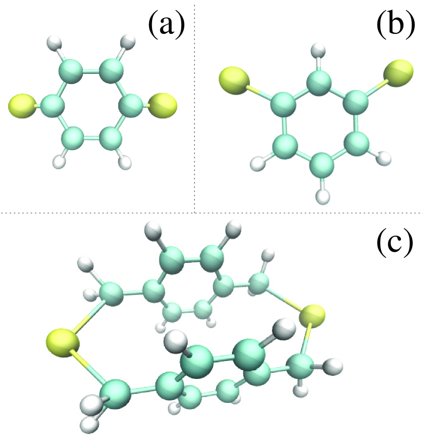
Figure 1: Molecular junctions used to illustrate the local-noise spectroscopy: (a) para-benzenedithiol (PBDT), (a) meta-benzenedithiol (MBDT), and (b) 2,11-dithi(3,3)paracyclophane molecular structures. The yellow circles represent the sulfur atoms that attach to two macroscopic electrodes.

III Numerical results

We are now ready to illustrate how the LNS, implemented in Eq. (10), may be used to analyze several physical properties in biased molecular junctions. We then consider three distinct molecular structures represented in Fig. 1: a benzenedithiol molecular junction in para (PBDT, Fig. 1a) and meta (MBDT, Fig. 1b) configuration, and a 2,11-dithia(3,3)paracyclophane molecular junction employed in measurements of quantum coherence in Ref. Vazquez et al. (2012) (Fig. 1c). Simulations of molecular electronic structure are performed within the Gaussian package Frisch et al. (2016) employing the Hartree-Fock level of the theory, and Slater-type orbitals with 3 primitive gaussians (STO-3g) basis set. The molecular structures are coupled to semi-infinite contacts via sulfur atoms; each orbital of the latter is assumed to support $\Gamma_{K}=0.1$ eV electron exchange rate between the molecule and contact $K$ ($L$ or $R$) Kinoshita et al. (1995). The contacts are modeled within the wide-band approximation Cabra et al. (2018). While this level of molecule-contacts modeling is enough for illustration purposes, actual ab initio simulations should use a better basis set and perform realistic self-energy calculations. The Fermi energy $E_{F}$ is taken to be $1$ eV above the highest occupied molecular orbital (HOMO) for the PBDT and MBDT junctions (Figs. 1a and b).

Following Ref. Vazquez et al. (2012) we take the Fermi energy in the middle of the highest occupied-lowest unoccupied molecular orbital (HOMO-LUMO) gap for the double-backbone molecular structure of Fig. 1c. Finally, the bias $V_{sd}$ across the junction is applied symmetrically: $\mu_{L,R}=E_{F}\pm|e|V_{sd}/2$. The numerical illustrations below are presented on plane(s) parallel to the molecular plane(s) at a distance of $1.5$ Å above it. Calculations are performed on a spatial grid spanning from $-4$ Å to $4$ Å with step of $0.25$ Å. The center of the coordinate system is chosen at the molecule’s center of mass.

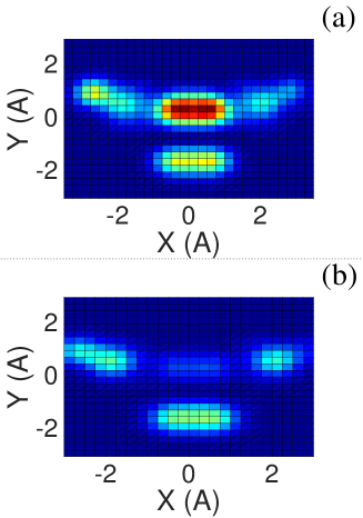
Figure 2: Electroluminiscence profile in a MBDT molecular junction (Fig. 1b) at $V_{sd}=3$ V. The profile is plotted parallel to the molecule at $1.5$ Å above the molecular plane. The horizontal axis ($X$) is the direction of tunneling in the junction. The localized surface plasmon-polariton vector is assumed to be directed along $X$. The light emission profiles are shown for the outgoing photons of frequencies (a) $\omega=2$ eV and (b) $3$ eV.

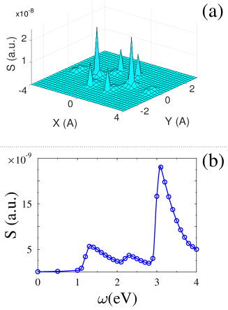
Figure 3: Local noise cross-correlation $S(\vec{r}_{1},\vec{r}_{2};\omega)=\sqrt{\sum_{i=\{x,y,z\}}S^{2}_{ii}(\vec{r}_{1},\vec{r}_{2};\omega)}$ in a 2,11-dithi(3,3)paracylophane molecular junction (Fig. 1c) at $V_{sd}=1$ V. The horizontal axis ($X$) is the direction of tunneling in the junction. The profile is plotted parallel to the molecular planes with $Z$ projections of $\vec{r}_{1}$ and $\vec{r}_{2}$ taken $1.5$ Å on outer sides of molecular planes. We show (a) the cross-correlation map in the $XY$ plane at $\omega=3.5$ eV, and (b) the cross-correlation at the points corresponding to positions of carbon atoms of the benzene rings vs. frequency $\omega$.

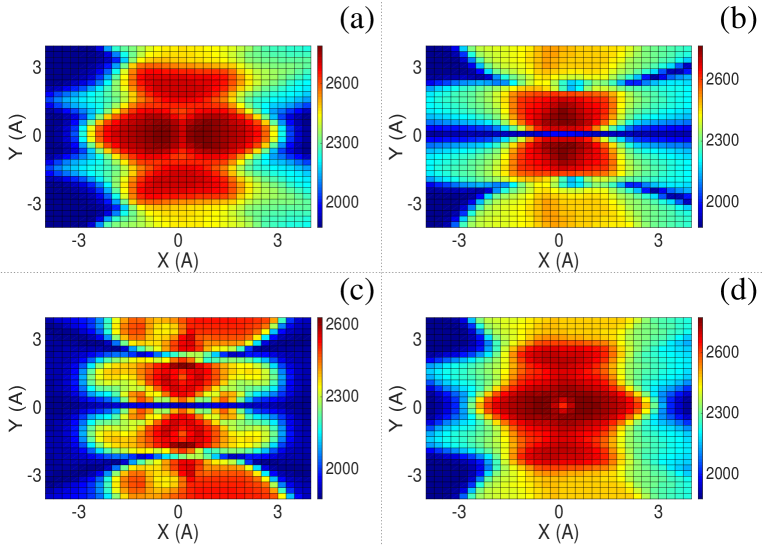
Figure 4: Local noise thermometry in a PBDT molecular junction (Fig. 1a) at a bias $V_{sd}=1$ V. The temperature distribution, Eq. (11), is plotted parallel to the molecule at $1.5$ Å above the molecular plane. The horizontal axis ($X$) is the direction of tunneling in the junction. The temperature estimates are shown from a non-invasive probe oriented (a) perpendicular to the junction tunneling direction, (b) parallel to the junction tunneling direction and perpendicular to the molecular plane, (c) parallel to the molecular plane, and (d) perpendicular to the local current. The vertical (color) bar shows the temperature scale in K.

Bias-induced light-emission – Let us first discuss bias-induced light emission in molecular junctions. The theory of light emission from quantum noise was recently put forward in Ref. Kaasbjerg and Nitzan (2015). It was shown that the emission is related to the positive frequency part of the asymmetric noise (the last row of Eq. (10)) in the plasmonic contact. The corresponding local noise distribution then yields the electroluminscence profile in a biased molecular junction. According to the theory of Ref. Kaasbjerg and Nitzan (2015), the local current projections are fixed by the direction of the localized surface plasmon-polariton vector.

Figure 2 shows the light emission in a MBDT molecular junction (Fig. 1b) at a bias $V_{sd}=3$ V. It is interesting to note that the outgoing photons of different frequencies probe different parts of the molecule (compare Figs. 2a and b). This fact cannot be extracted from other spectroscopic probes and is due to local features of the potential profile distribution in the junction.

Correlation effects in transport – As a second example, we discuss the local noise probed at two distinct points in space (cross-correlations) to detect inter-dependence of different paths in quantum transport. Using the latter as, e.g., indicator of inter-species spin interactions was discussed in Ref. Sinitsyn and Pershin (2016). To illustrate the usefulness of the concept in a non-equilibrium setting we consider a 2,11-dithi(3,3)paracylophane molecular junction (Fig. 1c). The junction provides two paths for electron tunneling, which lead to observation of constructive interference in transport Vazquez et al. (2012).

We probe the independence of the two paths by calculating the LNS cross-correlation map of local currents taken outside of the two molecules at a distance of $1.5$ Å away from the molecular planes. That is, $X$ and $Y$ projections ($XY$ is parallel to the molecular planes) of vectors $\vec{r}_{1}$ and $\vec{r}_{2}$ in (10) are taken equal to each other, while their $Z$ components are taken $1.5$ Å away on the outer side of molecular planes (see Fig. 1c). The resulting cross-correlation map is shown in Fig. 3. As expected, correlations between the two molecules show maxima at the positions of carbon atoms, where interaction between $p_{z}$ atomic orbitals of the atoms is significant (see Fig. 3a).

However, extra information can be extracted from the frequency dependence of the cross-correlation, which indicates a characteristic interaction energy scale in the system. Frequency dependence of cross-correlation corresponding to position of carbon atoms of the two benzene rings is shown in Fig. 3b. Three peaks indicate respectively the effective strengths of $2s-2s$, $2s-2p_{z}$, and $2p_{z}-2p_{z}$ atomic orbital couplings. The peaks approximately correspond to the Rabi frequency related to the Fock matrix couplings between orbitals of adjacent carbon atoms in the two molecules of the junction.

Local thermometry – We discuss here how to employ local-noise spectroscopy (LNS) as a local thermometry tool in current-carrying molecular junctions. Although a nonequilibrium state cannot be identified with a unique thermodynamic temperature, and experimentally measurable failures of attempts to introduce such characteristic were discussed in the literature Hartmann and Mahler (2005), the concept of temperature as a single parameter effectively describing bias-induced heating Huang et al. (2006) is attractive. For example, Raman measurements in current-carrying junctions were utilized to introduce an effective temperature of molecular vibrational and electronic degrees freedom Ioffe et al. (2008); Ward et al. (2011). Such assignment implies existence of some sort of local equilibrium. As a measure of electronic temperature an idea of equilibrium probe with chemical potential and temperature adjusted in such a way that no particle and energy fluxes exist between the probe and nonequilibrium electronic distribution was put forward and utilized in a number of studies Dubi and Di Ventra (2011); Galperin and Nitzan (2011a, b).

In the context of noise spectroscopy, it was indeed recently suggested that noise may be used to measure electronic temperatures Tikhonov et al. (2016); Weng et al. (2018). Here, we follow the suggestion of Ref. Weng et al. (2018), and utilize the equilibrium noise expression Blanter and Buttiker (2000); Di Ventra (2008), $S=4k_{B}TG$ (with $G$ the conductance), and the fact that at zero bias the molecular temperature should correspond to that of the contacts, to introduce a nonequilibrium effective local temperature $T_{M}(A)$ as a function of the noise in Eq. (9)

$$T_{M}(A)=T_{0}\,\frac{S_{AA}(\omega=0)\lvert_{V_{sd}}}{S_{AA}(\omega=0)\lvert_{0}}.$$ (11)

Here, $T_{0}$ is the temperature in the contacts (assumed to be $300$ K in both $L$ and $R$ reservoirs), $A$ is the surface area of a non-invasive probe that measures the local temperature Dubi and Di Ventra (2011).

Note that for small surface areas ($A=6.25\times 10^{-2}$ Å²), over which the integrands in Eq. (9) are constants, the area size $A$ dependence disappears. This is the case discussed here. As a test case we consider the PBDT molecular junction shown in Fig. 1a.

Figure 4 shows the temperature distribution in the PBDT molecular junction calculated using Eq. (11) at $V_{sd}=1$ V. We assume a non-invasive probe, which measures local noise of the current projections perpendicular to the probe’s surface at a distance of $1.5$ Å above the molecular plane. Fig. 4 shows that while the temperature values are of the same order of magnitude, the temperature profiles are substantially different for different probe orientations. Of course, in realistic measurements the probe is always invasive and the experimentally measured profiles will mix different contributions. However, such dependence on orientation may be observable under certain conditions. For example, the effect may be observable in measurements in graphene nano-ribbons. This also confirms that the definition of temperature is not unique in a non-equilibrium setting and depends on the type of probes used to define it Dubi and Di Ventra (2011); Galperin and Nitzan (2011b).

IV Conclusion

We have introduced the concept, and developed the theory of local-noise spectroscopy as a tool to study transport properties of systems out of equilibrium. The concept is a natural extension of local fluxes which have been used to characterize charge (and energy) flow in nanoscale systems.

We have shown that the local noise contains rich and complementary (to local fluxes) information on the system. In particular, we have exemplified this tool with the study of bias-induced light emission, intra-system interactions in molecular junctions, and discussed its application to nano-thermometry.

In the case of light emission we find that outgoing photons of different frequencies may probe different regions of the molecule, an interesting effect difficult to extract from other probes. The cross-correlations of the local noise are instead an indicator of intra-system interactions, and its frequency dependence yields information on their interaction strength and relevant energy scale. Finally, in the case of nano-thermometry we predict temperature profiles dependent on the different probe orientations.

Although LNS may, at the moment, be difficult to realize experimentally, our work shows that it can already be of great help as a theoretical tool to analyze a wide variety of physical properties in different non-equilibrium systems. We thus hope that our work will motivate experimentalists in pursuing this line of research that may lead to another important spectroscopic probe with the potential to unravel phenomena difficult to detect with other techniques.