Optimizing Organizations for Navigating Data Lakes

Abstract

We consider the problem of creating a navigation structure that allows a user to most effectively navigate a data lake. We define an organization as a graph that contains nodes representing sets of attributes within a data lake and edges indicating subset relationships among nodes. We present a new probabilistic model of how users interact with an organization and define the likelihood of a user finding a table using the organization. We propose the data lake organization problem as the problem of finding an organization that maximizes the expected probability of discovering tables by navigating an organization. We propose an approximate algorithm for the data lake organization problem. We show the effectiveness of the algorithm on both real data lakes containing data from open data portals and on benchmarks that emulate the observed characteristics of real data lakes. Through a formal user study, we show that navigation can help users discover relevant tables that cannot be found by keyword search. In addition, in our study, 42% of users preferred the use of navigation and 58% preferred keyword search, suggesting these are complementary and both useful modalities for data discovery in data lakes. Our experiments show that data lake organizations take into account the data lake distribution and outperform an existing hand-curated taxonomy and a common baseline organization.

1 Introduction

The popularity and growth of data lakes is fueling interest in dataset discovery. Dataset discovery is normally formulated as a search problem. In one version of the problem, the query is a set of keywords and the goal is to find tables relevant to the keywords DBLP:conf/www/BrickleyBN19 ; Pimplikar:2012 . Alternatively, the query can be a table (a query table), and the problem is to find other tables that are close to the query table Cafarella:2009 . If the input is a query table, then the output may be tables that join or union with query table NargesianZPM18 ; DasSarma:2012 ; Zhu:2016 ; ZhuDNM19 ; YangZYZLY18 .

A complementary alternative to search is navigation. In this paradigm, a user navigates through an organizational structure to find tables of interest. In the early days of Web search, navigation was the dominant discovery method for Web pages. Yahoo!, a mostly hand-curated directory structure, was the most significant internet gateway for Web page discovery Yahoo . Even today, hierarchical organizations of Web content (especially entities like videos or products) is still used by companies such as Youtube.com and Amazon.com. Hierarchical navigation allows a user to browse available entities going from more general concepts to more specific concepts using existing ontologies or structures automatically created using taxonomy induction Snow:2006:STI ; Kozareva:2010 ; Yang:2009 . When entities have known features, we can apply faceted-search over entities zheng2013survey ; KorenZL08 ; velardi2013ontolearn . Taxonomy induction looks for is-a relationships between entities (e.g., student is-a person), faceted-search applies predicates (e.g., model = volvo) to filter entity collections Arenas:2016:FSO . In contrast to hierarchies over entities, in data lakes tables contain attributes that may mention many different types of entities and relationships between them. There may be is-a relationships between tables, or their attributes, and no easily defined facets for grouping tables. If tables are annotated with class labels of a knowledge base (perhaps using entity-mentions in attribute values), the is-a relationships between class labels could provide an organization on tables. However, recent studies show the difference in size and coverage of domains in various public cross-domain knowledge bases and highlight that no single public knowledge base sufficiently covers all domains and attribute values represented in heterogeneous corpuses such as data lakes hassanzadeh2015understanding ; Ritze:2016:PPW:2872427.2883017 . In addition, the coverage of standard knowledge bases on attribute values in open data lakes is extremely low NargesianZPM18 . Knowledge bases are also not designed to provide effective navigation. We propose instead to build an organization that is designed to best support navigation and exploration over heterogeneous data lakes. Our goal is not to compete with or replace search, but rather to provide an alternative discovery option for users with only a vague notion of what data exists in a lake.

1.1 Organizations

Dataset or table search is often done using attributes by finding similar, joinable, or unionable attributes DasSarma:2012 ; fernandez2018aurum ; fernandez2018seeping ; NargesianZPM18 ; Zhu:2016 ; ZhuDNM19 . We follow a similar approach and define an organization as a Directed Acyclic Graph (DAG) with nodes that represent sets of attributes from a data lake. A node may have a label created from the attribute values themselves or from metadata when available. A table can be associated to all nodes containing one or more of its attributes. An edge in this DAG indicates that the attributes in a parent node is a superset of the attributes in a child node. A user finds a table by traversing a path from a root of an organization to any leaf node that contains any of its attributes.

We propose the data lake organization problem where the goal is to find an organization that allows a user to most efficiently find tables. We describe user navigation of an organization using a Markov model. In this model, each node in an organization is equivalent to a state in the navigation model. At each state, a user is provided with a set of next states (the children of the current state). An edge in an organization indicates the transition from the current state to a next state. Due to the subset property of edges, each transition filters out some attributes until the navigation reaches attributes of interest. An organization is effective if certain properties hold. At each step, a user should be presented with only a reasonable number of choices. We call the maximum number of choices the branching factor. The choices should be distinct (as dissimilar as possible) to make it easier for a user to choose the most relevant one. The transition probability function of our model assumes users choose the next state that has the highest similarity to the topic query they have in mind. Also, the number of choices they need to make (the length of the discovery path) should not be large. Furthermore, in real data lakes, as we have observed and report in detail in our evaluation (Section 5), the topic distribution is typically skewed (with a few tables on some topics and a large number on others). Hence, give the typical skew of topics in real data lakes, a data lake organization must be able to automatically determine over which portions of the data, more organizational structure is required, and where a shallow structure is sufficient.

Table 1: Some Tables from Open Data.

Id	Table Name
d1	Surveys Data for Olympia Oysters, Ostrea lurida, in BC
d2	Sustainability Survey for Fisheries
d3	Grain deliveries at prairie points 2015-16
d4	Circa 1995 Landcover of the Prairies
d5	Mandatory Food Inspection List
d6	Canadian Food Inspection Agency (CFIA) Fish List
d7	Wholesale trade, sales by trade group
d8	Historical releases of merchandise imports and exports
d9	Immigrant income by period of immigration, Canada
d10	Historical statistics, population and immigrant arrivals

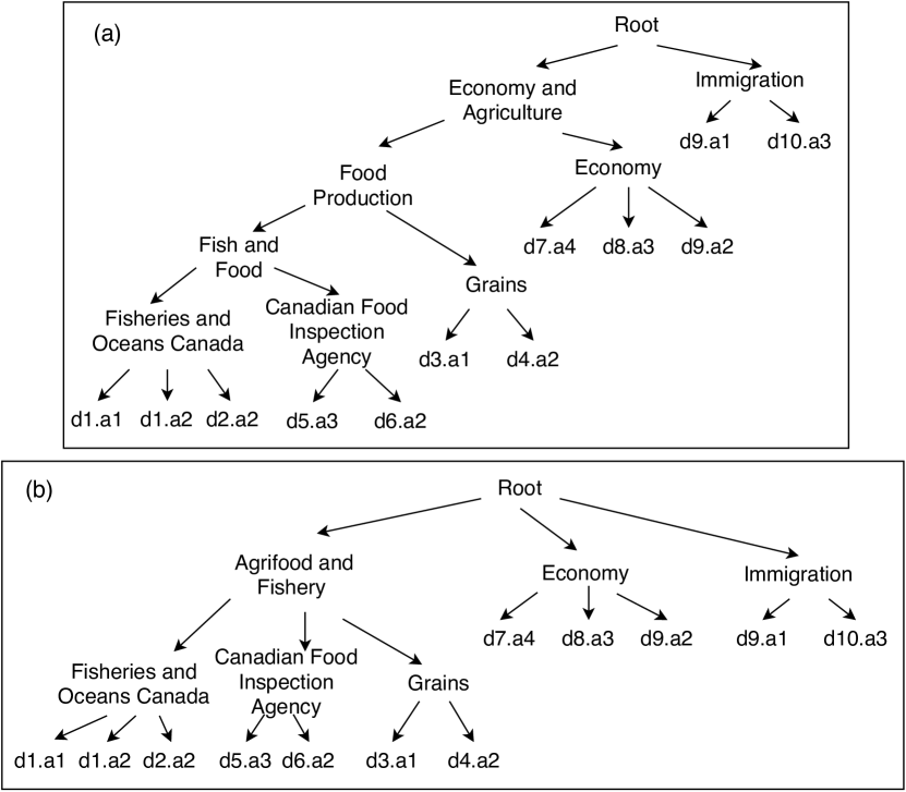
Figure 1: (a) Deep and (b) Effective Organization.

Example 1.

Consider the (albeit small) collection of tables from a data lake of open data tables (Table 1). A table can be multi-faceted and attributes in a table can be about different topics. One way to expose this data to a user is through a flat structure of attributes of these tables. A user can browse the data (and any associated metadata) and select data of interest. If the number of tables and attributes is large, it would be more efficient to provide an organization over attributes. Suppose the tables are organized in the DAG of Figure 1(a). The label of a non-leaf node in this organization summarizes the content of the attributes in the subgraph of the node. Suppose a user is interested in the topic of food inspection. Using this organization, at each step of navigation, they have to choose between only two nodes. The first two choices seem clear, Economy and Agriculture and Food Production seem more relevant to the user than their alternatives (Immigration and Economy). However, having a small branching factor in this organization results in nodes that may be misleading. For example, it may not be clear if there is any inspection data under the node Fish and Food or under Grains. This is due to the large heterogeneity of attributes (like Oysters and Grain Elevators) in the organization below the Fish and Food node. The organization in Figure 1(b) addresses this problem by organizing attributes of Grains, Food Inspection, and Fisheries at the same level. Note that this organization has a higher branching factor, but the choices are more distinct at each node.

1.2 Contributions

We define an organization as a DAG on nodes consisting of subsets of attributes in a data lake. We propose a navigation model on an organization which models the user experience during discovery. We define when an organization is optimal in that it is best suited to help a user find any attribute of interest in a small number of navigation steps without having to consider an excessive number of choices or choices that are indistinct.

We make the following contributions.

• We propose to model navigation as a Markov model, which computes the probability of discovering a table that is relevant to a topic of interest. We define the data lake organization problem as the problem of finding an organization that maximizes the expected probability of discovering lake tables, namely the effectiveness of the organization.

• We propose a local search algorithm that approximates an optimal organization. Particularly, we consider the organization problem as a structure optimization problem in which we explore subsets of the power-set lattice of organizations.

• To reduce the complexity of search, the local search algorithm leverages the lake metadata when it is available. We propose an approximate and efficient way of comparing organizations during search and provide an upper bound for the error of this approximation.

• We propose a metadata enrichment algorithm that effectively bootstraps any existing metadata. Our experiments show that metadata can be transferred across data lakes.

• Our experiments show that organizations are able to optimize navigation based on lake data distribution and outperform a hand-curated taxonomy. We show that the organization constructed by our algorithm outperforms a baseline and an existing linkage graph on a real data lake containing open government data.

• Through a user-study comparing navigation to keyword search, we show that while there is no statistical difference in the number of relevant tables found, navigation can help users find a more diverse set of tables than keyword search. In addition, in our study, 42% preferred the use of navigation over keyword search (the others preferred search), suggesting these are complementary and both useful modalities for dataset discovery in data lakes.

2 Foundations

We describe a probabilistic model of how users navigate a data lake. We envision scenarios in which users interactively navigate through topics in order to locate relevant tables. The topics are derived and organized based on attributes of tables. Our model captures user elements such as the cognitive effort associated with multiple choices and the increasing complexity of prolonged navigational steps. We then define the data lake organization problem as the optimization problem of finding the most effective organization for a data lake.

2.1 Organization

Let $\mathcal{T}$ be the set of all tables in a data lake. Each table $T\in\mathcal{T}$ consists of a set of attributes, $\mathrm{attr}(T)$. Let $\mathcal{A}$ be the set of all attributes, $\mathcal{A}=\bigcup\{\mathrm{attr}(T):T\in\mathcal{T}\}$ in a data lake. Each attribute $A$ has a set of values that we call a domain and denote by $\mathrm{dom}(A)$. An organization $\mathcal{O}=(V,E)$ is a DAG. Let $\operatorname{ch}(.)$ be the child relation mapping a node to its children, and $\operatorname{par}(.)$ be the parent relation mapping a node to its parents. A node $s\in V$ is a leaf if $\operatorname{ch}(s)=\emptyset$, otherwise $s$ is an interior node in $\mathcal{O}$. Every leaf node $s$ of $\mathcal{O}$ corresponds to a distinct attribute $A_{s}\in\mathcal{A}$. Each interior node $s$ corresponds to a set of attributes $D_{s}\subseteq\mathcal{A}$. If $c\in ch(s)$, then $D_{c}\subseteq D_{s}$, we call this the inclusion property, and $D_{s}=\bigcup_{c\in ch(s)}D_{c}$. We denote the domain of a state $s$ by $\mathrm{dom}(s)$ which is $\mathrm{dom}(A_{s})$ when $s$ is a leaf node and $\bigcup_{A\in D_{s}}\mathrm{dom}(A)$ otherwise.

2.2 Navigation Model

We model a user’s experience during discovery using an organization $\mathcal{O}$ as a Markov model where states are nodes and transitions are edges. We will use the terms state and node interchangably. Because of the inclusion property, transitions from a state filter out some of the attributes of the state. Users select a transition at each step and discovery stops once they reach a leaf node. To define the effectiveness of an organization, we define a user’s intent using a query topic $X$ modeled as a set of values. Starting at the root node, a user navigates through sets of attributes (states) ideally finding attributes of interest. In our definition of effectiveness, we assume the probability of a user’s transition from $s$ to $c\in\operatorname{ch}(s)$ is determined by the similarity between $X$ and the values of the attributes in $D_{c}$.

Example 2.

Returning to Example 1, to evaluate (and compare) the effectiveness of the two organizations in Figure 1 for a specific user topic like $X=$ ”food inspection” we can compute the similarity of this topic to the values in the attributes of the various nodes in each organization.

Note that when an organization is being used, we do not know $X$. Rather we are assuming that a user performs navigation in a way that they choose nodes that are closest to their (unknown to us) intended topic query. The concept of a user’s query topic is used only to build a good organization. We define an optimization problem where we build an organization that maximizes the expected probability of finding any table in the data lake by finding any of its attributes (assuming a user could potentially have in mind any attribute in the lake). In other words, the set of query topics we optimize for is the set of attributes in the lake.

2.3 Transition Model

We define the transition probability of $P(\mbox{$c$}|s,X,\mathcal{O})$ as the probability that the user will choose the next state as $c$ if they are at the state $s$. The probability should be correlated to the similarity between $\mathrm{dom}(\mbox{$c$})$ and $X$. Let $\kappa(c,X)$ be a similarity metric between $\mathrm{dom}(\mbox{$c$})$ and $X$. The transition probability is as follows.

$$P(\mbox{$c$}|s,X,\mathcal{O})=\frac{e^{\frac{\gamma}{|\operatorname{ch}(s)|}.\kappa(c,X)}}{\sum_{t\in ch(s)}e^{\frac{\gamma}{|\operatorname{ch}(s)|}.\kappa(t,X)}}$$ (1)

The constant $\gamma$ is a hyper parameter of our model. It must be a strictly positive number. The term $|\operatorname{ch}(s)|$ is a penalty factor to avoid having nodes with too many children. The impact of the high similarity of a state to $X$ diminishes when a state has a large branching factor.

A discovery sequence is a path, $r=s_{1},\ldots,s_{k}$ where $s_{i}\in ch(s_{i-1})$ for $1<i\leq k$. A state in $\mathcal{O}$ is reached through a discovery sequence. The Markov property says that the probability of transitioning to a state is only dependent on its parent. Thus, the probability of reaching state $s_{k}$ through a discovery sequence $r=s_{1},\ldots,s_{k}$, while searching for $X$ is defined as follows.

$$P(s_{k}|r,X,\mathcal{O})=\prod_{i=1}^{k}P(s_{i}|s_{i-1},X,\mathcal{O})$$ (2)

In this model, a user makes transition choices only based on the current state and the similarity of their query topic $X$ to each of the child states. Note that the model naturally penalizes long sequences. Since an organization is a DAG, a state can be reached by multiple discovery sequences. The probability of reaching a state $s$ in $\mathcal{O}$ while searching for $X$ is as follows.

$$P(s|X,\mathcal{O})=\sum_{r\in Paths(s)}P(s|r,X,\mathcal{O})$$ (3)

where $Paths(s)$ is the set of all discovery sequences in $\mathcal{O}$ that reach $s$ from the root. Additionally, the probability of reaching a state can be evaluated incrementally.

$$P(s|X,\mathcal{O})=\sum_{p\in par(s)}P(s|p,X,\mathcal{O})P(p|X,\mathcal{O})$$ (4)

Definition 1.

The discovery probability of an attribute $A$ in organization $\mathcal{O}$ is defined as $P(s|A,\mathcal{O})$, where $s$ is a leaf node. We denote the discovery probability of $A$ as $P(A|\mathcal{O})$.

2.4 Organization Discovery Problem

A table $T$ is discovered in an organization $\mathcal{O}$ by discovering any of its attributes.

Definition 2.

For a single table $T$, we define the discovery probability of a table as

$$P(T|\mathcal{O})=1-\prod_{A\in T}(1-P(A|\mathcal{O}))$$ (5)

For a set of tables $\mathcal{T}$ the organization effectiveness is

$$P(\mathcal{T}|\mathcal{O})=\frac{1}{|\mathcal{T}|}\sum_{T\in\mathcal{T}}P(T|\mathcal{O})$$ (6)

For a data lake, we define the data lake organization problem as finding an organization that has the highest organization effectiveness over all tables in the lake.

Definition 3.

Data Lake Organization Problem. Given a set of tables $\mathcal{T}$ in a data lake, the organization problem is to find an organization $\hat{\mathcal{O}}$ such that:

$$\hat{\mathcal{O}}=\operatorname*{arg\,max}_{\mathcal{O}}P(\mathcal{T}|\mathcal{O})$$ (7)

We remark that in this model we do not assume the availability of any query workloads. Since our model uses a standard Markov model, we can apply existing incremental model estimation techniques DBLP:journals/isci/KhreichGMS12 to maintain and update the transition probabilities as behavior logs and workload patterns become available through the use of an organization by users.

2.5 Multi-dimensional Organizations

Given the heterogeneity and massive size of data lakes, it may be advantagous to perform an initial grouping or clustering of tables and then build an organization on each cluster.

Example 3.

Consider again the tables from Example 1 which come from real government open data. To build an organization over a large open data lake, we can first cluster tables (e.g., using ACSDb which clusters tables based on their schemas DBLP:journals/pvldb/CafarellaHWWZ08 or using a clustering over the attribute values or other features of a table) DBLP:journals/pvldb/CafarellaHK09 . This would define (possibly overlapping) groups of tables, perhaps a group on Immigration data and another on Environmental data over which we may be able to build more effective organizations.

If we have a grouping of $\mathcal{A}$ into $k$ (possibly overlapping) groups or dimensions, $G_{1},\ldots,G_{k}$, then we can discover an organization over each and use them collectively for navigation. We define a $k$-dimensional organization $\mathcal{M}$ for a data lake $\mathcal{T}$ as a set of organizations $\{\mathcal{O}_{1},\ldots,\mathcal{O}_{k}\}$, such that attributes of each table in $\mathcal{T}$ is organized in at least one organization and $\mathcal{O}_{i}$ is the most effective organization for $G_{i}$. We define the probability of discovering table $T$ in $\mathcal{M}$, as the probability of discovering $T$ in any of dimensions of $\mathcal{M}$.

$$P(T|\mathcal{M})=1-\prod_{\mathcal{O}_{i}\in\mathcal{M}}(1-P(T|\mathcal{O}_{i}))$$ (8)

3 Constructing Organizations

Given the abstract model of the previous section, we now present a specific instantiation of the model that is suited for real data lakes. We justify our design choices using lessons learned from search-based table discovery. We then consider the metadata that is often available in data lakes, specifically table-level tags, and explain how this metadata (if available) can be exploited for navigation. Finally, we present a local search algorithm for building an approximate solution for the data lake organization problem.

3.1 Attribute and State Representation

We have chosen to construct organizations over the text attributes of data lakes. This is based on the observation that although a small percentage of attributes in a lake are text attributes (26% for a Socrata open data lake that we use in our experiments), the majority of tables (92%) have at least one text attribute. We have found that similarity between numerical attributes (measured by set overlap or Jaccard) can be very misleading as attributes that are semantically unrelated can be very similar and semantically related attributes can be very dissimilar. Hence, to use numerical attributes one would first need to understand their semantics. Work is emerging on how to do this DBLP:conf/cikm/IbrahimRW16 ; DBLP:conf/kdd/HulsebosHBZSKDH19 ; DBLP:conf/icde/IbrahimRWZ19 .

Since an organization is used for the exploration of heterogeneous lakes, we are interested in the semantic similarity of values. To capture semantics, a domain can be canonicalized by a set of relevant class labels from a knowledge base Limaye:2010:ASW ; venetis2011recovering ; DBLP:conf/kdd/HulsebosHBZSKDH19 . We have found that open knowledge bases have relatively low coverage on data lakes NargesianZPM18 . Hence, we follow an approach which has proven to be successful in search-based table discovery which is to represent attributes by their collective word embedding vectors NargesianZPM18 .

Each data value $v$ is represented by an embedding vector $\vec{v}$ such that values that are more likely to share the same context have embedding vectors that are close in embedding space according to an Euclidean or angular distance measure Mikolov:2013 . Attribute $A$ can be represented by a topic vector, $\mu_{A}$, which is the sample mean of the population $\{\vec{v}|v\in\mathrm{dom}(A)\}$ NargesianZPM18 . In organization construction, we also represent $X$ by $\mu_{X}$.

Definition 4.

State $s$ is represented with a topic vector, $\mu_{s}$, which is the sample mean of the population $\{\vec{v}|v\in\mathrm{dom}(s)\}$.

If a sufficient number of values have word embedding representatives, the topic vectors of attributes are good indicators of attributes’ topics. We use the word embeddings of fastText database joulin:2016 , which on average covers 70% of the values in the text attributes in the datasets used in our experiments. In organization construction, to evaluate the transition probability of navigating to state $c$ we choose $\kappa(\mbox{$c$},X)$ to be the Cosine similarity between $\mu_{\mbox{$c$}}$ and $\mu_{X}$. Since a parent subsumes the attributes in its children, the Cosine similarity satisfies a monotonicity property of $\kappa(X,\mbox{$c$})>\kappa(X,s)$, where $\mbox{$c$}\in ch(s)$. However, the monotonicity property does not necessarily hold for the transition probabilities. This is because $P(\mbox{$c$}|s,X,O)$ is normalized with all children of parent $s$.

3.2 State Space Construction

Metadata in Data Lakes

Tables in lakes are sometimes accompanied by metadata hand-curated by the publishers and creators of data. In enterprise lakes, metadata may come from design documentation from which tags or topics can be extracted. For open data, the standard APIs used to publish data include tags or keywords DBLP:journals/debu/MillerNZCPA18 . In mass-collaboration datasets, like web tables, contextual information can be used to extract metadata hassanzadeh2015understanding .

State Construction

If metadata is available, it can be distilled into tags (e.g., keywords, concepts, or entities). We associate these table-level tags with every attribute in the table. In an organization, the leaves still have a single attribute, but the immediate parent of a leaf is a state containing all attributes with a given (single) tag. We call these parents tag states. Building organizations on tags reduces the number of possible states and the size of the organization while still having meaningful nodes that represent a set of attributes with a common tag.

Example 4.

In the organization of Figure 1 (b) we have actually used real tags from open data to label the internal nodes (with the exception of Agrifood and Fishery which is our space saving representation of a node representing the three real tags: Canadian Food Inspection Agency, Fisheries and Oceans Canada and Grains). Instead of building an organization over the twelve attributes, we can build a smaller organization over the five tags: Canadian Food Inspection Agency, Fisheries and Oceans Canada, Grains, Economy, and Immigration.

Definition 5.

Let $\mathrm{data}(t)$ be the relation mapping a tag $t$ in a lake metadata to the set of its associated attributes. Suppose $M_{s}$ is the set of tags in a tag state $s$. Thus, the set of attributes in $s$ is $D_{s}=\bigcup_{t\in M_{s}}\mathrm{data}(t)$. A tag state $s$ is represented with a topic vector, $\mu_{s}$, which is the sample mean of the population $\{\vec{v}|v\in\mathrm{dom}(A),A\in D_{s}\}$.

Flat Organization: A Baseline

In the organization, we consider the leaves to be states with one attribute. However, now the parent of a leaf node is associated to only one tag. This means that the last two levels of a hierarchy are fixed and an organization is constructed over states with a single tag. If instead of discovery, we place a single root node over such states, we get a flat organization that we can use as a baseline. This is a reasonable baseline as it is conceptually, the navigation structure supported by many open data APIs that permit programmatic access to open data resources. These APIs permit retrieval of tables by tag.

Enriching Metadata

Building organizations on tags reduces organization discovery cost. However, the tags coming from the metadata may be incomplete (some attributes may have no tags). Moreover, the schema and vocabulary of metadata across data originating from different sources may be inconsistent which can lead to disconnected organizations. We propose to transfer tags across data lakes such that data lakes with no (or little) metadata are augmented with the tags from other data lakes. To achieve this, we build binary classifiers, one per tag, which predict the association of attributes to the corresponding tags. The classifiers are trained on the topic vector, $\mu_{A}$, of attributes. Attributes that are associated to a tag are the positive training samples for the tag’s classifier and the remaining attributes are the negative samples. This results in imbalanced training data for large lakes. To overcome this problem, we only use a subset of negative samples for training. We consider the ratio of positive and negative samples as a hyperparameter.

3.3 Local Search Algorithm

Algorithm 1 Algorithm Organize

1:procedure Organize($\mathcal{T}$)

2:     $mod\_ops=[\textsc{Delete\_Parent},\textsc{Add\_Parent}]$

3:     $\mathcal{O}\leftarrow\textsc{Init\_Org}(\mathcal{T})$, $p\leftarrow\textsc{eval}(\mathcal{O})$

4:     while $\neg termination\_cond$ do

5:         $state\leftarrow\textsc{state\_to\_modify}(\mathcal{O})$

6:         $\mathcal{O}^{\prime}\leftarrow\textsc{choose\_apply\_op}(\mathcal{O},state,mod\_ops)$

7:         if $\textsc{accept}(\textsc{eval}(\mathcal{O}^{\prime}),p)$ then

8:              $\mathcal{O}\leftarrow\mathcal{O}^{\prime},p\leftarrow p^{\prime}$

9:         end if

10:     end while

11:     return $\mathcal{O}$

12:end procedure

Our local seach algorithm, Organize, is outlined in Algorithm 1. It begins with an initial organization (Line 3). At each step, the algorithm proposes a modification to the current organization $\mathcal{O}$ which leads to a new organization $\mathcal{O}^{\prime}$ (Line 6). If the new organization is closer to a solution for the Data Lake Organization Problem (Definition 3), it is accepted as the new organization, otherwise it is accepted (Line 7) with a propability that is a ratio of the effectiveness, namely FriedmanK03 :

$$min[1,\frac{P(\mathcal{T}|\mathcal{O}^{\prime})}{P(\mathcal{T}|\mathcal{O})}]$$ (9)

The algorithm terminates (Line 4) once the effectiveness of an organization reaches a plateau. In our experiments, we terminate when the expected probability has not improved significantly for the last 50 iterations.

We heuristically try to maximize the effectiveness of an organization by making its states highly reachable. We use Equation 4 to evaluate the probability of reaching a state when searching for attribute $A$ and define the overall reachability probability of a state as follows.

$$P(s|\mathcal{O})=\frac{1}{|A\in\mathcal{T}|}\sum_{A\in\mathcal{T}}P(s|A,\mathcal{O})$$ (10)

Starting from an initial organization, the search algorithm performs downward traversals from the root and proposes a modification on the organization for states in each level of the organization ordered from lowest reachability probability to highest (Line 5 and 6). A state is in level $l$ if the length of the shortest discovery paths from root to the state is $l$. We restrict our choices of a new organization at each search step to those created by two operations.

Operation I: Adding Parent

Given a state $s$ with low reachability probability, one reason for this may be that it is one child amongst many of its current parent, or that it is indistinguishable from a sibling. We can remedy either of these by adding a new parent for $s$. Suppose that the search algorithm chooses to modify the organization with respect to state $s$. Recall that Equation 4 indicates that the probability of reaching a state increases as it is connected to more parent states. Suppose $s$ is at level $l$ of organization $\mathcal{O}$. The algorithm finds the state, called $n$, at level $l-1$ of $\mathcal{O}$ such that it is not a parent of $s$ and has the highest reachability probability among the states at $l-1$. To satisfy the inclusion property, we update node $n$ and its ancestors to contain the attributes in $s$, $D_{s}$. To avoid generating cycles in the organization, the algorithm makes sure that none of the children of $s$ is chosen as a new parent. State $n$ is added to the organization as a new parent of $s$. Figure 2a shows an example of ADD_PARENT operation. ADD_PARENT potentially increases the reachability probability of a state by adding more discovery paths ending at that state, at the cost of increasing the branching factor.

Example 5.

For example, the attribute d6.a2 from table Canadian Food Inspection Agency (CFIA) Fish List in the organization of Figure 1(b) is reachable from the node with the tag Canadian Food Inspection Agency. This attribute is also related to the node with the tag Fisheries and Oceans Canada and can be discovered from that node. The algorithm can decide to add an edge from Fisheries and Oceans Canada to d6.a2 and make this state its second parent.

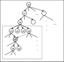
(a)

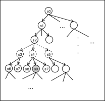
(b)

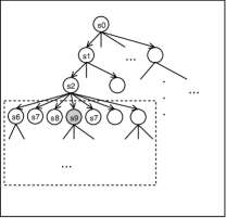
(c)

Figure 2: (a) Before and After Applying Add_Parent Operation, (b) Before and (c) After Applying Delete_Parent Operation.

Operation II: Deleting Parent

Another reason a state can have low reachability is that its parent has low reachability probability and we should perhaps remove a parent. Reducing the length of paths from the root to state $s$ is a second way to boost the reachability probability of $s$. The operation eliminates the least reachable parent of $s$, called $r$. To reduce the height of $\mathcal{O}$, the operation eliminates all siblings of $r$ except the ones with one tag. Then, it connects the children of each eliminated state to its parents. Figures 2b and 2c show an example of applying this operation on an organization. This makes the length of paths to $s$ smaller which boosts the reachability probability of $s$. However, replacing the children of a state by all its grandchildren increases the branching factor of the state, thus, decreasing the transition probabilities from that state.

Example 6.

For example, the algorithm can decide to eliminate the state Economy and Agriculture in the organization of Figure 1(a) and connect its children directly to the root.

In Algorithm 1, STATE_TO_MODIFY (Line 5) orders states by level starting at level 1 and within a level by reachability (lowest to highest) and returns the next state each time it is called. CHOOSE_APPLY_OP picks the operator that when applied creates the most effective organization $\mathcal{O}^{\prime}$. Everytime a new organization is chosen, STATE_TO_MODIFY may need to reorder states appropriately.

Initial organization

(Line 3) The initial organization may be any organization that satisfies the inclusion property of attributes of states. For example, the initial organization can be the DAG defined based on a hierarchical clustering of the tags of a data lake.

4 Scaling Organization Search

The search algorithm makes local changes to an existing organization by applying operations. An operation is successful if it increases the effectiveness of an organization. The evaluation of the effectiveness (Equation 7) involves computing the discovery probability for all attributes which requires evaluating the probability of reaching the states along the paths to an attribute (Equation 4). The organization graph can have a large number of states, especially at the initialization phase. To improve the search efficiency, we first identify the subset of states and attributes whose discovery probabilities may be changed by an operation and second we approximate the new discovery probabilities using a set of attribute representatives.

4.1 States Affected by an Operation

At each search iteration we only re-evaluate the discovery probability of the states and attributes which are affected by the local change. Upon applying Delete_Parent on a state, the transition probabilities from its grandparent to its grandchildren are changed and consequently all states reachable from the grandparent. However, the discovery probability of states that are not reachable from the grandparent remain intact. Therefore, for Delete_Parent, we only re-evaluate the discovery probability of the states in the sub-graph rooted by the grandparent and only for attributes associated to the leaves of the sub-graph.

The Add_Parent operation impacts the organization more broadly. Adding a new parent to a state $s$ changes the discovery probability of $s$ and all states that are reachable from $s$. Furthermore, the parent state and consequently its ancestors are updated to satisfy the inclusion property of states. Suppose the parent itself has only one parent. The change of states propagates to all states up to the lowest common ancestor (LCA) of $s$ and its parent-to-be before adding the transition to the organization. If the parent-to-be has multiple parents the change needs to be propagated to other subgraphs. To identify the part of the organization that requires re-evaluation, we iteratively compute the LCA of $s$ and each of the parents of its parent-to-be. All states in the sub-graph of the LCA require re-evaluation.

4.2 Approximating Discovery Probability

Focusing on states that are affected by operations reduces the complexity of the exact evaluation of an organization. To further speed up search, we evaluate an organization on a small number of attribute representatives. that each summarizes a set of attributes. The discovery probability of each representative approximates the discovery probability of its corresponding attributes. We assume a one-to-one mapping between representatives and a partitioning of attributes. Suppose $\rho$ is a representative for a set of attributes $D_{\rho}=\{A_{1},\ldots,A_{m}\}$. We approximate $P(A_{i}|\mathcal{O})$, $A_{i}\in D_{\rho}$ with $P(\rho|\mathcal{O})$. The choice and the number of representatives impact the error of this approximation.

Now, we describe an upper bound for the error of the approximation. Recall that the discovery probability of a leaf state is the product of transition probabilities along the path from root to the state. To determine the error that a representative introduces to the discovery probability of an attribute, we first define an upper bound on the error incurred by using representatives in transition probabilities. We show that the error of transition probability from $m$ to $s$ is bounded by a fraction of the actual transition probability which is correlated with the similarity of the representative to the attribute. Recall the transition probability from Equation 1. For brevity, we assume $\gamma^{\prime}=\frac{\gamma}{|ch(m)|}$.

$$P(s_{i}|m,A,\mathcal{O})=\frac{e^{\gamma^{\prime}\kappa(A,s_{i})}}{\sum_{s_{j}\in ch(m)}e^{\gamma^{\prime}\kappa(A,s_{j})}}$$ (11)

Suppose $\delta$ is the distance metric of the metric $\kappa$, which is $\delta(a,b)=1-\kappa(a,b)$. From the triangle property, it follows that:

$$\delta(s_{i},\rho_{k})\leq\delta(s_{i},A)+\delta(A,\rho)$$ (12)

Evaluating $P(s_{i}|m,A,\mathcal{O})$ and $P(s_{i}|m,\rho,\mathcal{O})$ requires computing $\kappa(A,s_{j})$ and $\kappa(\rho,s_{j})$ on $\operatorname{ch}(m)$. We rewrite the triangle property as follows:

$$1-\kappa(s_{i},\rho)\leq 1-\kappa(s_{i},A)+1-\kappa(A,\rho)$$ (13)

Therefore, the upper bound of $\kappa(s_{i},A)$ is defined as follows.

$$\kappa(s_{i},A)\leq\kappa(s_{i},\rho)-\kappa(A,\rho)+1$$ (14)

We also have the following.

$$0\leq\kappa(s_{i},A)-\kappa(s_{i},\rho)\leq 1-\kappa(A,\rho)$$ (15)

Let $\Delta_{i}=\kappa(s_{i},A)-\kappa(s_{i},\rho)$. Without loss of generality, we assume $\kappa(s_{i},A)>\kappa(s_{i},\rho)$, thus $\Delta_{i}$ is a positive number. Now, we can rewrite $\kappa(s_{i},\rho)=\kappa(s_{i},A)-\Delta_{i}$. From Equation 1, we know that $P(s_{i}|m,A,\mathcal{O})$ and $P(s_{i}|m,\rho,\mathcal{O})$ are monotonically increasing with $\kappa(s,A)$ and $\kappa(s_{i},\rho)$, respectively. Therefore, the error of using the representative $\rho$ in approximating the probability of transition from $m$ to $s_{i}$ when looking for $A$ is as follows:

$$\epsilon=P(s_{i}|m,A,\mathcal{O})-P(s_{i}|m,\rho,\mathcal{O})$$ (16)

It follows from the monotonicity property that $\epsilon\geq 0$. By applying Equation 11 to $\epsilon$, we have the following:

$$\epsilon=\frac{e^{\gamma^{\prime}\kappa(A,s_{i})}}{\sum_{s_{j}\in ch(m)}e^{\gamma^{\prime}\kappa(A,s_{j})}}-\frac{e^{\gamma^{\prime}\kappa(\rho,s_{i})}}{\sum_{s_{j}\in ch(m)}e^{\gamma^{\prime}\kappa(\rho,s_{j})}}$$ (17)

We rewrite the error by replacing $\kappa(s_{i},\rho)$ with $\kappa(s_{i},A)-\Delta_{i}$.

$$\epsilon=\frac{e^{\gamma^{\prime}\kappa(A,s_{i})}}{\sum_{s_{j}\in ch(m)}e^{\gamma^{\prime}\kappa(A,s_{j})}}-\frac{e^{\gamma^{\prime}\kappa(s_{i},A)}.e^{-\gamma^{\prime}\Delta_{i}}}{\sum_{s_{j}\in ch(m)}e^{\gamma^{\prime}\kappa(s_{j},\rho)}.e^{-\gamma^{\prime}\Delta_{j}}}$$ (18)

Following from Equation 15, we have:

$$\frac{1}{e^{\gamma^{\prime}(1-\kappa(A,\rho))}}\leq e^{-\gamma^{\prime}\Delta_{i}}\leq 1$$ (19)

The upper bound of the approximation error of the transition probability is:

$$\epsilon\leq\frac{e^{\gamma^{\prime}\kappa(A,s_{i})}}{\sum_{s_{j}\in ch(m)}e^{\gamma^{\prime}\kappa(A,s_{j})}}-\frac{e^{\gamma^{\prime}\kappa(A,s_{i})}}{\sum_{s_{j}\in ch(m)}e^{\gamma^{\prime}\kappa(A,s_{j})}}.\\ \frac{1}{e^{\gamma^{\prime}(1-\kappa(\rho,A))}}$$ (20)

The error can be written in terms of the transition probability to a state given an attribute:

$$\epsilon\leq P(s_{i}|m,A,\mathcal{O}).(1-\frac{1}{e^{\gamma^{\prime}(1-\kappa(\rho,A))}})$$ (21)

Since $e^{\gamma^{\prime}(1-\kappa(\rho,A))}\geq 1$, the error is bounded.

Assuming the discovery path $r=s_{1},\ldots,s_{k}$, the bound of the error of approximating $P(A_{i}|\mathcal{O})$ using $\rho$ is as follows:

$$\epsilon_{r}\leq(\prod_{i=1}^{k}P(s_{i}|s_{i-1},A,\mathcal{O})).(1-\frac{1}{e^{\gamma^{\prime}(1-\kappa(\rho,A))}})^{k}$$ (22)

To minimize the error of approximating $P(s|m,A,\mathcal{O})$ considering $\rho$ instead of $A$, we want to choose $\rho$’s that have high similarity to the attributes they represent, while keeping the number of $\rho$’s relatively small.

4.3 Dynamic Data Lakes

Updating data lakes changes the states of its organization and as a result the transition probabilities would change. Now, the original organization that was optimized might not be optimal anymore because of the changes in transition probabilities. Suppose upon an update to a data lake, a state $s_{i}$ is updated to $s^{\prime}_{i}$. If $s_{i}$ is a state in the optimal organization, the error upper bound provided for representatives provides a guide for how $s^{\prime}_{i}$ has diverged from $s_{i}$. The upper bound of the change in transition probabilities when $s_{i}$ is updated to $s^{\prime}_{i}$ is as follows.

$$\alpha\leq P(s_{i}|m,A,\mathcal{O}).(1-\frac{1}{e^{\gamma^{\prime}(1-\kappa(s_{i},s^{\prime}_{i})}})$$ (23)

This error bound can be used to determine when data changes are significant enough to require rebuilding an organization.

5 Evaluation

We first seek to quantify and understand some of the design decisions, the efficiency, and the influence of using approximation for our approach. We do this using a small synthesized benchmark called TagCloud that is designed so that we know precisely the best tag per attribute. Next, using real open data, in Section 5.4, we quantify the benefits of our approach over 1) an existing ontology (Yago Yago ) for navigation; 2) a flat baseline (where we ask what value is provided by the hierarchy we create over just grouping tables by tags); and 3) a table linkage graph, called an Enterprise Knowledge Graph fernandez2018aurum , to navigate. Our approach uses table-level tags, so we also illustrate that tags from a real open data lake can be easily transferred to a different data lake with no metadata using a simple classifier (Section 5.5). Finally, we present a user study in Section 5.6.

5.1 Datasets

We begin by describing our real and synthetic datasets which are summarized in Table 2.

Table 2: Experimental Datasets

Name	#Tables	#Attr	#Tags
Socrata	7,553	50,879	11,083
Socrata-1	1,000	5,511	3,002
Socrata-2	2,175	13,861	345
Socrata-3	2,061	16,075	346
CKAN	1,000	7,327	0
TagCloud	369	2,651	365
YagoCloud	370	2,364	500

Socrata and CKAN Data Lakes - For our comparison studies, we used real open data. We crawled 7,553 tables with 11,083 tags from the Socrata API. We call this lake Socrata. It contains 50,879 attributes containing words that have a word embedding. In this dataset, a table may be associated with many tags and attributes inherit the tags of their table. We have 264,199 attribute-tag associations. The distribution of tags per table and attributes per table of Socrata lake is plotted in Figure 3. The distribution is skewed with two tables having over 100K tags and the majority of the tables having 25 or fewer. Socrata-1 is a random collection of 1,000 tables and 3,002 tags from Socrata lake that we use in our comparison with the Enterprise Knowledge graph. Socrata-2 is a collection of 2,061 tables and 345 tags from Socrata and Socrata-3 is a collection of 2,175 tables and 346 tags from Socrata. Note that Socrata-2 and Socrata-3 do not share any tags and are used in our user study. The CKAN data lake is a separate collection of 1,000 tables and 7,327 attributes from the CKAN API. For the metadata enrichment experiments, we removed all tags from the CKAN data lake and study how metadata from Socrata can be transferred to CKAN (Section 5.5).

TagCloud benchmark - To study the impact of the density of metadata and the usefulness of multi-dimensional organizations, we synthesized a dataset where we know exactly the most relevant tag for an attribute. Note that in the real open data, tags may be incomplete or inconsistent (data can be mislabeled). We create only a single tag per attribute which is actually a disadvantage to our approach that benefits from more metadata. The benchmark is small so we can report both accuracy and speed for the non-approximate version of our algorithm in comparison to the approximate version that computes discovery probabilities using attribute representatives. We synthesized a collection of 369 tables with 2,651 attributes. First, we generate tags by choosing a sample of 365 words from the fastText database that are not very close according to Cosine similarity. The word embeddings of these words are then used to generate attributes associated to tags. Each attribute in the benchmark is associated to exactly one tag. The values of an attribute are samples of a normal distribution centered around the word embedding of a tag. To sample from the distribution of a tag, we selected the $k$ most similar words, based on Cosine similarity, to the tag, where $k$ is the number of values in the attribute (a random number between 10 and 1000). This guarantees that the distribution of the word embedding of attribute values has small variance and the topic vector of attributes are close to their tags. This artificially guarantees that the states that contain the tag of an attribute are similar to the attribute and likely have high transition probabilities.

To emulate the metadata distribution of real data lakes (where the number of tags per table and number of attributes per table follow Zipfian distributions (Figure 3)), we generated tables so that the number of tags (and therefore attributes) also follows a Zipfian distribution. In the benchmark the number of attributes per table is sampled from [1, 50] following a Zipfian distribution.

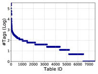
(a)

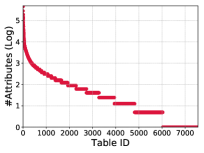
(b)

Figure 3: Distribution of (a) Tags and (b) Attributes per Table in Socrata Data Lake.

YagoCloud benchmark - To have a fair comparison with YAGO, we cannot use our real open data lakes because YAGO has low coverage over this data. Hence, we synthesis a data lake where YAGO has full coverage and therefore the class hierarchy of YAGO would be a reasonable alternative for navigation. YagoCloud is a collection of 370 tables with 2,364 attributes that can be organized using the taxonomy of YAGO. Like TagCloud benchmark, the distribution of attributes in tables and tags per table in this benchmark are created to emulate the observed characteristics of our crawl of open data portals (Figure 3). In YAGO, each entity is associated with one or more types. We consider 500 random leaf types that contain the words “agri”, “food”, or “farm” in their labels. These types are equivalent to tags. Each attribute in the benchmark is associated to exactly one tag. For each attribute of a table, we randomly sample its values from the set of entities associated to its tag. This guarantees that the attribute is about the type (tag). We tokenize the sampled entities into words and the word embeddings of these words are then used to generate the topic vectors of attributes. The number of values in an attribute is a random number between 10 and 1000. and the number of attributes per table is sampled from [1, 50] following a Zipfian distribution.

The sub-graph of the YAGO taxonomy that covers all ancestor classes of the benchmark types is considered as the taxonomy defined on benchmark attributes. This taxonomy is a connected and acyclic graph. Each class in the taxonomy is equivalent to a non-leaf state of navigation. To guarantee the inclusion property in the taxonomy, each non-leaf state consists of the tags corresponding to its descendant types. The topic vector of an interior state is generated by aggregating the topic vectors of its descendant attributes.

5.2 Experimental Set-up

Evaluation Measure

For our initial studies evaluating our design decisions and comparing our approach to three others (Yago, a simple tag-based baseline, and an Enterprise Knowledge Graph), we do not have a user. We simulate a user by reporting the success probability of finding each table in the lake. Conceptually what this means is that if a user had in mind a table that is in the lake and makes navigation decisions that favor picking states that are closest to attributes and tags of that table, we report the probability that they would find that table using our organization.

We therefore report for our experiments a measure we call success probability that considers a navigation to be successful if it finds tables with an attribute of or a similar attribute to the query’s attributes. We first define the success probability for attributes. Specifically, let $\kappa$ be a similarity measure between two attributes and let $0<\theta\leq 1$ be a similarity threshold.

Definition 6.

The success probability of an attribute $A$ is defined as

$$Success(A|\mathcal{O})=1-\prod_{A_{i}\in\mathcal{A}\wedge\kappa(A_{i},A)\geq\theta}(1-P(A_{i}|\mathcal{O}))$$ (24)

We use the Cosine similarity on the topic vectors of attributes for $\kappa$ and a threshold $\theta$ of $0.9$. Based on attribute success probabilities, we can compute table success probability as $Success(T|\mathcal{O})=1-\prod_{A\in T}(1-Success(A|\mathcal{O}))$. We report success probability for every table in the data lake sorted from lowest to highest probability on the x-axis (see Figure 4a as an example).

Implementation

Our implementation is in Python and uses scikit-learn library for creating initial organizations. Our experiments were run on a 4-core Intel Xeon 2.6 GHz server with 128 GB memory. To speed up the evaluation of an organization, we cache the similarity scores of attribute pairs as well as attribute and state pairs as states are updated during search.

5.3 Performance of Approximation

We evaluate the effectiveness and efficiency of our exact algorithm (using exact computation of discovery probabilities, not the approximation discussed in Section 4.2) on the TagCloud benchmark.

5.3.1 Effectiveness

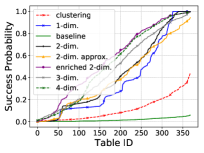
(a)

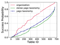
(b)

Figure 4: Success Probability of Organizations (a) on TagCloud Benchmark and (b) YagoCloud Benchmark.

We constructed the baseline organization where each attribute has as parents the tag-state of the attribute. Recall in this benchmark each attribute has a single, accurate tag. This organization is similar to the organization of open data portals. We performed an agglomerative hierarchical clustering over this baseline to create a hierarchy with branching factor 2. This organization is called clustering. Then we used our algorithm to optimize the clustering organization to create N-dimensional ($N\in\{1,2,3,4\}$) organizations (called N-dim). Figure 4a reports the success probability of each table in different organizations.

In the baseline organization, requires users to consider a large number of tags and select the best, hence the average success probability for tables in this organization is just 0.016. This clustering organization outperforms the baseline by ten times. This is because the smaller branching factor of this organization reduces the burden of choosing among so many tags as the flat organization and results in larger transition probabilities to states even along lengthy paths. Our 1-dim optimization of the clustering organization improves the success probability of the clustering organization by more than three times.

To create the N-dimensional organization ($N>1$), we clustered the tags into $N$ clusters (using $n$-medoids) and built an organization on each cluster. The 2-dim organzation has an average success probability of 0.326 which is an improvement over the baseline by 40 times. Although the number of initial tags is invariant among 1-dimensional and multi-dimensional organizations since each dimension is constructed on a smaller number of tags that are more similar, increasing the number of dimensions in an organization improves the success probability, as shown in Figure 4a.

In Figure 4a, almost 47 tables of TagCloud have very low success probability in all organizations. We observed that almost 70% of these tables contain only one attribute each of which is associated to only one tag. This makes these tables less likely to be discovered in any organization. To investigate this further, we augmented TagCloud to associate each attribute with an additional tag (the closest tag to the attribute other than its existing tag). We built a two-dimensional organization on the enriched TagCloud, which we name enriched 2-dim. This organization proves to have higher success probability overall, and improves the success probability for the least discoverable tables.

5.3.2 Efficiency

The construction time of clustering, 1-dim, 2-dim, 3-dim, 4-dim, and enriched 2-dim organizations are 0.2, 231.3, 148.9, 113.5, 112.7, 217 seconds, respectively. Note that the baseline relies on the existing tags and requires no additional construction time. Since dimensions are optimized independently and in parallel, the reported construction times of the multi-dimensional organizations indicate the time it takes to finish optimizing all dimensions.

5.3.3 Approximation

The effectiveness and efficiency numbers we have reported so far are for the non-approximate version of our algorithm. To evaluate an organization during search we only examine the states and attributes that are affected by the change an operation has made. Thus, this pruning guarantees exact computation of success probabilities. Our experiments, shown in Figure 5, indicate that although local changes can potentially propagate to the whole organization, on average less than half of states and attributes are visited and evaluated for each search iteration. Furthermore, we considered approximating discovery probabilities using a representative set size of 10% of the attributes and only evaluated those representatives that correspond to the affected attributes. This reduces the number of discovery probability evaluations to only 6% of the attributes. As shown in Figure 4a, named 2-dim approx, this approximation has negligible impact on the success probabilities of tables in the constructed organization. The construction time of 2-dim (without the approximation) is 148.9 seconds. For 2-dim approx (using a representative size of 10%) is 30.3 seconds. The remaining experiments report organizations (on much larger lakes) created using this approximation for scalability.

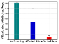
(a)

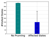
(b)

Figure 5: Pruning (a) Domains and (b) States on TagCloud Benchmark.

5.4 Comparison of Organizations

We now compare our approach with (1) a hand-curated taxonomy on the YagoCloud benchmark, (2) the flat baseline on a large real data lake Socrata, and (3) an automatically generated enterprise knowledge graph (EKG) fernandez2018aurum ; fernandez2018seeping on a smaller sample of this lake Socrata-1.

5.4.1 Comparison to A Knowledge Base Taxonomy

We compare the effectiveness of using the existing YAGO taxonomy on YagoCloud tables for navigation with our organization. Figure 4b shows the success probability of tables in the benchmark when navigating the YAGO taxonomy and our data lake organization. The taxonomy consists of 1,171 nodes and 2,274 edges while our (1-dimensional) organization consists of 442 nodes and 565 edges. Each state in the optimized organization consists of a set of types that need to be further interpreted while each state in the taxonomy refers to a YAGO class label. However, the more compact representation of topics of the attributes leads to a more effective organization for navigation. To understand the influence of taxonomy/organization size on discovery effectiveness, we condensed the taxonomy. Similar to the knowledge fragment selection approach Hellmann:2008 , we created a compact taxonomy by eliminating the immediate level of nodes above the leaves unless they have other children. This leads to a taxonomy that has 444 nodes and 1,587 edges which is closer to the size of our organization. Condensing the taxonomy increases the branching factor of nodes while decreasing the length of discovery paths. This leads to a slight decrease in success probability compared to the original taxonomy. Knowledge base taxonomies are efficient for organizing the knowledge of entities. However, our organizations are able to optimize the navigation better based on the data lake distribution.

5.4.2 Comparison to a Baseline on Real Data

We constructed ten organizations on the Socrata lake by first partitioning its tags into ten groups using k-medoids clustering kaufmann:1987 . We apply Algorithm 1 on each cluster to approximate an optimal organization. We use an agglomerative hierarchical clustering of tags in Socrata as the initial organization. In each iteration, we approximate the success probability of the organization using a representative set with a size that is 10% of the total number of attributes in the organization. Table 3 reports the number of representatives considered for this approximation in each organization along with other relevant statistics. Since the cluster sizes are skewed, the number of attributes reachable via each organization has a high variance. Recall that Socrata has just over 50K attributes and they might have multiple tags, so many are reachable in multiple organizations. It took 12 hours to construct the multi-dimensional organization.

Table 3: Statistics of 10 Organizations of Socrata Lake.

Org	#Tags	#Atts	#Tables	#Reps
1	2,031	28,248	3,284	2,824
2	1,735	11,363	1,885	1,136
3	1,648	20,172	9,792	2,017
4	1,572	19,699	2,933	1,969
5	1,378	11,196	1,947	1,119
6	1,245	17,083	1,934	1,708
7	829	8,848	1,302	884
8	353	6,816	831	681
9	240	3,834	614	383
10	43	118	33	11

Figure 6a shows the success probability of the ten organizations on the Socrata data lake. Using this organization, a table is likely to be discovered during navigation of the data lake with probability of 0.38, compared to the current state of navigation in data portals using only tags, which is 0.12. Recall that to evaluate the discovery probability of an attribute, we evaluate the probability of discovering the penultimate state that contains its tag and multiply it by the probability of selecting the attribute among the attributes associated to the tag. The distribution of attributes to tags depends on the metadata. Therefore, the organization algorithm does not have any control on the branching factor at the lowest level of the organization, which means that the optimal organization is likely to have a lower success probability than 1.

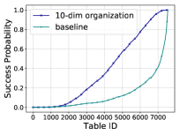
(a)

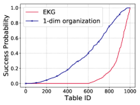
(b)

Figure 6: (a) Success Probability of Tables in Socrata Lake using Organization and Baseline. (b) Success Probability of Tables in Socrata-1 Lake using Organization and EKG.

5.4.3 Comparison to Linkage Navigation

Automatically generated linkage graphs are an alternative navigation structure to an organization. An example of a linkage graph is the Enterprise Knowledge Graph (EKG) fernandez2018aurum ; fernandez2018seeping . Unlike organizations which facilitate exploratory navigation, in EKG, navigation starts with known data. A user writes queries on the graph to find related attributes through keyword search followed by similarity queries to find other attributes similar to these attributes.

To study the differences between linkage navigation and organization navigation, we compare the probability of discovering tables using each. We used a smaller lake (Socrata-1) for this comparison because the abundance of linkages between attributes in a large data lake makes our evaluation using large EKGs computationally expensive. In the EKG, each attribute in a data lake is a node of the graph and there are edges based on node similarity. A syntactic edge means the Jaccard similarity of attribute values fernandez2018aurum is above a threshold and a semantic edge means the combined semantic and syntactic similarity of the attribute names is above a threshold fernandez2018seeping . To use EKG for navigation, we adapt Equation 1 such that the probability of a user navigating from node $m$ to an adjacent node $s$ is proportional to the similarity of $s$ to $m$ and is penalized by the branching factor of $m$. We consider the similarity of $s$ and $m$ to be the maximum of their semantic similarity and syntactic similarity. Since the navigation can start from arbitrary nodes, to compute the success probability of a table in an EKG, we consider the average success probability of a table over up to 500 runs each starting from a random node. We use the threshold $\theta=0.9$ for filtering the edges in EKG. This makes 3,989 nodes reachable from some node in the graph. The average and maximum branching factors of this EKG are 122.30 and 725, respectively. The average success probability of is 0.0056.

Figure 6b shows the success probability of navigation using an EKG and using an organization built on Socrata-1, when we limited the start nodes to be the ancestors of attributes of a table. Although the data lake organization has higher construction time (2.75 hours) than the EKG (1.3 hours), it outperforms EKG in effectiveness. The EKG is designed for discovering similar attributes to a known attribute. When EKG is used for exploration, the navigation can start from arbitrary nodes which results in long discovery paths and low success probability. Moreover, depending on the connectivity structure of an EKG, some attributes are not reachable in any navigation run (points in the left side of Figure 6b). In an EKG the number of navigation choices at each node depends on the distribution of attribute similarity. This causes some nodes to have high branching factor and leads to overall low success probability.

5.5 Effectiveness of Metadata Enrichment

The effectiveness of an organization depends on the number of tags associated to attributes. For data lakes with no or limited tags, we propose to transfer tags from another data lake that has tags. Specifically, we transfer the tags of the Socrata data lake to attributes of CKAN (which has no tags). Figure 7a shows the distribution of de-duplicated positive training samples per tag in Socrata. Despite the large number of tags (11,083), only very few of them have enough positive samples (associated attributes) for training a classifier. We considered the ratio of one to nine for positive and negative samples. We employed the distributed gradient boosting of XGBoost Chen:2016:XST to train classifiers on the tags with at least 10 positive training samples (866 tags). The training algorithm performs grid search for hyper-parameter tuning of classifiers. Figure 7b demonstrates the accuracy of the 10-fold cross validation of the classifiers with top-100 F1-scores. Out of 866 tags of Socrata, 751 were associated to CKAN attributes and a total of 7,347 attributes got at least one tag. The most popular tag is domaincategory_government. Figure 8a shows the distribution of newly associated tags to CKAN attributes for the 20 most popular tags. Figure 8b reports the success probability of a 1-dimensional organization. More than half of the tables are now searchable through the organization that were otherwise unreachable in the lake.

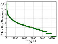
(a)

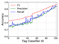
(b)

Figure 7: (a) No. Positive Training Samples and
(b) Accuracy of Tag Classifiers.

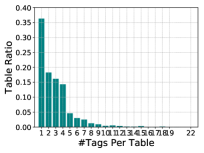
(a)

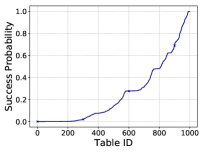
(b)

Figure 8: (a) Distribution of Tags Added to CKAN
(b) Success Prob. of CKAN after Metadata Enrichment.

5.6 User Study

We performed a formal user study to compare search by navigation to the major alternative of keyword search. Through a formal user study, we investigated how users perceive the usefulness of the two approaches.

To remain faithful to keyword search engines, we created a semantic search engine that supports keyword search over attribute values and tables metadata (including attribute names and table tags). The search engine performs query expansion with semantically similar terms. The search engine supports BM25 schutze2008introduction document search and semantic keyword search using pretrained GloVe word vectors pennington2014glove . Our implementation uses the library Xapian to perform keyword search. Users can optionally enable query expansion by augmenting the keyword query with additional semantically similar terms. We also created a prototype that enables participants to navigate our organizations. In this prototype, each node of an organization is labeled with a set of representative tags. We label leaf nodes (where attributes are located) with corresponding table names and penultimate nodes (where single tags are located) with the corresponding tags. The remaining nodes are labeled with two tags which are the first and second most occurring tags, among its children’s labels, for the nodes’ attributes. If these tags belong to the label of the same child, we choose the third most occurring tag and so on. At each state, the user can navigate to a desired child node or backtrack to the parent of the current node.

Hypotheses. The goal of our user study is to test the following hypotheses: H1) given the same amount of time, participants would be able to find as many relevant tables with navigation as with keyword search; H2) given the same amount of time, participants who use navigation would be able to find relevant tables that cannot be found by keyword search. We measure the disjointness of results with the symmetric difference of result sets normalized by the size of the union of results, i.e., for two result sets $R$ and $T$, the disjointness is computed by $1-\frac{|R\cap T|}{|R\cup T|}$.

Study Design. We considered Socrata-2 and Socrata-3 data lakes for our user study and defined an overview information need scenario for each data lake. We made sure that these scenarios are similar in difficulty by asking a number of domain experts who were familiar with the underlying data lakes to rate several candidate scenarios. Note that the statistically insignificant difference between the number of tabels found for each scenario by our participants provides evidence that our two scenarios were infact similar in difficulty. The scenario used for Socrata-2 asks participants to find tables relevant to the scenario “suppose you are a journalist and you’d like to find datasets published by governments on the topic of smart city.”. The scenario used for Socrata-3 asks participants to find tables relevant to the scenario “Suppose you are a data scientist in a medical company and you would like to find datasets about clinical research”. During the study, we asked participants to use keyword search and navigation to find a set of tables which they deemed relevant to given scenarios. For this study, we recruited 12 participants using convenience sampling EtikanMA2016 ; given2008sage . The participants have diverse backgrounds with undergraduate and graduate education in computer science, engineering, math, statistics, and management sciences.

This study was a within-subject design. In our setting, we want to avoid two potential sources of invalidity. First, participants might become familiar with the underlying data lake during the first scenario which then might help them to search better in their second scenario. To address this problem, we made sure that Socrata-2 and Socrata-3 do not have overlapping tags and tables. Second, the sequence in which the participants use the two search approaches can be the source of confounding. To mitigate for this problem, we made sure that half of the participants first performed keyword search and the rest performed navigation first. In summary, we handled the effect of these two sources of invalidity using a balanced latin square design with 4 blocks (block 1: Socrata-2/navigation first, block 2: Socrata-3/navigation first, etc.). We randomly assigned equal number of participants to each of these blocks. For each participant, the study starts with a short training session, after that, we gave the participants 20 minutes for each scenario.

Table 4: Number of Tables Found by the Search Techniques.

Participant ID	Navigation	Keyword Search
1	11	8
2	32	24
3	2	2
4	25	13
5	45	14
6	44	34
7	23	10
8	14	8
9	20	10
10	7	8
11	6	1
12	6	2

Results. Because of our small sample size, we used the non-parametric Mann-Whitney test to determine the significance of the results and tested our two-tailed hypotheses. We found that there is no statistically significant difference between the number of relevant tables found using the organization and keyword search. The number of tables found by each participant for each scenario is listed in Table 4. We first asked two collaborators to eliminate irrelevant tables found. Since the number of irrelevant data was negligible (less than 1% for both approaches) we will not further report on this process. This confirms our first hypothesis. The maximum number of tables found by navigating an organization and performing keyword search was 44 and 34, respectively. Moreover, a Mann-Whitney test indicated that the disjointness of results was greater for participants who used organization (Mdn = 0.985) than for participants who used keyword search (Mdn = 0.916), U = 612, p = 0.0019. This confirms our second hypothesis. Note that the disjointness was computed for each pair of participants who worked on the same scenario using the same approach, then the pairs generated for each technique were compared together. The calculated disjointness pairs are included in Table 5. Based on our investigation, this difference might be because participants used very similar keywords, whereas the paths which were taken by each participant while navigating an organization were very different. In other words, As some participants described, they were having a hard time finding keywords that best described their interest since they did not know what was available, whereas with our organization, at each step, they could see what seemed more interesting to them and find their way based on their preferences. As one example, for the smart city overview scenario, everyone found tables tagged with the term City using search. But using organization, some users found traffic monitoring data, while others found crime detection data, while others found renewable energy plans. Of course if they knew a priori this data was in the lake they could have formulated better keyword search queries, but navigation allowed them to conveniently discover these relevant tables without prior knowledge. One very interesting observation in this study is that although participants find similar number of tables, there is only around 5% intersection between tables found using keyword search and tables found using our approach. This suggests that organization can be a good complement to the keyword search and vice versa.

We evaluated the usability by asking each participant to fill out a standard post-experiment system usability scale (SUS) questionnaire Brooke:2013:SR:2817912.2817913 after each block. This questionnaire is designed to measure a user’s judgment of a system’s effectiveness and efficiency. We analyzed participants’ rankings, and kept record of the number of questions for which they gave a higher rankings to each approach. Our results indicate that 58% of the participants preferred to use keyword search, we suspect in part due to familiarity. No participant had neutral preference. Still having 42% prefer navigation indicates a clear role for this second, complementary modality.

Table 5: Disjointness Scores of Result Sets of Keyword Search (kw) and Navigation (nav) for each Pair of Participants.

Participant ID	1 Kw/Nav	2 Kw/Nav	3 Kw/Nav	4 Kw/Nav	5 Kw/Nav	6 Kw/Nav	7 Kw/Nav	8 Kw/Nav	9 Kw/Nav	10 Kw/Nav	11 Kw/Nav	12 Kw/Nav
1			0.733/1.000	0.714/0.937	0.916/1.000	0.875/1.000					0.947/1.000	0.800/0.928
2							1.000/1.000	1.000/1.000	1.000/1.000	1.000/1.000
3	0.733/1.000			0.850/0.960	0.941/1.000	0.923/0.966					0.850/0.985	0.850/1.000
4	0.714/0.937		0.850/0.960		1.000/1.000	0.818/1.000					0.871/0.985	0.777/0.837
5	0.916/1.000		0.941/1.000	1.000/1.000		1.000/0.833					1.000/1.000	1.000/1.000
6	0.875/1.000		0.923/0.966	0.818/1.000	1.000/0.833						0.939/0.979	0.916/0.964
7		1.000/1.000						0.913/0.969	0.892/0.930	0.935/1.000
8		1.000/1.000					0.913/0.969		0.888/1.000	0.909/1.000
9		1.000/1.000					0.892/0.930	0.888/1.000		0.875/0.969
10		1.000/1.000					0.935/1.000	0.909/1.000	0.875/0.969
11	0.947/1.000		0.850/0.985	0.871/0.985	1.000/1.000	0.939/0.979						0.952/0.901
12	0.800/0.928		0.850/1.000	0.777/0.837	1.000/1.000	0.916/0.964					0.952/0.901

6 Related Work

Entity-based Querying - While traditional search engines are built for pages and keywords, in entity search, a user formulates queries to directly describe her target entities and the result is a collection of entities that match the query Chakrabarti:2006 . An example of a query is “database #professor”, where professor is the target entity type and “database” is a descriptive keyword. Cheng et. al propose a ranking algorithm for the result of entity queries where a user’s query is described by keywords that may appear in the context of desired entities Cheng:2007 .

Data Repository Organization - Goods is Google’s specialized dataset catalog for about billions of Google’s internal datasets Halevy:2016 . The main focus of Goods is to collect and infer metadata for a large repository of datasets and make it searchable using keywords. Similarly, IBM’s LabBook provides rich collaborative metadata graphs on enterprise data lakes Labbook15 . Skluma BSCF17 also extracts metadata graphs from a file system of datasets. Many of these metadata approaches include the use of static or dynamic linkage graphs Deng+17 ; Man+18 ; fernandez2018seeping ; fernandez2018aurum , join graphs for adhoc navigation DBLP:journals/pvldb/ZhuPNM17 , or version graphs HellersteinSGSA17 . These graphs allow navigation from dataset to dataset. However, none of these approaches learn new navigation structures optimized for dataset discovery.

Taxonomy Induction - The task of taxonomy induction creates hierarchies where edges represent is-a (or subclass) relations between classes. The is-a relation represents true abstraction, not just the subset-of relation as in our approach. Moreover, taxonomic relationship between two classes exists independent of the size and distribution of the data being organized. As a result, taxonomy induction relies on ontologies or semantics extracted from text Kozareva:2010 or structured data PoundPT11 . Our work is closes to concept learning, where entities are grouped into new concepts that are themselves organized in is-a hierarchies Lehmann:2009:DLC:1577069.1755874 .

Faceted Search - Faceted search enables the exploration of entities by refining the search results based on some properties or facets. A facet consists of a predicate (e.g., model) and a set of possible terms (e.g., honda, volvo). The facets may or may not have a hierarchical relationship. Currently, most successful faceted search systems rely on term hierarchies that are either designed manually by domain experts or automatically created using methods similar to taxonomy induction zheng2013survey ; Pound:2011:FDS ; Duan:2013:SKS . The large size and dynamic nature of data lakes makes the manual creation of a hierarchy infeasible. Moreover, since values in tables may not exist in external corpora NargesianZPM18 , such taxonomy construction approaches of limited usefulness for the data lake organization problem.

Keyword Search - Google’s dataset search uses keyword search over metadata and relies on dataset owners providing rich semantic metadata DBLP:conf/www/BrickleyBN19 . As shown in our user study this can help users who know what they are looking for, but has less value in serendipitous data discovery as a user tries to better understand what data is available in a lake.

7 Conclusion and Future Work

We defined the data lake organization problem of creating an optimal organization over tables in a data lake. We proposed a probabilistic framework that models navigation in data lakes on an organization graph. We frame the data lake organization problem as an optimization problem of finding an organization that maximizes the discovery probability of tables in a data lake and proposed an efficient approximation algorithm for creating good organizations. To build an organization, we use the attributes of tables together with any tags over the tables to combine table-level and instance-level features. The effectiveness and efficiency of our system are evaluated by benchmark experiments involving synthetic and real world datasets. We have also conducted a user study where participants use our system and a keyword search engine to perform the same set of tasks. It is shown that our system offers good performance, and complements keyword search engines in data exploration. Future work includes empirically studying the scalability of our algorithm to larger data lakes, integrating keyword search and navigation as two interchangable modalities in a unified data exploration framework. Based on the feedback and comments from the user study, we strongly believe that these extensions will further improve the user’s ability to navigate in large data lakes.

References

- (1) Arenas, M., Cuenca Grau, B., Kharlamov, E., Marciuška, v., Zheleznyakov, D.: Faceted search over rdf-based knowledge graphs. Web Semantics 37, 55–74 (2016)
- (2) Beckman, P., Skluzacek, T.J., Chard, K., Foster, I.T.: Skluma: A statistical learning pipeline for taming unkempt data repositories. In: Scientific and Statistical Database Management, pp. 41:1–41:4 (2017)
- (3) Brickley, D., Burgess, M., Noy, N.F.: Google dataset search: Building a search engine for datasets in an open web ecosystem. In: WWW, pp. 1365–1375 (2019)
- (4) Brooke, J.: Sus: A retrospective. J. Usability Studies 8(2), 29–40 (2013)
- (5) Cafarella, M.J., Halevy, A.Y., Khoussainova, N.: Data integration for the relational web. PVLDB 2(1), 1090–1101 (2009)
- (6) Cafarella, M.J., Halevy, A.Y., Khoussainova, N.: Data integration for the relational web. PVLDB 2(1), 1090–1101 (2009)
- (7) Cafarella, M.J., Halevy, A.Y., Wang, D.Z., Wu, E., Zhang, Y.: Webtables: exploring the power of tables on the web. PVLDB 1(1), 538–549 (2008)
- (8) Callery, A.: Yahoo! Cataloging the Web (1996). URL misc.library.ucsb.edu/untangle/callery.html
- (9) Chakrabarti, S., Puniyani, K., Das, S.: Optimizing scoring functions and indexes for proximity search in type-annotated corpora. In: WWW, pp. 717–726 (2006)
- (10) Chen, T., Guestrin, C.: Xgboost: A scalable tree boosting system. In: SIGKDD, pp. 785–794 (2016)
- (11) Cheng, T., Yan, X., Chang, K.C.C.: Entityrank: Searching entities directly and holistically. In: VLDB, pp. 387–398 (2007)
- (12) Das Sarma, A., Fang, L., Gupta, N., Halevy, A.Y., Lee, H., Wu, F., Xin, R., Yu, C.: Finding related tables. In: SIGMOD, pp. 817–828 (2012)
- (13) Deng, D., Fernandez, R.C., Abedjan, Z., Wang, S., Stonebraker, M., Elmagarmid, A.K., Ilyas, I.F., Madden, S., Ouzzani, M., Tang, N.: The data civilizer system. In: CIDR (2017)
- (14) Duan, H., Zhai, C., Cheng, J., Gattani, A.: Supporting keyword search in product database: A probabilistic approach. PVLDB 6(14), 1786–1797 (2013)
- (15) Etikan, I., Musa, S.A., Alkassim, R.S.: Comparison of convenience sampling and purposive sampling. American Journal of Theoretical and Applied Statistics 5(1), 1–4 (2016)
- (16) Fernandez, R.C., Abedjan, Z., Koko, F., Yuan, G., Madden, S., Stonebraker, M.: Aurum: A data discovery system. In: ICDE, pp. 1001–1012. IEEE (2018)
- (17) Fernandez, R.C., Mansour, E., Qahtan, A.A., Elmagarmid, A.K., Ilyas, I.F., Madden, S., Ouzzani, M., Stonebraker, M., Tang, N.: Seeping semantics: Linking datasets using word embeddings for data discovery. In: ICDE, pp. 989–1000. IEEE (2018)
- (18) Friedman, N., Koller, D.: Being bayesian about network structure. A bayesian approach to structure discovery in bayesian networks. Machine Learning 50(1-2), 95–125 (2003)
- (19) Given, L.M. (ed.): The Sage encyclopedia of qualitative research methods. Sage Publications, Lox Angeles, Calif (2008)
- (20) Halevy, A., Korn, F., Noy, N.F., Olston, C., Polyzotis, N., Roy, S., Whang, S.E.: Goods: Organizing google’s datasets. In: SIGMOD, pp. 795–806 (2016)
- (21) Hassanzadeh, O., Ward, M.J., Rodriguez-Muro, M., Srinivas, K.: Understanding a large corpus of web tables through matching with knowledge bases: an empirical study. In: Proceedings of the 10th Int. Workshop on Ontology Matching, pp. 25–34 (2015)
- (22) Hellerstein, J.M., Sreekanti, V., Gonzalez, J.E., Dalton, J., Dey, A., Nag, S., Ramachandran, K., Arora, S., Bhattacharyya, A., Das, S., Donsky, M., Fierro, G., She, C., Steinbach, C., Subramanian, V., Sun, E.: Ground: A data context service. In: CIDR (2017)
- (23) Hellmann, S., Lehmann, J., Auer, S.: Learning of owl class descriptions on very large knowledge bases. In: ISWC, pp. 102–103 (2008)
- (24) Hulsebos, M., Hu, K.Z., Bakker, M.A., Zgraggen, E., Satyanarayan, A., Kraska, T., Demiralp, Ç., Hidalgo, C.A.: Sherlock: A deep learning approach to semantic data type detection. In: KDD, pp. 1500–1508 (2019)
- (25) Ibrahim, Y., Riedewald, M., Weikum, G.: Making sense of entities and quantities in web tables. In: CIKM, pp. 1703–1712 (2016)
- (26) Ibrahim, Y., Riedewald, M., Weikum, G., Zeinalipour-Yazti, D.: Bridging quantities in tables and text. In: ICDE, pp. 1010–1021. IEEE (2019)
- (27) Joulin, A., Grave, E., Bojanowski, P., Mikolov, T.: Bag of tricks for efficient text classification. ACL (2017)
- (28) Kandogan, E., Roth, M., Schwarz, P.M., Hui, J., Terrizzano, I.G., Christodoulakis, C., Miller, R.J.: Labbook: Metadata-driven social collaborative data analysis. In: IEEE Big Data, pp. 431–440 (2015)
- (29) Kaufmann, L., Rousseeuw, P.: Clustering by means of medoids. Data Analysis based on the L1-Norm and Related Methods (1987)
- (30) Khreich, W., Granger, E., Miri, A., Sabourin, R.: A survey of techniques for incremental learning of HMM parameters. Inf. Sci. 197, 105–130 (2012)
- (31) Koren, J., Zhang, Y., Liu, X.: Personalized interactive faceted search. In: WWW, pp. 477–486 (2008)
- (32) Kozareva, Z., Hovy, E.: A semi-supervised method to learn and construct taxonomies using the web. In: EMNLP, pp. 1110–1118 (2010)
- (33) Lehmann, J.: Dl-learner: Learning concepts in description logics. J. Mach. Learn. Res. 10, 2639–2642 (2009)
- (34) Limaye, G., Sarawagi, S., Chakrabarti, S.: Annotating and searching web tables using entities, types and relationships. PVLDB 3(1-2), 1338–1347 (2010)
- (35) Manning, C.D., Raghavan, P., Schütze, H.: Introduction to information retrieval. Cambridge University Press (2008)
- (36) Mansour, E., Deng, D., Fernandez, R.C., Qahtan, A.A., Tao, W., Abedjan, Z., Elmagarmid, A.K., Ilyas, I.F., Madden, S., Ouzzani, M., Stonebraker, M., Tang, N.: Building data civilizer pipelines with an advanced workflow engine. In: ICDE, pp. 1593–1596. IEEE (2018)
- (37) Mikolov, T., Sutskever, I., Chen, K., Corrado, G.S., Dean, J.: Distributed representations of words and phrases and their compositionality. In: NIPS, pp. 3111–3119 (2013)
- (38) Miller, R.J., Nargesian, F., Zhu, E., Christodoulakis, C., Pu, K.Q., Andritsos, P.: Making open data transparent: Data discovery on open data. IEEE Data Eng. Bull. 41(2), 59–70 (2018)
- (39) Nargesian, F., Zhu, E., Pu, K.Q., Miller, R.J.: Table union search on open data. PVLDB 11(7), 813–825 (2018)
- (40) Pennington, J., Socher, R., Manning, C.D.: Glove: Global vectors for word representation. In: EMNLP, pp. 1532–1543 (2014)
- (41) Pimplikar, R., Sarawagi, S.: Answering table queries on the web using column keywords. PVLDB 5(10), 908–919 (2012)
- (42) Pound, J., Paparizos, S., Tsaparas, P.: Facet discovery for structured web search: a query-log mining approach. In: SIGMOD, pp. 169–180 (2011)
- (43) Pound, J., Paparizos, S., Tsaparas, P.: Facet discovery for structured web search: A query-log mining approach. In: SIGMOD, pp. 169–180 (2011)
- (44) Ritze, D., Lehmberg, O., Oulabi, Y., Bizer, C.: Profiling the potential of web tables for augmenting cross-domain knowledge bases. In: WWW, pp. 251–261 (2016)
- (45) Snow, R., Jurafsky, D., Ng, A.Y.: Semantic taxonomy induction from heterogenous evidence. In: International Conference on Computational Linguistics, pp. 801–808. The Association for Computer Linguistics (2006)
- (46) Suchanek, F.M., Kasneci, G., Weikum, G.: Yago: a core of semantic knowledge. In: Proceedings of the 16th International Conference on World Wide Web, WWW 2007, Banff, Alberta, Canada, May 8-12, 2007, pp. 697–706 (2007)
- (47) Velardi, P., Faralli, S., Navigli, R.: Ontolearn reloaded: A graph-based algorithm for taxonomy induction. Computational Linguistics 39(3), 665–707 (2013)
- (48) Venetis, P., Halevy, A., Madhavan, J., Paşca, M., Shen, W., Wu, F., Miao, G., Wu, C.: Recovering semantics of tables on the web. PVLDB 4(9), 528–538 (2011)
- (49) Yang, H., Callan, J.: A metric-based framework for automatic taxonomy induction. In: International Conference on Computational Linguistics, pp. 271–279. The Association for Computer Linguistics (2009)
- (50) Yang, J., Zhang, W., Yang, S., Zhang, Y., Lin, X., Yuan, L.: Efficient set containment join. VLDB J. 27(4), 471–495 (2018)
- (51) Zheng, B., Zhang, W., Feng, X.F.B.: A survey of faceted search. Journal of Web engineering 12(1&2), 041–064 (2013)
- (52) Zhu, E., Deng, D., Nargesian, F., Miller, R.J.: JOSIE: overlap set similarity search for finding joinable tables in data lakes. In: SIGMOD, pp. 847–864 (2019)
- (53) Zhu, E., Nargesian, F., Pu, K.Q., Miller, R.J.: LSH ensemble: Internet-scale domain search. PVLDB 9(12), 1185–1196 (2016)
- (54) Zhu, E., Pu, K.Q., Nargesian, F., Miller, R.J.: Interactive navigation of open data linkages. PVLDB 10(12), 1837–1840 (2017)