An Image-based Tapered Gridded Estimator (ITGE) for the angular power spectrum

Abstract

We present the Image-based Tapered Gridded Estimator (ITGE) to measure the angular power spectrum $(C_{\ell})$ of the sky signal directly from the visibilities measured in radio-interferometric observations. The ITGE allows us to modulate the sky response through a window function which is implemented in the image plane, and it is possible to choose a wide variety of window functions. In the context of the cosmological HI 21-cm signal, this is useful for masking out the sky signal from specific directions which have strong residual foregrounds. In the context of the ISM in external galaxies, this is useful to separately estimate the $C_{\ell}$ of different parts of the galaxy. The ITGE deals with gridded data, hence it is computationally efficient. It also calculates the noise bias internally and exactly subtracts this out to give an unbiased estimate of $C_{\ell}$. We validate the ITGE using realistic VLA simulations at $1.4{\rm GHz}$. We have applied the ITGE to estimate the $C_{\ell}$ of HI 21-cm emission from different regions of the galaxy NGC 628. We find that the slope of the measured $C_{\ell}$ in the outer region is significantly different as compared with the inner region. This indicates that the statistical properties of ISM turbulence possibly differ in different regions of the galaxy.

1 Introduction

Measurements of the cosmological redshifted neutral hydrogen (HI) 21-cm power spectrum can be used to probe the Universe over a large redshift range $0<z~{}\hbox to0.0pt{$<$\hss}{\lower 4.30554pt\hbox{$\sim$}}200$ (e.g. Bharadwaj & Ali 2005; Furlanetto, Oh & Briggs. 2006; Morales & Wyithe 2010; Prichard & Loeb 2012; Mellema et al. 2013). Several ongoing experiments such as Donald C. Backer Precision Array to Probe the Epoch of Reionization (PAPER, Parsons et al. 2010), the Low Frequency Array (LOFAR, var Haarlem et al. 2013; Yatawatta et al. 2013), the Murchison Wide-field Array (MWA, Bowman et al. 2013; Tingay et al. 2013) and the Giant Metrewave Radio Telescope (GMRT, Swarup et al. 1991) are aiming to detect the 21-cm power spectrum from the Epoch of Reionization (EoR). Also, future experiment like the Square Kilometer Array (SKA1 LOW, Koopmans et al. 2015) and the Hydrogen Epoch of Reionization Array (HERA, DeBoer et al. 2017) are designed to detect the EoR 21-cm power spectrum with higher sensitivity. The major challenges for a detection of the cosmological 21-cm signal from the high redshift Universe are the astrophysical foregrounds which are 4-5 orders of magnitude brighter than the expected 21-cm signal (Shaver et al., 1999; Santos et al., 2005; Ali, Bharadwaj & Chengalur, 2008; Paciga et al., 2011; Ghosh et al., 2011a, b). Measurements of the foreground power spectrum are also interesting in their own right. The power spectrum measurement of the Galactic synchrotron emission can be used to study the distribution of cosmic ray electrons and the magnetic fields in the interstellar medium (ISM) of the Milky Way (Waelkens et al., 2009; Lazarian & Pogosyan, 2012; Iacobelli et al., 2013). There are several statistical detections of the power spectrum of the diffuse Galactic synchrotron emission at low frequencies which are relevant for the study of the EoR cosmological 21-cm signal (Bernardi et al., 2009; Ghosh et al., 2012; Iacobelli et al., 2013; Choudhuri et al., 2017a).

The power spectrum measurements of other astrophysical signals using radio interferometric observations are also interesting. The power spectrum of the continuum emission from supernova remnants (SNRs) provides information about the statistics of the density and magnetic field fluctuations in the turbulent plasma of the SNR. Roy et al. (2009) have estimated the angular power spectra of the shell-type SNR Cas A and found that this is consistent with magneto-hydrodynamic turbulence in the synchrotron emitting plasma. Measurements of the HI 21-cm power spectrum from the ISM within our Galaxy and also external galaxies allow us to probe turbulence on galactic scales. In a pioneering study, Crovisier & Dickey (1983) have estimated the Galactic HI 21-cm angular power spectrum using Westerbork observations and found a roughly scale-independent power law behaviour. Several subsequent studies of the HI 21-cm emission from our Galaxy (Green, 1993), the Small Magellanic Cloud and Large Magellanic Cloud (Stanimirovic et al., 1999; Kim et al., 2007) and other external galaxies (Begum et al., 2006; Dutta et al., 2008, 2009a, 2009b, 2009c) all find power-law power spectra, the slopes however vary across these measurements. In recent studies Dutta & Bharadwaj (2013) and Dutta et al. (2013) have estimated the HI 21-cm angular power spectrum for a sample of external galaxies from the THINGS survey and found the power law index of the power spectrum to vary in the range -1.9 to -1.5 which they interpret as arising from two-dimensional ISM turbulence spanning length-scale $1$ to $10\,{\rm kpc}$ in the plane of the galaxy’s disk. Measurements of the HI 21-cm opacity fluctuations power spectra (Deshpande, Dwarakanath, & Goss, 2000; Dhawan, Goss, & Rodríguez, 2000; Roy, Peedikakkandy, & Chengalur, 2008; Roy et al., 2012; Dutta et al., 2014) allow us to probe the turbulence in the ISM at very small length-scales ($~{}1\,{\rm pc}$ and smaller).

In this endeavour, it is important to choose a suitable estimator to reliably estimate the power spectrum from the radio-interferometric data and this is currently an active research area. Seljak (1997) has proposed an image based estimator to measure the polarization in the cosmic microwave background. The main disadvantage of this image based estimator is the deconvolution error during image reconstruction which may affect the estimated power spectrum. Liu & Tegmark (2012) have directly used the measured visibilities to estimate the power spectrum in the context of the cosmological HI 21-cm signal. Dillon et al. (2015) have introduced a new power spectrum estimation technique to reduce the error by modelling the covariance of the foreground residuals from the data itself. The CHIPS estimator developed by Trott et al. (2016) uses an inverse-covariance weighting scheme which allows to suppress the foreground contamination in the measured power spectrum. Liu et al. (2016) have developed an estimator which uses the spherical Fourier-Bessel basis to incorporate the curved sky for large fields of view. The above-mentioned estimators rely on externally modelling the noise bias which arises in power spectrum estimation and subtracting this out to get an unbiased estimate of the power spectrum. Begum et al. 2006 and Dutta et al. (2008) have used the two visibility correlation formalism to estimate the power spectrum and also excluded the self-correlation of the visibilities which is responsible for the noise bias. Foregrounds in wide-field radio-interferometric observations pose a severe problem for detecting the 21-cm power spectrum as it is extremely challenging to correctly model and subtract bright point sources from the periphery of the field of view (see Choudhuri et al. 2016a for details). Residuals point sources from the outer region of the primary beam may overwhelm the cosmological 21-cm signal (Datta et al., 2010). Ghosh et al. (2011a) showed that the point sources located at the periphery of the main lobe and the side-lobes of the primary beam create an oscillatory pattern along the frequency direction in the estimated multi-frequency angular power spectrum. Equivalently, the wide-field foregrounds reduce the EoR window by the increasing the area under the foreground wedge (Thyagarajan et al., 2013). Using wide-field foreground simulations, Pober et al. (2016) showed that it is important to correctly model and subtract these wide field foregrounds for EoR detection. Ghosh et al. (2011b) showed that the oscillations in the multi-frequency angular power spectrum could be suppressed by restricting the angular extent of the telescope’s sky response through a suitably chosen window function ${\cal W}(\theta)$. This was implemented by convolving the observed visibilities with $\tilde{w}(U)$ which is the Fourier transform of ${\cal W}(\theta)$. Choudhuri et al. (2014) and Choudhuri et al. (2016b) have introduced a visibility based estimator, namely the Tapered Gridded Estimator (TGE) for power spectrum estimation. TGE uses gridded visibilities to reduce the computation time and also internally calculates and subtracts the noise bias to give an unbiased estimate of the power spectrum. The visibilities are convolved with $\tilde{w}(U)$ at the time of griding in order to suppress the contribution from the outer regions of the telescope’s field of view. Choudhuri et al. (2016a) have used realistic GMRT simulations to demonstrate that TGE successfully suppresses the contribution from point sources located at the periphery of the telescope’s field of view and Choudhuri et al. (2017a) have used the TGE to estimate the angular power spectrum of the Galactic synchrotron radiation in two fields of the TIFR GMRT Sky Survey (TGSS) (Sirothia et al., 2014) for which the data was processed and calibrated by Intema et al. (2017).

The TGE presented in Choudhuri et al. (2014, 2016b) suppresses the contribution from the outer region of the telescope’s field of view by convolving the visibilities with $\tilde{w}(U)$ at the time of gridding. Till now, the various applications of this estimator have been restricted to situations where the sky response is tapered using a circularly symmetric Gaussian window function ${\cal W}(\theta)=exp(-\theta^{2}/\theta^{2}_{w})$ where the values of $\theta_{w}$ have been chosen so as to suppress the sky response towards the periphery of the main lobe of the primary beam pattern (Figure 1 of Choudhuri et al. 2016a). In such cases, $\tilde{w}(U)$ also is a circularly symmetric Gaussian and the extent of the convolution is restricted to a small disk in the baseline plane, the value of $\tilde{w}(U)$ becomes extremely small beyond this disk, and the contributions from the distant baselines can be neglected. The TGE proves to be a fast and reliable power spectrum estimator in such situations. However, there are situations where one would like to use a window function ${\cal W}(\vec{\theta})$ which is not a simple circularly symmetric Gaussian. In the context of the cosmological HI 21-cm power spectrum, it would be preferable to use a window function which has a value ${\cal W}(\theta)\sim 1$ over a reasonably large angular extent near the centre of the field of view and then vary rapidly fall to a value close to zero at larger angles (for example the Butterworth function used here) instead of the Gaussian which falls off gradually away from the centre. Again, it may be desirable to mask out select regions of the sky corresponding to the locations of bright sources where significant residuals persist after source subtraction (e.g. Figure 9 of Ghosh et al. 2012). In the context of the ISM, we may be interested in separately measuring the power spectrum in different parts of the galaxy. For example, the power spectrum in the star-forming region in the inner parts of the galaxy may be different as compared to that in the outer parts. In all of these cases ${\cal W}(\vec{\theta})$ ceases to be a circularly symmetric Gaussian function, and quite often we do not even have a closed-form analytic expression for $\tilde{w}(U)$. Further, the function $\tilde{w}(U)$ then covers a large extent in the baseline plane and the convolution of the visibilities is computationally expensive. In such situations, it is advantageous to directly apply the window function ${\cal W}(\vec{\theta})$ in the image plane instead of convolving the visibilities. The noise in the different image points are however correlated. The problem ”How to avoid the noise bias?” however still persists. In this paper, we have formulated an image-based Tapered Gridded Estimator (ITGE) where we replace the convolution in the visibility plane by a multiplication in the image plane. We have used the FFTW to make image making computationally fast. ITGE also calculates the noise bias internally and subtracts this out to give an unbiased estimate of the power spectrum. In this paper, we apply the ITGE to HI 21-cm data of the galaxy NGC 628 to separately estimate the angular power spectrum of the ISM in the inner and outer parts of this galaxy.

A brief outline of the paper follows. In Section 2, we present the mathematical formalism for ITGE. In Section 3, we validate this estimator using realistic simulations. In Section 4, we present an application of this estimator to determine the angular power spectrum of the galaxy NGC 628. Finally, we summarize and conclude in Section 5.

2 Mathematical formulation of the Image Based Tapered Gridded Estimator

In this section, we present the mathematical formalism leading to the ITGE. Here, we adopt a notation to represent the transformation between the visibilities in the baseline plane and the image on the sky plane. We deal with gridded data throughout, and these transformations are discrete Fourier transforms which can be implemented using either DFT or FFT. In our notation, the value of a quantity $L$ at the grid point $a$ on the image plane is denoted as $L_{a}$, and the corresponding quantity $Q$ at the grid point $g$ on the baseline plane is denoted as $Q_{g}$. We denote the forward and backward Fourier transform between $L$ and $Q$ as $Q_{g}=\mathcal{F}[L_{a}]$ and $L_{a}=\mathcal{I}[Q_{g}]$ respectively. Further, here we restrict our discussion to single frequency observations for simplicity.

The basic idea of ITGE is the same as that of the visibility based TGE where the estimator ${\hat{E}}_{g}$ at the grid point $g$ in the baseline plane is defined through

$${\hat{E}}_{g}=M_{g}^{-1}\,\left(\mid\mathcal{V}_{cg}\mid^{2}-\sum_{i}\mid\tilde{w}({\bf U}_{g}-{\bf U}_{i})\mid^{2}\mid\mathcal{V}_{i}\mid^{2}\right)\,.$$ (1)

as given in eqn. (17) of Choudhuri et al. (2016b). The expectation value of the estimator with respect to different random realizations of the visibility signal gives an unbiased estimate of the angular power spectrum $C_{\ell_{g}}$ at the angular multipole $\ell_{g}=2\pi U_{g}$ corresponding to the baseline ${\bf U}_{g}$. Here $M_{g}$ is a normalization factor, $\mathcal{V}_{i}$ is the visibility measured at the baseline ${\bf U}_{i}$ and $\mathcal{V}_{cg}$ represents the convolved visibilities which is evaluated at the grid point $g$ using

$$\mathcal{V}_{cg}=\sum_{i}\tilde{w}({\bf U}_{g}-{\bf U}_{i})\,\mathcal{V}_{i}\,.$$ (2)

As mentioned earlier, this convolution effectively multiplies the telescope’s sky response with the window function ${\cal W}(\vec{\theta})$ resulting in a tapered field of view. It is possible to directly estimate the power spectrum using $M_{g}^{-1}\,\left(\mid\mathcal{V}_{cg}\mid^{2}\right)$, however the self-correlation of the individual visibilities introduces a positive noise bias in the estimated power spectrum. The second term in eqn. (1) - $\sum_{i}\mid\tilde{w}({\bf U}_{g}-{\bf U}_{i})\mid^{2}\mid\mathcal{V}_{i}\mid^{2}$ evaluates the contribution from this self-correlation and subtracts this out to give an unbiased estimate of the angular power spectrum. Some signal also is lost, however, this is expected to be small when the number of visibilities at each grid point is large. The value of the normalization factor $M_{g},$ at each grid point, depends on the actual baseline distribution, the antenna primary beam pattern and the tapering window function. As discussed in Choudhuri et al. (2016b), we simulate the visibilities for a unit angular power spectrum (UAPS) $(C_{\ell}=1)$ sky signal and use these to estimate the values of $M_{g}$.

We now discuss how we have implemented eqn. (1) in the image domain. We proceed by first gridding the visibilities using

$$\mathcal{V}_{g}=\sum_{i}\Theta\left(1-\frac{\mid{\bf U}_{g}-{\bf U}_{i}\mid}{(\Delta U/2)}\right)\mathcal{V}_{i}c_{i}.$$ (3)

Here $\Theta({\bf U})$ is the Heaviside step function, $\Delta{\bf U}$ denotes the baseline grid spacing which has been chosen to be sufficiently small so that the angular scale $(\Delta U)^{-1}$, which is the extent of the dirty image, is much larger than the telescope’s field of view. In this paper, we choose $\Delta U=0.2D/\lambda$ which corresponds to an image of dimension $5$ times the telescope’s field of view. Here $c_{i}$ is a weighting function whose value we have the freedom to choose. There are two common choices of the weighting function on a grid: (a) the natural weighting which gives a constant weight $c_{i}=1$ to all the visibilities, and (b) the uniform weighting which gives a weight $c_{i}=1/N_{g}$ which is inversely proportional to the sampling density i.e. the number of visibilities $N_{g}$ at a particular grid point $g$. The choice of weighting scheme introduces differences in the resulting image, and details of possible weighting schemes are discussed in Thompson, Moran & Swenson (1986). Here we have used $c_{i}$=1 i.e. the natural weighting throughout the paper. We use the gridded visibilities to calculate the dirty image $I_{a}$ using

$$I_{a}=\mathcal{I}[\mathcal{V}_{g}],$$ (4)

and determine the convolved visibilities $\mathcal{V}_{cg}$ using

$$\mathcal{V}_{cg}=\mathcal{F}[{\cal W}_{a}I_{a}]\,.$$ (5)

Here ${\cal W}(\vec{\theta})$ is the window function that we wish to implement on the sky, and it is not restricted to be a circularly symmetric Gaussian function.

The issue now is to estimate the contribution from the visibility self-correlation using operations in the image plane. We proceed by first gridding the visibility self-correlation using

$$VSQ_{g}=\sum_{i}\Theta\left(1-\frac{\mid{\bf U}_{g}-{\bf U}_{i}\mid}{(\Delta{\bf U}/2)}\right)\mid\mathcal{V}_{i}\mid^{2}c_{i}^{2}.$$ (6)

We now consider $\tilde{w}_{g}={\cal F}[{\cal W}_{a}]$ which is the Fourier transform of the window function ${\cal W}(\vec{\theta})$, and construct the images of $\mid\tilde{w}({\bf U})\mid^{2}$ and the visibility self-correlation (eqn. 6) using

$$WSQ_{a}=\mathcal{I}\left[\mid\tilde{w}_{g}\mid^{2}\right]$$ (7)

and

$$ISQ_{a}=\mathcal{I}\left[VSQ{g}\right]$$ (8)

respectively. It is possible to obtain the second term in eqn (1) by taking the Fourier transform of the product of the two images $WSQ$ and $ISQ$ i.e.

$$\sum\limits_{i}\mid\tilde{w}({\bf U}_{g}-{\bf U}_{i})\mid^{2}\mid\mathcal{V}_{i}\mid^{2}=\mathcal{F}\left[ISQ_{a}\,WSQ_{a}\right].$$ (9)

We have used eqns. (5) and (9) in eqn. (1) to define the ITGE. As for the TGE, we have used UAPS simulations to estimate the normalization factor $M_{g}$. The values of the angular power spectrum estimated at different grid points are binned to increase the signal to noise ratio and for convenience of displaying and interpretation. Considering annular bin labeled using $a$, we have the binned ITGE defined as

$$\hat{E}(a)=\frac{\sum\limits_{g}a_{g}\hat{E}_{g}}{\sum\limits_{g}a_{g}}$$ (10)

where $a_{g}$ is the weight assigned to any particular grid point. This provides an estimate of the bin averaged angular power spectrum $\langle\hat{E}(a)\rangle=C_{\ell_{a}}$ at the mean angular multipole

$$\ell_{a}=\frac{\sum\limits_{g}a_{g}\ell_{g}}{\sum\limits_{g}a_{g}}\,.$$ (11)

Here we have evaluated the angular power spectrum in equally spaced logarithmic bins, and assigned equal weights to all the grid points i.e, $a_{g}=1$.

3 Validation

We first describe the simulation of radio interferometric visibilities which we have used to validate the ITGE. To simulate the sky signal we follow the same procedure as described in (Choudhuri et al., 2014, 2017b). Here, we use a model angular power spectrum

$$C^{M}_{\ell}=A\times\left(\frac{1000}{\ell}\right)^{\beta},$$ (12)

where $A=3\times 10^{5}$ and we choose the value of the power-law index $\beta=1.88$, this choice of values is guided by the measured $C_{\ell}$ for the galaxy NGC 628 which we analyze in the next Section. We generate the Fourier components of the temperature fluctuations on a two-dimensional grid using this model angular power spectrum and then use the FFTW to generate the temperature fluctuations $\delta T(\vec{\theta})$ on the sky plane. The total number of grid points used in this simulation are $1024\times 1024$ with an angular resolution $0.045^{{}^{\prime}}$. The flat-sky approximation is valid for a region of size $\sim 46^{{}^{\prime}}$ considered here. We use the baseline configuration of VLA antennas at $1.4\ {\rm GHz}$ pointed towards the direction of the galaxy NGC 628 (R.A.=$01{\rm h}\,36{\rm m}\,41{\rm s}$ Dec=$15^{\circ}\,47^{{}^{\prime}}\,00^{{}^{\prime\prime}}$) to simulate the visibilities. We first multiply the simulated $\delta T(\vec{\theta})$ with the VLA primary beam pattern and then use 2-D FFTW to calculate the visibilities on a baseline grid. These gridded values were interpolated to calculate the visibilities along the simulated baseline $uv$ tracks. Details of similar simulations have been discussed in (Choudhuri et al., 2017b).

To validate the estimator ITGE, we choose different types of window functions as shown in Figure 1. We first consider a Gaussian window

$${\cal W}_{G}(\vec{\theta})=\exp[-\theta^{2}/\theta^{2}_{g}]$$ (13)

with $\theta_{g}=9^{{}^{\prime}}$ as shown by the red solid curve in Figure 1. The half width half maxima (HWHM) of this Gaussian window is $\theta_{HWHM}=\sqrt{\ln 2}\,\theta_{g}=7.5^{{}^{\prime}}$. We also consider the Butterworth (BW) window given by

$${\cal W}_{BW}(\vec{\theta})=\frac{1}{1+({\theta}/{\theta_{b}})^{2N}}$$ (14)

Here $\theta_{b}$ is the HWHM of the BW window function, and we choose this to be $\theta_{b}=7.5^{{}^{\prime}}$ which is the same as that of the Gaussian. The index $N$ determines how sharply the window falls as a function of the angular distance $\theta$. Figure 1 shows the shape of the BW window for different values of $N~{}(=2,4$ and $256)$. We see that compared to the Gaussian, the BW window is flatter in the central region and falls off more sharply at large angles beyond the HWHM. Further, the BW window function falls more sharply as the value of $N$ is increased.

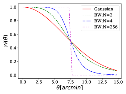
Figure 1: This shows the different window functions (Gaussian and Butterworth (BW)) used in our analysis. All of the window function have a HWHM of $7.5^{{}^{\prime}}$

We apply the ITGE to the simulated visibilities to measure the angular power spectrum considering all the window functions shown in Figure 1. Figure 2 shows the mean estimated $C_{\ell}$ and the rms. fluctuation $\sigma$ calculated using $1000$ independent realizations of the simulated data. The estimated $\sigma$ will increase if we reduce the width of the window function. This is due to the fact that the smaller window reduces the sky response, effectively causing large cosmic variance. In comparison, the HWHM of all the windows shown in Figure 1 are the same, and we expect the cosmic variance to be quite similar for these windows. Here we use $20$ equally spaced logarithmic bins in the $\ell$ range from $3\times 10^{3}$ to $3\times 10^{5}$ to increase the signal to noise ratio in the estimated $C_{\ell}$ values. The left panels show the results for the Gaussian tapering window. The upper left panel shows the estimated $C_{\ell}$ with $1-\sigma$ error bars (blue solid circles). We also show the input model $C^{M}_{\ell}$ (eqn. 12) with a red solid line for comparison. We see that the estimated values are in reasonably good agreement with the model for $\ell\geq 3\times 10^{3}$, the tapering due to the primary beam pattern and the window function modifies the shape of the estimated power spectrum at $\ell<3\times 10^{3}$ (Choudhuri et al., 2014), and we have not shown this range in these figures. We also fit the estimated $C_{\ell}$ with a power law (eq. 12) to see the efficacy of the estimator and the best fit value of the parameter $\beta$ is $1.87\pm 0.002$ which is close to the input model $(\beta=1.88)$ used for the simulations . Table  1 summarizes the recovered $\beta$ for all the window functions used in this work. The lower left panel shows $\delta=(C_{\ell}-C^{M}_{\ell})/C^{M}_{\ell}$ which is the fractional deviation between the estimated $C_{\ell}$ and the input model $C^{M}_{\ell}$. We see that the fractional deviation is less than $10\%$ for all $\ell$ values in the range $\ell\geq 3\times 10^{3}$. The shaded region in the lower panel shows the expected statistical fluctuations $\sigma/C^{M}_{\ell}$. We see that the fractional deviation $\delta$ is within $1-\sigma$ statistical fluctuations for the whole $\ell$ range $3\times 10^{3}\leq\ell\leq 3\times 10^{5}$ considered here.

	Model	Gaussian	BW,N=2	BW,N=4	BW,N=256	Annulus	Mask
$\beta$	$1.88$	$1.87\pm 0.002$	$1.87\pm 0.002$	$1.87\pm 0.003$	Not recovered	$1.87\pm 0.007$	$1.87\pm 0.01$

Table 1: This shows the recovered $\beta$ for the different window functions used in this work. Here we have used $\beta=1.88$ as the input model to simulate the sky. For the BW window with $N=256$ the estimated $C_{\ell}$ shows considerable deviations from a power law.

The right panels of Figure 2 show the results for the BW windows. Here we use $N=2,4$ and $256$ for which the shape of the window functions are shown in Figure 1. The upper right panel shows the estimated $C_{\ell}$ with $1-\sigma$ error bar for $N=2$ (green circles), $4$ (blue upper triangles) and $256$ (magenta lower triangles). We also show $C^{M}_{\ell}$ with a red solid line for comparison. For $N=4$, we have scaled the values of the estimated $C_{\ell}$ and also $C^{M}_{\ell}$ for clarity of presentation. We see that for $N=2$ and $4$ the estimated $C_{\ell}$ matches quite well with the model for the whole $\ell$ range. For $N=256$, the estimated $C_{\ell}$ deviates significantly from $C^{M}_{\ell}$ at large $\ell$ values, and we are able to recover $C^{M}_{\ell}$ within a limited $\ell$ range $3\times 10^{3}\leq\ell\leq 2\times 10^{4}$. In this case ($N=256$) the window function falls sharply at $\theta=7.5^{{}^{\prime}}$ (the HWHM, Figure 1) which introduces oscillations in the Fourier domain. The large deviations in the estimated $C_{\ell}$ are possibly a consequence of these oscillations, and we subsequently restrict the value of $N$ to $2$ and $4$ where the window function does not fall so sharply. We also fit the estimated $C_{\ell}$ for $N=2$ and $4$ with a power law and the best fit values of $\beta$ are shown in Table  1. The lower right panel shows the fractional deviation $\delta$ for the BW windows. Like for the Gaussian window, the deviations $\delta$ are consistent with the $1-\sigma$ statistical fluctuations for BW windows with $N=2$ and $4$. We note that the values of $\delta$ are less than $10\,\%$ for the whole range considered here.

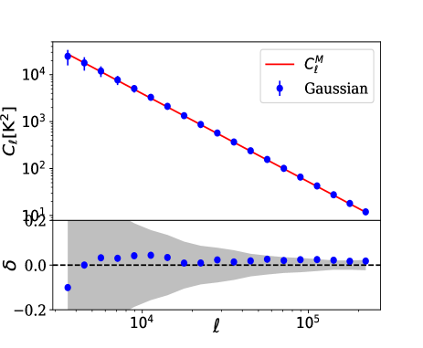
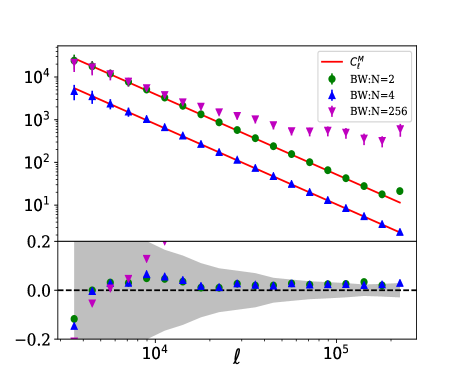
Figure 2: The left and right panels show the results for the Gaussian and the Butterworth tapering windows respectively. The upper panels show the estimated $C_{\ell}$ with $1-\sigma$ error bars. We also show the model $C^{M}_{\ell}$ with red solid line for comparison. The lower panels show the fractional deviation $(\delta)$ between the estimated $C_{\ell}$ and model $C^{M}_{\ell}$. The shaded region in the lower panels show the expected statistical fluctuations $\sigma/C^{M}_{\ell}$. In the right panel we use different color for different BW windows: $N=2$ (green circles), 4 (blue upper triangles) and 256 (magenda lower triangles). For $N=4$, we have scales the values of the estimated $C_{\ell}$ and also the model $C^{M}_{\ell}$ for clarity of presentation in the right upper panel.

The ITGE allows us to select particular regions of the image during $C_{\ell}$ estimation by choosing a suitable window function. The extent of the window function $\tilde{w}({\bf U})$ in Fourier space introduces a correlation between the power spectrum estimates at different $\ell$ bins. This could be particularly important when the bin spacing is smaller than the extent of the window function. To quantify this we have calculated the error covariance $C_{ij}=\langle\delta P_{i}\,\delta P_{j}\rangle$ of the power spectrum in the $i$ and $j$-th bins. We use the correlation coefficient $r_{ij}=C_{ij}/(\sigma_{i}\sigma_{j})$ where $\sigma^{2}_{i}$ and $\sigma^{2}_{j}$ are the error variance of the estimated power spectrum in the $i$ and $j$-th bins respectively. As mentioned earlier, the variance and covariance were estimated using $1,000$ independent realizations of the simulations. Figure 3 shows $r_{ij}$ for the Gaussian window function (left panel) and the BW window function (right panel) with $N=4$ which we have used in the subsequent analysis. We see that in both cases there is some correlation $(r_{ij}\sim 0.5)$ between the two adjacent bins (one on each side) at small $\ell$ $(\leq 9\times 10^{3})$, whereas the $\ell$-bins are all uncorrelated at larger $\ell$ where $\mid r_{ij}\mid$ has values $\sim 0.1$ or smaller. This is consistent with the fact that the window has a width of $~{}7.5^{{}^{\prime}}$ in the image plane. This has an extent in Fourier space which corresponds to $\Delta\ell\simeq 3,000$.

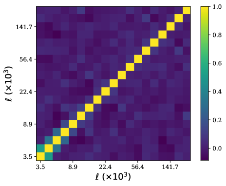
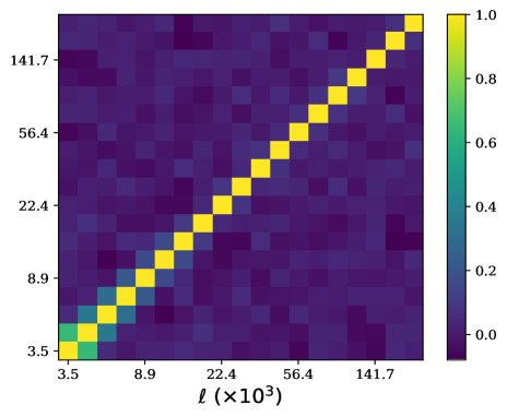
Figure 3: The left and right panels show the correlation coefficient, $r_{ij}$ between different $\ell$-bins for the Gaussian and the BW (N=4) window functions respectively. The correlation properties for both these windows are quite similar. At low $\ell$ $(\leq 9\times 10^{3})$ the two adjacent bins show correlation $r_{ij}\sim 0.5$. The correlation is small ($\mid r_{ij}\mid\sim 0.1$ or smaller) elsewhere.

We have also validated the estimator for two other window functions namely (a) the Annulus window, and (b) the Mask window. The Annulus window, shown in the left panel of Figure 4, allows us to estimate $C_{\ell}$ only from the outer annular region. The Annulus window considered here is a combination of two $N=4$ BW windows, an inner window with HWHM radius $3.5^{{}^{\prime}}$ and outer window with HWHM $7.5^{{}^{\prime}}$, and only the annular region between the two windows is used for the analysis. The Mask window, shown in the middle panel of the figure, has a $N=4$ BW window with $\theta_{b}=7.5^{{}^{\prime}}$. In addition to this, three $N=4$ BW windows with $\theta_{b}=2^{{}^{\prime}}$ have been used to mask the radiation from three specific directions. The upper right panel of the figure shows the estimated $C_{\ell}$ along with the input model $C^{M}_{\ell}$. The results have been arbitrarily scaled for clarity of presentation. The lower right panel compares the fractional deviation $\delta$ with the statistical fluctuations shown by the shaded region. We see that for both the window functions the estimated $C_{\ell}$ is largely in agreement with the model $C^{M}_{\ell}$ for the whole $\ell$ range. Again, we fit the estimated $C_{\ell}$ with a power law and the best fit values of $\beta$ are $1.87\pm 0.007$ and $1.87\pm 0.01$ for the Annulus and the Mask windows respectively (Table  1). The fractional deviation is less than $15\,\%$ for these windows. The fractional deviation $\delta$ is also consistent with the statistical fluctuations $(\sigma/C^{M}_{\ell})$ which is shown by the shaded region in the right lower panel.

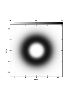
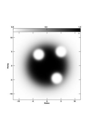
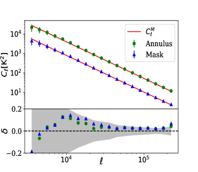
Figure 4: The left panel shows the Annulus window with inner HWHM radius $3.5^{{}^{\prime}}$ and outer HWHM radius $7.5^{{}^{\prime}}$. The middle panel shows the Mask window where we place three masks with angular HWHM radius $2^{{}^{\prime}}$ at different locations on top of the BW window which has $\theta_{b}=7.5^{{}^{\prime}}$. In both cases we use $N=4$ for the BW window. The right panel shows the same as Figure 2 but for the Annulus and Mask windows.

The Mask and the Annulus window functions have smaller angular features as compared to the BW window and we expect a larger correlation between different $\ell$-bins. Here also we have studied these correlations using $1,000$ independent realizations of the simulations. The left and right panels of Figure 5 respectively show the correlation coefficients $(r_{ij})$ for the bins centered at $\ell=6\times 10^{3}$ and $\ell=5\times 10^{4}$ with all the other $\ell$-bins. In addition to the Mask and Annulus windows, for comparison, the results are shown for the BW window with $N=4$. For all three windows, in the left panel $(\ell<9\times 10^{3})$ we find that the two adjacent bins show correlations. For the Annulus window, one further bin $(\ell=7.1\times 10^{3})$ shows a correlation of around $r_{ij}\sim 0.2$, the correlation coefficient is small $\mid r_{ij}\mid\leq 0.1$ for all the other bins in the left panel. Further, in the right panel the correlation with all the other bins has values $\mid r_{ij}\mid\leq 0.1$. We see that the Annulus and Mask window functions do introduce some correlations. Like the Gaussian and BW window with $N=4$, the effect is restricted to adjacent $\ell$-bins and low $\ell$ values $(\ell\leq 9\times 10^{3})$.

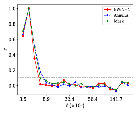
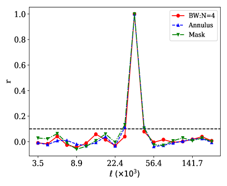
Figure 5: This shows the correlation coefficient $(r_{ij})$ for three different window functions as indicated in the figure. The left and right panels respectively show the correlation between the bins centered at $\ell=6\times 10^{3}$ and $5\times 10^{4}$ with all the other $\ell$ bins. The horizontal dashed line shows the value $r_{ij}=0.1$.

4 NGC 628 Data

Walter et al. (2008) have observed the HI emission from 34 spiral galaxies using B, C and D array configurations of the Very Large Array (VLA) as a part of The HI Nearby Galaxy Survey (THINGS). For our analysis, we use the interferometric HI data of the galaxy NGC 628 from THINGS. NGC 628 is an almost face-on spiral galaxy with an average inclination angle of $15^{\circ}$ at a distance of $7.3$ Mpc (de Blok et al., 2008). The HI extent of the galaxy is $22.0^{{}^{\prime}}\times 20.0^{{}^{\prime}}$. We use the interferometric data with the primary calibration from the THINGS archive and use the Astronomical Image Processing System (AIPS) for further analysis. We model the synchrotron continuum of the galaxy using visibilities from the channels without HI emission and make a continuum image. We perform a few rounds of self-calibration to improve the signal to noise ratio in the continuum image, and then do a continuum subtraction using the AIPS task UVSUB to retain only the HI emission in the visibilities for further analysis. Figure 6 shows the moment0 HI map of the galaxy NGC 628.

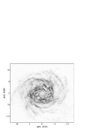
Figure 6: This shows the moment0 HI map of the galaxy NGC 628 using data from the THINGS survey.

We apply ITGE to estimate $C_{\ell}$ for the galaxy NGC 628. Figure 7 shows the measured $C_{\ell}$ with $1-\sigma$ error bars for the different windows mentioned in the previous section. The left panel shows the results for a BW window with $\theta_{b}=\theta_{HWHM}=7.5^{{}^{\prime}}$ and $N=4$. This selects nearly the entire region of the galaxy whose HI extent is approximately $20^{{}^{\prime}}$. The measured $C_{\ell}$ and the r.m.s. fluctuations $\sigma$ are shown with blue points. We have used simulations (as discussed in Section 3) to estimate $\sigma$ which is the r.m.s. fluctuation of the estimated $C_{\ell}$. These simulations differ from those in Section 3 in that the HI signal does not fill the entire sky but is restricted to a finite angular extent corresponding to that of the galaxy. We have incorporated this by multiplying the sky image with a window which roughly mimics the galaxy’s radial profile, the simulated visibilities were calculated using the resulting image. We also add a Gaussian random noise with standard deviation $\sigma_{n}=1.03\,{\rm Jy}$ to each visibility in order to account for the system noise. The value of $\sigma_{n}$ is calculated using the rms. of the actual measured VLA visibilities considering the large baselines which are likely to be noise dominated, and we have used $128$ independent realizations of the simulations to estimate $\sigma$.

Considering the estimated $C_{\ell}$, we identify a region in $\ell$-space where $C_{\ell}$ is likely to be dominated by the galaxy’s HI signal and fit a power law (eqn. 12) to the measured values. The $\ell$ range we used for fitting is $6\times 10^{3}\leq\ell\leq 6\times 10^{4}$. At smaller $\ell$ values the measured $C_{\ell}$ is affected by the finite angular extent of the galaxy and the window function whereas the system noise becomes large at the larger $\ell$ values beyond this range. The best fit values for $A$ and $\beta$ are $(3\pm 0.3)\times 10^{5}$ and $1.7\pm 0.04$. We have used values of $A$ and $\beta$ close to these best-fitted values to simulate the sky for the validation of ITGE in Section 3. The best fit model is shown with a red solid line in the left panel of Figure 7. The measured $\beta$ is roughly consistent with the earlier measurement by Dutta et al. (2013) where they obtained $\beta=1.6\pm 0.1$. As discussed in Dutta et al. (2013), we can interpret this power-law nature of the $C_{\ell}$ is due to the two-dimensional ISM turbulence in the plane of galaxy’s disk.

The middle panel of Figure 7 shows the estimated $C_{\ell}$ for a smaller BW window of width $\theta_{b}=3.5^{{}^{\prime}}$ and we use the same value of $N=4$ as earlier. Here, the window blocks out the outer parts of the galaxy, and we concentrate only the central part of the galaxy. As the width of the window is smaller here, the effect of the convolution extends upto $\ell\sim 10^{4}$. In this case we use the $\ell$-range $10^{4}\leq\ell\leq 6\times 10^{4}$ to fit the measured $C_{\ell}$. The best fit values of the parameters are $A=(3\pm 1)\times 10^{5}$ and $\beta=1.55\pm 0.1$.

The right panel of Figure 7 shows the estimated $C_{\ell}$ for the Annulus window with inner HWHM radius $3.5^{{}^{\prime}}$ and outer HWHM radius $7.5^{{}^{\prime}}$. Here our aim is to measure the HI signal from only the outer region of the galaxy. In this case the best fit value of the parameters are $A=(6\pm 0.9)\times 10^{5}$ and $\beta=2.0\pm 0.06$. Here we see a difference in the power law index between the inner part and the outer parts of the galaxy. This signifies that the statistical properties of the HI fluctuations are different in the central part of the galaxy where star formation is taking place as compared to the outer parts. We plan to investigate this issue in more detail using higher sensitivity data of the same galaxy as well as repeating a similar analysis for other galaxies.

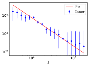
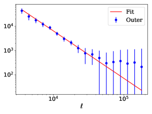
Figure 7: This shows the measured $C_{\ell}$ with $1-\sigma$ error bars for the galaxy NGC 628. The left panel is for a BW window with $\theta_{b}=7.5^{{}^{\prime}}$ which approximately corresponds to the entire extent of the galaxy. Here, the blue points are the measured values and the red solid line shows the best fit model in the range $6\times 10^{3}\leq\ell\leq 6\times 10^{4}$ (for middle panel $10^{4}\leq\ell\leq 6\times 10^{4}$). The middle panel shows the same but for a different value of $\theta_{b}=3.5^{{}^{\prime}}$ which corresponds to the inner region of the galaxy. The right panel is for the Annulus window with inner HWHM radius $3.5^{{}^{\prime}}$ and outer HWHM radius $7.5^{{}^{\prime}}$ (window shown in the left panel of Figure 4) which corresponds to the outer region of the galaxy. In all three cases, we use the value of $N=4$.

5 Summary and conclusions

It is often useful to taper the sky response when estimating the power spectrum of the diffuse sky signal directly from the visibilities measured in radio interferometric observations. In some contexts, it may also be desirable to mask out the sky signal from certain directions in order to restrict the analysis to select regions of the sky. For example, we may wish to avoid certain regions of the sky which are contaminated by strong foreground residuals, or we may be interested in studying the power spectrum of the signal from just the outer parts of a galaxy. In this paper, we introduce the Imaged based Tapered Gridded Estimator (ITGE) for estimating the power spectrum directly from the measured visibilities. Here it is possible to modulate the sky response through a window function which is implemented in the image domain on the sky plane, and it is possible to implement a wide variety of window functions in contrast to an earlier version which was purely visibility based (Choudhuri et al., 2016b). The ITGE deals with gridded data (both visibility and image) and therefore is computationally efficient. The ITGE has an added feature that it internally estimates the system noise contribution and exactly subtracts this out thereby providing an unbiased estimate of the power spectrum.

We have validated the ITGE using realistic $1.4{\rm GHz}$ simulations of VLA observations at a single frequency considering a power law input model angular power spectrum. We have considered a variety of window functions (e.g. the Gaussian, Butterworth (BW), Annulus and Mask windows) and we show that we are able to recover the input model angular power spectrum quite accurately for all of the window functions that we have considered except one BW window with $N=256$ for which the window function falls very sharply beyond the HWHM (Figure 1). However, the BW window with $N=2,4$ where there is a more gradual decline beyond the HWHM is found to work quite well. We conclude that the ITGE is able to faithfully quantify the angular power spectrum over a $\ell$ range which depends on the angular extent of the window provided that the window function does not have any very sharp features. We have also studied the error covariace between different $\ell$ bins and found that there is some correlation $(r_{ij}\sim 0.5)$ between the adjacent bins at small $\ell$ $(\leq 9\times 10^{3})$, whereas the $\ell$-bins are all uncorrelated at larger $\ell$ where $\mid r_{ij}\mid$ has values $\sim 0.1$ or smaller.

We have applied the ITGE to estimate the angular power spectrum $C_{\ell}$ of the HI 21-cm emission from the galaxy NGC 628. We have carried out the analysis using three different windows; the first two restrict the sky response to discs of HWHM radius $7.5^{{}^{\prime}}$ and $3.5^{{}^{\prime}}$ which respectively correspond to the entire extent and the inner region of the galaxy. The third window restricts the sky response to the annulus bounded by the two discs mentioned above, and this essentially quantifies the power spectrum of the HI emission from the outer parts of the galaxy. For all the cases we identify the $\ell$ range which is likely to be dominated by the galactic HI and where we expect ITGE to faithfully quantify the angular power spectrum, and we fit a power law to the $C_{\ell}$ measured in this range. We find that the best fit values of the power law index has values $\beta=1.7\pm 0.04$ and $\beta=1.55\pm 0.1$ for the entire galaxy and the inner region respectively, both of which are consistent with an earlier measurement of the angular power spectrum of the entire galaxy (Dutta et al., 2013) who find $\beta=1.6\pm 0.1$ and interpret this as arising from two-dimensional turbulence in the plane of the galaxy. The slope in the outer region of the galaxy is however found to be $\beta=2.0\pm 0.06$ which is significantly different. This signifies that the statistical properties of the HI fluctuations in the outer region of the galaxy are possibly different from those at the central part of the galaxy where star formation is taking place. We plan to investigate this issue using higher sensitivity data as well carry out a similar analysis for other galaxies in future.

Further, the entire analysis here is restricted to a single frequency. It is quite straight-forward to extend this to multi-frequency data through the multi-frequency angular power spectrum $C_{\ell}(\Delta\nu)$ (MAPS:Datta et al. (2007)) or equivalently the 3D power spectrum $P(\vec{k})$ (e.g. Choudhuri et al. 2016b ). We plan to address these issues in future work.

6 Acknowledgements

We thank an anonymous referee for helpful comments. SC acknowledge NCRA-TIFR for providing financial support. We acknowledge the THINGS collaboration for providing the data for galaxy NGC 628.

References

- Ali, Bharadwaj & Chengalur (2008) Ali S. S., Bharadwaj S.,& Chengalur J. N., 2008, MNRAS, 385, 2166A
- Begum et al. (2006) Begum, A., Chengalur, J. N., & Bhardwaj, S. 2006, MNRAS, 372, L33
- Bernardi et al. (2009) Bernardi, G., de Bruyn, A. G., Brentjens, M. A., et al. 2009, A & A, 500, 965
- Bharadwaj & Ali (2005) Bharadwaj S. , & Ali S. S. 2005, MNRAS, 356, 1519
- Bowman et al. (2013) Bowman J. D. et al., 2013, PASA, 30, e031
- Choudhuri et al. (2014) Choudhuri, S., Bharadwaj, S., Ghosh, A., & Ali, S. S., 2014, MNRAS, 445, 4351
- Choudhuri et al. (2016a) Choudhuri, S., Bharadwaj, S., Roy, N., Ghosh, A., & Ali, S. S. 2016a, MNRAS, 459, 151
- Choudhuri et al. (2016b) Choudhuri, S., Bharadwaj, S., Chatterjee, S., Ali, S. S., Roy, N., Ghosh, A., 2016b, MNRAS, 463, 4093
- Choudhuri et al. (2017a) Choudhuri, S., Bharadwaj, S., Ali, S. S., et al. 2017a, MNRAS, 470, L11
- Choudhuri et al. (2017b) Choudhuri, S., Roy, N., Bharadwaj, S., et al. 2017b, New Astronomy, 57, 94
- Crovisier & Dickey (1983) Crovisier, J., & Dickey, J. M. 1983, A & A, 122, 282
- Datta et al. (2010) Datta, A., Bowman, J. D., & Carilli, C. L. 2010, ApJ, 724, 526
- Datta et al. (2007) Datta, K. K., Choudhury, T. R., & Bharadwaj, S. 2007, MNRAS, 378, 119
- de Blok et al. (2008) de Blok, W. J. G., Walter, F., Brinks, E., et al. 2008, The Astronomical Journal, 136, 2648-2719
- DeBoer et al. (2017) DeBoer, D. R., Parsons, A. R., Aguirre, J. E., et al. 2017, PASP, 129, 045001
- Deshpande, Dwarakanath, & Goss (2000) Deshpande A. A., Dwarakanath K. S., Goss W. M., 2000, ApJ, 543, 227
- Dhawan, Goss, & Rodríguez (2000) Dhawan V., Goss W. M., Rodríguez L. F., 2000, ApJ, 540, 863
- Dillon et al. (2015) Dillon, J. S., Neben, A. R., Hewitt, J. N., et al. 2015, Physical Review D,, 91, 123011
- Dutta et al. (2008) Dutta P., Begum A., Bharadwaj S., Chengalur J. N., 2008, MNRAS, 384, L34
- Dutta et al. (2009a) Dutta, P., Begum, A., Bharadwaj, S., & Chengalur, J. N. 2009a, The Low-Frequency Radio Universe, 407, 83
- Dutta et al. (2009b) Dutta P., Begum A., Bharadwaj S., Chengalur J. N., 2009b, MNRAS, 397, L60
- Dutta et al. (2009c) Dutta P., Begum A., Bharadwaj S., Chengalur J. N., 2009c, MNRAS, 398, 887
- Dutta et al. (2013) Dutta, P., Begum, A., Bharadwaj, S., & Chengalur, J. N. 2013, New Astronomy, 19, 89
- Dutta & Bharadwaj (2013) Dutta, P., & Bharadwaj, S. 2013, MNRAS, 436, L49
- Dutta et al. (2014) Dutta P., Chengalur J. N., Roy N., Goss W. M., Arjunwadkar M., Minter A. H., Brogan C. L., Lazio T. J. W., 2014, MNRAS, 442, 647
- Furlanetto, Oh & Briggs. (2006) Furlanetto S. R., Oh S. P., Briggs F. H., 2006, Phys. Rep.,433, 181
- Ghosh et al. (2011a) Ghosh, A., Bharadwaj, S., Ali, S. S., & Chengalur, J. N. 2011a, MNRAS, 411, 2426
- Ghosh et al. (2011b) Ghosh, A., Bharadwaj, S., Ali, S. S., & Chengalur, J. N. 2011b, MNRAS, 418, 2584
- Ghosh et al. (2012) Ghosh, A., Prasad, J.,Bharadwaj, S., Ali, S. S., & Chengalur, J. N. 2012, MNRAS, 426, 3295
- Green (1993) Green D. A., 1993, MNRAS, 262, 327
- Iacobelli et al. (2013) Iacobelli, M., Haverkorn, M., Orrú, E., et al. 2013, A & A, 558, A72
- Intema et al. (2017) Intema, H. T., Jagannathan, P., Mooley, K. P., & Frail, D. A. 2017, A & A, 598, A78
- Kim et al. (2007) Kim S., et al., 2007, ApJS, 171, 419
- Koopmans et al. (2015) Koopmans, L., Pritchard, J., Mellema, G., et al. 2015, Advancing Astrophysics with the Square Kilometre Array (AASKA14), 1
- Lazarian & Pogosyan (2012) Lazarian, A., & Pogosyan, D. 2012, ApJ, 747, 5
- Liu & Tegmark (2012) Liu, A., & Tegmark, M. 2012, MNRAS, 419, 3491
- Liu et al. (2016) Liu, A., Zhang, Y., & Parsons, A. R. 2016, ApJ, 833, 242
- Mellema et al. (2013) Mellema, G., et al. 2013, Experimental Astronomy, 36, 235
- Morales & Wyithe (2010) Morales, M. F., & Wyithe, J. S. B. 2010, ARAA, 48, 127
- Paciga et al. (2011) Paciga G. et al., 2011, MNRAS, 413, 1174
- Parsons et al. (2010) Parsons A. R. et al., 2010, AJ, 139, 1468
- Pober et al. (2016) Pober, J. C., Hazelton, B. J., Beardsley, A. P., et al. 2016, ApJ, 819, 8
- Prichard & Loeb (2012) Pritchard, J. R. and Loeb, A., 2012, Reports on Progress in Physics 75(8), 086901
- Roy, Peedikakkandy, & Chengalur (2008) Roy N., Peedikakkandy L., Chengalur J. N., 2008, MNRAS, 387, L18
- Roy et al. (2009) Roy, N., Bharadwaj, S., Dutta, P., & Chengalur, J. N. 2009, MNRAS, 393, L26
- Roy et al. (2012) Roy N., Minter A. H., Goss W. M., Brogan C. L., Lazio T. J. W., 2012, ApJ, 749, 144
- Santos et al. (2005) Santos, M.G., Cooray, A. & Knox, L. 2005, 625, 575
- Seljak (1997) Seljak, U. 1997, ApJ, 482, 6
- Shaver et al. (1999) Shaver, P. A., Windhorst, R. A., Madau, P., & de Bruyn, A. G. 1999, A & A, 345, 380
- Sirothia et al. (2014) Sirothia, S. K., Lecavelier des Etangs, A., Gopal-Krishna, Kantharia, N. G., & Ishwar-Chandra, C. H. 2014, A & A, 562, A108
- Stanimirovic et al. (1999) Stanimirovic S., Staveley-Smith L., Dickey J. M., Sault R. J., Snowden S. L., 1999, MNRAS, 302, 417
- Swarup et al. (1991) Swarup, G., Ananthakrishnan, S., Kapahi, V. K., Rao, A. P.,Subrahmanya, C. R., and Kulkarni, V. K. 1991, CURRENT SCIENCE, 60, 95.
- Thompson, Moran & Swenson (1986) Thompson, A.R., Moran, J.M., & Swenson, G.W. 1986, Interferometry and Synthesis in Radio Astronomy, John Wiley & Sons, pp. 160
- Thyagarajan et al. (2013) Thyagarajan, N., Udaya Shankar, N., Subrahmanyan, R., et al. 2013, ApJ, 776, 6
- Tingay et al. (2013) Tingay, S. et al. 2013, Publications of the Astronomical Society of Australia, 30, 7
- Trott et al. (2016) Trott, C. M., Pindor, B., Procopio, P., et al. 2016, ApJ, 818, 139
- var Haarlem et al. (2013) van Haarlem, M. P., Wise, M. W., Gunst, A. W., et al. 2013, A & A, 556, A2
- Waelkens et al. (2009) Waelkens, A. H., Schekochihin, A. A., & Enßlin, T. A. 2009, MNRAS, 398, 1970
- Walter et al. (2008) Walter, F., Brinks, E., de Blok, W. J. G., et al. 2008, The Astronomical Journal, 136, 2563-2647
- Yatawatta et al. (2013) Yatawatta, S. et al. 2013, Astronomy & Astrophysics, 550, 136