Probing the Full Distribution of Many-Body Observables by Single-Qubit Interferometry

Abstract

We present an experimental scheme to measure the full distribution of many-body observables in spin systems, both in and out of equilibrium, using an auxiliary qubit as a probe. We focus on the determination of the magnetization and the kink-number statistics at thermal equilibrium. The corresponding characteristic functions are related to the analytically-continued partition function. Thus, both distributions can be directly extracted from experimental measurements of the coherence of a probe qubit that is coupled to an Ising-type bath, as reported in [X. Peng et al., Phys. Rev. Lett. 114, 010601 (2015)] for the detection of Lee-Yang zeroes.

Across a continuous phase transition, a system evolves from a high-symmetry phase to a broken symmetry phase characterized by the emergence of a new macroscopic order. The latter can be detected by the order parameter, which vanishes in the high-symmetry phase and acquires a non-zero value below the critical point. A paradigmatic example is the transition between a paramagnet and a ferromagnet in spin systems, in which the magnetization is the order parameter.

The characterization of the order parameter statistics beyond its mean value is motivated both by the possibility to probe its fluctuations and the quest for the fundamental physics they may unveil, both in and out of equilibrium. Pioneering studies in spin systems Binder (1981); Bruce (1981, 1985); Nicolaides and Bruce (1988) focused on the distribution of the magnetization. The latter has applications in a wide variety of contexts ranging from the characterization of density fluctuations in a liquid-gas critical point Bruce and Wilding (1992) to the study of turbulent fluids Bramwell et al. (1998); Aji and Goldenfeld (2001). The distribution of other many-body observables in spin systems has also proved useful. A prominent example is the number distribution of topological defects, that is relevant to memory devices and magnetic data storage Shinjo (2013); Denisov and Hänggi (2005) and the study of universal critical dynamics beyond the paradigmatic Kibble-Zurek mechanism del Campo and Zurek (2014); del Campo (2018). Measuring the full distribution of many-body observables in the laboratory is however a challenging task.

An auxiliary system, such as a single qubit, can be used as a meter in this context. In particular, single-qubit interferometry has been used to characterize quantum fluids Fedichev and Fischer (2003); Recati et al. (2005); Hangleiter et al. (2015); Elliott and Johnson (2016), determine Loschmidt echoes Quan et al. (2006); Zhang et al. (2008); Goold et al. (2011); Knap et al. (2012), monitor critical dynamics of decoherence Damski et al. (2011), measure work statistics Dorner et al. (2013); Mazzola et al. (2013); Roncaglia et al. (2014); Batalhão et al. (2014), the temperature of a sample Correa et al. (2015), out-of-time order correlators Swingle et al. (2016); García-Álvarez et al. (2017), and the distribution of Lee-Yang zeroes Wei and Liu (2012); Wei et al. (2014); Peng et al. (2015), to name some relevant examples.

In this work, we propose an experimental protocol to measure the full distribution of a wide class of many-body observables in a spin system making use of a single auxiliary probe qubit. In particular, we focus on the determination of the magnetization and kink-number distributions. To this end, we first show that the corresponding characteristic functions at equilibrium are given by the analytic continuation of the partition function in classical systems. Exploiting this connection, we show that the probability distributions can be experimentally measured (e.g. in a NMR setting Lu et al. (2016)) by monitoring the quantum coherence of the probe qubit that is coupled to the spin bath, that has already been demonstrated in the laboratory Wei and Liu (2012); Wei et al. (2014); Peng et al. (2015).

Statistics of many-body observables.— Consider a system of $N$ interacting spins subject to a magnetic field $h$ and described by the Hamiltonian

$$H_{\mathrm{s}}(\mathcal{J},h)=-\sum_{l=1}^{N}\sum_{n_{1}<\cdots<n_{l}}^{N}\!\!\!\!J_{n_{1}\cdots n_{l}}\sigma_{n_{1}}\cdots\sigma_{n_{l}}-h\sum_{n=1}^{N}\sigma_{n},$$ (1)

where the spin $\sigma$ takes values $\pm 1$ and the first term describes arbitrary interactions among spins, including onsite disorder. The equilibrium properties of such system can be extracted with knowledge of the partition function in the canonical ensemble $Z(\mathcal{J},h,\beta)=\sum_{\{\sigma=\pm 1\}}e^{-\beta H_{\mathrm{s}}(\mathcal{J},h)}$, where $\mathcal{J}$ denotes the set of coupling constants {$J_{n_{1}\cdots n_{l}}$}, and $\beta=1/(k_{B}T)$. A prominent instance is the Ising chain, where the spin-spin interactions are pair-wise and restricted to nearest neighbors, i.e., $J_{nm}=J\delta_{n,n+1}$ Goldenfeld (1992); Plischke and Bergersen (2006). The latter exhibits a phase transition between a paramagnetic and a ferromagnetic phase, where the new macroscopic order in the broken symmetry phase is detected by the magnetization, that is the order parameter,

$$M=\sum_{n=1}^{N}\sigma_{n},$$ (2)

with possible integer values $m\in[-N,N]$. Another example concerns the characterization of domains separated by topological defects, e.g., kinks. The kink number is given by

$$K=\frac{1}{2}\left(N-\sum_{n=1}^{N}\sigma_{n}\sigma_{n+1}\right),$$ (3)

with possible integer values $k\in[0,N]$. Without loss of generality, in what follows we consider a many-body observable of the form

$$X=a+b\sum_{\{n_{1},\cdots,n_{l}\}}^{N}\sigma_{n_{1}}\cdots\sigma_{n_{l}},$$ (4)

which includes the magnetization $M$ (with $a=0$, $b=1$, $l=1$) as well as the kink number $K$ with $a=N/2$, $b=-1/2,$ $l=2$ ($\{n_{1},n_{2}\}=\{n,n+1\}$). In this paper, we aim at reconstructing the probability distribution $P(x)$ of $X$ in systems described by Hamiltonian Eq. (1), this is,

$$P(x)=\left\langle\delta(X-x)\right\rangle.$$ (5)

Here, the average denoted by $\left\langle\cdot\right\rangle=\sum_{\{\sigma=\pm 1\}}\rho\cdot$, is taken with respect to the system probability distribution $\rho$. The Kronecker delta $\delta(x)$ is used, assuming that for a given spin-configuration the statistical quantity $X$ takes integer values $\{x\}$ (in the continuous case a Dirac delta function should be used instead). By using its integral representation, the distribution of $P(x)$ can be expressed as the Fourier transform

$$P(x)=\frac{1}{2\pi}\int_{0}^{2\pi}d\theta F(\theta)e^{-ix\theta}$$ (6)

of the characteristic function

$$F(\theta)=\langle e^{i\theta X}\rangle.$$ (7)

At equilibrium, the average is taken with respect to the canonical distribution $\rho_{\mathrm{th}}=e^{-\beta H_{\mathrm{s}}(\mathcal{J},h)}/Z(\mathcal{J},h,\beta)$. The characteristic function $F(\theta)$ of $P(x)$ is then given by the analytic continuation of the partition function

$$F(\theta)=e^{i\theta a}\frac{Z(\mathcal{\tilde{J}},\tilde{h},\beta)}{Z(\mathcal{J},h,\beta)},$$ (8)

where $Z(\mathcal{\tilde{J}},\tilde{h},\beta)=\sum_{\{\sigma=\pm 1\}}e^{-\beta H_{\mathrm{s}}(\mathcal{J},h)}e^{i\theta(X-a)}$. Here we have introduced the effective modified set of complex-valued coupling constants $\mathcal{\tilde{J}}$, and the complex magnetic field $\tilde{h}$, whose explicit forms are related to the specific statistical quantity to be measured, as we detail below.

We note that the analytic continuation of the partition function has proved useful in a variety of contexts including the study of phase transitions Yang and Lee (1952); Lee and Yang (1952) and the measurement of Lee-Yang zeros Wei and Liu (2012); Wei et al. (2014); Peng et al. (2015), as well as the characterization of quantum chaotic systems in relation to information scrambling Cotler et al. (2017); Dyer and Gur-Ari (2017); del Campo et al. (2017) and work statistics Chenu et al. (2018), among other examples.

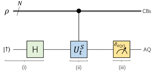
Figure 1: Scheme for probing the characteristic function of statistical quantity X by a quantum simulator. (i) Initial state preparations. The classical spin (bit) systems (CBs) and the auxiliary qubit (AQ) are prepared respectively in probability distribution $\rho$ (or a thermal equilibrium state $\rho_{\mathrm{th}}$ discussed in the main text), and a superposition state $\left|+\right\rangle=(\left|\downarrow\right\rangle+\left|\uparrow\right\rangle)/\sqrt{2}$ by a Hadamard gate. (ii) The information of the characteristic function is encoded into the auxiliary qubit by a simulated unitary operator $U_{t}^{S}$ (see e.g., Fig. 2(a) and Fig. 3(a) respectively for the detection of magnetization order parameter and kink number). (iii) The real and imaginary parts of the characteristic function are detected by $\left\langle\hat{\sigma}_{x}\right\rangle$ and $\left\langle\hat{\sigma}_{y}\right\rangle$ respectively.

Probing the characteristic function with an auxiliary qubit.— A schematic diagram for the detection of characteristic functions with an auxiliary qubit is shown in Fig. 1. The proposed experimental protocol consists of the following steps:

Step 1: The probe qubit is first prepared in the quantum superposition state $\left|+\right\rangle=(\left|\downarrow\right\rangle+\left|\uparrow\right\rangle)/\sqrt{2}$ by the action of a Hadamard gate $\mathrm{H}=(\hat{\sigma}_{x}+\hat{\sigma}_{z})/\sqrt{2}$ ($\hat{\sigma}_{x,y,z}$ stand for Pauli matrices). The classical spin system is prepared in the canonical thermal equilibrium state $\rho_{\mathrm{th}}$.

Step 2: The evolution of the composite system is simulated by $U_{t}^{S}=\exp(-iH_{\mathrm{int}}t)$ with $H_{\mathrm{int}}=\epsilon\hat{\sigma}_{z}X$ ($\epsilon$ denotes a coupling constant), which can be further written in an explicit form as

$$U_{t}^{S}=e^{-ita\epsilon\hat{\sigma}_{z}}\prod_{\{n_{1},\cdots,n_{l}\}}^{N}\exp\left(-itb\epsilon\hat{\sigma}_{z}\sigma_{n_{1}}\cdots\sigma_{n_{l}}\right).$$ (9)

This unitary operator can be implemented via digital quantum simulation Lloyd (1996). Then, the time-evolved state reads

$$\rho_{t}=\frac{1}{2}(e^{i\Omega t}\left|\downarrow\right\rangle+\left|\uparrow\right\rangle)(e^{-i\Omega t}\left\langle\downarrow\right|+\left\langle\uparrow\right|)\rho_{\mathrm{th}},$$ (10)

where $\Omega=2\epsilon X$.

Step 3: The coherence of the probe spin measured by monitoring the operator $2\hat{\sigma}_{+}=\hat{\sigma}_{x}+i\hat{\sigma}_{y}$, i.e.,

$$\left\langle\hat{\sigma}_{x}\right\rangle+i\left\langle\hat{\sigma}_{y}\right\rangle=\sum_{\{\sigma_{n}=\pm 1\}}e^{i\mathrm{\Omega}t}\rho_{\mathrm{th}}=e^{i2\epsilon at}\frac{Z(\mathcal{\tilde{J}}^{\prime},\tilde{h}^{\prime},\beta)}{Z(\mathcal{J},h,\beta)},$$ (11)

where $Z(\mathcal{\tilde{J}}^{\prime},\tilde{h}^{\prime},\beta)=\sum_{\{\sigma=\pm 1\}}e^{-\beta H_{\mathrm{s}}(\mathcal{J},h)}e^{i2\epsilon t(X-a)}$. Parameters $\mathcal{\tilde{J}}^{\prime}$ and $\tilde{h}^{\prime}$ represent the effectively complex spin coupling constants and the complex magnetic field, respectively, which are dependent on the specific choice of $X$. If we select $2\epsilon t=\theta$, we have $\mathcal{\tilde{J}}^{\prime}=\mathcal{\tilde{J}}$ and $\tilde{h}^{\prime}=\tilde{h}$. Then Eq. (S19) is exactly the same as the characteristic function in Eq. (8). After performing the Fourier transformation, the full distribution of $X$ can be immediately reconstructed.

In what follows we illustrate the above general scheme by analyzing two instances of $X$: the magnetization $M$ and kink number $K$ for a finite-temperature Ising chain.

Example 1: Measuring the full distribution of the magnetization.— Let us consider the Ising chain with nearest-neighbor interactions described by the Hamiltonian

$$H_{\mathrm{s}}(J,h)=-J\sum_{n=1}^{N}\sigma_{n}\sigma_{n+1}-h\sum_{n=1}^{N}\sigma_{n},$$ (12)

with the periodic boundary condition $\sigma_{N+1}=\sigma_{1}$. The analytically-continued partition function can be derived by the method of transfer matrix Plischke and Bergersen (2006), which yields

$$Z(J,h,\beta)=\lambda_{-}^{N}+\lambda_{+}^{N},$$ (13)

where $\lambda_{\pm}=e^{\beta J}\cosh(\beta h)\pm e^{-\beta J}\sqrt{1+e^{4\beta J}\sinh^{2}(\beta h)}$. The magnetization, Eq. (2), is the order parameter. To determine its full distribution, we note that the numerator of the characteristic function Eq. (8) can be written as $Z(J,\tilde{h},\beta)$, where $\tilde{h}=h+i\theta/\beta$ is the complex magnetic field.

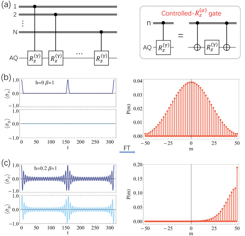
Figure 2: Probing the distribution of the magnetization in a nearest-neighbor Ising chain. (a) A schematic quantum circuit for simulating the evolution of the composite system $U_{t}^{S}=\prod_{n=1}^{N}\exp\left(-it\epsilon\hat{\sigma}_{z}\sigma_{n}\right)$ [Eq. (14)]. The kernel of $U_{t}^{S}$ is realized by a controlled-$R_{z}^{(\gamma)}$ gate ($\gamma=2\epsilon t$), with $R_{z}^{(\alpha)}=\exp(-\frac{i\alpha}{2}\hat{\sigma}_{z})$. Note that for the controlled-NOT gate, the target qubit is flipped if the control classical bit is set to $\sigma_{n}=-1$. The characteristic function of the magnetization distribution is detected by the coherence function of an auxiliary qubit. For an Ising chain of $N=50$ spins at inverse temperature $\beta=1$ with magnetic field (b) $h=0$ and (c) $h=0.2$, the real ($\left\langle\hat{\sigma}_{x}\right\rangle$) and imaginary ($\left\langle\hat{\sigma}_{y}\right\rangle$) parts of the coherence function are displayed as a function of time $t\in[0,\pi/\epsilon]$, with the spin-qubit coupling $\epsilon=0.01$. The right panels of (b) and (c) correspond to the probability distribution of the magnetization obtained by Fourier transform (FT) of the characteristic function.

To measure the characteristic function, we use the general scheme introduced above with the unitary

$$U_{t}^{S}=\prod_{n=1}^{N}\exp\left(-it\epsilon\hat{\sigma}_{z}\sigma_{n}\right),$$ (14)

which can be simulated with quantum logical circuit depicted in Fig. 2(a). After measuring the real and imaginary parts of the coherence function of the auxiliary qubit, and performing the Fourier transformation, the distribution $P(m)$ is obtained. See examples with $h=0$ and $h=0.2$ in Fig. 2(b) and (c), respectively. Note that the magnetization varies in jumps of two units. For an even number of spins $N$, $P(m)=0$ for odd $m$, while for odd $N$, $P(m)=0$ for even $m$. We notice that our approach can be readily applied to long-range spin systems as shown in the Supplemental Material SM .

The cumulant generating function of the magnetization, which is the logarithm of the characteristic function, admits the following expansion

$$\log F(\theta)=\sum_{j=1}^{\infty}\kappa_{j}\frac{(i\theta)^{j}}{j!}.$$ (15)

In the large $N$ limit, one can invoke the approximation $Z(J,\widetilde{h},\beta)\approx\lambda_{+}^{N}(\theta)$. Explicit computation yields the following expressions for the first few cumulants (related to the mean, variance, and skewness)

$$\kappa_{1} = \langle M\rangle=Nu^{-1}e^{2\beta J}\sinh(\beta h),$$ (16)

$$\kappa_{2} = \mathrm{Var}(M)=Nu^{-3}e^{2\beta J}\cosh(\beta h),$$ (17)

$$\kappa_{3} = \mathrm{Skew}(M)\kappa_{2}^{3/2}=Nu^{-5}ve^{2\beta J}\sinh(\beta h),$$ (18)

the first two being well known (see e.g. Plischke and Bergersen (2006)), where $u=\sqrt{1+e^{4\beta J}\sinh^{2}(\beta h)}$ and $v=1-e^{4\beta J}[2+\cosh(2\beta h)]$ for short. The finiteness of $\kappa_{q}$ with $q>2$ makes $P(m)$ manifestly non-normal. In the large $N$ limit, all cumulants of $P(m)$ scale linearly with the system size $N$. As a result, the ratio between the amplitude of the fluctuations quantified by the root mean square $\Delta M=\kappa_{2}^{1/2}$ and the average magnetization per spin $\langle M\rangle$ is proportional to $\Delta M/\langle M\rangle\propto N^{-1/2}$ and fluctuations are suppressed in the thermodynamic limit. Keeping $\kappa_{1}$ and $\kappa_{2}$ and ignoring higher-order cumulants, the probability distribution can then be approximated by a Gaussian $P(m)=C\exp[-(m-\langle M\rangle)^{2}/(2\mathrm{Var}(M))]$, with support on $M\in[-N,N]$, with $C$ a normalization constant. Deviations from this limit are manifested for nonzero values of $h$.

Example 2: Measuring the full kink-number distribution.— In spin systems, kinks are localized at the interface between adjacent domains. We next consider the distribution of the number of kinks. Considering Eq. (3), the corresponding complex parameters in the analytically-continued partition function in the numerator of Eq. (8) are given by $\tilde{J}=J-\frac{i\theta}{2\beta}$, and $\tilde{h}=h$.

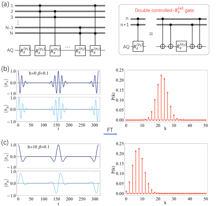
Figure 3: Probing the distribution of the kink number in a nearest-neighbor Ising chain. (a) A schematic quantum circuit for simulating the evolution of the composite system $U_{t}^{S}=e^{-it\frac{N}{2}\epsilon\hat{\sigma}_{z}}\prod_{n=1}^{N}\exp\left(it\frac{\epsilon}{2}\hat{\sigma}_{z}\sigma_{n}\sigma_{n+1}\right)$ [Eq. (19)], with $\gamma_{1}=N\epsilon t$ and $\gamma_{2}=-\epsilon t$. The real ($\left\langle\hat{\sigma}_{x}\right\rangle$) and imaginary ($\left\langle\hat{\sigma}_{y}\right\rangle$) parts of the coherence function are displayed as a function of time $t\in[0,\pi/\epsilon]$, with the spin-qubit coupling $\epsilon=0.01$, $N=50$, $\beta=0.1$ and magnetic field $h=0$ in (b) and $h=10$ in (c). The right parts of (b) and (c) are the probability distribution of the kink number.

The general scheme can be used to experimentally determine the characteristic function, choosing

$$U_{t}^{S}=e^{-it\frac{N}{2}\epsilon\hat{\sigma}_{z}}\prod_{n=1}^{N}\exp\left(it\frac{\epsilon}{2}\hat{\sigma}_{z}\sigma_{n}\sigma_{n+1}\right),$$ (19)

which can be simulated with quantum logical circuit shown in Fig. 3(a). For different values of $h$ and $\beta$, monitoring the coherence of the qubit allows one to reconstruct the full kink-number distribution $P(k)$.

The logarithm of the characteristic function of the kink-number distribution is the corresponding cumulant generating function. For the nearest-neighbor Ising model, approximating the partition function in the large $N$ limit by the largest eigenvalue $Z(\tilde{J},h,\beta)\approx\lambda_{+}^{N}(\theta)$, one finds the first cumulant, that equals the mean number of kinks

$$\left\langle K\right\rangle=\frac{N}{u\lambda_{+}e^{\beta J}}.$$ (20)

At zero field, $h=0$, this expression reduces to $\langle K\rangle=N/(1+e^{2\beta J})$, which varies from $0$ to $N/2$ as the temperature is increased. The explicit expression for the variance is given by

$$\mathrm{Var}(K)=\frac{N\left[\cosh(\beta h)+2e^{3\beta J}\sinh^{2}(\beta h)\lambda_{+}\right]}{u^{3}\lambda_{+}^{2}},$$ (21)

which reduces to $Ne^{2\beta J}(1+e^{2\beta J})^{-2}$ when $h=0$. While higher cumulants can be found making use of the expansion (15) with the corresponding characteristic function, their expression becomes increasingly cumbersome (see e.g. the third cumulant $\kappa_{3}$ in SM ). At zero magnetic field, the standard deviation $\Delta K=\sqrt{\mathrm{Var}(K)}$ over the mean vanishes as one approaches the thermodynamic limit with increasing system size $N$ as

$$\frac{\Delta K}{\langle K\rangle}=\frac{e^{\beta J}}{\sqrt{N}},$$ (22)

and $P(k)$ approaches the normal distribution.

Non-normal features of $P(k)$ arising from non-vanishing cumulants $\kappa_{q}$ with $q>2$ become apparent at finite values of the magnetic field, see Figs. 3(b)-(c), as well as low temperatures.

Discussions.— The scheme for probing the full distributions of magnetization and kink number in quantum systems is similar to the classical case. Assume the auxiliary qubit and the quantum spin system are initially prepared in state $\left|+\right\rangle\left\langle+\right|\otimes\rho$, where $\rho$ is an arbitrary quantum state of the system, e.g., in or out of equilibrium. A Hadamard gate is applied to the auxiliary qubit after performing a controlled gate $U_{\theta}^{S}=\left|\uparrow\right\rangle\left\langle\uparrow\right|\otimes\exp(i\theta X)+\left|\downarrow\right\rangle\left\langle\downarrow\right|\otimes\mathbb{I}$ on the whole system. The state of the auxiliary qubit is then given by tr${}_{spins}[(\mathrm{H}\otimes\mathbb{I)}U_{\theta}^{S}(\left|+\right\rangle\left\langle+\right|\otimes\rho)U_{\theta}^{S{\dagger}}(\mathrm{H}\otimes\mathbb{I)}]=[\mathbb{I+}\hat{\sigma}_{z}\text{Re}F(\theta)+\hat{\sigma}_{y}\text{Im}F(\theta)]/2$. Thus, the real and imaginary parts of the characteristic function $F(\theta)$ can be recovered by measuring the operators $\hat{\sigma}_{z}$ and $\hat{\sigma}_{y}$, respectively, on the auxiliary qubit. See SM for an alternative scheme. While the experimental protocol can thus be adapted for quantum systems SM , the equilibrium relation between $F(\theta)$ and the analytically-continued partition function is generally lost as the system Hamiltonian $H_{s}$ and $X$ do not necessarily commute. Similarly, for nonequilibrium states, whether quantum or classical, the measurement protocol applies but the connection with the partition function is lost.

Summary.— We have presented a general scheme to experimentally measure the full distribution of the many-body observables in classical and quantum systems, using an auxiliary qubit as a probe. We have demonstrated our scheme by considering the distribution of the magnetization and the number of kinks in classical spin systems. In this setting, the characteristic functions of the corresponding equilibrium distributions have been shown to be directly given by the analytic continuation of the partition function. This connection is readily applicable to other spin systems where the partition function in the presence of a magnetic field is at reach, such as Heisenberg spin chains Fisher (1964); Cregg et al. (2008). We note that the analytic continuation of the partition function has already been measured experimentally in the determination of Lee-Yang zeroes in a NMR setting Peng et al. (2015). Our proposal is within reach of current technology. While we have focused on the determination of the magnetization and kink-number distributions at equilibrium, we emphasize that our scheme can be also applied to scenarios away from equilibrium. Our findings should therefore find broad applications in the characterization of many-body spin systems across different disciplines, including statistical mechanics, condensed matter or magnetometry.

Acknowledgment.- It is a pleasure to acknowledge discussions with Fernando Javier Gómez-Ruiz, Luis Pedro García-Pintos, Kohei Kawabata, Geza Toth and Masahito Ueda. Funding support from the John Templeton Foundation, UMass Boston (project P20150000029279), and the National Natural Science Foundation of China (Grant No. 11674238) is further acknowledged.

Supplemental Material

I I. Higher cumulants for the distribution of kink number in the Ising chain

As noted in the main text, the characteristic function $F(\theta)$ of the kink distribution $P(k)$ is given by the analytic continuation of the partition function

$$F(\theta)=Z(\tilde{J},h,\beta)=\lambda_{-}^{N}+\lambda_{+}^{N},$$ (S1)

with $\tilde{J}=J-\frac{i\theta}{2\beta}$. Using a cumulant expansion, one can readily find an arbitrary cumulant. The exact first cumulant ($h=0$) reads

$$\langle K\rangle=\frac{N}{2}e^{-\beta J}\frac{\cosh^{N-1}(\beta J)-\sinh^{N-1}(\beta J)}{\cosh^{N}(\beta J)+\sinh^{N}(\beta J)}.$$ (S2)

The exact expressions of higher order cumulants are somewhat cumbersome. Using the simplified expression for the partition function $Z(\tilde{J},h,\beta)\approx\lambda_{+}^{N}(\theta)$, the cumulants admit simpler expressions (see e.g. $\kappa_{1}$ and $\kappa_{2}$ in the main text). In particular, the third cumulant, which is proportional to the skewness, reads

$$\kappa_{3}=\mathrm{Skew}(K)\kappa_{2}^{3/2}=\frac{Ne^{-\beta J}\left[5e^{2\beta J}-(2+w)e^{2\beta J}\cosh(2\beta h)-2uw\cosh(\beta h)+4(u^{2}-1)\lambda_{-}e^{\beta J}\cosh(\beta h)\right]}{2u^{5}\lambda_{+}^{3}},$$ (S3)

where $w=1-8e^{8\beta J}\sinh^{4}(\beta h)$.

One readily finds that the cumulant generating function is proportional to the system size, as $\log F(\theta)\approx N\log\lambda_{+}^{N}(\theta)$, where $\lambda_{+}^{N}(\theta)$ is independent of $N$. Thus, all cumulants of the distribution scale linearly with $N$.

II II. Probing magnetization order parameter and kink number in long-range Ising chain

The quantum circuit for the simulation of $U_{t}^{S}$ is only dependent on the statistical quantity we are going to measure, but independent of the specific spin system under study, i.e., it is not specific of the short-range Ising chain. As such, it can be applied to the characterization of the distribution of many-body observables in other experimentally relevant spin systems. Let us consider the long-range Ising model, with the following Hamiltonian

$$H_{\mathrm{s}}\left(J,h\right)=-J\sum_{m<n}^{N}\sigma_{m}\sigma_{n}-h\sum_{n=1}^{N}\sigma_{n},$$ (S4)

involving all-to-all pairwise interactions of equal strength. This model arises naturally in an NMR setting Peng et al. (2015). The corresponding partition function is given by

$$Z(J,h,\beta)=e^{\frac{N(N-1)\beta J}{2}}e^{N\beta h}\sum_{n=0}^{N}\binom{N}{n}e^{-2\beta hn}e^{2\beta J(n^{2}-Nn)}.$$ (S5)

In what follows we discuss the experimental protocol to characterize both the magnetization and kink-number distributions in this system.

II.1 A. Probing the probabilistic distribution of magnetization order parameter

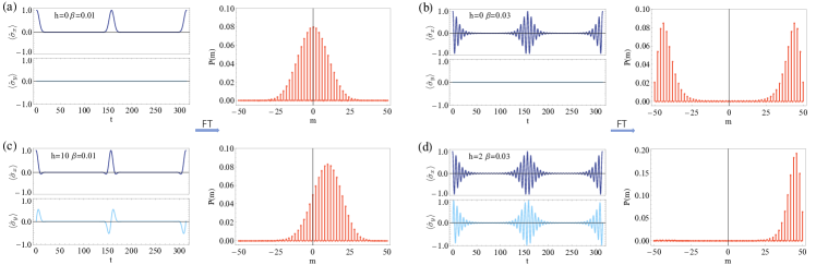
Figure SM1: Distribution of the magnetization in a long-range Ising model. The real ($\left\langle\hat{\sigma}_{x}\right\rangle$) and imaginary ($\left\langle\hat{\sigma}_{y}\right\rangle$) parts of the coherence function of the auxiliary qubit are detected as a function of time $t\in[0,\pi/\epsilon]$, with spin number $N=50$, the spin-qubit coupling $\epsilon=0.01$, and inverse temperature $\beta=0.01$ when the magnetic field (a) $h=0$ and (c) $h=10$; $\beta=0.03$ when the magnetic field (b) $h=0$ and (d) $h=2$. The probability distribution function $P(m)$ is constructed by performing the Fourier transformation.

The characteristic function of the magnetization distribution $P(m)$ can be written as

$$F(\theta)=\frac{Z(J,h+\frac{i\theta}{\beta},\beta)}{Z(J,h,\beta)},$$ (S6)

which admits the explicit form

$$F(\theta)=\frac{e^{iN\theta}\sum_{n=0}^{N}e^{-2in\theta}g(n)}{\sum_{n=0}^{N}g(n)},$$ (S7)

where $g(n)=\binom{N}{n}e^{-2\beta hn}e^{2\beta J(n^{2}-Nn)}$. Use of the cumulant expansion readily yields the first few cumulants of $P(m)$

$$\kappa_{1}=\left\langle M\right\rangle = N-\frac{2G_{1}(N)}{G_{0}(N)},$$ (S8)

$$\kappa_{2}=\mathrm{Var}(M) = 4\left[\frac{G_{2}(N)}{G_{0}(N)}-\left(\frac{G_{1}(N)}{G_{0}(N)}\right)^{2}\right],$$ (S9)

$$\kappa_{3}=\mathrm{Skew}(M)\kappa_{2}^{3/2} = -8\left[\frac{G_{3}(N)}{G_{0}(N)}-3\frac{G_{1}(N)G_{2}(N)}{G_{0}(N)^{2}}+2\left(\frac{G_{1}(N)}{G_{0}(N)}\right)^{3}\right],$$ (S10)

where $G_{\alpha}(N)=\sum_{n=1}^{N}n^{\alpha}g(n)$.

The experimental proposal for probing the characteristic function is similar to Example 1 in the main text, with numerical simulations shown in Fig. (SM1).

II.2 B. Probing the probabilistic distribution of kink number

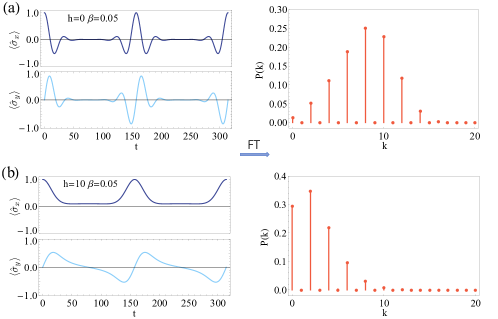
Figure SM2: Distribution of the kink number in a long-range Ising model. The real ($\left\langle\hat{\sigma}_{x}\right\rangle$) and imaginary ($\left\langle\hat{\sigma}_{y}\right\rangle$) parts of the coherence function of the auxiliary qubit are displayed as a function of time $t\in[0,\pi/\epsilon]$, with spin number $N=20$, the spin-qubit coupling $\epsilon=0.01$, inverse temperature $\beta=0.05$, and the magnetic field (a) $h=0$ and (b) $h=10$. The probability distribution function $P(k)$ is shown after Fourier transformation.

The characteristic function is given by

$$F(\theta)=e^{i\frac{N\theta}{2}}\frac{Z(\mathcal{\tilde{J}},h,\beta)}{Z(J,h,\beta)},$$ (S11)

where

$$\mathcal{\tilde{J}}=\left\{\begin{array}[]{ll}J&n\neq m+1\\ J-\frac{i\theta}{2\beta}&n=m+1\end{array}\right.$$ (S12)

The experimental proposal for probing the characteristic function is similar to Example 2 in the main text, with numerical simulations shown in Fig. (SM2).

III III. Probing the characteristic function for quantum spin systems

III.1 A. Quantum circuit

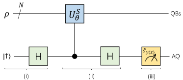
Figure SM3: Scheme for probing the characteristic function of quantum spin systems by a quantum simulator. (i) Initial state preparations. The quantum spin (qubit) systems (QBs) and the auxiliary qubit (AQ) are prepared respectively in state $\rho$, and a superposition state $\left|+\right\rangle=(\left|\downarrow\right\rangle+\left|\uparrow\right\rangle)/\sqrt{2}$ by a Hadamard gate. (ii) The information of the characteristic function is encoded into the auxiliary qubit by a simulated unitary operator $U_{\theta}^{s}$ and a Hadamard gate. (iii) The real and imaginary parts of the characteristic function are detected by $\left\langle\hat{\sigma}_{z}\right\rangle$ and $\left\langle\hat{\sigma}_{y}\right\rangle$ respectively.

The scheme for probing the characteristic function for quantum spin systems is shown in Fig. (SM3), which is slightly different from the classical case in the main text.

III.2 B. Probing the magnetization distribution via Loschmidt echo

We have seen that the characteristic function of the magnetization is related to the analytic continuation of the partition function. In quantum systems, the later can be measured in a variety of quantum platforms including quantum simulators of spin systems and NMR experiments. Given a Hamiltonian $H$ with eigenvalues $E_{n}$ and energy eigenstates $|n\rangle$, the state of the system can be initialized in the coherent quantum superposition of the form $|\psi(0)\rangle=\sum_{n}\sqrt{p_{n}}|n\rangle$ where $p_{n}=\exp(-\beta E_{n})/Z(\beta)$ and $Z(\beta)=\sum_{n}\exp(-\beta E_{n})$ denotes the partition function. This superposition evolves into $|\psi(t)\rangle=\sum_{n}\exp[-(\beta/2+it)E_{n}]|n\rangle/\sqrt{Z(\beta)}$, and the survival amplitude reads $\langle\psi(0)|\psi(t)\rangle=Z(\beta+it)/Z(\beta)$. Choosing as a Hamiltonian the Ising chain, the survival amplitude can be written as $\langle\psi(0)|\psi(t)\rangle=Z(\beta,h-it/\beta)/Z(\beta,h)$, this is, in terms of the analytically continued partition function for an Ising chain with a complex-valued magnetic field, and can be measured experimentally via a Loschmidt echo Peng et al. (2015). Its Fourier transform directly yields the full distribution of the magnetization.

IV IV. Simulation efficiency and error analysis

In this section, we provide a brief analysis on the simulation efficiency and possible experimental errors.

IV.1 A. An estimation of simulation efficiency

In the main text, the evolution of the composite system is given by $U_{t}^{S}=\exp(-iH_{\mathrm{int}}t)$ with

$$H_{\mathrm{int}}=\epsilon\hat{\sigma}_{z}X=\epsilon a\hat{\sigma}_{z}+\epsilon b\hat{\sigma}_{z}\sum_{\{n_{1},\cdots,n_{l}\}}^{N}H_{\{n_{1},\cdots,n_{l}\}},$$ (S13)

where $\epsilon$ denotes a coupling constant, and $H_{\{n_{1},\cdots,n_{l}\}}=\sigma_{n_{1}}\cdots\sigma_{n_{l}}$ is a many-body spin interaction. Since the spin system is classical, all $H_{\{n_{1},\cdots,n_{l}\}}$ commute and $U_{t}^{S}$ can be directly decomposed as

$$U_{t}^{S}=e^{-iH_{\mathrm{int}}t}=e^{-ita\epsilon\hat{\sigma}_{z}}\prod_{\{n_{1},\cdots,n_{l}\}}^{N}\exp(-itb\epsilon\hat{\sigma}_{z}H_{\{n_{1},\cdots,n_{l}\}}),$$ (S14)

with no approximation, and each $e^{-itb\epsilon\hat{\sigma}_{z}H_{\{n_{1},\cdots,n_{l}\}}}$ can be realized by digital simulations with logical gates (as shown in the main text). Note that although there is no simulation error in this case, operational errors in the lab cannot be avoided (see an analysis of possible experimental errors in Sec. IV.2).

In the discussion in the main text, we also consider quantum spin systems. The distribution of many-body observables

$$X=a+b\sum_{\{n_{1},\cdots,n_{l}\}}^{N}H_{\{n_{1},\cdots,n_{l}\}},\text{ with }H_{\{n_{1},\cdots,n_{l}\}}=\hat{\sigma}_{\alpha_{1};n_{1}}\cdots\hat{\sigma}_{\alpha_{l};n_{l}},\text{ (}\alpha_{n_{j}}=x,y,z\text{),}$$ (S15)

can still be detected by coupling to a single probe qubit and monitoring its coherence. The scheme requires to simulate $U_{\theta}^{S}=\left|\uparrow\right\rangle\left\langle\uparrow\right|\otimes e^{i\theta X}+\left|\downarrow\right\rangle\left\langle\downarrow\right|\otimes\mathbb{I}$, in which the operator $e^{i\theta X}$ can be further written in an explicit form as

$$e^{i\theta X}=e^{e^{i\theta a}}e^{i\theta b\sum_{\{n_{1},\cdots,n_{l}\}}^{N}H_{\{n_{1},\cdots,n_{l}\}}}.$$ (S16)

We note that, if we only consider the magnetization $M=\sum_{n=1}^{N}\hat{\sigma}_{z;n}$ and the kink number $K=\frac{1}{2}(N-\sum_{n=1}^{N}\hat{\sigma}_{z;n}\hat{\sigma}_{z;n+1})$, there will also be no simulation error since the items in the sum of Eq. (S16) all commute. However, for general many-body observables, each $H_{\{n_{1},\cdots,n_{l}\}}$ may not commute. To realize such scheme in digital quantum simulations, we have to perform some approximations. One method is to employ Suzuki-Trotter expansion with $m$ steps. For any $\varepsilon>0$, $m$ can always be chosen sufficiently large to ensure that $e^{i\theta X}$ is well approximated by the simulator with an error no greater than $\varepsilon$, i.e.,

$$\left\|e^{i\theta X}-e^{e^{i\theta a}}\left(\prod_{\{n_{1},\cdots,n_{l}\}}^{N}e^{\frac{i\theta bH_{\{n_{1},\cdots,n_{l}\}}}{m}}\right)^{m}\right\|\leq\varepsilon.$$ (S17)

This “digital” approach to quantum simulation [Eq. (S17)] aimed at probing the statistics of general many-body observables is efficient since the number of the combination in $\{n_{1},\cdots,n_{l}\}$ is around $N^{n_{l}}/n_{l}!$ ($n_{l}\ll N$), which is a polynomial function of $N$ Lloyd (1996).

IV.2 B. Experimental error analysis

The analysis above shows that if the spin chain systems are classical (or quantum spin chains with observables such as the magnetization and the kink number), there will be no simulation errors (i.e., $U_{\mathrm{simulation}}\equiv U_{\mathrm{exact}}$). However the operational errors in experiment can not be neglected, and may influence the accuracy of the final full distribution with an error propagation

$$\text{Experimental errors}\rightarrow\text{Characteristic Function }F\text{(}\theta\text{)}\rightarrow\text{Distribution }P.$$ (S18)

The main experimental errors we consider here stem from the imperfect implementation of logical gates and the decoherence of the auxiliary qubit.

In NMR systems, the universal logical gates (i.e., single qubit rotation and CNOT gates) can currently be realized by the gradient ascent pulse engineering (GRAPE) technique with very high precision (pulses fidelity around 99.95%) Lu et al. (2016). The imperfection errors can be neglected within such a high accuracy. For the auxiliary qubit, the $T_{2}^{\ast}$ can be of the order of several seconds. A CNOT gate and single qubit rotation gate can be implemented within several milliseconds Lu et al. (2016). Therefore, it is possible to implement hundreds of gates before $T_{2}^{\ast}$ has elapsed. For example, if we adopt the trimethyl phosphite system (consisting of $9$ ¹H spins as the spin chain and one ³¹P nuclear spin as the auxiliary probe qubit) in the Lee-Yang zeros experiment Peng et al. (2015), the total number of universal gates is $27$ [$=$($1$ single qubit rotation gate$+2$ CNOT gates)$\times 9$] for the magnetization. These gates can be finished within around 300 milliseconds, which is much less than the $T_{2}^{\ast}$ of the auxiliary qubit. Therefore, our scheme is available with current NMR experimental techniques.

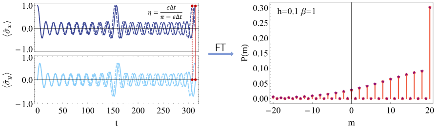
Figure SM4: Error analysis for imperfect implementation of logical gates. Example: Probing the distribution of the magnetization order parameter in a nearest-neighbor Ising chain ($N=20$, $h=0.1$, $\beta=1$, and $\epsilon=0.01$). Left: the real ($\left\langle\hat{\sigma}_{x}\right\rangle$) and imaginary ($\left\langle\hat{\sigma}_{y}\right\rangle$) parts of the characteristic function are displayed as a function of time $t\in[0,\pi/\epsilon]$ with no operational errors of logical gates (solid curves) and with errors $\eta$ (dashed curves). The error $\eta$ can be evaluated by measuring the $\Delta t$ (the time interval between the solid and dashed red lines). Right: The probability distribution of the magnetization obtained by Fourier transform (FT) of the characteristic function with no errors (red dots) and by the modified FT [Eq. (S20)] with errors (purple stars). Obviously, such kind of operational errors can be circumvented in experiment.

Note that even when the gate errors can not be neglected, there is a method to circumvent such errors. Every kernel $\exp\left(-itb\epsilon\hat{\sigma}_{z}\sigma_{n_{1}}\cdots\sigma_{n_{l}}\right)$ in Eq. (S14) can be realized by a controlled rotation gate (as shown in the main text). We assume the error of such gate is $\delta=\eta\epsilon$, then $\epsilon^{\prime}=\epsilon+\delta=(1+\eta)\epsilon$. Following the operation steps in the main text, the coherence of the probe spin is then given by

$$\left\langle\hat{\sigma}_{x}\right\rangle+i\left\langle\hat{\sigma}_{y}\right\rangle=e^{i2\epsilon at}\frac{Z(\mathcal{\tilde{J}}^{\prime},\tilde{h}^{\prime},\beta,\epsilon^{\prime})}{Z(\mathcal{J},h,\beta,\epsilon)},$$ (S19)

where $Z(\mathcal{\tilde{J}}^{\prime},\tilde{h}^{\prime},\beta,\epsilon^{\prime})=\sum_{\{\sigma=\pm 1\}}e^{-\beta H_{\mathrm{s}}(\mathcal{J},h)}e^{i2\epsilon^{\prime}t(X-a)}$. If we set $2\epsilon t=\theta$, Eq. (S19) is the final characteristic function (including the errors of logical gates). In real experiment, we may directly perform the frequency domain measurements to get the full distribution or adopt the indirect measurement. For the latter, the distribution of X (with errors) can be reconstructed by performing the Fourier transformation. However, if we know the error of such logical gate, there is one method to circumvent such errors with the following revised Fourier transform

$$P(x)=\frac{1+\eta}{2\pi}\int_{0}^{\frac{2\pi}{1+\eta}}d\theta F[\theta(1+\eta)]e^{-ix\theta(1+\eta)},$$ (S20)

with which we can reconstruct the $P(x)$. In Fig. (SM4), we illustrate such scheme with the example of measuring the distribution of magnetization ($\eta=0.02$ as an example).

References

- Binder (1981) K. Binder, Zeitschrift für Physik B Condensed Matter 43, 119 (1981).
- Bruce (1981) A. D. Bruce, Journal of Physics C: Solid State Physics 14, 3667 (1981).
- Bruce (1985) A. D. Bruce, Journal of Physics A: Mathematical and General 18, L873 (1985).
- Nicolaides and Bruce (1988) D. Nicolaides and A. D. Bruce, Journal of Physics A: Mathematical and General 21, 233 (1988).
- Bruce and Wilding (1992) A. D. Bruce and N. B. Wilding, Phys. Rev. Lett. 68, 193 (1992).
- Bramwell et al. (1998) S. T. Bramwell, P. C. W. Holdsworth, and J.-F. Pinton, Nature 396, 552 (1998).
- Aji and Goldenfeld (2001) V. Aji and N. Goldenfeld, Phys. Rev. Lett. 86, 1007 (2001).
- Shinjo (2013) T. Shinjo, Nanomagnetism and Spintronics-Second Editon (Elsevier, 2013).
- Denisov and Hänggi (2005) S. I. Denisov and P. Hänggi, Phys. Rev. E 71, 046137 (2005).
- del Campo and Zurek (2014) A. del Campo and W. H. Zurek, International Journal of Modern Physics A 29, 1430018 (2014).
- del Campo (2018) A. del Campo, Phys. Rev. Lett. 121, 200601 (2018).
- Fedichev and Fischer (2003) P. O. Fedichev and U. R. Fischer, Phys. Rev. Lett. 91, 240407 (2003).
- Recati et al. (2005) A. Recati, P. O. Fedichev, W. Zwerger, J. von Delft, and P. Zoller, Phys. Rev. Lett. 94, 040404 (2005).
- Hangleiter et al. (2015) D. Hangleiter, M. T. Mitchison, T. H. Johnson, M. Bruderer, M. B. Plenio, and D. Jaksch, Phys. Rev. A 91, 013611 (2015).
- Elliott and Johnson (2016) T. J. Elliott and T. H. Johnson, Phys. Rev. A 93, 043612 (2016).
- Quan et al. (2006) H. T. Quan, Z. Song, X. F. Liu, P. Zanardi, and C. P. Sun, Phys. Rev. Lett. 96, 140604 (2006).
- Zhang et al. (2008) J. Zhang, X. Peng, N. Rajendran, and D. Suter, Phys. Rev. Lett. 100, 100501 (2008).
- Goold et al. (2011) J. Goold, T. Fogarty, N. Lo Gullo, M. Paternostro, and T. Busch, Phys. Rev. A 84, 063632 (2011).
- Knap et al. (2012) M. Knap, A. Shashi, Y. Nishida, A. Imambekov, D. A. Abanin, and E. Demler, Phys. Rev. X 2, 041020 (2012).
- Damski et al. (2011) B. Damski, H. T. Quan, and W. H. Zurek, Phys. Rev. A 83, 062104 (2011).
- Dorner et al. (2013) R. Dorner, S. R. Clark, L. Heaney, R. Fazio, J. Goold, and V. Vedral, Phys. Rev. Lett. 110, 230601 (2013).
- Mazzola et al. (2013) L. Mazzola, G. De Chiara, and M. Paternostro, Phys. Rev. Lett. 110, 230602 (2013).
- Roncaglia et al. (2014) A. J. Roncaglia, F. Cerisola, and J. P. Paz, Phys. Rev. Lett. 113, 250601 (2014).
- Batalhão et al. (2014) T. B. Batalhão, A. M. Souza, L. Mazzola, R. Auccaise, R. S. Sarthour, I. S. Oliveira, J. Goold, G. De Chiara, M. Paternostro, and R. M. Serra, Phys. Rev. Lett. 113, 140601 (2014).
- Correa et al. (2015) L. A. Correa, M. Mehboudi, G. Adesso, and A. Sanpera, Phys. Rev. Lett. 114, 220405 (2015).
- Swingle et al. (2016) B. Swingle, G. Bentsen, M. Schleier-Smith, and P. Hayden, Phys. Rev. A 94, 040302 (2016).
- García-Álvarez et al. (2017) L. García-Álvarez, I. L. Egusquiza, L. Lamata, A. del Campo, J. Sonner, and E. Solano, Phys. Rev. Lett. 119, 040501 (2017).
- Wei and Liu (2012) B.-B. Wei and R.-B. Liu, Phys. Rev. Lett. 109, 185701 (2012).
- Wei et al. (2014) B.-B. Wei, S.-W. Chen, H.-C. Po, and R.-B. Liu, Sci. Rep. 4, 5202 (2014).
- Peng et al. (2015) X. Peng, H. Zhou, B.-B. Wei, J. Cui, J. Du, and R.-B. Liu, Phys. Rev. Lett. 114, 010601 (2015).
- Lu et al. (2016) D. Lu, A. Brodutch, J. Park, H. Katiyar, T. Jochym-O’Connor, and R. Laflamme, NMR Quantum Information Processing, edited by T. Takui, L. Berliner, and G. Hanson (Springer, New York, 2016) pp. 193–226.
- Goldenfeld (1992) N. Goldenfeld, Lectures On Phase Transitions And The Renormalization Group (Addison-Wesley, 1992).
- Plischke and Bergersen (2006) M. Plischke and B. Bergersen, Equilibrium Statistical Physics, 2nd ed. (World Scientific, 2006).
- Yang and Lee (1952) C. N. Yang and T. D. Lee, Phys. Rev. 87, 404 (1952).
- Lee and Yang (1952) T. D. Lee and C. N. Yang, Phys. Rev. 87, 410 (1952).
- Cotler et al. (2017) J. S. Cotler, G. Gur-Ari, M. Hanada, J. Polchinski, P. Saad, S. H. Shenker, D. Stanford, A. Streicher, and M. Tezuka, Journal of High Energy Physics 2017, 118 (2017).
- Dyer and Gur-Ari (2017) E. Dyer and G. Gur-Ari, Journal of High Energy Physics 2017, 75 (2017).
- del Campo et al. (2017) A. del Campo, J. Molina-Vilaplana, and J. Sonner, Phys. Rev. D 95, 126008 (2017).
- Chenu et al. (2018) A. Chenu, I. L. Egusquiza, J. Molina-Vilaplana, and A. del Campo, Sci. Rep. 8, 12634 (2018).
- Lloyd (1996) S. Lloyd, Science 273, 1073 (1996).
- (41) See Supplemental Material for details on a derivation of higher cumulants of the kink number distribution, the probe of the characteristic function in an experimental long-range Ising model, another proposal for detecting the magnetization distribution via Loschmdit echo, and an analysis of digital quantum simulation efficiency and possible experimental errors.
- Fisher (1964) M. E. Fisher, American Journal of Physics 32, 343 (1964).
- Cregg et al. (2008) P. J. Cregg, J. L. Garcí a-Palacios, and P. Svedlindh, Journal of Physics A: Mathematical and Theoretical 41, 435202 (2008).