Systemic risk governance in a dynamical model of a banking system
Abstract
We consider the problem of governing systemic risk in a banking system model. The banking system model consists in an initial value problem for a system of stochastic differential equations whose dependent variables are the log-monetary reserves of the banks as functions of time. The banking system model considered generalizes previous models studied in [5], [4], [7] and describes an homogeneous population of banks. Two distinct mechanisms are used to model the cooperation among banks and the cooperation between banks and monetary authority. These mechanisms are regulated respectively by the parameters and . A bank fails when its log-monetary reserves go below an assigned default level. We call systemic risk or systemic event in a bounded time interval the fact that in that time interval at least a given fraction of the banks fails. The probability of systemic risk in a bounded time interval is evaluated using statistical simulation. A method to govern the probability of systemic risk in a bounded time interval is presented. The goal of the governance is to keep the probability of systemic risk in a bounded time interval between two given thresholds. The governance is based on the choice of the log-monetary reserves of a kind of “ideal bank” as a function of time and on the solution of an optimal control problem for the mean field approximation of the banking system model. The solution of the optimal control problem determines the parameters and as functions of time, that is defines the rules of the borrowing and lending activity among banks and between banks and monetary authority. Some numerical examples are discussed. In particular during a two year period we consider the governance of systemic risk in the next year when governance decisions are taken quarterly. The systemic risk governance is tested in absence and in presence of positive and negative shocks acting on the banking system.
1 Introduction
Given an interacting system made of agents that can fail individually, the systemic risk associated to the system is the risk that a large number of agents fails simultaneously leading to the failure of the entire system. Physical systems, epidemiological systems, engineering systems and banking systems are some of the numerous examples where systemic risk occurs. Given the relevance of these systems it is easy to understand that assessment and governance of systemic risk are important issues. For example in the case of banking systems it is well known that in developed countries the regulation and the correct functioning of these systems are necessary for the well being of the whole economy. In these countries specific political and technical authorities are responsible for the banking system management. For simplicity we identify these authorities with the monetary authority.
For a survey of the multifaceted aspects of systemic risk we refer to [9], [3] and to the references therein. In particular in recent times mathematical models have been used to study systemic risk in the financial sector, see, for example, [1], [2], [5], [4], [8], [11], [12], [7]. In this paper we are concerned with assessment and governance of systemic risk in a mathematical model of a banking system. The agents of our model are the financial institutions, that, for simplicity, are identified with the banks that are represented through their log-monetary reserves. The log-monetary reserves of a bank are simply the logarithm of the monetary reserves of the bank.
The banking system model presented generalizes the models studied in [5], [4], [7] and describes an homogeneous population of banks. In the model the log-monetary reserves of the banks as functions of time are represented as interacting diffusion processes defined implicitly by a system of stochastic differential equations (see equations (23), (24), (3)). The model consists in an initial value problem for this system of stochastic differential equations. In the model each bank interacts with the other banks and with the monetary authority. We say that a bank is failed when its log-monetary reserves go below a given level called default level and that systemic risk in a bounded time interval occurs when in that time interval at least a given fraction of the banks of the model fails. Two cooperation mechanisms act in the model. The first one is the borrowing and lending activity among banks. The second one is the borrowing and lending activity between banks and monetary authority. These mechanisms are governed respectively by the parameters and (see equation (23)). The mechanism that models the borrowing and lending activity among banks is the same one used in [5]. The borrowing and lending activity between banks and monetary authority depends from the difference as function of time between the empirical mean of the log-monetary reserves of the banks of the system and a target trajectory, chosen by the monetary authority, that represents the log-monetary reserves as a function of time of a kind of “ideal bank”. Note that since in the model the bank population is homogeneous all the banks should behave as the “ideal bank”. The banking system model presented in this paper (i.e. equations (23), (24), (3)) generalizes the model introduced in [5] where only the inter-bank cooperation mechanism is considered and uses ideas taken from [4], [7].
We study the properties of the banking system model (i.e. of equations (23), (24), (3)), and we derive its mean field approximation. Using statistical simulation we evaluate the probability of systemic risk in a bounded time interval. We show quantitatively that increasing the rate of cooperation among banks and between banks and monetary authority increases the safety of the individual bank, but, in some circumstances, increases also the probability of “extreme” systemic risk in a bounded time interval. Extreme systemic risk means failure of all the banks or of almost all the banks. We present a method to govern the probability of systemic risk in a bounded time interval based on the mean field approximation of the banking system model. This method pursues the goal of keeping the probability of systemic risk in a bounded time interval between two given thresholds and depends from the choice made by the monetary authority of a target trajectory for the log-monetary reserves of the ideal bank as a function of time. This choice is translated in rules for the banks (i.e. is translated in the values of the parameters and as functions of time) through the solution of an optimal control problem for the mean field approximation of the banking system model.
We present some numerical experiments to illustrate the behaviour of the banking system model and of the systemic risk governance. In particular we present the simulation of the systemic risk governance during a two year period. In the simulation governance decisions are taken quarterly and consist, at the beginning of each quarter, in the evaluation of the probability of systemic risk in the next year in absence of governance decisions, in the consequent choice of a target trajectory for the log-monetary reserves of the ideal bank in the next year and in the translation of this choice in rules for the banks. The choice of the target trajectory of the log-monetary reserves of the ideal bank in the next year is done with a simple trial and error procedure. The systemic risk governance is tested in presence of positive and negative shocks acting on the banking system.
Note that the behaviour of the banking system model is governed through its mean field approximation. That is a possibly high dimensional dynamical model (i.e. the banking system model) is governed with a control law determined using a low dimensional dynamical model (i.e. the mean field approximation of the banking system model). This is possible since in an homogeneous population of banks each bank behaves as a kind of mean bank and from the governance of the mean bank it is possible to deduce how to govern the entire bank population. The same idea can be exploited in all the circumstances where an homogeneous population of agents is studied.
The remainder of the paper is organized as follows. In Section 2 the banking system model developed in [5], [4] is reviewed, moreover failure of a bank and systemic risk in a bounded time interval are defined. In Section 3 the banking system models studied in this paper are introduced, their mean field approximation is deduced and the probability of systemic risk in a bounded time interval is evaluated. In particular in Sections 2 and 3 we investigate, in the banking system models considered, the relation between safety of the individual bank and safety of the banking system. In Section 4 we solve an optimal control problem for the mean field approximations of the banking system models studied in Section 3 and we show how to translate the solution of the control problems studied in rules for the banks, that is in values of the parameters and as functions of time. Finally in Section 5 a method to govern systemic risk in a bounded time interval is presented and tested in some numerical examples.
2 The Fouque and Sun banking system model and the definition of systemic risk in a bounded time interval
For the convenience of the reader we begin reviewing the banking system models presented in [5], [4]. Let be a real variable that denotes time and be the number of banks present in the banking system model at time . Note that due to the possible failure of banks during the time evolution the number of banks in the model is not necessarily constant. For let , , be a diffusion process representing the log-monetary reserves of the -th bank as a function of time.
In [5] the first dynamical model considered to describe a system of banks is the following system of stochastic differential equations:
| (1) |
with the initial condition:
| (2) |
where is a constant, the stochastic processes , are standard Wiener processes such that and , are their stochastic differentials. Moreover as done in [5] we assume that:
| (3) |
where denotes the expected value of
and , , is the Kronecker symbol. Note that in (1) the diffusion coefficient is the same in all the equations.
The initial conditions , are random
variables that, for simplicity, are chosen to be concentrated in a point with
probability one. We identify these random variables
with the points where they are concentrated.
For simplicity we choose (see [5]):
| (4) |
In the model (1), (4), (3) all the banks are equal, that is the bank population described by (1), (4), (3) is homogeneous. All the banking system models considered in this paper describe homogeneous populations of banks.
In [5] Fouque and Sun introduce an interaction among banks adding a set of drift terms to the model (1), (4), (3). These drift terms represent the rate of inter-bank borrowing and lending activity. That is the equations (1) are replaced by the following system of stochastic differential equations:
| (5) |
where is called rate of mean-reversion. The overall rate of “mean reversion” is normalized dividing the parameter by the number of banks, see [5] for more details.
For the cooperation of the -th bank with the other banks is described by the term , , of the -th equation of system (5) and is governed by the parameter . These terms establish that for and for , if at time bank has more reserves than bank (i.e. if ) money flows from bank to bank , and this flow is proportional to the difference at the rate , the opposite happens if bank has more reserves than bank (i.e. if ). The interaction mechanism among banks given by (5) is based on the idea that “who has more gives to those who have less”, and is a simple form of cooperative behaviour between banks. Note that when there are no monetary flows among banks, and system (5) reduces to system (1).
In [5] the mean field approximation of the dynamical system (5), (4), (3) is studied. In particular it is shown that the mean field limit of (5), (4), (3) when goes to infinity is the initial value problem:
| (6) | |||
| (7) |
where , , is a standard Wiener process such that and , is its stochastic differential. The stochastic process , solution of (6), (7) represents the time evolution of the log-monetary reserves of a kind of “mean-bank” of the bank population described by (5), (4), (3). Due to the homogeneity of this bank population when goes to infinity all the banks of model (5), (4), (3) behave like the “mean-bank” described by (6), (7).
For a detailed explanation of mean field theory in its original context, that is in the context of statistical mechanics, see, for example, [6] and the references therein.
Given a banking system model (i.e. equations (1), (4), (3) or (5), (4), (3) or …) let us define the default of a bank in a bounded time interval and its probability. For the default of the -th bank in a bounded time interval is defined as follows: chosen a default level bank defaults in a bounded time interval if in that time interval its log-monetary reserves , , reach level . That is, given , the time interval and a default level , we define the event , “default of the -th bank in the time interval ”, as follows:
| (8) |
Given a banking system model (for example equations (1), (4), (3) or (5), (4), (3) or …) for to the event “default of the -th bank in the time interval ” is associated a probability. Note that we assume that failed banks are removed from the banking system model considered. Let us give a formal definition of systemic risk or of systemic event in a bounded time interval and a quantitative measure of its probability in a banking system model. Let be the integer part of , and be a positive integer such that , we define systemic risk of type , or systemic event of type , in the time interval the event: “during the time interval at least banks fail”. In this paper we choose . That is , the systemic risk or systemic event of type in the time interval , is defined as follows:
| (9) |
Let denote the probability of the event . Given a banking system model, using statistical simulation, we evaluate the probability of the event , and the probability of the event . This is done using a set of numerically simulated trajectories of the banking system model considered and approximating the probability of , or of with the corresponding frequency in the numerically simulated trajectories.
Note that the definition (9) of systemic risk in the time interval is different from the one used in [5]. In fact in [5] systemic risk or systemic event in the time interval is defined as follows:
| (10) |
where
| (11) |
is the empirical mean of log-monetary reserves of the banks.
In [5] given the default level the probability of the event defined in (10) is studied as a function of when becomes large. The study of is based on the theory of large deviations. Note that the definition of failed bank (8) adopted here is the same one adopted in [5]. However in [5] a bank failed during the time evolution remains in the banking system model and continues to be part of the time evolution defined by (5), (4), (3). This last assumption makes easier the study of the probability using the theory of large deviations, see [5]. Instead we assume that when a bank fails leaves the banking system model. That is after defaulting the failed bank does not continue to be part of the borrowing and lending activity of the banking system model and the variable that describes it is removed from the system of equations (5). The non failed banks continue their time evolution that is governed by the dynamical model that remains after the removal. We prefer to use (9) and the rules specified above as definition of systemic risk in a time interval instead of adopting the definition and the rules given in [5]. In fact we believe that the assumptions made here are more realistic than those made in [5]. Moreover the probabilities defined in (9) and are both easily evaluated using statistical simulation.
Fouque and Sun in [5] show that the introduction of the terms , , , in (5) stabilizes the behaviour of the individual bank (i.e. decreases the default probability of the individual bank) at the expense of increasing the probability of extreme systemic risk, that is the probability of systemic risk of type when is very close to . In fact the trajectories of (5), (4), (3) when are more grouped near the straight line than those of (1), (4), (3). This “swarming” or “flocking” effect of the trajectories of (5), (4), (3) is a consequence of the presence of the inter-bank cooperation mechanism and increases when increases. The same effect is present in the trajectories of the mean field limit initial value problem (6), (7) due to the term , , () in (6). That is the “swarming” trajectories of (5), (4), (3) reach the default level rarely (i.e. the stability of the individual bank increases when increases), but due to the swarming effect when they reach the default level they reach the default level all together and systemic risk occurs. In particular the probability of extreme systemic risk increases when increases.
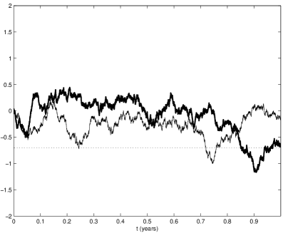
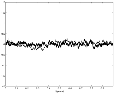
In Figures 1a)-3a) we show one trajectory of , , , solution of (5), (4), (3) when and one trajectory of , , , solution of (6), (7) for three different values of , that is for (Figure 1a)), (Figure 2a)) and (Figure 3a)). As suggested in [5] we choose , and we use the explicit Euler method with time step to integrate the initial value problems (5), (4), (3) and (6), (7) from time up to time , . Note that in Figures 1a)-3a) it is sufficient to represent one trajectory of , , , solution of system (5), (4), (3) to illustrate the behaviour of the corresponding trajectory of system (5), (4), (3). In fact the bank population considered is homogeneous and the processes , , , , behave all in the same way. As expected, increasing , that is increasing the rate of cooperation among banks, increases the “swarming” effect around the line of the trajectories of (5), (4), (3), and, as a consequence, decreases the number of defaults in the time interval , , increasing the stability of the system. In Figures 1a)-3a) the dotted line shows the default level .
Let us consider the loss distribution in the time interval , , i.e. the probability distribution of the random variable: number of bank defaults in the time interval , . In the model (5), (4), (3) when the loss distribution in , , is evaluated using statistical simulation starting from simulated trajectories of the model. Note that the loss distributions shown in Figures 1b)-3b) are computed using the definition of systemic risk (9) and using the assumptions about bank failure made in this paper. In Figures 1b)-3b) the dashed line shows the loss distribution in , , of system (1), (4), (3) when , while the solid line denotes the loss distribution of system (5), (4), (3) when and (see Figure 1b)), (see Figure 2b)) and (see Figure 3b)). Note that in the case of independent diffusion processes, i.e. when we consider system (1), (4), (3), or when we consider in (5), (4), (3), the loss distribution in , , is a binomial distribution with known parameters. When let us look more closely to the loss distribution in , , of the diffusion processes solution of (5), (4), (3) as a function of . This distribution is plotted with a solid line in Figures 1b)-3b). These distributions have a large mass near zero defaults together with a small, but not negligible, mass near defaults. These features of the loss distribution of (5), (4), (3) and their behaviour as functions of when increases show that the cooperation mechanism among banks present in (5), (4), (3) increases the stability of the individual bank, however it increases also the probability of “extreme” systemic risk in the time interval , . This last fact is shown in Figure 4 where we zoom the right-bottom corner of Figure 1b)-3b). Figure 4 shows that the “tail” of the loss distribution raises when increases.
Note that the different definitions of systemic risk used in [5] (i.e. (10)) and in this paper (i.e. (9)) do not change the qualitative behaviour of the systemic risk probability as a function of shown in Figures 1-4.
 a)
a)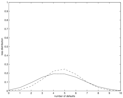 b)
b)
 a)
a)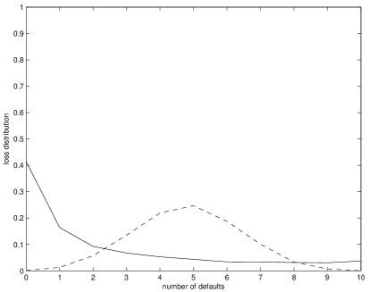 b)
b)
 a)
a)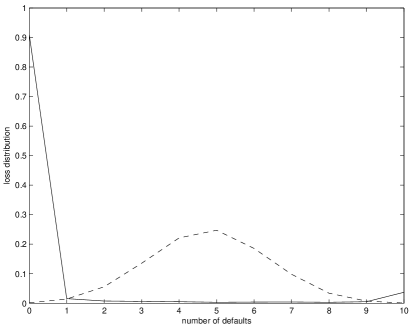 b)
b)
 a)
a) b)
b)
 c)
c)
3 A banking system model with two cooperation mechanisms
Let us introduce the banking system model studied in this paper. The log-monetary reserves as functions of time of the banks present in the banking system are modeled by the diffusion processes , , . These diffusion processes are defined implicitly through an initial value problem for a system of stochastic differential equations. In the model we use the cooperation mechanism present in (5) to describe the inter-bank borrowing and lending activity, and we introduce a new cooperation mechanism to describe the borrowing and lending activity between banks and monetary authority. This last mechanism depends from the difference as function of time between the empirical mean of the log-monetary reserves of the banks and a target trajectory , , chosen by the monetary authority that represents the log-monetary reserves of the “ideal bank” as a function of time.
Given , , , we begin modeling the dynamics of the log-monetary reserves of the banks with the following system of stochastic differential equations:
| (12) |
with the initial condition:
| (13) |
where , , is a continuous piecewise differentiable function and , . The initial value problem (12), (13) is completed with the assumption (3). Note that with abuse of notation in (13) is a random variable concentrated in the point , with probability one. We assume and , , where is the default barrier.
In (12) the parameter regulates the first cooperation mechanism expressed by the terms , , that controls the inter-bank borrowing and lending activity (see Section 2). The term , , of (12) is a part of the intervention of the monetary authority in the banking system dynamics and is responsible for the fact that the drift terms , , stabilize the trajectories of , , around , , instead than around , , as done in (5), (4) where we have (see Section 2). In (12) the parameter regulates the second cooperation mechanism expressed by the term , , added to the -th equation, . That is controls the strength of mean reversion of the empirical mean of the log-monetary reserves of the banks to the target trajectory of the log-monetary reserves of the “ideal bank” , . Equations (12) through the term proportional to impose that the mean of the log-monetary reserves of the banks of the system (i.e. , ) reverts to the log-monetary reserves of the “ideal bank” (i.e. , ). In the model (12), (13), (3) the bank population is homogeneous and when goes to infinity each bank behaves like the mean bank. That is the target trajectory , , represents the “ideal” log-monetary reserves of each bank and , , represents the “ideal” target trajectory of the log-monetary reserves of the banking system. The parameter controls the rate of the borrowing and lending activity between banks and monetary authority. That is the second cooperation mechanism of the model is regulated by and stabilizes the empirical mean of the diffusion processes , , along the target trajectory , . In fact the term , , of (12) can be rewritten as , .
Let us derive the mean field approximation of the banking system model (12), (13), (3). First of all let us rewrite the system of equations (12) as follows:
| (14) |
Summing the equations (14) for going from to , and dividing the resulting equation by N we have:
| (15) |
Let
| (16) |
be the empirical mean of the processes , . Equation (15) can be rewritten as follows:
| (17) |
The assumption (3) and the strong law of large numbers imply that:
| (18) |
Let , , be the limit as goes to infinity of the empirical mean , , and , be the process representing the log-monetary reserves of the “mean-bank” of the banking system model (12), (13), (3) in the limit goes to infinity. The mean field approximation of the dynamical system (12), (13), (3) can be deduced immediately from (14), (17). In fact when goes to infinity from (14), (17) we have:
| (19) | |||
| (20) | |||
| (21) |
The initial value problem (19), (20), (21) is the mean field approximation of the dynamical system (12), (13), (3). Note that equations (20) and (21) imply that , , therefore in (19) is multiplied by zero. This means that the choice of does not influence the trajectories of (19). That is the second cooperation mechanism introduced in (12) does not contribute to the mean field approximation (19), (20), (21) of (12), (13), (3). This is undesirable since we want to use the mean field approximation (19), (20), (21) to determine the parameters , that must be used to govern the banking system model (12), (13), (3). To avoid this inconvenience let us modify the banking system model (12), (13), (3). Starting from the target trajectory , , we introduce two auxiliary target trajectories , , , such that , , obtained from , , with a “slight” perturbation. For example, given , we choose , , , as follows:
| (22) |
We replace (12), (13) with the system of stochastic differential equations:
| (23) |
with the initial condition:
| (24) |
where, with abuse of notation, denotes a random variable concentrated in the point with probability one. The initial value problem (23), (24) is completed with the assumption (3).
The system of equations (23), (24), (3) is the banking system model with two cooperation mechanisms studied in this paper. The two cooperation mechanisms of model (23), (24), (3) are the same of those of model (12), (13), (3). However in model (23), (24), (3) the inter-bank borrowing and lending mechanism, governed by , stabilizes the system around the trajectory , , and the banks-monetary authority borrowing and lending mechanism, governed by , stabilizes the system around the trajectory , , and we have , .
Proceeding as done previously in the study of model (12), (13), (3) it is easy to see that the mean field approximation of the dynamical system (23), (24), (3) is:
| (25) | |||
| (26) | |||
| (27) |
where , is a stochastic process that represents the time evolution of the log-monetary reserves of the “mean-bank” of model (23), (24), (3) and , is an auxiliary variable.
For simplicity we use the same variables , , , , , to denote the dependent variables of the models (12), (13), (3) and (23), (24), (3) and of the corresponding mean field equations (19), (20), (21) and (25), (26), (27).
Let us point out that the models (12), (13), (3) and (23), (24), (3) can both be governed using (25), (26), (27). In fact instead of (23), (24), (3) we can consider (12), (13), (3) as banking system model and we can use the mean field equations (25), (26), (27) as shown in Section 4 to govern (12), (13), (3). We prefer to choose (23), (24), (3) as banking system model since with this choice the banking system model is governed through its mean field equations. Model (12), (13), (3) can be governed with the method presented in Section 4 through the auxiliary dynamical system (25), (26), (27) but cannot be governed using its mean field approximation (19), (20), (21) since in (19) is multiplied by zero.
For later purposes in the banking system model (23), (24), (3) and in its mean field approximation (25), (26), (27) from now on we allow the parameters and to be functions of time. That is in (23), (24), (3) and in (25), (26), (27) we assume:
| (28) |
It is easy to see that the functioning of the two cooperation mechanisms present in (23), (24), (3) remains unchanged when we consider , , to be functions of time.
Instead of choosing , , and the monetary authority can choose an interval of the real axis as function of time, that is the interval , , defined by two target trajectories , , , such that , . In this case , , can be defined as the arithmetic mean of , , .
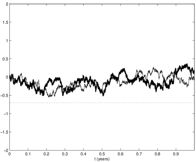
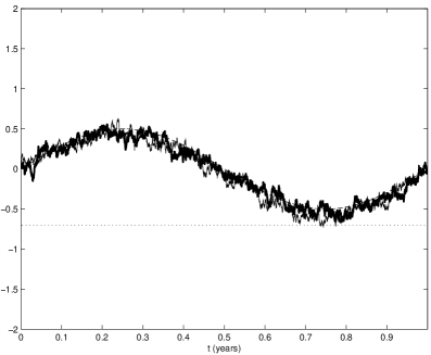
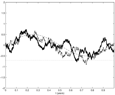
Figures 5a)-7a) show one trajectory of , , , solution of model (23), (24), (3), and one trajectory of , , , solution of the initial value problem (25), (26), (27), when , , , , and the constants , are chosen as follows: (see Figure 5a)), , (see Figure 6a)) and , (see Figure 7a)). As done in Section 2 we choose , , and we use the explicit Euler method with time step to integrate numerically the stochastic differential models (23), (24), (3) and (25), (26), (27), for , . In Figures 5a)-7a) the dotted line shows the default level , the dashed line shows the target trajectory , , . In Figures 5a)-7a) we show only one trajectory of , , , solution of model (23), (24), (3) since the bank population described by (23), (24), (3) is homogeneous and the processes , , , , behave all in the same way.
Let us study the loss distribution in the time interval , , of the diffusion processes solution of (23), (24), (3), that is let us consider the probability distribution of the random variable: number of bank defaults in the time interval , . The loss distribution in , , is evaluated using statistical simulation on a set of numerically generated trajectories of (23), (24), (3). In Figures 5b)-7b) the dashed line represents the loss distribution of the independent diffusion processes solution of (1), (4), (3) when , that is of the solution of system (23), (24), (3) when , , , , , , while the solid line represents the loss distribution of the diffusion processes solution of system (23), (24), (3) when , , , , , for the following values of the parameters and : (Figure 5b)), (Figure 6b)) and (Figure 7b)).
Figures 5-7 show how the banking system model (23), (24), (3) is stabilized by the two cooperation mechanisms discussed previously. In particular Figures 5-7 show the different effects of these two mechanisms. When and are constants and dominates over , that is when , (see Figure 5) we are in a situation similar to the situation discussed in Section 2 for the Fouque and Sun model (5), (4), (3) and presented in Figures 1-3. In this case the effect of the borrowing and lending activity among banks is dominant. This mechanism when increases improves the stability of the individual bank at the expense of an increased probability of extreme systemic risk. Moreover Figure 5 shows the “swarming effect” along the trajectory , , , induced by the term in (23). When and are constants and dominates over , that is when (see Figure 7) the effect of the borrowing and lending activity between banks and monetary authority is dominant. This mechanism stabilizes the empirical mean of the log-monetary reserves of the banks along the trajectory , , , without changing substantially the probability of systemic risk. This stabilization effect increases when increases. Note that the stabilization of the empirical mean of the log-monetary reserves of the banks around a “safe” target trajectory is useful to protect the banking system from systemic failures. In fact empirical mean of the log-monetary reserves of the banks stabilized around a “safe” target trajectory means that if there is a failed bank (i.e. a bank with log-monetary reserves below the “safe” target trajectory and in fact below the default level) there must be a bank or a group of banks that are “prosperous” (i.e. banks with log-monetary reserves above the “safe” target trajectory). In this situation it is possible for a prosperous bank or for a consortium of prosperous banks to rescue the failed one or the failed ones. In the intermediate cases, that is when is of the same order of magnitude of (see Figure 6) the effects of the two mechanisms are balanced.
It is easy to understand that given the default level raising the target trajectory , , (i.e. increasing , ) decreases the probability of systemic risk in a bounded time interval. However raising the target trajectory has the consequence of raising the log-monetary reserves of the banks. This fact discourages economic activity. Note that the loss of economic activity induced by the raise of , , is an undesired effect not considered in our model. Similarly decreasing the target trajectory , , (i.e. decreasing , ) increases the probability of systemic risk in a bounded time interval and has the consequence of decreasing the log-monetary reserves of the banks. We conclude that the monetary authority must pursue the goal of avoiding systemic failures keeping the log-monetary reserves of the banks as small as possible.
 a)
a)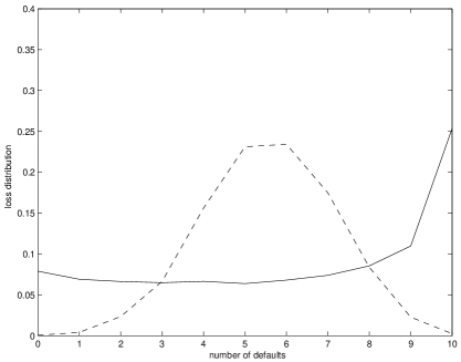 b)
b)
 a)
a)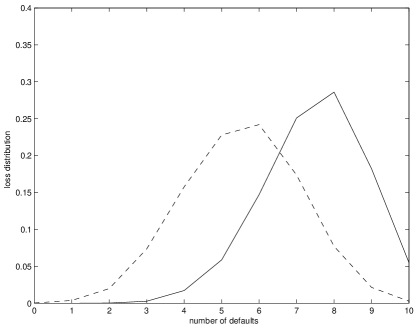 b)
b)
 a)
a)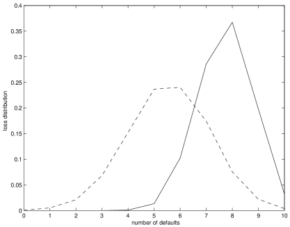 b)
b)
4 An optimal control problem for the mean-field equations
Let be the set of positive real numbers. Note that both the mean field equation (6) of the banking system model (5), (4), (3) and the mean field equation (25) of the banking system model (23), (24), (3) are of the form:
| (29) |
where the function is a sufficiently regular function. In fact the choices and
| (30) |
reduce (29) to (6), similarly the choices and
| (31) |
where , , and , , is defined by (26), (27) reduce (29) to (25). Finally note that the choices and
| (32) |
where , is defined by (20), (21) reduce (29) to (19). However, as already seen in Section 3, equations (20), (21) imply , and this means that in (32) is multiplied by zero.
Let be the set of the real square integrable processes defined in , . A real stochastic process , belongs to if and only if .
Given the constants , , and the target trajectory , , let us determine as solution of the following stochastic optimal control problem:
| (33) |
where
| (34) |
subject to the constraints:
| (35) | |||
| (36) |
In the control problem (33), (34), (35), (36) the function , is the utility function and , is the control variable.
The utility function , defined in (34) is the sum of two terms. The first term, penalizes the departure of , , from the target trajectory , . The second one, , penalizes the “size” of the control variable , .
We solve problem (33), (34), (35), (36) using the dynamic programming principle (see [10]). That is let
| (37) |
be the value function of the control problem (33), (34), (35), (36). The function , , satisfies the following Hamilton, Jacobi, Bellman equation (see [10]):
| (38) |
with final condition:
| (39) |
where
| (40) |
is the Hamiltonian function of the optimal control problem (33), (34), (35), (36).
Using (40) equation (38) becomes:
| (41) |
with the final condition (39).
From the knowledge of the value function solution of (41), (39) we determine the optimal control , solution of (33), (34), (35), (36) using the condition:
| (42) |
where , , is the solution of (35), (36) when =, is given by (42).
Proposition 1 reduces the solution of (41), (39) to the solution of a final value problem for a system of ordinary differential equations.
Proposition 1. A solution of problem (41), (39) is given by:
| (43) |
where the functions , , , are solution of the following final value problem for a system of Riccati ordinary differential equations:
| (44) | |||
| (45) | |||
| (46) |
The optimal control , , solution of problem (33), (34), (35), (36) determined by the value function (43) is:
| (47) |
Proof. Let , be of the form (43) (see [10]),
substituting (43) in (41), (39) and using the polynomial identity principle it is easy to see that problem (41), (39) reduces to the final value problem (44), (45), (46). Equation (47)
for the optimal control of problem (33), (34), (35), (36) follows from (43), (42).
Note that the constraint (35) of the optimal control problem (33), (34), (35), (36) is a model equation that can represent the mean field equations (6) or (25) when we have respectively or and equations (30) or (31) hold. Problem (33), (34), (35), (36) is the optimal control problem for the mean field approximation (25), (26), (27) of (23), (24), (3) used to control the behaviour of the trajectories of the banking system model (23), (24), (3). In fact we determine the functions , , that must be substituted in (23), (24), (3) to force the trajectories of (23), (24), (3) to swarm around , , from the optimal control (47) of problem (33), (34), (35), (36) imposing , and (31). Comparing the optimal control (47) with equation (31) when , and using the polynomial identity principle we have:
| (48) | |||
| (49) |
Note that the function , , is defined by the equations (26), (27) and contains an integral that depends from , . This means that equation (49) is an integral equation in the unknown , . The conditions , , imposed in (28) are constraints that must be satisfied. When they are not satisfied by the choices of , , made in (48), (49) they must be enforced. Let us point out that in the numerical experiments discussed in Section 5 the function , , determined by (48) is always positive while the function , , determined by (49) is not always smaller or equal than zero. When the function determined by (49) is positive, we enforce the choice to guarantee (28). More in general the enforcement of the constraints (28) can be done solving the equations (48), (49) in the least squares sense after imposing (28) as a constraint. The choice of , , , that follows from (48), (49), (28) induces a swarming effect of the trajectories of (23), (24), (3) around the target trajectory , , similar to the swarming effect induced by the optimal control soultion of (33), (34), (35), (36) on the trajectories of (35), (36).
Note that the polynomial identity principle can be used when we compare (47) with (31) but cannot be used if we compare (47) with (30) or with (32). In this last case this is due to the fact that in (32) is multiplied by zero. In fact in (30) and (32) is a polynomial of degree one respectively in and in with only one coefficient that can be chosen. This is the reason to consider model (23), (24), (3) instead of model (12), (13), (3).
Note that proceeding as done previously a possibly high dimensional dynamical system (i.e. the banking system model (23), (24), (3)) is controlled using a law (i.e. the law (48), (49), (28)) deduced from the solution of a control problem (i.e. problem (33), (34), (35), (36)) for a low dimensional dynamical system (i.e. the mean field equations (25), (26), (27) of the banking system model (23), (24), (3)).
The possibility, exploited here, of governing a high dimensional dynamical system using its mean field approximation, is based on the fact that in the problem considered the population of agents (i.e. the population of banks) described by the high dimensional dynamical system is homogeneous (i.e. the banks are all equal and in the limit goes to infinity all the banks behave like the mean bank). This feature of the banking system model (23), (24), (3) is a rather common feature that is found in many other circumstances in science and engineering.
5 Systemic risk governance
Let we consider in the model (23), (24), (3) the problem of governing the probability of systemic risk in the bounded time interval . The systemic risk governance is based on the choice of the target trajectory , , and of the parameter . The governance exploits the solution of the control problem (33), (34), (35), (36), and its relation with the banking system model (23), (24), (3) when the functions , , are chosen as suggested by (48), (49), (28). The goal of the governance is to keep the probability of systemic risk in the time interval , , between two given thresholds. Given this goal is pursued choosing at time the target trajectory , . In fact we know that increasing , , the systemic risk probability in decreases and that decreasing , , the systemic risk probability in increases.
Going into details given , the thresholds , such that and we want to determine a target trajectory , , such that the probability of systemic risk in the time interval satisfies the following inequalities:
| (50) |
Let us define some simple rules that can be used to choose , . At time the “simplest” choice for the target trajectory in the time interval is , . In correspondence to this choice the monetary authority determines the functions , , , using (48), (49), (28) and evaluates the probability of systemic risk in the time interval associated to the choices of , , , done, that is evaluates . Note that depends not only from , , , , but also from the values taken by the variables , . Based on the value of the monetary authority acts as follows:
-
Strategy 3: if the monetary authority leaves the target trajectory chosen, that is , , unchanged.
Let us discuss some numerical experiments that illustrate a simple implementation of the previous strategies. In the numerical experiments we present the simulation of the governance of the systemic risk in the next year during a period of two years. The governance takes place quarterly and consists, at the beginning of each quarter, in choosing the target trajectory of the log-monetary reserves of the “ideal bank” in the next year and in translating this choice in rules for the banks determining the values of the functions , in the next year using (48), (49), (28). These choices are done pursuing the goal of enforcing the probability of systemic risk in the next year to satisfy the inequalities (50). For simplicity we restrict the choice of the target trajectory to a finite set of functions constructed with some simple rules.
In the first numerical experiment we study the governance of the probability of systemic risk in the next year when there are no shocks acting on the banking system. In the second and in the third numerical experiment we study the governance of the probability of systemic risk in the next year in presence of positive and negative shocks acting on the banking system. These shocks are represented as abrupt changes of , that is we consider , , to be a piecewise constant function.
Numerical experiment 1. We choose a time horizon of three years, that is , and the time step of the governance decisions , that is we take systemic risk governance decisions quarterly. In the time interval we consider the time intervals , , where and , . The remaining parameters of the model used in the numerical example are: , , , , , , , . Note that in this experiment we have , , . The choice of constant volatility corresponds to the fact that there are no shocks acting on the banking system during the time interval considered. In the numerical experiments the number of banks is constant during the time evolution, that is there are no bank defaults during the time evolution.
In each time interval , the model (23), (24), (3) reduces to:
| (51) |
with initial condition:
| (52) |
and
| (53) |
As explained in Section 2, for , the probability of systemic risk in the time interval in the model (51), (52), (53) is evaluated using statistical simulation starting from trajectories of (51), (52), (53) generated numerically. These trajectories are obtained integrating (51), (52), (53) using the explicit Euler method with time step .
For in order to keep the probability of systemic risk in the time interval between the thresholds and , we give to the monetary authority eight choices of target trajectory that push the trajectories of the -th model (51), (52), (53) “downward” and eight choices of target trajectory that push the trajectories of the -th model (51), (52), (53) “upward”. Finally the monetary authority has the possibility of choosing the target trajectory constant during the next year and equal to its value at the decision time. This last choice leaves the trajectories of the -th model (51), (52), (53) “unchanged”, that is it does not push them “upward” or “downward”. The piecewise linear functions listed in (56) are the target trajectories used to implement these choices.
Initially, for simplicity, starting from , , the monetary authority chooses , as target trajectory. For , given the time interval , the monetary authority assumes , , and evaluates . Depending from the value of the monetary authority acts as suggested by Strategy 1-Strategy 3. This last step is done choosing one of the following target trajectories:
| (56) | |||
| (57) |
Note that in (56) when (respectively ) the target trajectory is a non decreasing (respectively non increasing) piecewise linear function. When the target trajectory is constant. Recall that we are always assuming that , , and that choices of target trajectories defined in (56) that violate this constraint are not considered. That is when the monetary authority chooses a target trajectory with in the time interval the trajectories of the banking system model (51), (52), (53) move “upward” and the probability of systemic risk in the next year decreases, vice versa when the monetary authority chooses a target trajectory with in the time interval the trajectories of the banking system model (51), (52), (53) move “downward” and the probability of systemic risk in the next year increases. Finally when the monetary authority chooses the target trajectory in the time interval , the character of the trajectories of the banking system model (51), (52), (53) is left unchanged and the corresponding probability of systemic risk in the next year is left approximately unchanged.
Note that the choices made in (56) are only illustrative. Many other choices of target trajectories are possible to implement Strategy 1-Strategy 3.
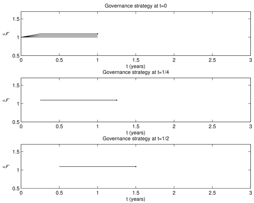
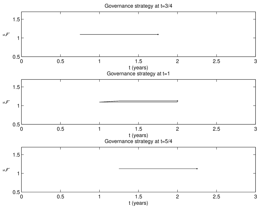
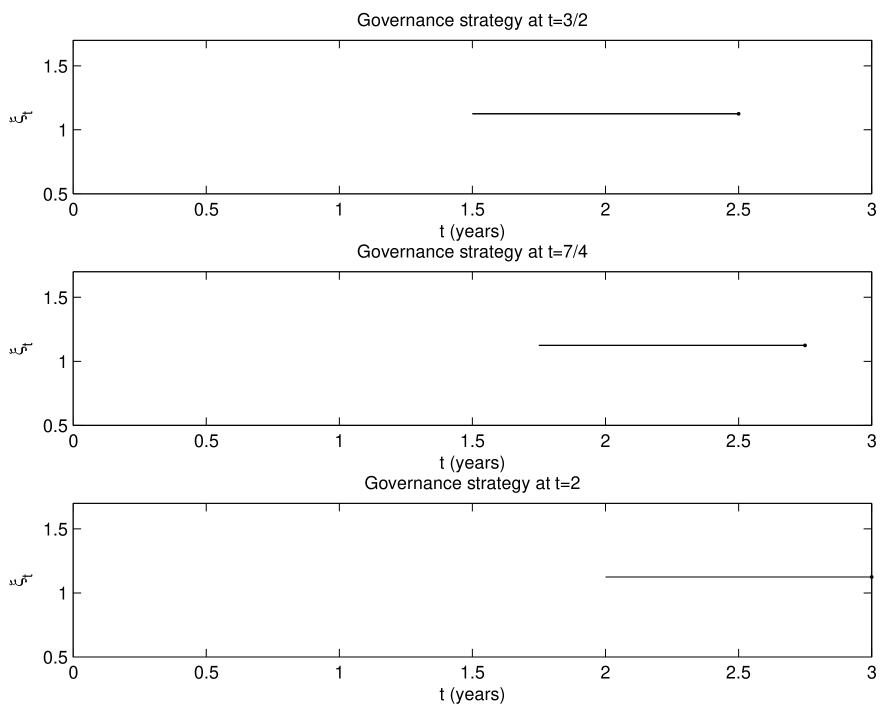
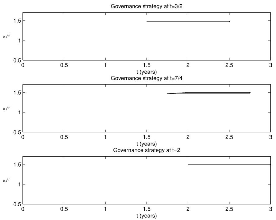
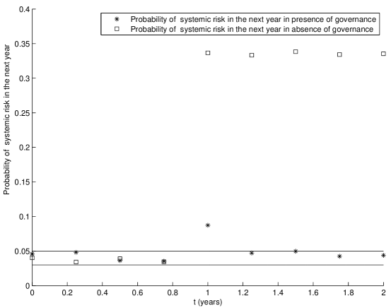
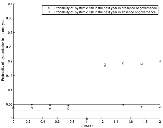
In Figures 8-10 we show the governance of model (51), (52), (53) made by the monetary authority at the beginning of each quarter pursuing the goal of keeping the probability of systemic risk in the next year between the thresholds and . In Figures 8-10 the choices of target trajectories considered at the beginning of each quarter by the monetary authority in the decision making process are shown. The target trajectory marked with a dot at its endpoint is the final choice of target trajectory made by the monetary authority. The monetary authority runs through the possible choices of target trajectories listed in (56) in their natural order according to Strategy 1-Strategy 3 starting from the choice and evaluates the probability of systemic risk in the next year associated to each target trajectory considered before making its final decision (see Figures 8-10). The first target trajectory encountered that has the associated probability of systemic risk in the next year that satisfies (50) is chosen. Figure 11 shows the probability of systemic risk in the next year evaluated at the beginning of each quarter during the time interval both in presence and in absence of governance. In presence of governance the probability shown is the probability of systemic risk in the next year evaluated at the beginning of each quarter when the target trajectory chosen is the final choice made by the monetary authority in that quarter marked with a dot at its endpoint in Figures 8-10. In absence of governance we choose , , , , , , and we evaluate the probability of systemic risk in the next year at the beginning of each quarter. The choices made in absence of governance guarantee that the probability of systemic risk in the next year at time is between the given thresholds.
Recall that in the Numerical experiment 1 we have , , . Figures 8-10 show that, when the volatility is constant in the time interval , , the systemic risk governance of the monetary authority is reduced to the choice of the target trajectory at the beginning of the time interval considered, that is at time . When this choice is done correctly continuing with a constant target trajectory or with small variations of it in each successive time interval , , is sufficient to keep the probability of systemic risk in the next year between the given thresholds. Figure 11 shows that, when the volatility is constant in the time interval , , the presence or absence of governance does not make a significant difference provided that in absence of governance a good choice of the target trajectory and of the values of the parameter and is done at time .
In the next experiments we consider two examples of non constant volatility in the time interval , , that is we consider the case when there are shocks acting on the banking system during the time interval considered.
Numerical experiments 2 and 3.
The setting of the Numerical experiments 2 and 3 is the same one of Numerical experiment 1 except for the fact that in these two experiments the volatility is not constant. We allow abrupt changes of volatility to model shocks acting on the banking system.
In Numerical experiment 2 we choose the volatility as follows:
| (60) |
In Numerical experiment 3 we choose the volatility as follows:
| (64) |
The function (60) models a positive volatility shock, while the function (64) models a negative volatility shock followed by a positive one.
Note that in the Numerical experiments 2 and 3 at the beginning of each quarter the monetary authority in the process of making its decision about systemic risk governance assumes that the volatility in the next year is constant at its present value. That is the monetary authority does not foresee the volatility shocks, simply reacts to them when they occur.
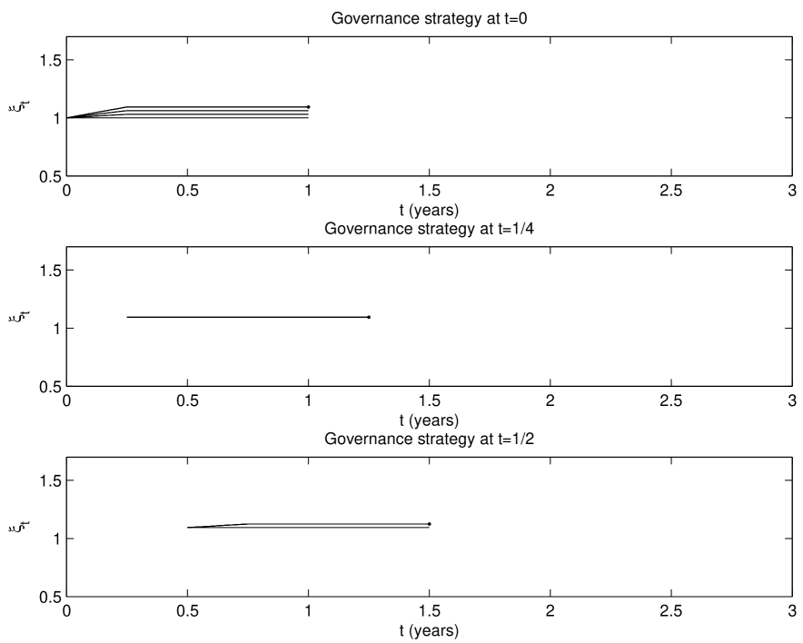
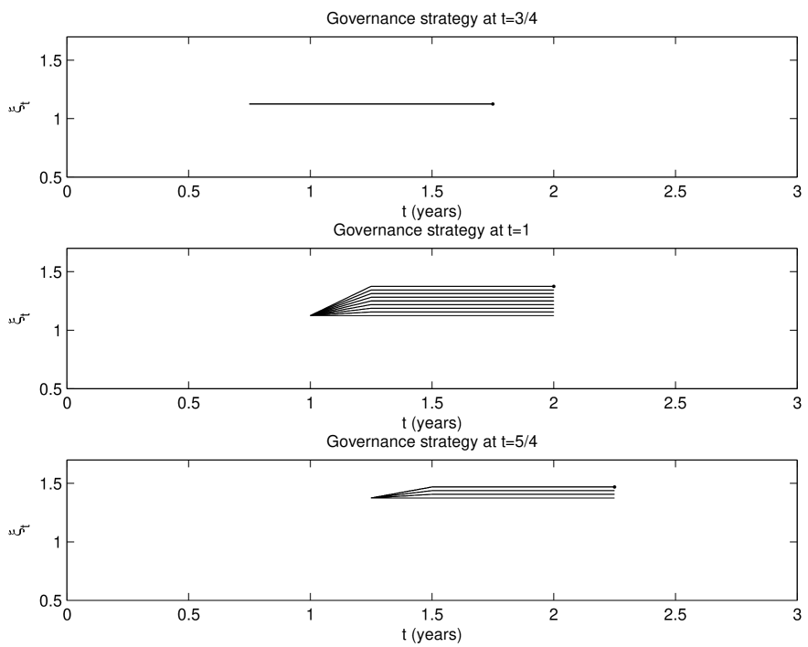
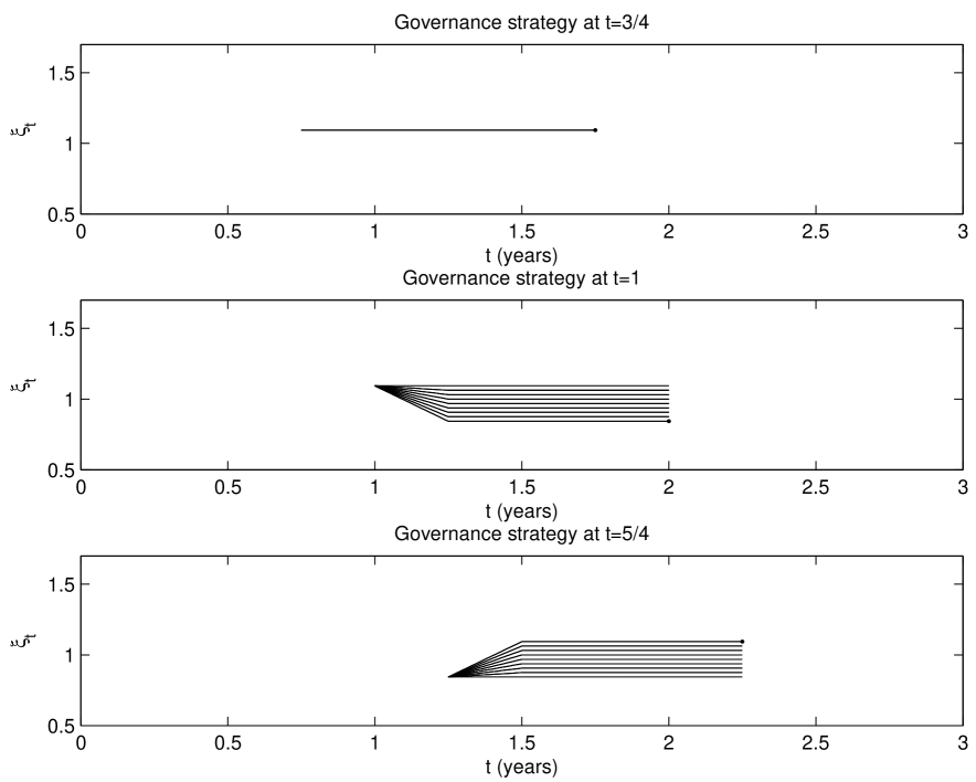
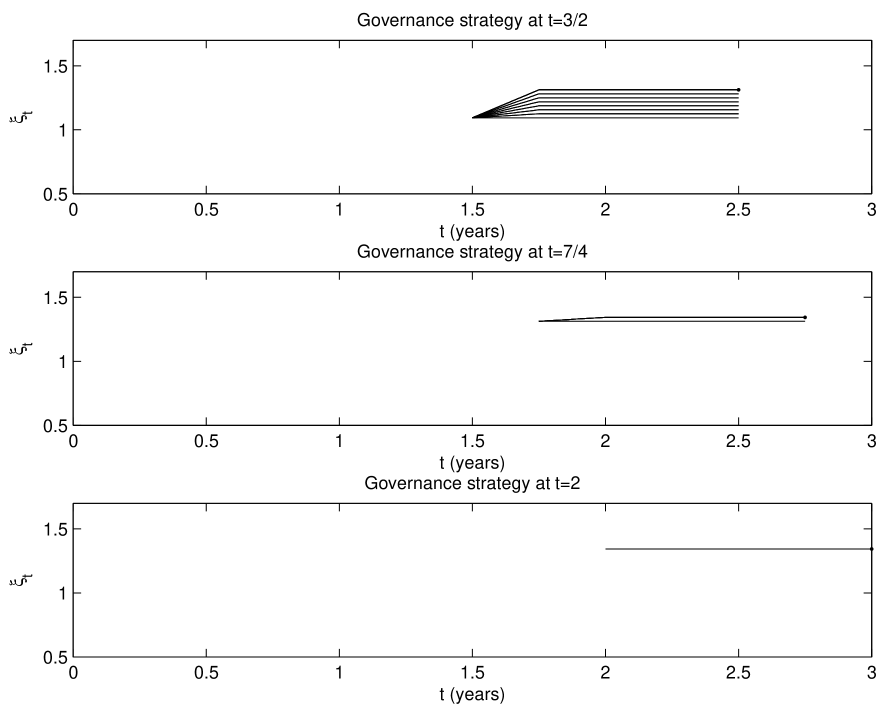
Figures 12-14 show the governance of the banking system model (51), (52), (53) in the time interval , , made by the monetary authority at the beginning of each quarter in order to keep the probability of systemic risk during the next year between the thresholds and when the volatility is given by (60). Figures 16-18 show the same quantities of Figures 12-14 when the volatility is given by (64). In particular in each image of Figures 12-14 and of Figures 16-18 we show the choices of the target trajectories for the next year considered by the monetary authority at the beginning of each quarter and the final choice of the target trajectory for the next year made at the beginning of each quarter (marked with a dot at its endpoint). Figure 15 and 19 show respectively in the time interval the probability of systemic risk in the next year evaluated at the beginning of each quarter both in presence and in absence of governance for the Numerical experiments 2 and 3. In absence of governance as done in Numerical experiment 1 we have chosen: , , , , , .
Figures 12-19 show that, as expected, the governance of the systemic risk in presence of positive and/or negative volatility shocks is more demanding than in absence of volatility shocks. Nevertheless Figures 12-19 show that the elementary systemic risk governance outlined in this Section after a few adjustments is able to keep the probability of systemic risk in the next year between the assigned thresholds.


References
- [1] S. Battiston, D.D. Gatti, M. Gallegati, B.C. Greenwald, J.E. Stiglitz, Liaisons dangereuses: increasing connectivity, risk sharing, and systemic risk, Journal of Economic Dynamics and Control, 36(8), pp. 1121-1141, 2012.
- [2] N. Beale, D.G. Rand, H. Battey, K. Croxson, R.M. May, M.A. Nowak, Individual versus systemic risk and the Regulator’s Dilemma, Proceedings of the National Academy of Sciences, 108 (31), pp. 12647-12652, 2011.
- [3] D. Bisias, M. Flood, A. Lo, S. Valavanis, A survey of systemic risk analytics, Annual Review of Financial Economics, 4, pp. 255-296, 2012.
- [4] R. Carmona, J.P. Fouque, L.H. Sun, Mean field games and systemic risk, Communications in Mathematical Sciences, 13(4), pp. 911-933, 2015.
- [5] J.P. Fouque, L.H. Sun, Systemic risk illustrated, in Handbook of Systemic Risk, J.P. Fouque, J. Langsam Editors, Cambridge University Press, Cambridge, U.K., 2013, pp. 444-452.
- [6] G. Gallavotti, Statistical Mechanics: A Short Treatise, Springer Verlag, New York, 1999.
- [7] J. Garnier, G. Papanicolaou, T.W. Yang, Large deviations for a mean field model of systemic risk, SIAM Journal on Financial Mathematics, 4, pp. 151-184, 2013.
- [8] A.G. Haldane, R.M. May, Systemic risk in banking ecosystems, Nature, 469, pp. 351-355, 2011.
- [9] Handbook of Systemic Risk, J.P. Fouque, J. Langsam Editors, Cambridge University Press, Cambridge, U.K., 2013.
- [10] G.E. Kolosov, Optimal Design of Control Systems: Stochastic and Deterministic Problems, CRC Press, New York, 1999.
- [11] R.M. May, N. Arinaminpathy, Systemic risk: the dynamics of model banking systems, Journal of the Royal Society Interface, 7, pp. 823-838, 2010.
- [12] E. Nier, J. Yang, T. Yorulmazer, A. Alentorn, Network models and financial stability, Journal of Economic Dynamics and Control, 31, pp. 2033-2060, 2007.