A minimal HIV-AIDS infection model with general incidence rate
and application to Morocco data

Abstract

We study the global dynamics of a SICA infection model with general incidence rate. The proposed model is calibrated with cumulative cases of infection by HIV–AIDS in Morocco from 1986 to 2015. We first prove that our model is biologically and mathematically well-posed. Stability analysis of different steady states is performed and threshold parameters are identified where the model exhibits clearance of infection or maintenance of a chronic infection. Furthermore, we examine the robustness of the model to some parameter values by examining the sensitivity of the basic reproduction number. Finally, using numerical simulations with real data from Morocco, we show that the model predicts well such reality.

AMS 2010 subject classifications 34D23, 92D30.

1 Introduction

Human immunodeficiency virus or HIV, is a type of virus that can cause a disease called acquired immunodeficiency syndrome, or AIDS. HIV infection affects the immune system, which is body’s natural defence against diseases. If left untreated, serious illness can occur. Normally innocuous infections, such as influenza or bronchitis, can then get worse, become very difficult to treat, or even cause death. In addition, the risk of cancer is also increased. For this reason, the World Health Organization is committed to end the AIDS epidemic by 2030 [35].

According to the latest statistics on the state of AIDS epidemic by UNAIDS [35], 36.9 million people, globally, were living with HIV in 2017, of which 21.7 million individuals were accessing ART (antiretroviral therapy) treatment; and 1.8 million became newly infected with HIV in 2017. A total of 77.3 million individuals have become infected with HIV since the start of the epidemic in 1981. Figures of death indicate that 940,000 people died of AIDS-related illnesses in 2017, with a total of 35.4 million people that have died from AIDS-related illnesses since the start of the epidemic.

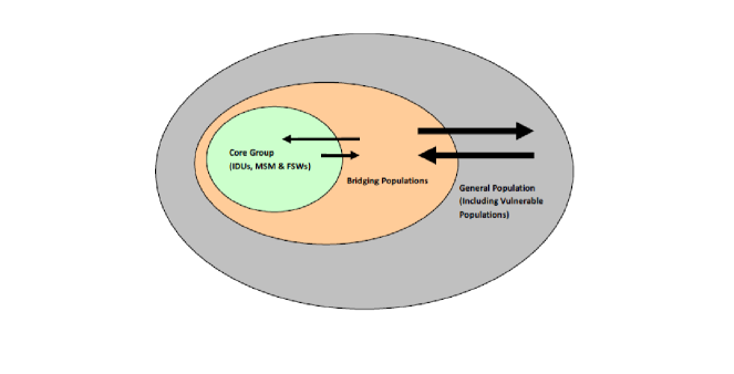
The risk of HIV infection depends on the mode of transmission, the prevalence of HIV and the behaviour of the population. Human populations exhibit highly variable behaviours in terms of sex and injecting drug use, a heterogeneity of risk conceptualized by convention across three population groups (see Figure 1). The key group is those most exposed to HIV infection, generally injecting drug users, men who have sex with men (including sex workers) and sex workers. The second group is the gateway population (e.g., truck drivers and clients of sex workers) who pose a risk of intermediate exposure and puts the high-risk group in contact with the third low-risk group, general population, which brings together the bulk of the population of all communities.

Figure 1: Heterogeneity of the exposed risk to a sexually transmitted infection in a given population.

Morocco, officially the Kingdom of Morocco, is a unitary sovereign state located in North-western Africa that has a population of 34 996 167. The political regime of Morocco is a constitutional monarchy. Moroccan culture is a blend of Berber, Arab, West African and European influences. Its geographical proximity to Europe and its diverse cultures make it among the most visited destinations with a ranking of 33rd out of 227 countries [28]. In 2016, Morocco had more than 1000 new HIV infections and almost 1000 AIDS-related deaths. There were 22 000 people living with HIV in 2016, among whom 48% were accessing ART treatment. In 2018, Morocco began its thirtieth year of response to HIV, with great satisfaction. Concerted efforts in the country have resulted in a 42% decline in new HIV infections since 2010, well above the only 4% decrease in the Middle East and North Africa. Coverage of HIV treatment has also increased in the country, from 16% in 2010 to 48% in 2016 [34].

In our study, we assume that HIV infected individuals, with and without symptoms, have access to ART treatment. The part of HIV infected individuals without AIDS symptoms move to the chronic stage (HIV-infected individuals under ART treatment with a low viral load) [32]. In this class, when they respect carefully the ART treatment and do not have a risky behaviour for HIV transmission, individuals have the same life expectancy as uninfected ones and the risk of HIV transmission is greatly reduced [8, 32, 33]. If the infected individuals do not take ART treatment, then they can transmit the infection and the symptoms will start to appear. We consider that these individuals are aware of their state of health, so they take precautions not to infect others, and/or are too sick to have a risky behaviour. Mathematically, this translates to the fact that function $f$ of model (1) depends only on $S$ and $I$. These reductionist assumptions have been made to reduce the epidemic problem to a mathematical tractable form. In order to contribute to the project of ending this epidemic by 2030, we need to predict the evolution of its behaviour, which is a highly challenging problem. One of the main tools to reach our goal is HIV infection mathematical modelling. For this, based on [33], we propose the following model:

$$\begin{cases}\dot{S}(t)=\Lambda-\mu S(t)-f\left(S(t),I(t)\right)I(t),\\[5.69046pt] \dot{I}(t)=f\left(S(t),I(t)\right)I(t)-(\rho+\phi+\mu)I(t)+\alpha A(t)+\omega C(t),\\[5.69046pt] \dot{C}(t)=\phi I(t)-(\omega+\mu)C(t),\\[5.69046pt] \dot{A}(t)=\rho\,I(t)-(\alpha+\mu+d)A(t),\end{cases}$$ (1)

with initial conditions

$$S(0)=S_{0}\geq 0,\ I(0)=I_{0}\geq 0,\ C(0)=C_{0}\geq 0,\ A(0)=A_{0}\geq 0.$$ (2)

The model considers a varying population size in a homogeneously mixing population and subdivides the human into four mutually-exclusive compartments:

• Susceptible individuals ($S$);

• HIV infected individuals with no clinical symptoms of AIDS (the virus is living or developing in the host but without producing symptoms or only mild ones), but that are able to transmit HIV to other individuals ($I$);

• HIV infected individuals under ART treatment with a viral load remaining low ($C$);

• HIV infected individuals with AIDS clinical symptoms ($A$).

The susceptible population is increased by recruitment of susceptible individuals at a rate $\Lambda$, while $\mu$ is the natural death rate of all individuals. The transmission process is governed by a general incidence function $f(S,I)$ [24]. Individuals in the class $I$ progress to the class $C$ at a rate $\phi$ and to the class $A$ at a rate $\rho$. Individuals in the class $A$, that start taking ART treatment, progress to the class $C$ at rate $\alpha$. Individuals in the class $C$ return to the class $I$, if the treatment is not maintained, at a rate $\omega$. Individuals suffer from AIDS induced death at a rate $d$. The total population at time $t$, denoted by $N(t)$, is given by

$$N(t)=S(t)+I(t)+C(t)+A(t).$$

As in [9, 13, 15, 14, 22], the incidence function $f(S,I)$ is assumed to be non-negative and continuously differentiable in the interior of $\mathbb{R}^{2}_{+}$ and satisfies the following hypotheses:

$$f(0,I)=0,\hskip 5.69046pt\text{ for all }I\geq 0, H_{1}$$ ()

$$\frac{\partial f}{\partial S}(S,I)>0,\hskip 5.69046pt\text{ for all }S>0\ \text{ and }\ I\geq 0, H_{2}$$ ()

$$\frac{\partial f}{\partial I}(S,I)\leq 0\hskip 5.69046pt,\hskip 5.69046pt\text{ for all }\ S\geq 0\ \text{ and }\ I\geq 0. H_{3}$$ ()

The reason for adopting hypothesis ($H_{3}$) is the fact that susceptible individuals take measures to reduce contagion if the epidemics breaks out. This idea has first been explored in [4].

The rest of the paper is structured as follows. The mathematical analysis of the model is presented in Section 2. Then we establish the stability of the equilibria in Section 3. A sensitivity analysis of the basic reproduction number is given in Section 4. Finally, in Section 5 an application of the model to HIV/AIDS infection data from the period of 1986–2015 in Morocco is provided, and some conclusions are derived in Section 6.

2 Basic results

In this section, we prove that all solutions with nonnegative initial data will remain nonnegative and bounded for all time.

Theorem 1.

All solutions of (1) starting from non-negative initial conditions (2) exist for all $t>0$ and remain bounded and non-negative. Moreover,

$$N(t)\leq N(0)+\dfrac{\Lambda}{\mu}.$$

Proof.

For positivity, we show that any solution starting in the non-negative set $\mathbb{R}^{4}_{+}=\{(S,I,C,A)\in\mathbb{R}^{4}:S\geqslant 0;\ I\geqslant 0;\ C\geqslant 0;\ A\geqslant 0\}$ remains there forever: $\big{(}S(t),I(t),C(t),A(t)\big{)}\in\mathbb{R}^{4}_{+}$. We have

$$\dot{S}\mid_{S=0} = \Lambda\geq 0,$$

$$\dot{I}\mid_{I=0} = \omega C+\alpha A\geq 0,$$

$$\dot{C}\mid_{C=0} = \phi I\geq 0,$$

$$\dot{A}\mid_{A=0} = \rho I\geq 0.$$

Hence, positivity of all solutions initiating in $\mathbb{R}^{4}_{+}$ is guaranteed. Now, we prove that the solutions are bounded. Adding the four equations of system (1), we get

$$\dot{N}(t) = \Lambda-\mu N(t)-dA(t),$$

$$\dot{N}(t) \leq \Lambda-\mu N(t),$$

and we deduce that

$$N(t)\leq N(0)e^{-\mu t}+\dfrac{\Lambda}{\mu}(1-e^{-\mu t}),$$

since $0\leq e^{-\mu t}\leq 1$ and $1-e^{-\mu t}\leq 1$. Thus,

$$N(t)\leq N(0)+\dfrac{\Lambda}{\mu}.$$

The proof is complete. ∎

It is easy to see that system (1) has a disease-free equilibrium $E_{f}=(\Lambda/\mu,0,0,0)$. Note that the trivial equilibrium with $(0,0,0,0)$ is not possible by hypothesis ($H_{1}$). Following the approach presented by van den Driessche and Watmough in [36], the basic reproduction number $R_{0}$ is obtained by calculating the spectral radius of the next-generation matrix for system (1). We get

$$R_{0}=\dfrac{f(\Lambda/\mu,0)\xi_{2}\xi_{3}}{\mathcal{D}},$$ (3)

where along all manuscript

$$\begin{split}\xi_{1}&=\rho+\phi+\mu,\\ \xi_{2}&=\omega+\mu,\\ \xi_{3}&=\alpha+\mu+d,\end{split}$$ (4)

and

$$\mathcal{D}=\mu[\xi_{2}(\xi_{3}+\rho)+\phi\xi_{3}+\rho d]+\rho\omega d.$$ (5)

Biologically, the basic reproduction number represents the average of new infected individuals produced by a single HIV-infected/AIDS individual on contact in a completely susceptible population.

Theorem 2.

(i) If $R_{0}\leq 1$, then the system (1) has a unique disease-free equilibrium of the form $E_{f}=(\Lambda/\mu,0,0,0)$.
(ii) If $R_{0}>1$, then the disease-free equilibrium is still present and the system (1) has a unique endemic equilibrium of the form $E^{*}(S^{*},I^{*},C^{*},A^{*})$, with $S^{*}\in\bigg{(}0,\dfrac{\Lambda}{\mu}\bigg{)}$, $I^{*}>0$, $C^{*}>0$ and $A^{*}>0$.

Proof.

Obviously, $E_{f}$ is the unique steady state of system (1) when $R_{0}\leq 1$. To find the other equilibrium of system (1), we solve the system

$$\begin{split}\Lambda-\mu S-f\left(S,I\right)I&=0,\\ f\left(S,I\right)I-\xi_{1}I+\alpha A+\omega C&=0,\\ \phi I-\xi_{2}C&=0,\\ \rho\,I-\xi_{3}A&=0,\end{split}$$ (6)

where $\xi_{i}$, $i=1,2,3$, are given as in (4). From (3) and (6), we get

$$C=\dfrac{\phi}{\xi_{2}}I\qquad\text{ and }\qquad A=\dfrac{\rho}{\xi_{3}}I.$$

Adding (1) and (2), we obtain

$$\Lambda-\mu S-\bigg{(}\xi_{1}-\dfrac{\omega\phi}{\xi_{2}}-\dfrac{\alpha\rho}{\xi_{3}}\bigg{)}I=0.$$

Then,

$$I=\dfrac{(\Lambda-\mu S)R_{0}}{f\big{(}\Lambda/\mu,0\big{)}}.$$

Now, we consider the following function defined on the interval $\bigg{[}0,\dfrac{\Lambda}{\mu}\bigg{]}$ by

$$G(S)=f\bigg{(}S,\dfrac{(\Lambda-\mu S)R_{0}}{f\big{(}\Lambda/\mu,0\big{)}}\bigg{)}-\xi_{1}+\dfrac{\omega\phi}{\xi_{2}}+\dfrac{\alpha\rho}{\xi_{3}}.$$

By using the intermediate value theorem on the function $G(S)$, we show that the second equation of system (6) admits a unique solution. Clearly, $G(0)=-\dfrac{\mathcal{D}}{\xi_{2}\xi_{3}}<0$ and $G(\Lambda/\mu)=\dfrac{\mathcal{D}}{\xi_{2}\xi_{3}}\big{[}R_{0}-1\big{]}$, with $\mathcal{D}$ as in (5), and

$$G^{\prime}(S)=\dfrac{\partial f}{\partial S}-\dfrac{\mu R_{0}}{f\big{(}\Lambda/\mu,0\big{)}}\dfrac{\partial f}{\partial I}>0.$$

By hypotheses ($H_{2}$) and ($H_{3}$), if $R_{0}>1$, then the system admits a unique endemic equilibrium $E^{*}(S^{*},I^{*},C^{*},A^{*})$ with $S^{*}\in\left(0,\dfrac{\Lambda}{\mu}\right)$, $I^{*}>0$, $C^{*}>0$ and $A^{*}>0$. This completes the proof. ∎

3 Stability analysis

In this section, we focus on the stability analysis of the equilibria. In the case of $R_{0}\leq 1$, we have:

Theorem 3.

The disease-free equilibrium $E_{f}$ is globally asymptotically stable if $R_{0}\leq 1$.

Proof.

To study the global stability of $E_{f}$ for system (1), we construct a Lyapunov functional at $E_{f}$ as follows:

$$V_{1}(S,I,C,A)=S-S_{0}-\int_{S_{0}}^{S}\frac{f(S_{0},0)}{f(X,0)}dX+I+\dfrac{\omega}{\xi_{2}}C+\dfrac{\alpha}{\xi_{3}}A,$$

where $S_{0}=\dfrac{\Lambda}{\mu}$ and $\xi_{i}$, $i=2,3$, are given as in (4). It is clear from hypothesis ($H_{2}$) that $V_{1}$ is non-negative. The time derivative of $V_{1}$ along the solution of system (1) is given by

$$\dfrac{dV_{1}}{dt} = \left(1-\dfrac{f(S_{0},0)}{f(S,0)}\right)\dot{S}+\dot{I}+\dfrac{\omega}{\xi_{2}}\dot{C}+\dfrac{\alpha}{\xi_{3}}\dot{A}$$

$$= \mu\left(1-\dfrac{f(S_{0},0)}{f(S,0)}\right)(S_{0}-S)+I\left[\dfrac{f(S,I)}{f(S,0)}f(S_{0},0)-\left(\xi_{1}-\dfrac{\omega\phi}{\xi_{2}}-\dfrac{\alpha\rho}{\xi_{3}}\right)\right]$$

$$= \mu\left(1-\dfrac{f(S_{0},0)}{f(S,0)}\right)(S_{0}-S)+\dfrac{\mathcal{D}}{\xi_{2}\xi_{3}}I\left(\dfrac{f(S,I)}{f(S,0)}R_{0}-1\right)$$

$$\leq \mu\left(1-\dfrac{f(S_{0},0)}{f(S,0)}\right)(S_{0}-S)+\dfrac{\mathcal{D}}{\xi_{2}\xi_{3}}I\left(R_{0}-1\right),$$

where $\mathcal{D}$ is given in (5) and $\xi_{i}$, $i=1,2,3$, are defined by (4). Using the inequalities

$$1-\dfrac{f(S_{0},0)}{f(S,0)} \geq 0\quad\text{for}\quad S\geq S_{0},$$

$$1-\dfrac{f(S_{0},0)}{f(S,0)} < 0\quad\text{for}\quad S<S_{0},$$

we have

$$\left(1-\dfrac{f(S_{0},0)}{f(S,0)}\right)(S_{0}-S)\leq 0.$$

Therefore, $\frac{dV_{1}}{dt}\leq 0$. Furthermore, the largest compact invariant set in $\left\{(S,I,C,A)\mid\frac{dV_{1}}{dt}=0\right\}$ is just the singleton $E_{f}$. Using LaSalle’s invariance principle [18], we conclude that $E_{f}$ is globally asymptotically stable. ∎

Now, we study the stability of the equilibria in the case $R_{0}>1$. For this, we assume that function $f$ satisfies the following condition:

$$\bigg{(}1-\dfrac{f(S,I)}{f(S,I^{*})}\bigg{)}\bigg{(}\dfrac{f(S,I^{*})}{f(S,I)}-\dfrac{I}{I^{*}}\bigg{)}\leq 0,\ \text{ for all }\ S,I>0. H_{4}$$ ()

Theorem 4.

(i) If $R_{0}>1$, then the disease-free equilibrium $E_{f}$ is unstable.
(ii) If $R_{0}>1$ and ($H_{4}$) holds, then the endemic equilibrium $E^{*}$ is globally asymptotically stable.

Proof.

We begin by proving the instability of $E_{f}$. For any arbitrary equilibrium $\overline{E}(\overline{S},\overline{I},\overline{C},\overline{A})$, the characteristic equation is given by

$$\begin{array}[]{ccc}\left|\begin{array}[]{cccc}-\mu-\dfrac{\partial f}{\partial S}\overline{I}-\lambda&-\dfrac{\partial f}{\partial I}\overline{I}-f(\overline{S},\overline{I})&0&0\\[8.0pt] \dfrac{\partial f}{\partial S}\overline{I}&\dfrac{\partial f}{\partial I}\overline{I}+f(\overline{S},\overline{I})-\xi_{1}-\lambda&\omega&\alpha\\[8.0pt] 0&\phi&-(\xi_{2}+\lambda)&0\\[8.0pt] 0&\rho&0&-(\xi_{3}+\lambda)\end{array}\right|&=&0,\end{array}$$

where $\xi_{i}$, $i=1,2,3$, are defined in (4). Evaluating the characteristic equation at $E_{f}(S_{0},0,0,0)$, we have

$$\lambda^{3}+a_{1}\lambda^{2}+a_{2}\lambda+a_{3}=0,$$

where

$$a_{1} = \xi_{1}+\xi_{2}+\xi_{3}-f(S_{0},0),$$

$$a_{2} = \xi_{1}\xi_{3}+\xi_{1}\xi_{2}+\xi_{2}\xi_{3}-(\xi_{2}+\xi_{3})f(S_{0},0)-\phi\omega-\rho\alpha,$$

$$a_{3} = (1-R_{0})\mathcal{D},$$

$\mathcal{D}$ as in (5). It is clear that $a_{3}<0$ when $R_{0}>1$. Then, the disease-free equilibrium $E_{f}$ is unstable. Now, we establish the global stability of the endemic equilibrium $E^{*}$. For that, we define a Lyapunov functional $V_{2}$ as follows:

$$V_{2}(S,I,C,A)=S-S^{*}-\displaystyle{\int_{S^{*}}^{S}}\frac{f(S^{*},I^{*})}{f(X,I^{*})}dX+I-I^{*}-I^{*}\ln\left(\dfrac{I}{I^{*}}\right)\\ +\dfrac{\omega}{\xi_{2}}\left(C-C^{*}-C^{*}\ln\left(\dfrac{C}{C^{*}}\right)\right)+\dfrac{\alpha}{\xi_{3}}\left(A-A^{*}-A^{*}\ln\left(\dfrac{A}{A^{*}}\right)\right).$$

The time derivative of $V_{2}$ along the positive solutions of system (1) satisfies

$$\dfrac{dV_{2}}{dt} = \left(1-\dfrac{f(S^{*},I^{*})}{f(S,I^{*})}\right)\dot{S}+\left(1-\dfrac{I^{*}}{I}\right)\dot{I}+\dfrac{\omega}{\xi_{2}}\left(1-\dfrac{C^{*}}{C}\right)\dot{C}+\dfrac{\alpha}{\xi_{3}}\left(1-\dfrac{A^{*}}{A}\right)\dot{A}.$$

By applying $\Lambda=\mu S^{*}+f(S^{*},I^{*})I^{*}$ and $\xi_{1}I^{*}=f(S^{*},I^{*})I^{*}+\omega C^{*}+\alpha A^{*}$, we get

$$\dfrac{dV_{2}}{dt} = \mu(S^{*}-S)\left(1-\dfrac{f(S^{*},I^{*})}{f(S,I^{*})}\right)+f\left(S^{*},I^{*}\right)I^{*}\left(1-\dfrac{f(S^{*},I^{*})}{f(S,I^{*})}\right)$$

$$-f(S,I)I(1-\dfrac{f(S^{*},I^{*})}{f(S,I^{*})})+f(S,I)I-\xi_{1}I+\alpha A+\omega C$$

$$-f(S,I)I^{*}+\xi_{1}I^{*}-\dfrac{\alpha AI^{*}}{I}-\dfrac{\omega CI^{*}}{I}+\dfrac{\omega\phi I}{\xi_{2}}$$

$$-\omega C-\dfrac{\omega\phi C^{*}I}{\xi_{2}C}+\omega C^{*}+\dfrac{\alpha\rho I}{\xi_{3}}-\alpha A-\dfrac{\alpha\rho A^{*}I}{\xi_{3}A}+\alpha A^{*}$$

$$= \mu(S^{*}-S)\left(1-\dfrac{f(S^{*},I^{*})}{f(S,I^{*})}\right)+f(S^{*},I^{*})I^{*}\left(1-\dfrac{f(S^{*},I^{*})}{f(S,I^{*})}\right)$$

$$+\dfrac{f(S^{*},I^{*})f(S,I)I}{f(S,I^{*})}+\omega C^{*}\left(1-\dfrac{CI^{*}}{C^{*}I}\right)+\alpha A^{*}\left(1-\dfrac{AI^{*}}{A^{*}I}\right)$$

$$+\dfrac{\omega\phi}{\xi_{2}}I^{*}\left(1-\dfrac{C^{*}I}{CI^{*}}\right)-\dfrac{\omega\phi I^{*}}{\xi_{2}}+\dfrac{\alpha\rho}{\xi_{3}}I^{*}\left(1-\dfrac{A^{*}I}{AI^{*}}\right)-\dfrac{\alpha\rho I^{*}}{\xi_{3}}-\xi_{1}I-f(S,I)I^{*}+\xi_{1}I^{*}$$

$$+\dfrac{\omega\phi I}{\xi_{2}}+\dfrac{\alpha\rho I}{\xi_{3}}+f(S^{*},I^{*})I^{*}-f(S^{*},I^{*})I^{*}$$

$$= \mu(S^{*}-S)\left(1-\dfrac{f(S^{*},I^{*})}{f(S,I^{*})}\right)+2f(S^{*},I^{*})I^{*}-\dfrac{f(S^{*},I^{*})^{2}I^{*}}{f(S,I^{*})}$$

$$+\dfrac{f(S^{*},I^{*})f(S,I)I}{f(S,I^{*})}+\omega C^{*}\left(2-\dfrac{CI^{*}}{C^{*}I}-\dfrac{C^{*}I}{CI^{*}}\right)$$

$$+\alpha A^{*}\left(2-\dfrac{AI^{*}}{A^{*}I}-\dfrac{A^{*}I}{AI^{*}}\right)+\dfrac{I}{I^{*}}\left(f(S^{*},I^{*})I^{*}-\xi_{1}I^{*}+\alpha A^{*}+\omega C^{*}\right)-f(S^{*},I^{*})I.$$

By $f(S^{*},I^{*})I^{*}-\xi_{1}I^{*}+\alpha A^{*}+\omega C^{*}=0$, we get

$$\dfrac{dV_{2}}{dt} = \mu(S^{*}-S)\left(1-\dfrac{f(S^{*},I^{*})}{f(S,I^{*})}\right)+\omega C^{*}\left(2-\dfrac{CI^{*}}{C^{*}I}-\dfrac{C^{*}I}{CI^{*}}\right)$$

$$+\alpha A^{*}\left(2-\dfrac{AI^{*}}{A^{*}I}-\dfrac{A^{*}I}{AI^{*}}\right)+2f(S^{*},I^{*})I^{*}+\dfrac{f(S^{*},I^{*})f(S,I)I}{f(S,I^{*})}$$

$$-\dfrac{f(S^{*},I^{*})^{2}I^{*}}{f(S,I^{*})}-f(S^{*},I^{*})I-f(S,I)I^{*}$$

$$= \mu(S^{*}-S)\left(1-\dfrac{f(S^{*},I^{*})}{f(S,I^{*})}\right)+\omega C^{*}\left(2-\dfrac{CI^{*}}{C^{*}I}-\dfrac{C^{*}I}{CI^{*}}\right)$$

$$+\alpha A^{*}\left(2-\dfrac{AI^{*}}{A^{*}I}-\dfrac{A^{*}I}{AI^{*}}\right)+3f(S^{*},I^{*})I^{*}-f(S^{*},I^{*})I^{*}+\dfrac{f(S^{*},I^{*})f(S,I)I}{f(S,I^{*})}$$

$$-\dfrac{f(S^{*},I^{*})^{2}I^{*}}{f(S,I^{*})}-f(S^{*},I^{*})I-f(S,I)I^{*}+\dfrac{f(S,I^{*})f(S^{*},I^{*})I^{*}}{f(S,I)}-\dfrac{f(S,I^{*})f(S^{*},I^{*})I^{*}}{f(S,I)}$$

$$= \mu(S^{*}-S)\left(1-\dfrac{f(S^{*},I^{*})}{f(S,I^{*})}\right)+\omega C^{*}\left(2-\dfrac{CI^{*}}{C^{*}I}-\dfrac{C^{*}I}{CI^{*}}\right)$$

$$+\alpha A^{*}\left(2-\dfrac{AI^{*}}{A^{*}I}-\dfrac{A^{*}I}{AI^{*}}\right)+f(S^{*},I^{*})I^{*}\left[-1+\dfrac{f(S,I)I}{f(S,I^{*})I^{*}}-\dfrac{I}{I^{*}}+\dfrac{f(S,I^{*})}{f(S,I)}\right]$$

$$+f(S^{*},I^{*})I^{*}\left[3-\dfrac{f(S^{*},I^{*})}{f(S,I^{*})}-\dfrac{f(S,I)}{f(S^{*},I^{*})}-\dfrac{f(S,I^{*})}{f(S,I)}\right].$$

Furthermore, we can easily see that

$$-1+\dfrac{f(S,I)I}{f(S,I^{*})I^{*}}-\dfrac{I}{I^{*}}+\dfrac{f(S,I^{*})}{f(S,I)}=\left(1-\dfrac{f(S,I)}{f(S,I^{*})}\right)\left(\dfrac{f(S,I^{*})}{f(S,I)}-\dfrac{I}{I^{*}}\right).$$

Thus,

$$\begin{split}\dfrac{dV_{2}}{dt}&=\mu(S^{*}-S)\left(1-\dfrac{f(S^{*},I^{*})}{f(S,I^{*})}\right)+\omega C^{*}\left(2-\dfrac{CI^{*}}{C^{*}I}-\dfrac{C^{*}I}{CI^{*}}\right)\\ &\quad+\alpha A^{*}\left(2-\dfrac{AI^{*}}{A^{*}I}-\dfrac{A^{*}I}{AI^{*}}\right)+f(S^{*},I^{*})I^{*}\left(1-\dfrac{f(S,I)}{f(S,I^{*})}\right)\left(\dfrac{f(S,I^{*})}{f(S,I)}-\dfrac{I}{I^{*}}\right)\\ &\quad+f(S^{*},I^{*})I^{*}\left[3-\dfrac{f(S^{*},I^{*})}{f(S,I^{*})}-\dfrac{f(S,I)}{f(S^{*},I^{*})}-\dfrac{f(S,I^{*})}{f(S,I)}\right].\end{split}$$ (7)

Since the arithmetic mean is greater than or equal to the geometric mean, it is clear that

$$\begin{array}[]{l}2-\dfrac{CI^{*}}{C^{*}I}-\dfrac{C^{*}I}{CI^{*}}\leq 0,\\[12.0pt] 2-\dfrac{AI^{*}}{A^{*}I}-\dfrac{A^{*}I}{AI^{*}}\leq 0,\\[12.0pt] 3-\dfrac{f(S^{*},I^{*})}{f(S,I^{*})}-\dfrac{f(S,I)}{f(S^{*},I^{*})}-\dfrac{f(S,I^{*})}{f(S,I)}\leq 0,\end{array}$$ (8)

and the equalities hold only for $S=S^{*}$, $I=I^{*}$, $C=C^{*}$ and $A=A^{*}$. Using the inequalities

$$1-\dfrac{f(S^{*},I^{*})}{f(S,I^{*})} \geq 0\quad\text{for}\quad S\geq S^{*},$$

$$1-\dfrac{f(S^{*},I^{*})}{f(S,I^{*})} < 0\quad\text{for}\quad S<S^{*},$$

which are ensured by hypothesis ($H_{2}$), we have

$$(S^{*}-S)\left(1-\dfrac{f(S^{*},I^{*})}{f(S,I^{*})}\right)\leq 0.$$ (9)

By ($H_{4}$), we have

$$\left(1-\dfrac{f(S,I)}{f(S,I^{*})}\right)\left(\dfrac{f(S,I^{*})}{f(S,I)}-\dfrac{I}{I^{*}}\right)\leq 0.$$ (10)

Therefore, it follows from (7), (8), (9) and (10) that $\frac{dV_{2}}{dt}\leq 0$. Furthermore, the largest compact invariant set in $\left\{(S,I,C,A)\mid\frac{dV_{2}}{dt}=0\right\}$ is just the singleton $E^{*}$. Using LaSalle’s invariance principle [18], we conclude that $E^{*}$ is globally asymptotically stable. ∎

4 Sensitivity of the basic reproduction number

Often, susceptible individuals acquire HIV infection by contact with individuals living with the virus but with no clinical AIDS symptoms or only mild ones. Thus, the incidence function $f(S,I)$ is assumed to depend on the effective contact rate $\beta>0$. Then, $f$ can take many forms. Table 1 collects the most popular of such forms that one can find in the existing literature. For any form of $f(S,I)$ given in Table 1, it is easy to verify that $\dfrac{\partial f(S,I)}{\partial\beta}=\dfrac{f(S,I)}{\beta}$, which is important for examining the robustness of model (1) to $\beta$.

Table 1: Some special incidence functions $f(S,I)$, where $\alpha_{i}\geq 0$, $i=0,\ldots,3$.

Incidence functions	${f(S,I)}$	References
Bilinear	$\beta S$	[16, 17, 37]
Saturated	$\dfrac{\beta S}{1+\alpha_{1}S}$ or $\dfrac{\beta S}{1+\alpha_{2}I}$	[19, 39]
Beddington–DeAngelis	$\dfrac{\beta S}{1+\alpha_{1}S+\alpha_{2}I}$	[1, 3, 7]
Crowley–Martin	$\dfrac{\beta S}{1+\alpha_{1}S+\alpha_{2}I+\alpha_{1}\alpha_{2}SI}$	[6, 20, 40]
Specific nonlinear	$\dfrac{\beta S}{1+\alpha_{1}S+\alpha_{2}I+\alpha_{3}SI}$	[10, 11, 14, 21, 25]
Hattaf–Yousfi	$\dfrac{\beta S}{\alpha_{0}+\alpha_{1}S+\alpha_{2}I+\alpha_{3}SI}$	[12, 23]

To determine the robustness of model (1) to some parameter values, including $\beta$, we examine the sensitivity of the basic reproduction number $R_{0}$ with respect to these parameters by the so called sensitivity index.

Definition 1 (See [5, 30]).

The normalized forward sensitivity index of a variable $u$, that depends differentially on a parameter $p$, is defined as

$$\Upsilon^{u}_{p}:=\dfrac{\partial u}{\partial p}\times\dfrac{p}{u}.$$ (11)

From (3) and Definition 1, we derive the normalized forward sensitivity index of $R_{0}$ with respect to $\beta$, using any form of incidence functions cited above, and we get the following proposition.

Proposition 1.

The normalized forward sensitivity index of $R_{0}$ with respect to $\beta$ is given by

$$\Upsilon^{R_{0}}_{\beta}=\dfrac{\partial f(S_{0},0)}{\partial\beta}\times\dfrac{\beta}{f(S_{0},0)}.$$

Proof.

It is a direct consequence of (3) and (11). ∎

Remark 1.

The sensitivity index of $R_{0}$ (3) of the model with respect to $\phi$, $\rho$, $\alpha$ and $\omega$ are given, respectively, by $\Upsilon^{R_{0}}_{\phi}=-\dfrac{\mu\phi\xi_{3}}{\mathcal{D}}$, $\Upsilon^{R_{0}}_{\alpha}=\dfrac{\rho\alpha(\mu+d)\xi_{2}}{\mathcal{D}\xi_{3}}$, $\Upsilon^{R_{0}}_{\rho}=-\dfrac{\rho(\mu+d)\xi_{2}}{\mathcal{D}}$ and $\Upsilon^{R_{0}}_{\omega}=\dfrac{\mu\omega\phi\xi_{3}}{\mathcal{D}\xi_{2}}$, $\xi_{i}$, $i=2,3$, as in (4) and $\mathcal{D}$ as in (5), which are given in [33] using the bilinear incidence function.

Remark 2.

For all incidence functions in Table 1, $\beta$ is always the most sensitive parameter and have a high impact on $R_{0}$. Indeed, $\Upsilon^{R_{0}}_{\beta}$ is independent of any parameter of system (1) with $\Upsilon^{R_{0}}_{\beta}=+1$.

5 Numerical simulations: application to Moroccan HIV/AIDS data

Taking into account the data from the Ministry of Health in Morocco [26], we estimate the value of the HIV transmission rate to be $\beta=0.755$. Moreover, we consider the initial conditions (12) based on Moroccan data:

$$S_{0}=(N_{0}-(2+9))/N_{0},\quad\ I_{0}=2/N_{0},\quad\ C_{0}=0,\quad\ A_{0}=9/N_{0},$$ (12)

with the initial total population $N_{0}=23023935$ [38]. The values of the parameters $\rho=0.1$ and $\alpha=0.33$ are taken from [31] and [2], respectively. We assume that after one year, the HIV infected individuals $I$ that are under ART treatment have a low viral load [27] and, therefore, are transferred to the class $C$. In agreement, we take $\phi=1$. It is well known that taking ART therapy is a long-term commitment. In our simulations, following [33], we assume that the default treatment rate for $C$ individuals is approximately 11 years ($1/\omega$ years, to be precise). Following [29], the natural death and recruitment rates are assumed to take the values $\mu=1/74.02$ and $\Lambda=2.19\mu$. The AIDS induced death rate is assumed to be $d=1$ based on [41]. All the considered parameter values are summarized in Table 2.

Table 2: Parameters of the HIV/AIDS model (1) for Morocco data between 1986 and 2015 [26].

Symbol	Description	Value	References
$N(0)$	Initial population	$23023935$	[38]
$\mu$	Natural death rate	$1/74.02$	[29]
$\Lambda$	Recruitment rate	$2.19\,\mu$	[29]
$\beta$	HIV transmission rate	$0.755$	Estimated
$\phi$	HIV treatment rate for $I$ individuals	$1$	[27]
$\rho$	Default treatment rate for $I$ individuals	$0.1$	[31]
$\alpha$	AIDS treatment rate	$0.33$	[2]
$\omega$	Default treatment rate for $C$ individuals	$0.09$	[33]
$d$	AIDS induced death rate	$1$	[41]

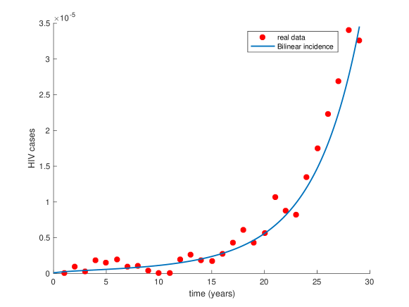
In Figure 2, we observe that model (1) fits the real data reported in [26]. The HIV cases described by model (1) are given by $I(t)+C(t)+\mu\left(I(t)+C(t)\right)$ for $t\in[0,29]$, which corresponds to the interval of time between the years of 1986 ($t=0$) and 2015 ($t=29$).

Figure 2: Model (1) fitting the data of HIV cases in Morocco between 1986 ($t=0$) and 2015 ($t=29$).

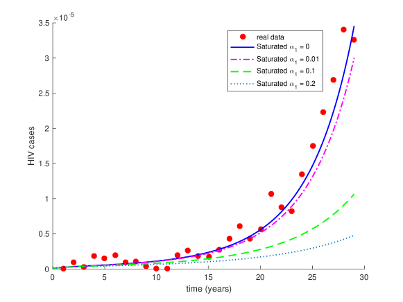
For the saturated incidence function $\dfrac{\beta S}{1+\alpha_{1}S}$ [19], see Figure 3.

Figure 3: Saturated incidence function $\dfrac{\beta S}{1+\alpha_{1}S}$ with $\alpha_{1}\in\{0,0.01,0.1,0.2\}$. Time $t=0$ corresponds to the year 1986.

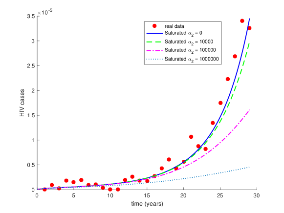
For the saturated incidence function $\dfrac{\beta S}{1+\alpha_{2}I}$ [39], see Figure 4.

Figure 4: Saturated incidence function $\dfrac{\beta S}{1+\alpha_{2}I}$ with $\alpha_{2}\in\{0,10^{4},10^{5},10^{6}\}$. Time $t=0$ corresponds to the year 1986.

For the Beddington–DeAngelis incidence function $\dfrac{\beta S}{1+\alpha_{1}S+\alpha_{2}I}$ [1, 3, 7], see Figure 5.

Figure 5: Beddington–DeAngelis incidence function $\dfrac{\beta S}{1+\alpha_{1}S+\alpha_{2}I}$ with $\alpha_{1}\in\{0,0.01,0.1\}$ and $\alpha_{2}\in\{0,10^{4},10^{5},10^{6}\}$. Time $t=0$ corresponds to the year 1986.

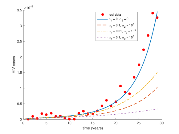
For the specific non-linear incidence function $\dfrac{\beta S}{1+\alpha_{1}S+\alpha_{2}I+\alpha_{3}SI}$ [10, 11, 14, 21, 25], see Figure 6.

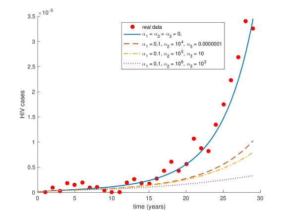
Figure 6: Specific non-linear incidence function $\dfrac{\beta S}{1+\alpha_{1}S+\alpha_{2}I+\alpha_{3}SI}$ with $\alpha_{1}\in\{0,0.1\}$, $\alpha_{2}\in\{0,10^{4},10^{5},10^{6}\}$ and $\alpha_{3}\in\{0,10^{-6},10,10^{2}\}$. Time $t=0$ corresponds to the year 1986.

In Tables 3 and 4, we compute the basic reproduction number $R_{0}$ for each incidence function proposed in Table 1 with the parameter values from Table 2.

Table 3: Basic reproduction number for some special incidence functions.

Incidence functions	${f(S,I)}$	$R_{0}$
Bilinear	$\beta S$	$7.5340$
Saturated I	$\dfrac{\beta S}{1+\alpha_{1}S}$	$\dfrac{0.0031}{0.0009\,\alpha_{1}+0.0004}$
Saturated II	$\dfrac{\beta S}{1+\alpha_{2}I}$	$7.5340$
Beddington–DeAngelis	$\dfrac{\beta S}{1+\alpha_{1}S+\alpha_{2}I}$	$\dfrac{0.0031}{0.0009\,\alpha_{1}+0.0004}$
Crowley–Martin	$\dfrac{\beta S}{1+\alpha_{1}S+\alpha_{2}I+\alpha_{1}\alpha_{2}SI}$	$\dfrac{0.0031}{0.0009\,\alpha_{1}+0.0004}$
Specific non-linear	$\dfrac{\beta S}{1+\alpha_{1}S+\alpha_{2}I+\alpha_{3}SI}$	$\dfrac{0.0031}{0.0009\,\alpha_{1}+0.0004}$
Hattaf–Yousfi	$\dfrac{\beta S}{\alpha_{0}+\alpha_{1}S+\alpha_{2}I+\alpha_{3}SI}$	$\dfrac{0.0031}{0.0004\,\alpha_{0}+0.0009\,\alpha_{1}}$

Table 4: Basic reproduction number for different values of $\alpha_{1}$ for the incidence function Saturated I, Beddington–DeAngelis, Crowley–Martin and Specific non-linear.

$\alpha_{1}$	$0.01$	$0.1$	$0.2$
$R_{0}$	$7.3725$	$6.1804$	$5.2392$

In Table 5, we present the sensitivity index of parameters $\beta$, $\phi$, $\rho$, $\alpha$ and $\omega$, computed for the parameter values given in Table 2.

Table 5: Sensitivity index of $R_{0}$ for parameter values given in Table 2 for the bilinear incidence function $f(S,I)=\beta S$.

Parameter	Sensitivity index
$\beta$	+1
$\phi$	$-0.5947$
$\rho$	$-0.3437$
$\alpha$	$+0.0844$
$\omega$	$+0.5170$

6 Conclusion

In this paper we considered a varying population size in a homogeneously mixed population described by a non-linear mathematical model for HIV/AIDS transmission. We have studied the global dynamics of the model with a general incidence function. This general incidence function depends on the susceptible and HIV-infected individuals with no AIDS symptoms, which are not under ART treatment and therefore transmit the HIV virus. We have shown that the model can describe very well the reality given by the data of HIV/AIDS infection in Morocco from 1986 to 2015, when the incidence function is carefully chosen. The sensitivity index results of the basic reproduction number $R_{0}$ with respect to the parameters show that the effective contact rate $\beta$ is the most sensitive parameter, that is, a small perturbation in the effective contact rate value leads to relevant quantitative changes, since an increase (decrease) of $\beta$ by a given percentage increases (decreases) $R_{0}$ by that same percentage. For this reason, the estimation of $\beta$ should be carefully done and targeted by intervention strategies to engage the UNAIDS worldwide goal of ending the AIDS epidemic by 2030.

References

• [1] J. R. Beddington, Mutual interference between parasites or predators and its effect on searching efficiency, J. Animal Ecol 44 (1975), 331–341.
• [2] C. P. Bhunu, W. Garira and Z. Mukandavire, Modeling HIV/AIDS and tuberculosis coinfection, Bull. Math. Biol. 71 (2009), no. 7, 1745–1780.
• [3] R. S. Cantrell and C. Cosner, On the dynamics of predator-prey models with the Beddington-DeAngelis functional response, J. Math. Anal. Appl. 257 (2001), no. 1, 206–222.
• [4] V. Capasso and G. Serio, A generalization of the Kermack-McKendrick deterministic epidemic model, Math. Biosci. 42 (1978), no. 1-2, 43–61.
• [5] N. Chitnis, J. M. Hyman and J. M. Cushing, Determining important parameters in the spread of malaria through the sensitivity analysis of a mathematical model, Bull. Math. Biol. 70 (2008), no. 5, 1272–1296.
• [6] P. H. Crowley and E. K. Martin, Functional responses and interference within and between year classes of a dragonfly population, J. North. Am. Benth. Soc. 8 (1989), 211–221.
• [7] D. L. DeAngelis, R. A. Goldstein and R. V. O’Neill, A model for tropic interaction, Ecology 56 (1975), no. 4, 881–892.
• [8] J. Djordjevic, C. J. Silva and D. F. M. Torres, A stochastic SICA epidemic model for HIV transmission, Appl. Math. Lett. 84 (2018), 168–175. arXiv:1805.01425
• [9] K. Hattaf, A. A. Lashari, Y. Louartassi and N. Yousfi, A delayed SIR epidemic model with general incidence rate, Electron. J. Qual. Theory Differ. Equ. 2013 (2013), no. 3, 9 pp.
• [10] K. Hattaf, M. Mahrouf, J. Adnani and N. Yousfi, Qualitative analysis of a stochastic epidemic model with specific functional response and temporary immunity, Phys. A 490 (2018), 591–600.
• [11] K. Hattaf and N. Yousfi, Global dynamics of a delay reaction-diffusion model for viral infection with specific functional response, Comput. Appl. Math. 34 (2015), no. 3, 807–818.
• [12] K. Hattaf and N. Yousfi, A class of delayed viral infection models with general incidence rate and adaptive immune response, Int. J. Dyn. Control 4 (2016), no. 3, 254–265.
• [13] K. Hattaf, N. Yousfi and A. Tridane, Mathematical analysis of a virus dynamics model with general incidence rate and cure rate, Nonlinear Anal. Real World Appl. 13 (2012), no. 4, 1866–1872.
• [14] K. Hattaf, N. Yousfi and A. Tridane, Stability analysis of a virus dynamics model with general incidence rate and two delays, Appl. Math. Comput. 221 (2013), 514–521.
• [15] K. Hattaf, N. Yousfi and A. Tridane, A delay virus dynamics model with general incidence rate, Differ. Equ. Dyn. Syst. 22 (2014), no. 2, 181–190.
• [16] C. Ji and D. Jiang, Threshold behaviour of a stochastic SIR model, Appl. Math. Model. 38 (2014), no. 21-22, 5067–5079.
• [17] W. O. Kermack and A. G. McKendrick, Contributions to the mathematical theory of epidemics, part I, Proc. Roy. Soc. Edinburgh A 115 (1927), 700–721.
• [18] J. P. LaSalle, The stability of dynamical systems, Society for Industrial and Applied Mathematics, Philadelphia, PA, 1976.
• [19] X. Liu and L. Yang, Stability analysis of an SEIQV epidemic model with saturated incidence rate, Nonlinear Anal. Real World Appl. 13 (2012), no. 6, 2671–2679.
• [20] X.-Q. Liu, S.-M. Zhong, B.-D. Tian and F.-X. Zheng, Asymptotic properties of a stochastic predator-prey model with Crowley-Martin functional response, J. Appl. Math. Comput. 43 (2013), no. 1-2, 479–490.
• [21] E. M. Lotfi, M. Maziane, K. Hattaf and N. Yousfi, Partial differential equations of an epidemic model with spatial diffusion, Int. J. Partial Differ. Equ. 2014 (2014), Art. ID 186437, 6 pp.
• [22] E. M. Lotfi, M. Maziane, M. Mahrouf, K. Hattaf and N. Yousfi, Global stability of a diffused SIR epidemic model with general incidence rate and time delay, Int. J. Math. Anal. (Ruse) 10 (2016), no. 17, 807–816.
• [23] M. Mahrouf, K. Hattaf and N. Yousfi, Dynamics of a stochastic viral infection model with immune response, Math. Model. Nat. Phenom. 12 (2017), no. 5, 15–32.
• [24] J. P. Mateus, P. Rebelo, S. Rosa, C. M. Silva and D. F. M. Torres, Optimal control of non-autonomous SEIRS models with vaccination and treatment, Discrete Contin. Dyn. Syst. Ser. S 11 (2018), no. 6, 1179–1199. arXiv:1706.06843
• [25] M. Maziane, E. M. Lotfi, K. Hattaf and N. Yousfi, Dynamics of a class of HIV infection models with cure of infected cells in eclipse stage, Acta Biotheoretica 63 (2015), no. 4, 363–380.
• [26] Ministry of Health, Morocco, Department of Epidemiology and Disease Control, http://www.sante.gov.ma/Pages/Accueil.aspx
• [27] A. S. Perelson, P. Essunger, Y. Cao, M. Vesanen, A. Hurley, K. Saksela, M. Markowitz and D. D. Ho, Decay characteristics of HIV-1-infected compartments during combination therapy, Nature 387 (1997), 188–191.
• [28] Population Data, http://www.populationdata.net
• [29] Population Data, Maroc, http://www.populationdata.net/pays/maroc
• [30] H. S. Rodrigues, M. T. T. Monteiro and D. F. M. Torres, Sensitivity analysis in a dengue epidemiological model, Conf. Papers in Math. 2013 (2013), Art. ID 721406, 7 pp. arXiv:1307.0202
• [31] O. Sharomi, C. N. Podder, A. B. Gumel and B. Song, Mathematical analysis of the transmission dynamics of HIV/TB coinfection in the presence of treatment, Math. Biosci. Eng. 5 (2008), no. 1, 145–174.
• [32] C. J. Silva and D. F. M. Torres, A TB-HIV/AIDS coinfection model and optimal control treatment, Discrete Contin. Dyn. Syst. 35 (2015), no. 9, 4639–4663. arXiv:1501.03322
• [33] C. J. Silva and D. F. M. Torres, A SICA compartmental model in epidemiology with application to HIV/AIDS in Cape Verde, Ecological Complexity 30 (2017), 70–75. arXiv:1612.00732
• [34] UNAIDS, http://www.unaids.org
• [35] UNAIDS, Fast-Track – Ending the AIDS epidemic by 2030, 2014. http://www.unaids.org/sites/default/files/media_asset/JC2686_WAD2014report_en.pdf
• [36] P. van den Driessche and J. Watmough, Reproduction numbers and sub-threshold endemic equilibria for compartmental models of disease transmission, Math. Biosci. 180 (2002), 29–48.
• [37] J.-J. Wang, J.-Z. Zhang and Z. Jin, Analysis of an SIR model with bilinear incidence rate, Nonlinear Anal. Real World Appl. 11 (2010), no. 4, 2390–2402.
• [38] World Bank Data, Morocco, http://data.worldbank.org/country/morocco
• [39] Y. Zhao and D. Jiang, The threshold of a stochastic SIRS epidemic model with saturated incidence, Appl. Math. Lett. 34 (2014), 90–93.
• [40] X. Zhou and J. Cui, Global stability of the viral dynamics with Crowley-Martin functional response, Bull. Korean Math. Soc. 48 (2011), no. 3, 555–574.
• [41] M. Zwahlen and M. Egger, Progression and mortality of untreated HIV-positive individuals living in resource-limited settings: update of literature review and evidence synthesis, Report on UNAIDS obligation no HQ/05/422204, Bern, 2006.