\vol\fpage\lpage

Domain Adaptation on Graphs by Learning Graph Topologies: Theoretical Analysis and an Algorithm

Elif Vural1 
1
Department of Electrical and Electronics Engineering
velif@metu.edu.tr. This work has been supported by the TÜBİTAK 2232 program, project no. 117C007.
   Middle East Technical University    Ankara    Turkey

Abstract

Traditional machine learning algorithms assume that the training and test data have the same distribution, while this assumption does not necessarily hold in real applications. Domain adaptation methods take into account the deviations in the data distribution. In this work, we study the problem of domain adaptation on graphs. We consider a source graph and a target graph constructed with samples drawn from data manifolds. We study the problem of estimating the unknown class labels on the target graph using the label information on the source graph and the similarity between the two graphs. We particularly focus on a setting where the target label function is learnt such that its spectrum is similar to that of the source label function. We first propose a theoretical analysis of domain adaptation on graphs and present performance bounds that characterize the target classification error in terms of the properties of the graphs and the data manifolds. We show that the classification performance improves as the topologies of the graphs get more balanced, i.e., as the numbers of neighbors of different graph nodes become more proportionate, and weak edges with small weights are avoided. Our results also suggest that graph edges between too distant data samples should be avoided for good generalization performance. We then propose a graph domain adaptation algorithm inspired by our theoretical findings, which estimates the label functions while learning the source and target graph topologies at the same time. The joint graph learning and label estimation problem is formulated through an objective function relying on our performance bounds, which is minimized with an alternating optimization scheme. Experiments on synthetic and real data sets suggest that the proposed method outperforms baseline approaches.

keywords:
Domain adaptation, data classification, graph Fourier basis, graph Laplacian, performance bounds.

1 Introduction

Classical machine learning methods are based on the assumption that the training data and the test data have the same distribution. A classifier is learnt on the training data, which is then used to estimate the unknown class labels of the test data. On the other hand, domain adaptation methods consider a setting where the distribution of the test data is different from that of the training data [1, 2, 3, 4]. Given many labeled samples in a source domain and much fewer labeled samples in a target domain, domain adaptation algorithms exploit the information available in both domains in order to improve the performance of classification in the target domain. Meanwhile, many machine learning applications nowadays involve inference problems on graph domains such as social networks and communication networks. Moreover, in most problems data samples conform to a low-dimensional manifold model; for instance, face images of a person captured from different camera angles lie on a low-dimensional manifold. In such problems, graphs models are widely used as they are very convenient for approximating the actual data manifolds. Hence, domain adaptation on graphs arises as an important problem of interest, which we study in this work. We first present performance bounds for transferring the knowledge of class labels between a pair of graphs. We then use these bounds to develop an algorithm that computes the structures of the source and the target graphs and estimates the unknown class labels at the same time.

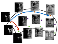
Many graph-based learning methods rely on the assumption that the label function varies slowly on the data graph. However, this assumption does not always hold as shown in Figure 1. A face manifold is illustrated in Figure 1, each point of which corresponds to a face image that belongs to one of three different subjects. In this example, the class label function varies slowly along the blue direction, where images belong to the same subject. On the other hand, along the red direction the face images of different subjects get too close to each other due to extreme illumination conditions. Hence, the label function has fast variation along the red direction on the manifold.

Although it is common to assume that the label function varies slowly in problems concerning a single graph, in a problem with more than one graph it is possible to learn the speed of variation of the label function and share this information across different graphs. This is illustrated in Figure 1, where the characteristics of the variation of the label function can be learnt on a source graph where many class labels are available. Then, the purpose of graph domain adaptation is to transfer this information to a target graph that contains very few labels and estimate the unknown class labels. We studied this problem in our previous work [5], where we proposed a method called Spectral Domain Adaptation (SDA).
Refer to caption
Refer to caption
Figure 1: (a) Illustration of a face manifold where the label function varies at different speeds along different directions (b) Illustration of domain adaptation on graphs

In order to optimize the performance of graph domain adaptation methods, it is important to theoretically characterize their performance limits. The classification performance significantly depends on the structures of the source and the target graphs and the similarity between them. In particular, in problems where the graphs are constructed from data samples coming from data manifolds, the properties of the graphs such as the locations and the weights of the edges, and the number of neighbors of graph nodes largely influence the performance of learning. A thorough characterization of the effects of such parameters in conjunction with the geometry of the data manifolds is necessary to understand the performance limits of graph domain adaptation.

Our contribution in this study is twofold. We first propose a theoretical study of domain adaptation on graphs. We consider a source graph and a target graph constructed with data samples coming respectively from a source manifold and a target manifold. We theoretically analyze the performance of classification on the target graph. In particular, we focus on the estimation error of the target label function and analyze how this error varies with the graph properties, the sampling density of data, and the geometric properties of the data manifolds. Our theoretical analysis suggests that very sparse graphs with too few edges and very dense graphs with too many edges should be avoided, as well as too small edge weights. The smoothness of the label function is shown to positively influence the performance of learning. We show that, under certain assumptions, the estimation error of the target label function decreases with the sampling density of the manifolds at a rate of O(N1/d)𝑂superscript𝑁1𝑑O(N^{-1/d}), where N𝑁N is the number of samples and d𝑑d is the intrinsic dimension of the manifolds. Next, we use these theoretical findings to propose a graph domain adaptation algorithm that jointly estimates the class labels of the source and the target data and the topologies of the source and the target graphs. In particular, we optimize the source and the target graph weight matrices, which fully determine the graph topologies, in order to properly control parameters such as the number of neighbors, the minimum edge weights, and the smoothness of the label functions on the graphs. Experimental results on synthetic and real data sets show that the proposed method with learnt graph topologies outperforms reference domain adaptation methods with fixed graph topologies and other baseline algorithms.

The rest of the paper is organized as follows. In Section 2, we briefly overview the related literature. In Section 3, we first overview frequency analysis on graphs and then present theoretical bounds for graph domain adaptation. In Section 4, we present a graph domain adaptation algorithm that is motivated by our theoretical findings. We experimentally evaluate the proposed method in Section 5 and conclude in Section 6.

2 Related Work

We first overview some common approaches in domain adaptation. In several previous works the covariate shift problem is studied, where the two distributions are matched with reweighting [6, 7]. The studies in [8, 9] propose to train a common classifier after mapping the data to a higher dimensional domain via feature augmentation. Another common approach is to align or match the two domains by mapping them to a common domain with projections or transformations [10, 11, 12, 13, 14, 15, 16, 17].

Several domain adaptation methods model data with a graph and make use of the assumption that the label function varies smoothly on the graph [3, 18, 19]. The unsupervised method in [20] formulates the domain adaptation problem as a graph matching problem. The algorithms in [21] and [22] aim to compute a pair of bases on the source graph and the target graph that approximate the Fourier bases and jointly diagonalize the two graph Laplacians. These methods are applied to problems such as clustering and 3D shape analysis. Our recent work [5] also relies on representations with graph Fourier bases, however, in the context of domain adaptation. Our study in this paper provides insights for such graph-based methods involving the notion of smoothness on graphs and representations in graph bases.

The problem of learning graph topologies from data has drawn particular interest in the recent years. Various efforts have focused on the inference of the graph topology from a set of training signals that are known to vary smoothly on the graph [23, 24, 25]. However, such approaches differ from ours in that they address an unsupervised learning problem. Our method, on the other hand, actively incorporates the information of the class labels when learning the graph structures in a domain adaptation framework. In some earlier studies, graph structures have been learnt in a semi-supervised setting [26, 27]. However, unlike as in our work, the graph Laplacians are restricted to a linear combination of a prescribed set of kernels in these methods.

Some previous studies analyzing the domain adaptation problem from a theoretical perspective are the following. Performance bounds for importance reweighting have been proposed in [6] and [28]. The studies in [29, 30, 31, 32, 33] bound the target loss in terms of the deviation between the source distribution and the target distribution. While such studies present a theoretical analysis of domain adaptation, none of them treat the domain adaptation problem in a graph setting. To the best of our knowledge, our theoretical analysis is the first to focus particularly on the graph domain adaptation problem.

3 Theoretical Analysis of Graph Domain Adaptation

3.1 Overview of Signal Processing on Graphs

We first briefly overview some basic concepts regarding spectral graph theory and signal processing on graphs [34, 35]. Let G=(V,E)𝐺𝑉𝐸G=(V,E) be a graph consisting of N𝑁N vertices denoted by V={xi}i=1N𝑉superscriptsubscriptsubscript𝑥𝑖𝑖1𝑁V=\{x_{i}\}_{i=1}^{N} and edges E𝐸E. The N×N𝑁𝑁N\times N symmetric matrix W𝑊W consisting of nonnegative edge weights is called the weight matrix, where Wijsubscript𝑊𝑖𝑗W_{ij} is the weight of the edge between the nodes xisubscript𝑥𝑖x_{i} and xjsubscript𝑥𝑗x_{j}. If there is no edge between xisubscript𝑥𝑖x_{i} and xjsubscript𝑥𝑗x_{j}, then Wij=0subscript𝑊𝑖𝑗0W_{ij}=0. The degree di=j=1NWijsubscript𝑑𝑖superscriptsubscript𝑗1𝑁subscript𝑊𝑖𝑗d_{i}=\sum_{j=1}^{N}W_{ij} of a vertex xisubscript𝑥𝑖x_{i} is defined as the total weight of the edges linked to it. The diagonal matrix D𝐷D with entries given by Dii=disubscript𝐷𝑖𝑖subscript𝑑𝑖D_{ii}=d_{i} is called the degree matrix.

A graph signal f:V:𝑓𝑉f:V\rightarrow\mathbb{R} is a function that takes a real value on each vertex. A signal f𝑓f on a graph with N𝑁N vertices can then be regarded as an N𝑁N-dimensional vector f=[f(x1)f(xN)]TN.𝑓superscriptdelimited-[]𝑓subscript𝑥1𝑓subscript𝑥𝑁𝑇superscript𝑁f=[f(x_{1})\dots f(x_{N})]^{T}\in\mathbb{R}^{N}. The graph Laplacian matrix defined as L=DW𝐿𝐷𝑊L=D-W is of special importance in spectral graph theory [34, 35]. L𝐿L can be seen as an operator acting on the function f𝑓f through the matrix multiplication Lf𝐿𝑓Lf, and it has been shown to be the graph equivalent of the Laplace operator in Euclidean domains, or the Laplace-Beltrami operator on manifold domains [34, 36, 37]. Recalling that the complex exponentials fundamental in classical signal processing have the special property that they are the eigenfunctions of the Laplace operator, one can extend the notion of frequency to graph domains. Relying on the analogy between the Laplace operator and the graph Laplacian L𝐿L, one can define a Fourier basis on graphs, which consists of the eigenvectors of L𝐿L.

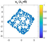
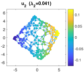
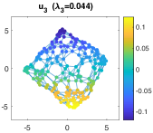
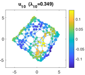
Let u1,,uNsubscript𝑢1subscript𝑢𝑁u_{1},\dots,u_{N} denote the eigenvectors of the graph Laplacian, where Luk=λkuk𝐿subscript𝑢𝑘subscript𝜆𝑘subscript𝑢𝑘Lu_{k}=\lambda_{k}u_{k} for k=1,,N𝑘1𝑁k=1,\dots,N. Here, each uksubscript𝑢𝑘u_{k} is a graph Fourier basis vector of frequency λksubscript𝜆𝑘\lambda_{k}. The eigenvector u1subscript𝑢1u_{1} with the smallest eigenvalue λ1=0subscript𝜆10\lambda_{1}=0 is always a constant function on the graph, and the speed of variation of uksubscript𝑢𝑘u_{k} on the graph increases for increasing k𝑘k. The eigenvalues λ1,,λNsubscript𝜆1subscript𝜆𝑁\lambda_{1},\dots,\lambda_{N} of the graph Laplacian correspond to frequencies such that λksubscript𝜆𝑘\lambda_{k} provides a measure of the speed of variation of the signal uksubscript𝑢𝑘u_{k} on the graph. The Fourier basis vectors of an example graph are illustrated in Figure 2. In particular, the speed of variation of a signal f𝑓f over the graph is

fTLf=12i,j=1NWij(f(xi)f(xj))2,superscript𝑓𝑇𝐿𝑓12superscriptsubscript𝑖𝑗1𝑁subscript𝑊𝑖𝑗superscript𝑓subscript𝑥𝑖𝑓subscript𝑥𝑗2f^{T}Lf=\frac{1}{2}\sum_{i,j=1}^{N}W_{ij}(f(x_{i})-f(x_{j}))^{2},

which takes larger values if the function f𝑓f varies more abruptly between neighboring graph vertices. Notice that the above term becomes the corresponding eigenvalue λksubscript𝜆𝑘\lambda_{k} of L𝐿L when f𝑓f is taken as uksubscript𝑢𝑘u_{k}, since ukTLuk=λk.superscriptsubscript𝑢𝑘𝑇𝐿subscript𝑢𝑘subscript𝜆𝑘u_{k}^{T}Lu_{k}=\lambda_{k}.

Refer to caption
Refer to caption
Refer to caption
Refer to caption
Refer to caption
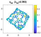
Figure 2: Fourier basis vectors of an example graph. The eigenvectors u1subscript𝑢1u_{1}, u2subscript𝑢2u_{2}, u3subscript𝑢3u_{3}, u10subscript𝑢10u_{10}, u50subscript𝑢50u_{50} of the graph Laplacian are plotted as graph signals in panels (a)-(e), where yellow and blue colors respectively indicate positive and negative values. The first Fourier basis vector u1subscript𝑢1u_{1} has constant amplitude as its frequency is λ1=0subscript𝜆10\lambda_{1}=0. The signals u2subscript𝑢2u_{2} and u3subscript𝑢3u_{3} have small frequencies around 0.040.040.04 and they slowly oscillate along different directions on the graph. The signal u10subscript𝑢10u_{10} has a larger frequency λ10=0.349subscript𝜆100.349\lambda_{10}=0.349, hence its speed of oscillation is higher. Among the five signals, u50subscript𝑢50u_{50} has the highest frequency λ50=2.382subscript𝜆502.382\lambda_{50}=2.382 and it has the fastest variation on the graph.

This definition of the graph Fourier basis allows the extension of the Fourier transform to graph domains as follows. Let U=[u1u2uN]N×N𝑈delimited-[]subscript𝑢1subscript𝑢2subscript𝑢𝑁superscript𝑁𝑁U=[u_{1}u_{2}\dots u_{N}]\in\mathbb{R}^{N\times N} be the matrix consisting of the graph Fourier basis vectors. Then, for a graph signal fN𝑓superscript𝑁f\in\mathbb{R}^{N}, the Fourier transform of f𝑓f can simply be computed as α=UTf,𝛼superscript𝑈𝑇𝑓\alpha=U^{T}f, where α=[α1αN]T𝛼superscriptdelimited-[]subscript𝛼1subscript𝛼𝑁𝑇\alpha=[\alpha_{1}\dots\alpha_{N}]^{T} is the vector consisting of the Fourier coefficients. Here αk=ukTfsubscript𝛼𝑘superscriptsubscript𝑢𝑘𝑇𝑓\alpha_{k}=u_{k}^{T}f is the k𝑘k-th Fourier coefficient given by the inner product of f𝑓f and the Fourier basis vector uksubscript𝑢𝑘u_{k}. Note that the graph Fourier basis U𝑈U is orthonormal as in classical signal processing; hence, the signal f𝑓f can be reconstructed from its Fourier coefficients as f=Uα𝑓𝑈𝛼f=U\alpha.

3.2 Notation and Setting

We now discuss the problem of domain adaptation on graphs and set the notation used in this paper. We consider a source graph Gs=(Vs,Es)superscript𝐺𝑠superscript𝑉𝑠superscript𝐸𝑠G^{s}=(V^{s},E^{s}) with vertices Vs={xis}i=1Nssuperscript𝑉𝑠superscriptsubscriptsubscriptsuperscript𝑥𝑠𝑖𝑖1subscript𝑁𝑠V^{s}=\{x^{s}_{i}\}_{i=1}^{N_{s}} and edges Essuperscript𝐸𝑠E^{s}; and a target graph Gt=(Vt,Et)superscript𝐺𝑡superscript𝑉𝑡superscript𝐸𝑡G^{t}=(V^{t},E^{t}) with vertices Vt={xit}i=1Ntsuperscript𝑉𝑡superscriptsubscriptsubscriptsuperscript𝑥𝑡𝑖𝑖1subscript𝑁𝑡V^{t}=\{x^{t}_{i}\}_{i=1}^{N_{t}} and edges Etsuperscript𝐸𝑡E^{t}. Let Wssuperscript𝑊𝑠W^{s} and Wtsuperscript𝑊𝑡W^{t} denote the weight matrices, and let Lssuperscript𝐿𝑠L^{s} and Ltsuperscript𝐿𝑡L^{t} be the Laplacians of the source and the target graphs. Let fssuperscript𝑓𝑠f^{s} and ftsuperscript𝑓𝑡f^{t} be the label functions on the source and the target graphs, which represent class labels in a classification problem and continuously varying entities in a regression problem. We assume that some class labels are known as yis=fs(xis)subscriptsuperscript𝑦𝑠𝑖superscript𝑓𝑠subscriptsuperscript𝑥𝑠𝑖y^{s}_{i}=f^{s}(x^{s}_{i}) for iILs{1,,Ns}𝑖superscriptsubscript𝐼𝐿𝑠1subscript𝑁𝑠i\in I_{L}^{s}\subset\{1,\dots,N_{s}\}, and yit=ft(xit)subscriptsuperscript𝑦𝑡𝑖superscript𝑓𝑡subscriptsuperscript𝑥𝑡𝑖y^{t}_{i}=f^{t}(x^{t}_{i}) for iILt{1,,Nt}𝑖superscriptsubscript𝐼𝐿𝑡1subscript𝑁𝑡i\in I_{L}^{t}\subset\{1,\dots,N_{t}\}, where ILssuperscriptsubscript𝐼𝐿𝑠I_{L}^{s} and ILtsuperscriptsubscript𝐼𝐿𝑡I_{L}^{t} are index sets. Many samples are labeled in the source domain and few samples are labeled in the target domain, i.e., |ILt||ILs|much-less-thansuperscriptsubscript𝐼𝐿𝑡superscriptsubscript𝐼𝐿𝑠|I_{L}^{t}|\ll|I_{L}^{s}|. Given the available labels {yis}iILssubscriptsubscriptsuperscript𝑦𝑠𝑖𝑖superscriptsubscript𝐼𝐿𝑠\{y^{s}_{i}\}_{i\in I_{L}^{s}} and {yit}iILtsubscriptsubscriptsuperscript𝑦𝑡𝑖𝑖superscriptsubscript𝐼𝐿𝑡\{y^{t}_{i}\}_{i\in I_{L}^{t}}, the purpose of graph domain adaptation is to compute accurate estimates f^ssuperscript^𝑓𝑠\hat{f}^{s}, f^tsuperscript^𝑓𝑡\hat{f}^{t} of fssuperscript𝑓𝑠f^{s} and ftsuperscript𝑓𝑡f^{t}.

All domain adaptation methods rely on a certain relationship between the source and the target domains. In this study, we consider a setting where a relationship can be established between the source and the target graphs through the frequency content of the label functions. Let fs=Usαssuperscript𝑓𝑠superscript𝑈𝑠superscript𝛼𝑠f^{s}=U^{s}\alpha^{s} and ft=Utαtsuperscript𝑓𝑡superscript𝑈𝑡superscript𝛼𝑡f^{t}=U^{t}\alpha^{t} denote the decompositions of the label functions over the source Fourier basis Us=[u1suNss]Ns×Nssuperscript𝑈𝑠delimited-[]superscriptsubscript𝑢1𝑠superscriptsubscript𝑢subscript𝑁𝑠𝑠superscriptsubscript𝑁𝑠subscript𝑁𝑠U^{s}=[u_{1}^{s}\dots u_{N_{s}}^{s}]\in\mathbb{R}^{N_{s}\times N_{s}} and the target Fourier basis Ut=[u1tuNtt]Nt×Ntsuperscript𝑈𝑡delimited-[]superscriptsubscript𝑢1𝑡superscriptsubscript𝑢subscript𝑁𝑡𝑡superscriptsubscript𝑁𝑡subscript𝑁𝑡U^{t}=[u_{1}^{t}\dots u_{N_{t}}^{t}]\in\mathbb{R}^{N_{t}\times N_{t}}. We assume a setting where the source and the target label functions have similar spectra, hence, similar Fourier coefficients.

We have observed in our previous work [5] that, when computing the estimates f^ssuperscript^𝑓𝑠\hat{f}^{s} and f^tsuperscript^𝑓𝑡\hat{f}^{t} of the label functions, it is useful to represent them in the reduced bases U¯sNs×Rsuperscript¯𝑈𝑠superscriptsubscript𝑁𝑠𝑅\overline{U}^{s}\in\mathbb{R}^{N_{s}\times R} and U¯tNt×Rsuperscript¯𝑈𝑡superscriptsubscript𝑁𝑡𝑅\overline{U}^{t}\in\mathbb{R}^{N_{t}\times R}, which consist of the first R𝑅R Fourier basis vectors of smallest frequencies. This not only reduces the complexity of the problem but also has a regularization effect since components of very high frequency are excluded from the estimates. The estimates of fssuperscript𝑓𝑠f^{s} and ftsuperscript𝑓𝑡f^{t} are then obtained in the form f^s=U¯sα¯ssuperscript^𝑓𝑠superscript¯𝑈𝑠superscript¯𝛼𝑠\hat{f}^{s}=\overline{U}^{s}\overline{\alpha}^{s} and f^t=U¯tα¯t,superscript^𝑓𝑡superscript¯𝑈𝑡superscript¯𝛼𝑡\hat{f}^{t}=\overline{U}^{t}\overline{\alpha}^{t}, where α¯sRsuperscript¯𝛼𝑠superscript𝑅\overline{\alpha}^{s}\in\mathbb{R}^{R} and α¯tRsuperscript¯𝛼𝑡superscript𝑅\overline{\alpha}^{t}\in\mathbb{R}^{R} are reduced Fourier coefficient vectors. In [5], the label functions are estimated such that their Fourier coefficients α¯ssuperscript¯𝛼𝑠\overline{\alpha}^{s} and α¯tsuperscript¯𝛼𝑡\overline{\alpha}^{t} are close to each other and the estimates f^ssuperscript^𝑓𝑠\hat{f}^{s} and f^tsuperscript^𝑓𝑡\hat{f}^{t} are consistent with the available labels.

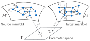
In our theoretical analysis of graph domain adaptation, we consider a setting where graphs nodes are sampled from data manifolds. Let {xis}i=1Nsssuperscriptsubscriptsubscriptsuperscript𝑥𝑠𝑖𝑖1subscript𝑁𝑠superscript𝑠\{x^{s}_{i}\}_{i=1}^{N_{s}}\subset\mathcal{M}^{s} and {xit}i=1Nttsuperscriptsubscriptsubscriptsuperscript𝑥𝑡𝑖𝑖1subscript𝑁𝑡superscript𝑡\{x^{t}_{i}\}_{i=1}^{N_{t}}\subset\mathcal{M}^{t} denote source and target graph nodes sampled from a source data manifold ssuperscript𝑠\mathcal{M}^{s} and a target data manifold tsuperscript𝑡\mathcal{M}^{t}. We assume that the source and the target data manifolds are generated through a pair of functions gs:Γs:superscript𝑔𝑠Γsuperscript𝑠g^{s}:\Gamma\rightarrow\mathcal{M}^{s} and gt:Γt:superscript𝑔𝑡Γsuperscript𝑡g^{t}:\Gamma\rightarrow\mathcal{M}^{t} defined on a common parameter space ΓΓ\Gamma. Then, each manifold sample can be expressed as xis=gs(γis)subscriptsuperscript𝑥𝑠𝑖superscript𝑔𝑠subscriptsuperscript𝛾𝑠𝑖x^{s}_{i}=g^{s}(\gamma^{s}_{i}) and xit=gt(γit),subscriptsuperscript𝑥𝑡𝑖superscript𝑔𝑡subscriptsuperscript𝛾𝑡𝑖x^{t}_{i}=g^{t}(\gamma^{t}_{i}), where γisΓsubscriptsuperscript𝛾𝑠𝑖Γ\gamma^{s}_{i}\in\Gamma and γitΓsubscriptsuperscript𝛾𝑡𝑖Γ\gamma^{t}_{i}\in\Gamma are parameter vectors as illustrated in Figure 3. The parameter vectors are assumed to capture the source of variation generating the data manifolds. For instance, in a face recognition problem, γissubscriptsuperscript𝛾𝑠𝑖\gamma^{s}_{i} and γitsubscriptsuperscript𝛾𝑡𝑖\gamma^{t}_{i} may represent rotation angles of the cameras viewing the subjects; and the discrepancy between ssuperscript𝑠\mathcal{M}^{s} and tsuperscript𝑡\mathcal{M}^{t} may result from the change in the illumination conditions. Note that in domain adaptation no relation is assumed to be known between γissubscriptsuperscript𝛾𝑠𝑖\gamma^{s}_{i} and γitsubscriptsuperscript𝛾𝑡𝑖\gamma^{t}_{i}. Moreover, the parameters {γis}subscriptsuperscript𝛾𝑠𝑖\{\gamma^{s}_{i}\}, {γit}subscriptsuperscript𝛾𝑡𝑖\{\gamma^{t}_{i}\} and the functions gssuperscript𝑔𝑠g^{s}, gtsuperscript𝑔𝑡g^{t} are often not known in practice. Although we consider this setting in our theoretical analysis, the practical algorithm we propose in Section 4 will not require the knowledge of these parameters.
Refer to caption


Figure 3: Illustration of the domain adaptation setting considered in our study

3.3 Performance Bounds for Graph Domain Adaptation

In this section, we analyze the error between the estimated target label function f^tsuperscript^𝑓𝑡\hat{f}^{t} and the true target label function ftsuperscript𝑓𝑡f^{t}. We would like to derive an upper bound for the estimation error

E=f^tft2=i=1Nt(f^t(xit)ft(xit))2=i=1Nt(f^itfit)2𝐸superscriptnormsuperscript^𝑓𝑡superscript𝑓𝑡2superscriptsubscript𝑖1subscript𝑁𝑡superscriptsuperscript^𝑓𝑡superscriptsubscript𝑥𝑖𝑡superscript𝑓𝑡superscriptsubscript𝑥𝑖𝑡2superscriptsubscript𝑖1subscript𝑁𝑡superscriptsubscriptsuperscript^𝑓𝑡𝑖subscriptsuperscript𝑓𝑡𝑖2E=\|\hat{f}^{t}-f^{t}\|^{2}=\sum_{i=1}^{N_{t}}(\hat{f}^{t}(x_{i}^{t})-f^{t}(x_{i}^{t}))^{2}=\sum_{i=1}^{N_{t}}(\hat{f}^{t}_{i}-f^{t}_{i})^{2}

where f^it=f^t(xit)subscriptsuperscript^𝑓𝑡𝑖superscript^𝑓𝑡superscriptsubscript𝑥𝑖𝑡\hat{f}^{t}_{i}=\hat{f}^{t}(x_{i}^{t}) and fit=ft(xit)subscriptsuperscript𝑓𝑡𝑖superscript𝑓𝑡superscriptsubscript𝑥𝑖𝑡f^{t}_{i}=f^{t}(x_{i}^{t}) simply denote the values that the estimated and the true label functions take at the sample xitsuperscriptsubscript𝑥𝑖𝑡x_{i}^{t}.

We first define some parameters regarding the properties of the data manifolds. For the convenience of analysis, we assume that the source and the target graphs contain equally many samples111This assumption is made for simplifying the theoretical analysis. The algorithm proposed in Section 4 does not require the source and the target graphs to have an equal number of nodes., i.e., Ns=Nt=Nsubscript𝑁𝑠subscript𝑁𝑡𝑁N_{s}=N_{t}=N. We assume that the manifolds sssuperscript𝑠superscript𝑠\mathcal{M}^{s}\subset\mathcal{H}^{s} and ttsuperscript𝑡superscript𝑡\mathcal{M}^{t}\subset\mathcal{H}^{t} are embedded in the Hilbert spaces ssuperscript𝑠\mathcal{H}^{s}, tsuperscript𝑡\mathcal{H}^{t}; the parameter space ΓΓ\Gamma is a Banach space, and the manifolds ssuperscript𝑠\mathcal{M}^{s} and tsuperscript𝑡\mathcal{M}^{t} have (intrinsic) dimension d𝑑d.

We assume that the functions gs:Γs:superscript𝑔𝑠Γsuperscript𝑠g^{s}:\Gamma\rightarrow\mathcal{M}^{s} and gt:Γt:superscript𝑔𝑡Γsuperscript𝑡g^{t}:\Gamma\rightarrow\mathcal{M}^{t} are Lipschitz-continuous, respectively with constants Mssubscript𝑀𝑠M_{s} and Mtsubscript𝑀𝑡M_{t}; i.e., for any two parameter vectors γ1,γ2Γsubscript𝛾1subscript𝛾2Γ\gamma_{1},\gamma_{2}\in\Gamma, we assume that

gs(γ1)gs(γ2)Msγ1γ2,gt(γ1)gt(γ2)Mtγ1γ2formulae-sequencenormsuperscript𝑔𝑠subscript𝛾1superscript𝑔𝑠subscript𝛾2subscript𝑀𝑠normsubscript𝛾1subscript𝛾2normsuperscript𝑔𝑡subscript𝛾1superscript𝑔𝑡subscript𝛾2subscript𝑀𝑡normsubscript𝛾1subscript𝛾2\|g^{s}(\gamma_{1})-g^{s}(\gamma_{2})\|\leq M_{s}\|\gamma_{1}-\gamma_{2}\|,\qquad\qquad\|g^{t}(\gamma_{1})-g^{t}(\gamma_{2})\|\leq M_{t}\|\gamma_{1}-\gamma_{2}\|

where \|\cdot\| denotes the usual norm in the space of interest. Thus, the constants Mssubscript𝑀𝑠M_{s} and Mtsubscript𝑀𝑡M_{t} provide a measure of smoothness for the manifolds ssuperscript𝑠\mathcal{M}^{s} and tsuperscript𝑡\mathcal{M}^{t}. We further assume that there exist two constants Alsubscript𝐴𝑙A_{l} and Ausubscript𝐴𝑢A_{u} such that for any γ1γ2subscript𝛾1subscript𝛾2\gamma_{1}\neq\gamma_{2} in ΓΓ\Gamma,

Algt(γ1)gt(γ2)gs(γ1)gs(γ2)Au.subscript𝐴𝑙normsuperscript𝑔𝑡subscript𝛾1superscript𝑔𝑡subscript𝛾2normsuperscript𝑔𝑠subscript𝛾1superscript𝑔𝑠subscript𝛾2subscript𝐴𝑢A_{l}\leq\frac{\|g^{t}(\gamma_{1})-g^{t}(\gamma_{2})\|}{\|g^{s}(\gamma_{1})-g^{s}(\gamma_{2})\|}\leq A_{u}. (1)

The constants Alsubscript𝐴𝑙A_{l} and Ausubscript𝐴𝑢A_{u} indicate the similarity between the geometric structures of the manifolds ssuperscript𝑠\mathcal{M}^{s} and tsuperscript𝑡\mathcal{M}^{t}. As the variations of the functions gssuperscript𝑔𝑠g^{s} and gtsuperscript𝑔𝑡g^{t} over ΓΓ\Gamma become more similar, the constants Alsubscript𝐴𝑙A_{l} and Ausubscript𝐴𝑢A_{u} get closer to 111. Let A=max(|1Al|,|Au1|)𝐴1subscript𝐴𝑙subscript𝐴𝑢1A=\max(|1-A_{l}|,|A_{u}-1|) denote a bound on the deviations of Alsubscript𝐴𝑙A_{l} and Ausubscript𝐴𝑢A_{u} from 111.

We consider a setting where the graph weight matrices are obtained with a kernel ϕitalic-ϕ\phi such that Wijs=ϕ(xisxjs)superscriptsubscript𝑊𝑖𝑗𝑠italic-ϕnormsuperscriptsubscript𝑥𝑖𝑠superscriptsubscript𝑥𝑗𝑠W_{ij}^{s}=\phi(\|x_{i}^{s}-x_{j}^{s}\|) and Wijt=ϕ(xitxjt)superscriptsubscript𝑊𝑖𝑗𝑡italic-ϕnormsuperscriptsubscript𝑥𝑖𝑡superscriptsubscript𝑥𝑗𝑡W_{ij}^{t}=\phi(\|x_{i}^{t}-x_{j}^{t}\|) for neighboring samples on the graph. We assume that the kernel ϕ:+{0}+:italic-ϕsuperscript0superscript\phi:\mathbb{R}^{+}\cup\{0\}\rightarrow\mathbb{R}^{+} is an Lϕsubscript𝐿italic-ϕL_{\phi}-Lipschitz nonincreasing function with |ϕ(u)ϕ(v)|Lϕ|uv|italic-ϕ𝑢italic-ϕ𝑣subscript𝐿italic-ϕ𝑢𝑣|\phi(u)-\phi(v)|\leq L_{\phi}|u-v| for any u,v+{0}𝑢𝑣superscript0u,v\in\mathbb{R}^{+}\cup\{0\}. Let us denote the maximum value of the kernel function as ϕ0:=ϕ(0)assignsubscriptitalic-ϕ0italic-ϕ0\phi_{0}:=\phi(0).

In our analysis, we consider domain adaptation algorithms that compute an estimate f^tsuperscript^𝑓𝑡\hat{f}^{t} of ftsuperscript𝑓𝑡f^{t} whose values at the labeled nodes agree with the given labels, i.e., f^it=fitsubscriptsuperscript^𝑓𝑡𝑖subscriptsuperscript𝑓𝑡𝑖\hat{f}^{t}_{i}=f^{t}_{i} for iILt𝑖superscriptsubscript𝐼𝐿𝑡i\in I_{L}^{t}. Let wminsuperscript𝑤w^{\min}, Kmaxsuperscript𝐾K^{\max}, and Kminsuperscript𝐾K^{\min} be parameters representing the smallest edge weight, the maximum number of neighbors, and the minimum number of neighbors in the target graph. A more precise description of these parameters can be found in Appendix A.

We are now ready to state our main result in the following theorem.

Theorem 1

Consider a graph domain adaptation algorithm that estimates the source and the target label functions as f^s=U¯sα¯ssuperscript^𝑓𝑠superscript¯𝑈𝑠superscript¯𝛼𝑠\hat{f}^{s}=\overline{U}^{s}\overline{\alpha}^{s} and f^t=U¯tα¯tsuperscript^𝑓𝑡superscript¯𝑈𝑡superscript¯𝛼𝑡\hat{f}^{t}=\overline{U}^{t}\overline{\alpha}^{t} such that the difference between their Fourier coefficients is bounded as α¯sα¯tΔαnormsuperscript¯𝛼𝑠superscript¯𝛼𝑡subscriptΔ𝛼\|\overline{\alpha}^{s}-\overline{\alpha}^{t}\|\leq\Delta_{\alpha}, the norms of the Fourier coefficients are bounded as α¯s,α¯tCnormsuperscript¯𝛼𝑠normsuperscript¯𝛼𝑡𝐶\|\overline{\alpha}^{s}\|,\|\overline{\alpha}^{t}\|\leq C, and f^ssuperscript^𝑓𝑠\hat{f}^{s} and f^tsuperscript^𝑓𝑡\hat{f}^{t} are band-limited on the graphs so as not to contain any components with frequencies larger than λRsubscript𝜆𝑅\lambda_{R}. Assume that the estimate f^ssuperscript^𝑓𝑠\hat{f}^{s} is equal to the true source label function fssuperscript𝑓𝑠f^{s} (e.g. as in a setting where all source samples are labeled). Then, the target label estimation error can be upper bounded as

f^tft2κwmin(B+B^)2superscriptnormsuperscript^𝑓𝑡superscript𝑓𝑡2𝜅superscript𝑤superscript𝐵^𝐵2\|\hat{f}^{t}-f^{t}\|^{2}\leq\frac{\kappa}{w^{\min}}(\sqrt{B}+\sqrt{\hat{B}})^{2} (2)

where B𝐵B is an upper bound on the rate of variation of the true label function

(ft)TLtftB,superscriptsuperscript𝑓𝑡𝑇superscript𝐿𝑡superscript𝑓𝑡𝐵(f^{t})^{T}L^{t}f^{t}\leq B, (3)

the parameter κ𝜅\kappa is a function of the minimum and maximum number of neighbors of the form

κ=O(1Kminpoly(KmaxKmin)),𝜅𝑂1superscript𝐾polysuperscript𝐾superscript𝐾\kappa=O\left(\frac{1}{K^{\min}}\,\mathrm{poly}\left(\frac{K^{\max}}{K^{\min}}\right)\right), (4)

with poly()poly\mathrm{poly}(\cdot) denoting polynomial dependence, B^^𝐵\hat{B} is an upper bound on the speed of variation of the target label estimate given by

(f^t)TLtf^tB^:=(fs)TLsfs+C2ρmax+2CλRΔα,superscriptsuperscript^𝑓𝑡𝑇superscript𝐿𝑡superscript^𝑓𝑡^𝐵assignsuperscriptsuperscript𝑓𝑠𝑇superscript𝐿𝑠superscript𝑓𝑠superscript𝐶2subscript𝜌2𝐶subscript𝜆𝑅subscriptΔ𝛼(\hat{f}^{t})^{T}L^{t}\hat{f}^{t}\leq\hat{B}:=(f^{s})^{T}L^{s}f^{s}+C^{2}\rho_{\max}+2C\lambda_{R}\Delta_{\alpha}, (5)

ρmaxsubscript𝜌\rho_{\max} is a geometry-dependent parameter varying at rate

ρmax:=O(Lϕ(AMs+Ms+Mt)ϵΓ+ϕ0),assignsubscript𝜌𝑂subscript𝐿italic-ϕ𝐴subscript𝑀𝑠subscript𝑀𝑠subscript𝑀𝑡subscriptitalic-ϵΓsubscriptitalic-ϕ0\rho_{\max}:=O(L_{\phi}\,(A\,M_{s}+M_{s}+M_{t})\epsilon_{\Gamma}+\phi_{0}), (6)

and ϵΓsubscriptitalic-ϵΓ\epsilon_{\Gamma} is proportional to the largest parameter-domain distance between neighboring graph nodes.

Theorem 1 is stated more precisely in Appendix A, where its proof can also be found. In the proof, first an upper bound is derived on the difference between the rates of variation of the source and the target label functions. Next, the deviation between the eigenvalues of the source and the target graph Laplacians is studied. Finally, these two results are combined to obtain an upper bound on the estimation error of the target label function.

Theorem 1 can be interpreted as follows. First, observe that the estimation error increases linearly with the bound ΔαsubscriptΔ𝛼\Delta_{\alpha} on the deviation between the source and the target Fourier coefficients. This suggests that in graph domain adaptation it is favorable to estimate the source and the target label functions in a way that they have similar spectra. The theorem also has several implications regarding the smoothness of label functions and their estimates. It is well known that graph-based learning methods perform better if label functions vary smoothly on the graph. This is formalized in Theorem 1 via the assumption that the estimates f^ssuperscript^𝑓𝑠\hat{f}^{s} and f^tsuperscript^𝑓𝑡\hat{f}^{t} are band-limited such that the highest frequency present in their spectrum (computed with the graph Fourier transform) does not exceed some threshold λRsubscript𝜆𝑅\lambda_{R}, which limits their speeds of variation on the graphs. Notice that the rates of variation (fs)TLsfssuperscriptsuperscript𝑓𝑠𝑇superscript𝐿𝑠superscript𝑓𝑠(f^{s})^{T}L^{s}f^{s} and (ft)TLtftsuperscriptsuperscript𝑓𝑡𝑇superscript𝐿𝑡superscript𝑓𝑡(f^{t})^{T}L^{t}f^{t} of the true source and target label functions also affect the estimation error through the terms B𝐵B and B^^𝐵\hat{B}.

Next, we observe from (2) that the estimation error depends on the geometric properties of data manifolds as follows. The error increases linearly with ρmaxsubscript𝜌\rho_{\max} (through the term B^^𝐵\hat{B}), while in (6), ρmaxsubscript𝜌\rho_{\max} is seen to depend linearly on the parameters A𝐴A, Mssubscript𝑀𝑠M_{s}, and Mtsubscript𝑀𝑡M_{t}. Recalling that Mssubscript𝑀𝑠M_{s} and Mtsubscript𝑀𝑡M_{t} are the Lipschitz constants of the functions gssuperscript𝑔𝑠g^{s} and gtsuperscript𝑔𝑡g^{t} defining the data manifolds, the theorem suggests that the estimation error is smaller when the data manifolds are smoother. The fact that the error increases linearly with the parameter A𝐴A is intuitive as A𝐴A captures the dissimilarity between the geometric structures of the source and the target manifolds. We also notice that ρmaxsubscript𝜌\rho_{\max} is proportional to the parameter ϵΓsubscriptitalic-ϵΓ\epsilon_{\Gamma}. We give a precise definition of the parameter ϵΓsubscriptitalic-ϵΓ\epsilon_{\Gamma} in Appendix A, which can be roughly described as an upper bound on the parameter-domain (ΓΓ\Gamma) distance between neighboring graph samples. As the number of samples N𝑁N increases, ϵΓsubscriptitalic-ϵΓ\epsilon_{\Gamma} decreases at rate ϵΓ=O(N1/d)subscriptitalic-ϵΓ𝑂superscript𝑁1𝑑\epsilon_{\Gamma}=O(N^{-1/d}), where d𝑑d is the intrinsic dimension of the manifolds. Since ρmaxsubscript𝜌\rho_{\max} is linearly proportional to ϵΓsubscriptitalic-ϵΓ\epsilon_{\Gamma}, we conclude that the estimation error of the target label function decreases with N𝑁N at the same rate O(N1/d)𝑂superscript𝑁1𝑑O(N^{-1/d}). This can be intuitively interpreted in the way that the discrepancy between the topologies of the source and the target graphs resulting from finite sampling effects decreases as the sampling of the data manifolds becomes denser.

The result in Theorem 1 also leads to the following important conclusions about the effect of the graph properties on the performance of learning. First, the estimation error is observed to increase linearly with the parameter-domain distance ϵΓsubscriptitalic-ϵΓ\epsilon_{\Gamma} between neighboring points on the graphs. This suggests that when constructing the graphs, two samples that are too distant from each other in the parameter space should rather not be connected with an edge. Then, we notice that the parameter κ𝜅\kappa decreases when the ratio Kmax/Kminsuperscript𝐾superscript𝐾K^{\max}/K^{\min} between the maximum and the minimum number of neighbors is smaller. Hence, more “balanced” graph topologies influence the performance positively; more precisely, the number of neighbors of different graph nodes should not be disproportionate. At the same time, the term Kminsuperscript𝐾K^{\min} in the denominator in (4) implies that nodes with too few neighbors should rather be avoided. A similar observation can be made about the term wminsuperscript𝑤w^{\min} in the expression of the error bound in (2). The minimal edge weight term wminsuperscript𝑤w^{\min} in the denominator suggests that graph edges with too small weights have the tendency to increase the error. From all these observations, we conclude that when constructing graphs, balanced graph topologies should be preferred and significant variation of the number of neighbors across different nodes, too isolated nodes, and too weak edges should be avoided.

4 Learning Graph Topologies for Domain Adaptation

In this section, we propose an algorithm for jointly learning graphs and label functions for domain adaptation, based on the theoretical findings presented in Section 3. We first formulate the graph domain adaptation problem and then propose a method for solving it.

4.1 Problem Formulation

Given the source and the target samples {xis}i=1Nsnsuperscriptsubscriptsuperscriptsubscript𝑥𝑖𝑠𝑖1subscript𝑁𝑠superscript𝑛\{x_{i}^{s}\}_{i=1}^{N_{s}}\subset\mathbb{R}^{n} and {xit}i=1Ntnsuperscriptsubscriptsuperscriptsubscript𝑥𝑖𝑡𝑖1subscript𝑁𝑡superscript𝑛\{x_{i}^{t}\}_{i=1}^{N_{t}}\subset\mathbb{R}^{n}, we consider the problem of constructing a source graph and a target graph with respective vertex sets {xis}superscriptsubscript𝑥𝑖𝑠\{x_{i}^{s}\} and {xit}superscriptsubscript𝑥𝑖𝑡\{x_{i}^{t}\}, while obtaining estimates f^s=U¯sα¯ssuperscript^𝑓𝑠superscript¯𝑈𝑠superscript¯𝛼𝑠\hat{f}^{s}=\overline{U}^{s}\overline{\alpha}^{s} and f^t=U¯tα¯tsuperscript^𝑓𝑡superscript¯𝑈𝑡superscript¯𝛼𝑡\hat{f}^{t}=\overline{U}^{t}\overline{\alpha}^{t} of the label functions at the same time. The problem of learning the graph topologies is equivalent to the problem of learning the weight matrices Wssuperscript𝑊𝑠W^{s} and Wtsuperscript𝑊𝑡W^{t}.

The bound (2) on the target error suggests that when learning a pair of graphs, the parameters κ𝜅\kappa, B𝐵B and B^^𝐵\hat{B} should be kept small, whereas small values for wminsuperscript𝑤w^{\min} should be avoided. The expression in (5) shows that the parameters λRsubscript𝜆𝑅\lambda_{R} and ΔαsubscriptΔ𝛼\Delta_{\alpha} should be kept small. Meanwhile, in the expression of ρmaxsubscript𝜌\rho_{\max} in (6), we observe that the terms A𝐴A, Mssubscript𝑀𝑠M_{s}, and Mtsubscript𝑀𝑡M_{t} are determined by the geometry of the data manifolds and these are independent of the graphs. On the other hand, the parameter ϵΓsubscriptitalic-ϵΓ\epsilon_{\Gamma} depends on the graph topology and can be controlled more easily. Thus, in view of the interpretation of Theorem 1, we propose to jointly learn the label functions f^ssuperscript^𝑓𝑠\hat{f}^{s} and f^tsuperscript^𝑓𝑡\hat{f}^{t} and the weight matrices Wssuperscript𝑊𝑠W^{s} and Wtsuperscript𝑊𝑡W^{t} based on the following optimization problem.

minimizeα¯s,α¯t,Ws,WtSsU¯sα¯sys2+StU¯tα¯tyt2+μα¯sα¯t2+(f^s)TLsf^s+(f^t)TLtf^t+μsi,j=1NsWijsxisxjs2+μti,j=1NtWijtxitxjt2subject to WijsWmin,i,j{1,,Ns} with Wijs0;WijtWmin,i,j{1,,Nt} with Wijt0;dmindisdmax,i{1,,Ns};dminditdmax,i{1,,Nt}.\begin{split}&\text{minimize}_{\overline{\alpha}^{s},\overline{\alpha}^{t},W^{s},W^{t}}\ \|S^{s}\overline{U}^{s}\overline{\alpha}^{s}-y^{s}\|^{2}+\|S^{t}\overline{U}^{t}\overline{\alpha}^{t}-y^{t}\|^{2}+\mu\|\overline{\alpha}^{s}-\overline{\alpha}^{t}\|^{2}\\ &\qquad\qquad\qquad\qquad+(\hat{f}^{s})^{T}L^{s}\hat{f}^{s}+(\hat{f}^{t})^{T}L^{t}\hat{f}^{t}+\mu_{s}\sum_{i,j=1}^{N_{s}}W^{s}_{ij}\|x_{i}^{s}-x_{j}^{s}\|^{2}+\mu_{t}\sum_{i,j=1}^{N_{t}}W^{t}_{ij}\|x_{i}^{t}-x_{j}^{t}\|^{2}\\ &\text{subject to }W^{s}_{ij}\geq W^{\min},\ \forall i,j\in\{1,\dots,N_{s}\}\text{ with }W^{s}_{ij}\neq 0;\quad\ W^{t}_{ij}\geq W^{\min},\ \forall i,j\in\{1,\dots,N_{t}\}\text{ with }W^{t}_{ij}\neq 0;\\ &\qquad\qquad d_{\min}\leq d^{s}_{i}\leq d_{\max},\ \forall i\in\{1,\dots,N_{s}\};\quad d_{\min}\leq d^{t}_{i}\leq d_{\max},\ \forall i\in\{1,\dots,N_{t}\}.\end{split} (7)

Here μ𝜇\mu, μssubscript𝜇𝑠\mu_{s}, and μtsubscript𝜇𝑡\mu_{t} are positive weight parameters, and yssuperscript𝑦𝑠y^{s} and ytsuperscript𝑦𝑡y^{t} are vectors consisting of all the available source and target labels. The first two terms SsU¯sα¯sys2superscriptnormsuperscript𝑆𝑠superscript¯𝑈𝑠superscript¯𝛼𝑠superscript𝑦𝑠2\|S^{s}\overline{U}^{s}\overline{\alpha}^{s}-y^{s}\|^{2} and StU¯tα¯tyt2superscriptnormsuperscript𝑆𝑡superscript¯𝑈𝑡superscript¯𝛼𝑡superscript𝑦𝑡2\|S^{t}\overline{U}^{t}\overline{\alpha}^{t}-y^{t}\|^{2} in (7) enforce the estimated label functions f^ssuperscript^𝑓𝑠\hat{f}^{s} and f^tsuperscript^𝑓𝑡\hat{f}^{t} to be consistent with the available labels, where Sssuperscript𝑆𝑠S^{s} and Stsuperscript𝑆𝑡S^{t} are binary selection matrices consisting of 00’s and 111’s that select the indices of labeled data. The third term α¯sα¯t2superscriptnormsuperscript¯𝛼𝑠superscript¯𝛼𝑡2\|\overline{\alpha}^{s}-\overline{\alpha}^{t}\|^{2} aims to reduce the parameter ΔαsubscriptΔ𝛼\Delta_{\alpha} in (5). Note that the representation of f^ssuperscript^𝑓𝑠\hat{f}^{s} and f^tsuperscript^𝑓𝑡\hat{f}^{t} in terms of the first R𝑅R Fourier basis vectors in U¯ssuperscript¯𝑈𝑠\overline{U}^{s} and U¯tsuperscript¯𝑈𝑡\overline{U}^{t} is useful for keeping the parameter λRsubscript𝜆𝑅\lambda_{R} small.

Next, the minimization of the terms (f^s)TLsf^ssuperscriptsuperscript^𝑓𝑠𝑇superscript𝐿𝑠superscript^𝑓𝑠(\hat{f}^{s})^{T}L^{s}\hat{f}^{s} and (f^t)TLtf^tsuperscriptsuperscript^𝑓𝑡𝑇superscript𝐿𝑡superscript^𝑓𝑡(\hat{f}^{t})^{T}L^{t}\hat{f}^{t} encourages the label functions f^ssuperscript^𝑓𝑠\hat{f}^{s} and f^tsuperscript^𝑓𝑡\hat{f}^{t} to vary slowly on the graphs, which aims to reduce the parameters B^^𝐵\hat{B} and B𝐵B in (5) and (3). We also recall from Theorem 1 that in order to make the parameter ϵΓsubscriptitalic-ϵΓ\epsilon_{\Gamma} small, graph edges between distant points should be avoided. The terms i,jWijsxisxjs2subscript𝑖𝑗subscriptsuperscript𝑊𝑠𝑖𝑗superscriptnormsuperscriptsubscript𝑥𝑖𝑠superscriptsubscript𝑥𝑗𝑠2\sum_{i,j}W^{s}_{ij}\|x_{i}^{s}-x_{j}^{s}\|^{2} and i,jWijtxitxjt2subscript𝑖𝑗subscriptsuperscript𝑊𝑡𝑖𝑗superscriptnormsuperscriptsubscript𝑥𝑖𝑡superscriptsubscript𝑥𝑗𝑡2\sum_{i,j}W^{t}_{ij}\|x_{i}^{t}-x_{j}^{t}\|^{2} aim to achieve this by penalizing large edge weights between distant samples. The inequality constraints WijsWminsubscriptsuperscript𝑊𝑠𝑖𝑗superscript𝑊W^{s}_{ij}\geq W^{\min} and WijtWminsubscriptsuperscript𝑊𝑡𝑖𝑗superscript𝑊W^{t}_{ij}\geq W^{\min} on nonzero edge weights ensure that the minimum edge weight wminsuperscript𝑤w^{\min} is above some predetermined threshold Wminsuperscript𝑊W^{\min}.

Finally, we recall from Theorem 1 that in order to minimize κ𝜅\kappa, the ratio Kmax/Kminsuperscript𝐾superscript𝐾K^{\max}/K^{\min} must be kept small while avoiding too small Kminsuperscript𝐾K^{\min} values. However, incorporating the number of neighbors directly in the objective function would lead to an intractable optimization problem. Noticing that the node degrees are expected to be proportional to the number of neighbors, we prefer to relax this to the constraints dmindisdmaxsubscript𝑑subscriptsuperscript𝑑𝑠𝑖subscript𝑑d_{\min}\leq d^{s}_{i}\leq d_{\max} and dminditdmaxsubscript𝑑subscriptsuperscript𝑑𝑡𝑖subscript𝑑d_{\min}\leq d^{t}_{i}\leq d_{\max} on the node degrees, where dissubscriptsuperscript𝑑𝑠𝑖d^{s}_{i} and ditsubscriptsuperscript𝑑𝑡𝑖d^{t}_{i} respectively denote the degrees of xissuperscriptsubscript𝑥𝑖𝑠x_{i}^{s} and xitsuperscriptsubscript𝑥𝑖𝑡x_{i}^{t}; and dminsubscript𝑑d_{\min} and dmaxsubscript𝑑d_{\max} are some predefined degree threshold parameters with 0<dmindmax0subscript𝑑subscript𝑑0<d_{\min}\leq d_{\max}.

4.2 Proposed Method: Domain Adaptive Graph Learning

Analyzing the optimization problem in (7), we observe that the matrices U¯ssuperscript¯𝑈𝑠\overline{U}^{s} and U¯tsuperscript¯𝑈𝑡\overline{U}^{t} are nonconvex and highly nonlinear functions of the optimization variables Wssuperscript𝑊𝑠W^{s} and Wtsuperscript𝑊𝑡W^{t} as they consist of the eigenvectors of the graph Laplacians Lssuperscript𝐿𝑠L^{s} and Ltsuperscript𝐿𝑡L^{t}. Moreover, due to the multiplicative terms such as U¯sα¯ssuperscript¯𝑈𝑠superscript¯𝛼𝑠\overline{U}^{s}\overline{\alpha}^{s}, the problem is even not jointly convex in α¯ssuperscript¯𝛼𝑠\overline{\alpha}^{s}, α¯tsuperscript¯𝛼𝑡\overline{\alpha}^{t}, U¯ssuperscript¯𝑈𝑠\overline{U}^{s}, and U¯tsuperscript¯𝑈𝑡\overline{U}^{t}. Hence, it is quite difficult to solve the problem (7). In our method, we employ a heuristic iterative solution approach that relaxes the original problem (7) into more tractable subproblems and alternatively updates the coefficients and the weight matrices in each iteration as follows.

We first initialize the weight matrices Wssuperscript𝑊𝑠W^{s}, Wtsuperscript𝑊𝑡W^{t} with a typical strategy; e.g., by connecting each node to its K𝐾K nearest neighbors and assigning edge weights with a Gaussian kernel. We use the normalized versions of the graph Laplacians given by Ls=(Ds)1/2(DsWs)(Ds)1/2superscript𝐿𝑠superscriptsuperscript𝐷𝑠12superscript𝐷𝑠superscript𝑊𝑠superscriptsuperscript𝐷𝑠12L^{s}=(D^{s})^{-1/2}(D^{s}-W^{s})(D^{s})^{-1/2} and Lt=(Dt)1/2(DtWt)(Dt)1/2superscript𝐿𝑡superscriptsuperscript𝐷𝑡12superscript𝐷𝑡superscript𝑊𝑡superscriptsuperscript𝐷𝑡12L^{t}=(D^{t})^{-1/2}(D^{t}-W^{t})(D^{t})^{-1/2}.

In the first step of each iteration, we optimize α¯ssuperscript¯𝛼𝑠\overline{\alpha}^{s}, α¯tsuperscript¯𝛼𝑡\overline{\alpha}^{t} by fixing the weight matrices Wssuperscript𝑊𝑠W^{s}, Wtsuperscript𝑊𝑡W^{t}. This gives the following optimization problem:

minimizeα¯s,α¯tSsU¯sα¯sys2+StU¯tα¯tyt2+μα¯sα¯t2.subscriptminimizesuperscript¯𝛼𝑠superscript¯𝛼𝑡superscriptnormsuperscript𝑆𝑠superscript¯𝑈𝑠superscript¯𝛼𝑠superscript𝑦𝑠2superscriptnormsuperscript𝑆𝑡superscript¯𝑈𝑡superscript¯𝛼𝑡superscript𝑦𝑡2𝜇superscriptnormsuperscript¯𝛼𝑠superscript¯𝛼𝑡2\text{minimize}_{\overline{\alpha}^{s},\overline{\alpha}^{t}}\|S^{s}\overline{U}^{s}\overline{\alpha}^{s}-y^{s}\|^{2}+\|S^{t}\overline{U}^{t}\overline{\alpha}^{t}-y^{t}\|^{2}+\mu\|\overline{\alpha}^{s}-\overline{\alpha}^{t}\|^{2}. (8)

The simplified objective222Note that the dependence of f^ssuperscript^𝑓𝑠\hat{f}^{s} and f^tsuperscript^𝑓𝑡\hat{f}^{t} on α¯ssuperscript¯𝛼𝑠\overline{\alpha}^{s} and α¯tsuperscript¯𝛼𝑡\overline{\alpha}^{t} is neglected in (8). The reason is that since U¯ssuperscript¯𝑈𝑠\overline{U}^{s} and U¯tsuperscript¯𝑈𝑡\overline{U}^{t} consist of the eigenvectors of Lssuperscript𝐿𝑠L^{s} and Ltsuperscript𝐿𝑡L^{t}, the terms (f^s)TLsf^ssuperscriptsuperscript^𝑓𝑠𝑇superscript𝐿𝑠superscript^𝑓𝑠(\hat{f}^{s})^{T}L^{s}\hat{f}^{s} and (f^t)TLtf^tsuperscriptsuperscript^𝑓𝑡𝑇superscript𝐿𝑡superscript^𝑓𝑡(\hat{f}^{t})^{T}L^{t}\hat{f}^{t} would contribute to the objective only as regularization terms on the weighted norms of α¯ssuperscript¯𝛼𝑠\overline{\alpha}^{s} and α¯tsuperscript¯𝛼𝑡\overline{\alpha}^{t}. We prefer to exclude such a regularization in order to prioritize fitting the coefficients α¯ssuperscript¯𝛼𝑠\overline{\alpha}^{s}, α¯tsuperscript¯𝛼𝑡\overline{\alpha}^{t} to each other and to the available labels. in (8) is in fact the same as the objective of the SDA algorithm proposed in [5]. As the problem is quadratic and convex in α¯ssuperscript¯𝛼𝑠\overline{\alpha}^{s} and α¯tsuperscript¯𝛼𝑡\overline{\alpha}^{t}, its solution can be analytically found by setting the gradient equal to 00, which gives [5]

α¯s=(μ1AtAs+At+As)1(μ1AtBsys+Bsys+Btyt),α¯t=(μ1Asα¯s+α¯sμ1Bsys)formulae-sequencesuperscript¯𝛼𝑠superscriptsuperscript𝜇1superscript𝐴𝑡superscript𝐴𝑠superscript𝐴𝑡superscript𝐴𝑠1superscript𝜇1superscript𝐴𝑡superscript𝐵𝑠superscript𝑦𝑠superscript𝐵𝑠superscript𝑦𝑠superscript𝐵𝑡superscript𝑦𝑡superscript¯𝛼𝑡superscript𝜇1superscript𝐴𝑠superscript¯𝛼𝑠superscript¯𝛼𝑠superscript𝜇1superscript𝐵𝑠superscript𝑦𝑠\overline{\alpha}^{s}=(\mu^{-1}A^{t}A^{s}+A^{t}+A^{s})^{-1}(\mu^{-1}A^{t}B^{s}y^{s}+B^{s}y^{s}+B^{t}y^{t}),\qquad\qquad\overline{\alpha}^{t}=(\mu^{-1}A^{s}\overline{\alpha}^{s}+\overline{\alpha}^{s}-\mu^{-1}B^{s}y^{s})

where As=(U¯s)T(Ss)TSsU¯ssuperscript𝐴𝑠superscriptsuperscript¯𝑈𝑠𝑇superscriptsuperscript𝑆𝑠𝑇superscript𝑆𝑠superscript¯𝑈𝑠A^{s}=(\overline{U}^{s})^{T}(S^{s})^{T}S^{s}\overline{U}^{s}, Bs=(U¯s)T(Ss)Tsuperscript𝐵𝑠superscriptsuperscript¯𝑈𝑠𝑇superscriptsuperscript𝑆𝑠𝑇\quad B^{s}=(\overline{U}^{s})^{T}(S^{s})^{T}, At=(U¯t)T(St)TStU¯tsuperscript𝐴𝑡superscriptsuperscript¯𝑈𝑡𝑇superscriptsuperscript𝑆𝑡𝑇superscript𝑆𝑡superscript¯𝑈𝑡\quad A^{t}=(\overline{U}^{t})^{T}(S^{t})^{T}S^{t}\overline{U}^{t}, Bt=(U¯t)T(St)Tsuperscript𝐵𝑡superscriptsuperscript¯𝑈𝑡𝑇superscriptsuperscript𝑆𝑡𝑇\quad B^{t}=(\overline{U}^{t})^{T}(S^{t})^{T}.

Algorithm 1 Spectral Domain Adaptation via Domain Adaptive Graph Learning (SDA-DAGL)
1:  Input: {xis}superscriptsubscript𝑥𝑖𝑠\{x_{i}^{s}\}, {xit}superscriptsubscript𝑥𝑖𝑡\{x_{i}^{t}\}: Source and target samplesyssuperscript𝑦𝑠y^{s}, ytsuperscript𝑦𝑡y^{t}: Available source and target labels
2:   Initialization: Initialize the weight matrices Wssuperscript𝑊𝑠W^{s}, Wtsuperscript𝑊𝑡W^{t} with a sufficiently large number of edges, e.g., as K-NN graphs.
3:  repeat
4:     Compute the graph Laplacians Lssuperscript𝐿𝑠L^{s}, Ltsuperscript𝐿𝑡L^{t} and Fourier bases U¯ssuperscript¯𝑈𝑠\overline{U}^{s}, U¯tsuperscript¯𝑈𝑡\overline{U}^{t} with weight matrices Wssuperscript𝑊𝑠W^{s}, Wtsuperscript𝑊𝑡W^{t}.
5:      Update coefficients α¯ssuperscript¯𝛼𝑠\overline{\alpha}^{s}, α¯tsuperscript¯𝛼𝑡\overline{\alpha}^{t} by solving (8).
6:      Update the weight matrices Wssuperscript𝑊𝑠W^{s}, Wtsuperscript𝑊𝑡W^{t} by solving (9) via linear programming.
7:     Prune the graph edges by setting the edge weights with Wijs<Wminsubscriptsuperscript𝑊𝑠𝑖𝑗superscript𝑊W^{s}_{ij}<W^{\min} and Wijt<Wminsubscriptsuperscript𝑊𝑡𝑖𝑗superscript𝑊W^{t}_{ij}<W^{\min} to 0.
8:  until the maximum number of iterations is attained
9:  Output:ft=U¯tα¯tsuperscript𝑓𝑡superscript¯𝑈𝑡superscript¯𝛼𝑡f^{t}=\overline{U}^{t}\overline{\alpha}^{t}: Estimated target label functionfs=U¯sα¯ssuperscript𝑓𝑠superscript¯𝑈𝑠superscript¯𝛼𝑠f^{s}=\overline{U}^{s}\overline{\alpha}^{s}: Estimated source label function

Then, in the second step of an iteration, we fix the coefficients α¯ssuperscript¯𝛼𝑠\overline{\alpha}^{s} and α¯tsuperscript¯𝛼𝑡\overline{\alpha}^{t}, and optimize the weight matrices Wssuperscript𝑊𝑠W^{s} and Wtsuperscript𝑊𝑡W^{t}. As the dependence of the Fourier basis matrices U¯ssuperscript¯𝑈𝑠\overline{U}^{s} and U¯tsuperscript¯𝑈𝑡\overline{U}^{t} on Wssuperscript𝑊𝑠W^{s} and Wtsuperscript𝑊𝑡W^{t} is quite intricate, we fix U¯ssuperscript¯𝑈𝑠\overline{U}^{s} and U¯tsuperscript¯𝑈𝑡\overline{U}^{t} to their values from the preceding iteration and neglect this dependence when reformulating our objective for learning the weight matrices. Defining the vectors h^s=(Ds)1/2f^ssuperscript^𝑠superscriptsuperscript𝐷𝑠12superscript^𝑓𝑠\hat{h}^{s}=(D^{s})^{-1/2}\hat{f}^{s} and h^t=(Dt)1/2f^tsuperscript^𝑡superscriptsuperscript𝐷𝑡12superscript^𝑓𝑡\hat{h}^{t}=(D^{t})^{-1/2}\hat{f}^{t}, the fourth and fifth terms in (7) can be rewritten as

(f^s)TLsf^s+(f^t)TLtf^t=(h^s)T(DsWs)h^s+(h^t)T(DtWt)h^t.superscriptsuperscript^𝑓𝑠𝑇superscript𝐿𝑠superscript^𝑓𝑠superscriptsuperscript^𝑓𝑡𝑇superscript𝐿𝑡superscript^𝑓𝑡superscriptsuperscript^𝑠𝑇superscript𝐷𝑠superscript𝑊𝑠superscript^𝑠superscriptsuperscript^𝑡𝑇superscript𝐷𝑡superscript𝑊𝑡superscript^𝑡(\hat{f}^{s})^{T}L^{s}\hat{f}^{s}+(\hat{f}^{t})^{T}L^{t}\hat{f}^{t}=(\hat{h}^{s})^{T}(D^{s}-W^{s})\hat{h}^{s}+(\hat{h}^{t})^{T}(D^{t}-W^{t})\hat{h}^{t}.

If the node degrees were fixed, the minimization of the above term would correspond to the maximization of (h^s)TWsh^s+(h^t)TWth^tsuperscriptsuperscript^𝑠𝑇superscript𝑊𝑠superscript^𝑠superscriptsuperscript^𝑡𝑇superscript𝑊𝑡superscript^𝑡(\hat{h}^{s})^{T}W^{s}\hat{h}^{s}+(\hat{h}^{t})^{T}W^{t}\hat{h}^{t}. However, we have observed that letting the node degrees vary in an appropriate interval gives better results than fixing them. We thus propose the problem

minimizeWs,Wtμsi,j=1NsWijsxisxjs2(h^s)TWsh^s+μti,j=1NtWijtxitxjt2(h^t)TWth^tsubject to dminj=1NsWijsdmax,i=1,,Ns;0Wijs1,i,j=1,,Ns;dminj=1NtWijtdmax,i=1,,Nt;0Wijt1,i,j=1,,Nt.\begin{split}\text{minimize}_{\ W^{s},W^{t}}\ &\ \mu_{s}\sum_{i,j=1}^{N_{s}}W^{s}_{ij}\|x_{i}^{s}-x_{j}^{s}\|^{2}-(\hat{h}^{s})^{T}W^{s}\hat{h}^{s}+\mu_{t}\sum_{i,j=1}^{N_{t}}W^{t}_{ij}\|x_{i}^{t}-x_{j}^{t}\|^{2}-(\hat{h}^{t})^{T}W^{t}\hat{h}^{t}\\ \text{subject to }&d_{\min}\leq\sum_{j=1}^{N_{s}}W^{s}_{ij}\leq d_{\max},\ \forall i=1,\dots,N_{s};\quad 0\leq W^{s}_{ij}\leq 1,\,\forall i,j=1,\dots,N_{s};\\ &d_{\min}\leq\sum_{j=1}^{N_{t}}W^{t}_{ij}\leq d_{\max},\ \forall i=1,\dots,N_{t};\quad 0\leq W^{t}_{ij}\leq 1,\,\forall i,j=1,\dots,N_{t}.\end{split} (9)

for optimizing Wssuperscript𝑊𝑠W^{s} and Wtsuperscript𝑊𝑡W^{t}. The objective function and the constraints of the problem (9) are linear in the entries of Wssuperscript𝑊𝑠W^{s} and Wtsuperscript𝑊𝑡W^{t}. Hence, (9) can be posed as a linear programming (LP) problem and can be solved with an LP solver. In the problem in (9), the edge weights are constrained to lie between 0 and 1. Since the solution of an LP problem occurs at a corner point of the feasible region, many entries of the weight matrices solving the LP problem in (9) are 0. This gradually improves the sparsity of the weight matrices. Then, instead of directly incorporating the sparsity of the weight matrices in the optimization problem and imposing a lower bound on the positive edge weights as in the original problem (7), we prefer to initialize the graphs with a sufficiently high number of edges, solve the LP problem (9) by optimizing only the nonzero edge weights, and then at the end of each iteration apply a graph pruning step that sets the edge weights smaller than Wminsuperscript𝑊W^{\min} to 0. After each iteration, the graph Laplacians Lssuperscript𝐿𝑠L^{s}, Ltsuperscript𝐿𝑡L^{t} and the Fourier bases U¯ssuperscript¯𝑈𝑠\overline{U}^{s}, U¯tsuperscript¯𝑈𝑡\overline{U}^{t} are updated. The same procedure then continues with the optimization of the Fourier coefficients as in (8). We call this algorithm Spectral Domain Adaptation via Domain Adaptive Graph Learning (SDA-DAGL) and summarize it in Algorithm 1. Due to the various relaxations made in different stages, it is not possible to guarantee the convergence of the solution in general. In practice, we have found it useful to terminate the algorithm after a suitably chosen number of iterations.

5 Experimental Results

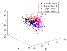
We now evaluate the proposed method with experiments on a synthetic data set and a real data set. The synthetic data set shown in Figure 4(a) consists of 400 normally distributed samples in 3superscript3\mathbb{R}^{3} from two classes. The two classes in each domain have different means, and the source and the target domains differ by a rotation of 90superscript9090^{\circ}. The variance of the normal distributions is chosen to be relatively large to ensure a sufficient level of difficulty. The COIL-20 object database [38] shown in Figure 4(b) consists of a total of 1440 images of 20 objects. Each object has 72 images taken from different camera angles rotating around it. We downsample the images to a resolution of 32×32323232\times 32 pixels. The 20 objects in the data set are divided into two groups and each object in the first group is matched to the object in the second group that is the most similar to it. Each group of 10 objects is taken as a different domain and the matched object pairs are considered to have the same class label in the experiments.
Refer to caption
(a) Synthetic data set
Refer to caption
(b) COIL-20 data set
Figure 4: (a) Synthetic data set with two classes drawn from normal distributions. (b) Sample images from the COIL-20 data set. Each source domain object in the upper row is assigned the same class label as the matching target domain object right below it.

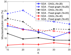
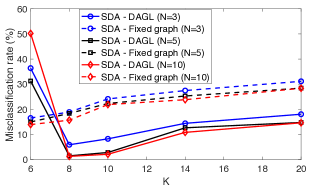
We first compare our SDA-DAGL algorithm with the SDA algorithm in order to study the efficiency of the proposed graph learning approach. In both data sets, we first independently construct the source and the target graphs by connecting each sample to its K𝐾K nearest neighbors and forming the weight matrices Wssuperscript𝑊𝑠W^{s} and Wtsuperscript𝑊𝑡W^{t} with a Gaussian kernel. The SDA algorithm uses the fixed graph topology represented by these weight matrices. In the proposed SDA-DAGL method, these weight matrices are used to initialize the algorithm as in Step 2 of Algorithm 1, and then they are refined gradually with the proposed joint graph learning and label estimation approach. All class labels are known in the source domain, while a small number of labels are known in the target domain. The class labels of the unlabeled target samples are estimated with the two algorithms in comparison. Figure 5 shows the variation of the misclassification rate of target samples with the number of neighbors (K𝐾K) for different numbers of labeled samples (N𝑁N) in the target domain. The results are averaged over around 10 random repetitions of the experiment with different selections of the labeled samples.

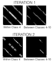
The results in Figure 5 show that the SDA-DAGL algorithm performs better than the SDA algorithm in almost all cases. This suggests that even if the SDA-DAGL algorithm is initialized with nonoptimal graphs, it can successfully learn a suitable pair of source and target graphs and accurately estimate the target labels. The performance of SDA-DAGL is seen to be robust to the choice of the initial number of neighbors K𝐾K in the synthetic data set in Figure 5(a), whereas it is more affected by the choice of K𝐾K in the COIL-20 data set in Figure 5(b). This is because the COIL-20 data set conforms quite well to a low-dimensional manifold structure due to the regular sampling of the camera rotation parameter generating the data set. Initializing the weight matrices with too high K𝐾K values leads to the loss of the information of the geometric structure from the beginning and makes it more difficult for the algorithm to recover the correct graph topologies along with the label estimates. The fact that too small K𝐾K values also yield large error in Figure 5(b) can be explained with the incompatibility of small K𝐾K values with the graph pruning strategy employed in our method. We also show in Figure 5(c) the evolution of the weight matrix Wtsuperscript𝑊𝑡W^{t} during two consecutive iterations of the SDA-DAGL method for the COIL-20 data set. The weights of the within-class edges in Class 4 and the between-class edges between Classes 4 and 10 are shown. The update on Wtsuperscript𝑊𝑡W^{t} is seen to mostly preserve the within-class edges, while it removes most of the between-class edges. Thus, the learnt graph topology is progressively improved.
Refer to caption
(a) Synthetic data set
Refer to caption
(b) COIL-20 data set
Refer to caption
(c) Target weight matrix
Figure 5: (a), (b) The variation of the misclassification rates of the target samples with the number of nearest neighbors K𝐾K. The curves with dashed lines are obtained with a fixed graph topology (SDA), whereas the corresponding curves with solid lines are obtained with the proposed graph learning method (SDA-DAGL). The results show that the graphs learnt with the proposed method yield higher performance than fixed graph topologies constructed with K-NN. (c) The evolution of Wtsuperscript𝑊𝑡W^{t} during two consecutive iterations. The black color represents 0 weight (no edge) and brighter tones indicate larger edge weights. The updates in the graph topology tend to preserve within-class edges and suppress between-class edges as desired.

We then study how the difference between the sizes of the source and the target graphs affects the algorithm performance. We fix the number Nssubscript𝑁𝑠N_{s} of source nodes, and vary the number Ntsubscript𝑁𝑡N_{t} of target nodes by constructing the target graph with a randomly selected subset of the target samples. The variation of the classification error with Ntsubscript𝑁𝑡N_{t} for different N𝑁N values (number of labeled target nodes) is presented in Table 1. The results show that the best performance is obtained when the source and the target graphs have an equal number of nodes (Nt=Nssubscript𝑁𝑡subscript𝑁𝑠N_{t}=N_{s}). In the synthetic data set, the removal of up to 25%percent2525\% of the target graph nodes is seen to be tolerable without much loss in the performance. On the other hand, the performance degrades more severely in the COIL-20 data set as the difference between the source and the target graph sizes increases. Due to the very particular geometric structure of this data set, the algorithm is more sensitive to the dissimilarity between the graph topologies.

Table 1: The variation of the target classification error with the number of target graph nodes. The classification performance tends to be higher when the source and the target graph sizes are similar.
Ntsubscript𝑁𝑡N_{t} 100 125 150 175 200
N=20𝑁20N=20 17.13 12.67 5.31 8.51 6.67
N=30𝑁30N=30 11.57 8.52 5.50 6.62 6.17
N=40𝑁40N=40 10.17 5.53 4.82 6.81 4.31

(a) Synthetic data set, Ns=200subscript𝑁𝑠200N_{s}=200

Ntsubscript𝑁𝑡N_{t} 30 40 50 60 72
N=3𝑁3N=3 28.22 25.08 22.42 17.79 6.52
N=5𝑁5N=5 27.44 24.11 15.60 14.15 1.13
N=10𝑁10N=10 22.70 18.67 16.85 5.76 1.06

(b) COIL-20 data set, Ns=72subscript𝑁𝑠72N_{s}=72

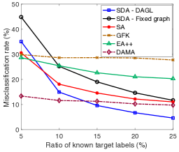
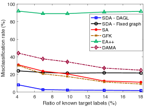
We finally present an overall comparison of the proposed SDA-DAGL method with some baseline domain adaptation methods representing different approaches. We compare our method to the Easy Adapt ++ (EA++) [8] algorithm based on feature augmentation; the Domain Adaptation using Manifold Alignment (DAMA) [10] algorithm which is a graph-based method learning a supervised embedding; and the Geodesic Flow Kernel (GFK) [11] and Subspace Alignment (SA) [12] methods, which align the PCA bases of the two domains via unsupervised projections. The misclassification rates of the algorithms on target samples are plotted with respect to the ratio of known target labels in Figures 6(a) and 6(b), respectively for the synthetic data set and the COIL-20 data sets. The misclassification error decreases as the ratio of the known target labels increases as expected. In both data sets, the proposed SDA-DAGL algorithm is often observed to outperform the baseline approaches and the SDA method, which uses a fixed graph topology. This suggests that the proposed graph learning strategy provides an effective solution for improving the performance of domain adaptation on graphs.
Refer to caption
(a) Synthetic data set
Refer to caption
(b) COIL-20 data set
Figure 6: The variation of the misclassification rate of the target samples with the ratio of labeled target samples. The proposed method is seen to outperform baseline approaches in most cases.

6 Conclusion

In this paper, we have studied the problem of domain adaptation on graphs both theoretically and methodologically. We have first proposed a theoretical analysis of the performance of graph domain adaptation methods. We have considered a setting where a pair of graphs are constructed from data samples drawn from a source manifold and a target manifold. We have focused on a graph domain adaptation framework where the source and the target label functions are estimated such that they have similar spectra. We have proposed an upper bound on the estimation error of the target label function and studied its dependence on the number of data samples, the geometric properties of the data manifolds, and graph parameters such as edge weights and the number of neighbors of graph nodes. In particular, as far as the graph properties are concerned, our theoretical results suggest that a “balanced” graph topology improves the performance of learning where the numbers of neighbors are proportionate across different nodes, and too weak edge weights and edges between too distant samples are avoided. Based on these findings, we then proposed a graph domain adaptation algorithm that jointly learns the graph structures and the label functions. Experimental results on synthetic and real data sets suggest that the proposed method yields promising performance in problems concerning machine learning on graph domains. An interesting future direction may be the extension of the study to multiple domains.

References

  • [1] M. Rohrbach, S. Ebert, and B. Schiele, “Transfer learning in a transductive setting,” in Proc. Advances in Neural Information Processing Systems, 2013, pp. 46–54.
  • [2] C. Wang and S. Mahadevan, “Manifold alignment using procrustes analysis,” in Proc. 25th Int. Conf. Machine Learning, 2008, pp. 1120–1127.
  • [3] M. Xiao and Y. Guo, “Feature space independent semi-supervised domain adaptation via kernel matching,” IEEE Trans. Pattern Anal. Mach. Intell., vol. 37, no. 1, pp. 54–66, 2015.
  • [4] Z. Fang and Z. Zhang, “Discriminative transfer learning on manifold,” in Proc. 13th SIAM Int. Conf. Data Mining, 2013, pp. 539–547.
  • [5] M. Pilancı and E. Vural, “Domain adaptation via transferring spectral properties of label functions on graphs,” in IEEE 12th Image, Video, and Multidimensional Signal Processing Workshop, 2016, pp. 1–5.
  • [6] J. Huang, A. J. Smola, A. Gretton, K. M. Borgwardt, and B. Schölkopf, “Correcting sample selection bias by unlabeled data,” in Proc. Advances in Neural Information Processing Systems 19, 2006, pp. 601–608.
  • [7] S. Khalighi, B. Ribeiro, and U. Nunes, “Importance weighted import vector machine for unsupervised domain adaptation,” IEEE Trans. Cybernetics, vol. 47, no. 10, pp. 3280–3292, 2017.
  • [8] H. Daumé, III, A. Kumar, and A. Saha, “Frustratingly easy semi-supervised domain adaptation,” in Proc. 2010 Workshop on Domain Adaptation for Natural Language Processing, 2010, pp. 53–59.
  • [9] L. Duan, D. Xu, and I. W. Tsang, “Learning with augmented features for heterogeneous domain adaptation,” in Proc. 29th International Conference on Machine Learning, 2012.
  • [10] C. Wang and S. Mahadevan, “Heterogeneous domain adaptation using manifold alignment,” in Proc. 22nd Int. Joint Conf. on Artificial Intelligence, 2011, pp. 1541–1546.
  • [11] B. Gong, Y. Shi, F. Sha, and K. Grauman, “Geodesic flow kernel for unsupervised domain adaptation,” in Proc. IEEE Conference on Computer Vision and Pattern Recognition, 2012, pp. 2066–2073.
  • [12] B. Fernando, A. Habrard, M. Sebban, and T. Tuytelaars, “Unsupervised visual domain adaptation using subspace alignment,” in Proc. IEEE International Conference on Computer Vision, 2013, ICCV ’13, pp. 2960–2967.
  • [13] M. Gong, K. Zhang, T. Liu, D. Tao, C. Glymour, and B. Schölkopf, “Domain adaptation with conditional transferable components,” in Proc. 33nd International Conference on Machine Learning, 2016, pp. 2839–2848.
  • [14] S. J. Pan, I. W. Tsang, J. T. Kwok, and Q. Yang, “Domain adaptation via transfer component analysis,” IEEE Trans. Neural Networks, vol. 22, no. 2, pp. 199–210, 2011.
  • [15] N. Courty, R. Flamary, D. Tuia, and A. Rakotomamonjy, “Optimal transport for domain adaptation,” IEEE Trans. Pattern Anal. Mach. Intell., vol. 39, no. 9, pp. 1853–1865, 2017.
  • [16] M. Jiang, W. Huang, Z. Huang, and G. G. Yen, “Integration of global and local metrics for domain adaptation learning via dimensionality reduction,” IEEE Trans. Cybernetics, vol. 47, no. 1, pp. 38–51, 2017.
  • [17] H. Yan, Y. Ding, P. Li, Q. Wang, Y. Xu, and W. Zuo, “Mind the class weight bias: Weighted maximum mean discrepancy for unsupervised domain adaptation,” in IEEE Conf. CVPR, 2017, pp. 945–954.
  • [18] T. Yao, Y. Pan, C. Ngo, H. Li, and T. Mei, “Semi-supervised domain adaptation with subspace learning for visual recognition,” in IEEE Conference on Computer Vision and Pattern Recognition, 2015, pp. 2142–2150.
  • [19] L. Cheng and S. J. Pan, “Semi-supervised domain adaptation on manifolds,” IEEE Trans. Neural Netw. Learning Syst., vol. 25, no. 12, pp. 2240–2249, 2014.
  • [20] D. Das and C. S. G. Lee, “Sample-to-sample correspondence for unsupervised domain adaptation,” Eng. Appl. of AI, vol. 73, pp. 80–91, 2018.
  • [21] D. Eynard, A. Kovnatsky, M. M. Bronstein, K. Glashoff, and A. M. Bronstein, “Multimodal manifold analysis by simultaneous diagonalization of Laplacians,” IEEE Trans. PAMI., vol. 37, no. 12, pp. 2505–2517, 2015.
  • [22] E. Rodolà, L. Cosmo, M. M. Bronstein, A. Torsello, and D. Cremers, “Partial functional correspondence,” Comput. Graph. Forum, vol. 36, no. 1, pp. 222–236, 2017.
  • [23] X. Dong, D. Thanou, P. Frossard, and P. Vandergheynst, “Learning Laplacian matrix in smooth graph signal representations,” IEEE Trans. Signal Processing, vol. 64, no. 23, pp. 6160–6173, 2016.
  • [24] V. Kalofolias, “How to learn a graph from smooth signals,” in Proc. Int. Conf. Artificial Intelligence and Statistics, 2016, pp. 920–929.
  • [25] H. E. Egilmez, E. Pavez, and A. Ortega, “Graph learning from data under Laplacian and structural constraints,” J. Sel. Topics Signal Processing, vol. 11, no. 6, pp. 825–841, 2017.
  • [26] A. Argyriou, M. Herbster, and M. Pontil, “Combining graph Laplacians for semi-supervised learning,” in Advances in Neural Information Processing Systems, 2005, pp. 67–74.
  • [27] G. Dai and D. Yeung, “Kernel selection forl semi-supervised kernel machines,” in Proc. Int. Conf. Machine Learning, 2007, pp. 185–192.
  • [28] C. Cortes, Y. Mansour, and M. Mohri, “Learning bounds for importance weighting,” in Proc. Advances in Neural Information Processing Systems 23, 2010, pp. 442–450.
  • [29] S. Ben-David, J. Blitzer, K. Crammer, and F. Pereira, “Analysis of representations for domain adaptation,” in Proc. Advances in Neural Information Processing Systems 19, 2006, pp. 137–144.
  • [30] J. Blitzer, K. Crammer, A. Kulesza, F. Pereira, and J. Wortman, “Learning bounds for domain adaptation,” in Proc. Advances in Neural Information Processing Systems 20, 2007, pp. 129–136.
  • [31] Y. Mansour, M. Mohri, and A. Rostamizadeh, “Domain adaptation: Learning bounds and algorithms,” in The 22nd Conference on Learning Theory, 2009.
  • [32] S. Ben-David, J. Blitzer, K. Crammer, A. Kulesza, F. Pereira, and J. Wortman, “A theory of learning from different domains,” Machine Learning, vol. 79, no. 1-2, pp. 151–175, 2010.
  • [33] C. Zhang, L. Zhang, and J. Ye, “Generalization bounds for domain adaptation,” arXiv preprint, 2013.
  • [34] F. R. K. Chung, Spectral Graph Theory, American Mathematical Society, 1997.
  • [35] D. I. Shuman, S. K. Narang, P. Frossard, A. Ortega, and P. Vandergheynst, “The emerging field of signal processing on graphs: Extending high-dimensional data analysis to networks and other irregular domains,” IEEE Signal Process. Mag., vol. 30, no. 3, pp. 83–98, 2013.
  • [36] M. Hein, J. Y. Audibert, and U. von Luxburg, “From graphs to manifolds - weak and strong pointwise consistency of graph Laplacians,” in 18th Annual Conference on Learning Theory, COLT, 2005, pp. 470–485.
  • [37] A. Singer, “From graph to manifold Laplacian: The convergence rate,” Applied and Computational Harmonic Analysis, vol. 21, no. 1, pp. 128 – 134, 2006.
  • [38] S. A. Nene, S. K. Nayar, and H. Murase, “Columbia Object Image Library (COIL-20),” Tech. Rep., Feb 1996.
  • [39] M. Pilancı and E. Vural, “Domain adaptation on graphs by learning aligned graph bases,” arXiv preprint, 2018, [Online]. Available: https://arxiv.org/abs/1803.05288.

Appendix A Proof of Theorem 1

In order to prove Theorem 1, we proceed as follows. We first propose an upper bound on the difference between the rates of variation of the source and target label functions in Section A.1. Next, we study the deviation between the eigenvalues of the source and target graph Laplacians in Section A.2. Finally, we combine these results in Section A.3 and present our upper bound on the estimation error of the target label function to finalize the proof.

A.1 Analysis of the difference between the rates of variation of the source and target label functions

We propose in Lemma 1 an upper bound on the difference between the rates of variation (f^s)TLsf^ssuperscriptsuperscript^𝑓𝑠𝑇superscript𝐿𝑠superscript^𝑓𝑠(\hat{f}^{s})^{T}L^{s}\hat{f}^{s} and (f^t)TLtf^tsuperscriptsuperscript^𝑓𝑡𝑇superscript𝐿𝑡superscript^𝑓𝑡(\hat{f}^{t})^{T}L^{t}\hat{f}^{t} of the estimated source and label functions on the graphs.

Lemma 1

Let 0=λ1sλ2sλRs0superscriptsubscript𝜆1𝑠superscriptsubscript𝜆2𝑠superscriptsubscript𝜆𝑅𝑠0=\lambda_{1}^{s}\leq\lambda_{2}^{s}\leq\dots\leq\lambda_{R}^{s} and 0=λ1tλ2tλRt0superscriptsubscript𝜆1𝑡superscriptsubscript𝜆2𝑡superscriptsubscript𝜆𝑅𝑡0=\lambda_{1}^{t}\leq\lambda_{2}^{t}\leq\dots\leq\lambda_{R}^{t} respectively denote the R𝑅R smallest eigenvalues of the source and target graph Laplacians Lssuperscript𝐿𝑠L^{s} and Ltsuperscript𝐿𝑡L^{t}. Assume that the deviation between the corresponding eigenvalues of the two graph Laplacians are bounded as |λisλit|δsuperscriptsubscript𝜆𝑖𝑠superscriptsubscript𝜆𝑖𝑡𝛿|\lambda_{i}^{s}-\lambda_{i}^{t}|\leq\delta, for all i=1,,R𝑖1𝑅i=1,\dots,R. Let the bandwidth parameter λR=max(λRs,λRt)subscript𝜆𝑅superscriptsubscript𝜆𝑅𝑠superscriptsubscript𝜆𝑅𝑡\lambda_{R}=\max(\lambda_{R}^{s},\lambda_{R}^{t}) indicate an upper bound for the frequencies of the first R𝑅R source and target Fourier basis vectors.

In the estimates f^s=U¯sα¯ssuperscript^𝑓𝑠superscript¯𝑈𝑠superscript¯𝛼𝑠\hat{f}^{s}=\overline{U}^{s}\overline{\alpha}^{s}, f^t=U¯tα¯tsuperscript^𝑓𝑡superscript¯𝑈𝑡superscript¯𝛼𝑡\hat{f}^{t}=\overline{U}^{t}\overline{\alpha}^{t} of the source and target label functions, let the difference between the Fourier coefficients of the label functions be bounded as α¯sα¯tΔαnormsuperscript¯𝛼𝑠superscript¯𝛼𝑡subscriptΔ𝛼\|\overline{\alpha}^{s}-\overline{\alpha}^{t}\|\leq\Delta_{\alpha}, and let C𝐶C be a bound on the norms of the coefficients such that α¯s,α¯tCnormsuperscript¯𝛼𝑠normsuperscript¯𝛼𝑡𝐶\|\overline{\alpha}^{s}\|,\|\overline{\alpha}^{t}\|\leq C.

Then the difference between the rates of variation of the source and target label function estimates on the graphs can be bounded as

|(f^s)TLsf^s(f^t)TLtf^t|C2δ+2CλRΔα.superscriptsuperscript^𝑓𝑠𝑇superscript𝐿𝑠superscript^𝑓𝑠superscriptsuperscript^𝑓𝑡𝑇superscript𝐿𝑡superscript^𝑓𝑡superscript𝐶2𝛿2𝐶subscript𝜆𝑅subscriptΔ𝛼\begin{split}|(\hat{f}^{s})^{T}L^{s}\hat{f}^{s}-(\hat{f}^{t})^{T}L^{t}\hat{f}^{t}|\leq C^{2}\delta&+2C\lambda_{R}\Delta_{\alpha}.\end{split}

The proof of Lemma 1 is an adaptation of the proof of [39, Proposition 1] to our case and it is given in Appendix B.1. Lemma 1 can be interpreted as follows: When the source and the target graphs are sufficiently similar, their graph Laplacians will have similar spectra, and the difference between their i𝑖i-th eigenvalues can be bounded as |λisλit|δsuperscriptsubscript𝜆𝑖𝑠superscriptsubscript𝜆𝑖𝑡𝛿|\lambda_{i}^{s}-\lambda_{i}^{t}|\leq\delta for a relatively small constant δ𝛿\delta. If in addition, the label functions vary sufficiently slowly to have limited bandwidth, then the source and target label functions have a similar rate of variation on the two graphs.

A.2 Analysis of the difference between the spectra of the source and target graphs

In Lemma 1 we have assumed that the source and target graph Laplacians have similar spectra, so that the difference |λisλit|superscriptsubscript𝜆𝑖𝑠superscriptsubscript𝜆𝑖𝑡|\lambda_{i}^{s}-\lambda_{i}^{t}| between their eigenvalues can be suitably bounded. We now determine under which conditions this is possible. We aim to develop an upper bound on |λisλit|superscriptsubscript𝜆𝑖𝑠superscriptsubscript𝜆𝑖𝑡|\lambda_{i}^{s}-\lambda_{i}^{t}| for all i𝑖i in terms of the properties of the data manifolds and the constructed graphs.

In domain adaptation problems, a one-to-one correspondence between the source and target data samples is often not available, in contrast to multi-view or multi-modal learning problems. Hence, we do not assume that there exists a particular relation between the samples xis=gs(γsi)superscriptsubscript𝑥𝑖𝑠superscript𝑔𝑠subscript𝛾subscript𝑠𝑖x_{i}^{s}=g^{s}(\gamma_{s_{i}}) and xit=gt(γti)superscriptsubscript𝑥𝑖𝑡superscript𝑔𝑡subscript𝛾subscript𝑡𝑖x_{i}^{t}=g^{t}(\gamma_{t_{i}}), such as being generated from the same parameter vector γsi=γtisubscript𝛾subscript𝑠𝑖subscript𝛾subscript𝑡𝑖\gamma_{s_{i}}=\gamma_{t_{i}} in the parameter space. Nevertheless, if the manifolds ssuperscript𝑠\mathcal{M}^{s} and tsuperscript𝑡\mathcal{M}^{t} defined over the same parameter space ΓΓ\Gamma are sampled under similar conditions (although independently), one may assume that the independently formed sample sets {xis}superscriptsubscript𝑥𝑖𝑠\{x_{i}^{s}\} and {xit}superscriptsubscript𝑥𝑖𝑡\{x_{i}^{t}\} can be reordered so that their corresponding parameter vectors {γis}superscriptsubscript𝛾𝑖𝑠\{\gamma_{i}^{s}\} and {γit}superscriptsubscript𝛾𝑖𝑡\{\gamma_{i}^{t}\} “fall” into nearby regions of the parameter space ΓΓ\Gamma. We state this assumption with the help of a cover

𝒞=m=1MBϵm(γm)Γ𝒞superscriptsubscript𝑚1𝑀subscript𝐵subscriptitalic-ϵ𝑚subscript𝛾𝑚Γ\mathcal{C}=\bigcup_{m=1}^{M}B_{\epsilon_{m}}(\gamma_{m})\subset\Gamma

in the parameter space, where Bϵ(γ)subscript𝐵italic-ϵ𝛾B_{\epsilon}(\gamma) denotes an open ball of radius ϵitalic-ϵ\epsilon around the parameter vector γ𝛾\gamma

Bϵ(γ)={γΓ:γγ<ϵ}subscript𝐵italic-ϵ𝛾conditional-setsuperscript𝛾Γnormsuperscript𝛾𝛾italic-ϵB_{\epsilon}(\gamma)=\{\gamma^{\prime}\in\Gamma:\|\gamma^{\prime}-\gamma\|<\epsilon\}

and the parameter vector of any data sample is in at least one ball in 𝒞𝒞\mathcal{C}

{γis}{γit}𝒞=m=1MBϵm(γm).superscriptsubscript𝛾𝑖𝑠superscriptsubscript𝛾𝑖𝑡𝒞superscriptsubscript𝑚1𝑀subscript𝐵subscriptitalic-ϵ𝑚subscript𝛾𝑚\{\gamma_{i}^{s}\}\cup\{\gamma_{i}^{t}\}\subset\mathcal{C}=\bigcup_{m=1}^{M}B_{\epsilon_{m}}(\gamma_{m}).

We assume without loss of generality that the source and target samples {xis}i=1Nsuperscriptsubscriptsuperscriptsubscript𝑥𝑖𝑠𝑖1𝑁\{x_{i}^{s}\}_{i=1}^{N} and {xit}i=1Nsuperscriptsubscriptsuperscriptsubscript𝑥𝑖𝑡𝑖1𝑁\{x_{i}^{t}\}_{i=1}^{N} are ordered such that for each i=1,,N𝑖1𝑁i=1,\dots,N,

γisBϵm(γm),γitBϵm(γm)formulae-sequencesuperscriptsubscript𝛾𝑖𝑠subscript𝐵subscriptitalic-ϵ𝑚subscript𝛾𝑚superscriptsubscript𝛾𝑖𝑡subscript𝐵subscriptitalic-ϵ𝑚subscript𝛾𝑚\gamma_{i}^{s}\in B_{\epsilon_{m}}(\gamma_{m}),\quad\quad\gamma_{i}^{t}\in B_{\epsilon_{m}}(\gamma_{m})

the samples γissuperscriptsubscript𝛾𝑖𝑠\gamma_{i}^{s} and γitsuperscriptsubscript𝛾𝑖𝑡\gamma_{i}^{t} are in the same ball Bϵm(γm)subscript𝐵subscriptitalic-ϵ𝑚subscript𝛾𝑚B_{\epsilon_{m}}(\gamma_{m}) for some m{1,,M}𝑚1𝑀m\in\{1,\dots,M\}. This condition imposes an ordering of the samples such that source and target samples with nearby indices correspond to nearby parameter vectors in the parameter space ΓΓ\Gamma.

Remarks: 1. First, let us note that when applying a graph-based domain adaptation algorithm, as the parameter-domain representation of the data samples is often unknown, it will not be possible to actually find such a reordering of the data. Nevertheless, our assumption of such a reordering is just for the purpose of theoretical analysis and is not needed in practice. This is because reordering the graph nodes will result in a permutation of the rows and the columns of the graph Laplacian. Since the permutations of the rows and columns with the same indices can be represented as the left and right multiplications of the graph Laplacian with the same symmetric rotation matrix, it will not change its eigenvalues. Hence, our analysis of the deviation |λisλit|superscriptsubscript𝜆𝑖𝑠superscriptsubscript𝜆𝑖𝑡|\lambda_{i}^{s}-\lambda_{i}^{t}| between the eigenvalues under the reordering assumption is still valid even if the nodes are not reordered in practice.

2. Second, notice that for a finite sampling of the source and target data, it is always possible to find such covers as mentioned above. However, the radii ϵ1,,ϵMsubscriptitalic-ϵ1subscriptitalic-ϵ𝑀\epsilon_{1},\dots,\epsilon_{M} of the open balls depend on the number of samples. In particular, the radii of these open sets decrease proportionally to the typical inter-sample distance between neighboring manifold samples as the number of samples N𝑁N increases, i.e., ϵm=O(N1/d)subscriptitalic-ϵ𝑚𝑂superscript𝑁1𝑑\epsilon_{m}=O(N^{-1/d}) where d𝑑d is the dimension of the manifolds s,tsuperscript𝑠superscript𝑡\mathcal{M}^{s},\mathcal{M}^{t}.

Next, we define some parameters regarding the properties of the graph. Let the source node xissuperscriptsubscript𝑥𝑖𝑠x_{i}^{s} have Kissuperscriptsubscript𝐾𝑖𝑠K_{i}^{s} neighbors in the source graph Gssuperscript𝐺𝑠G^{s}, where we denote xisxjssimilar-tosuperscriptsubscript𝑥𝑖𝑠superscriptsubscript𝑥𝑗𝑠x_{i}^{s}\sim x_{j}^{s} when xissuperscriptsubscript𝑥𝑖𝑠x_{i}^{s} and xjssuperscriptsubscript𝑥𝑗𝑠x_{j}^{s} are connected with an edge. Similarly let Kitsuperscriptsubscript𝐾𝑖𝑡K_{i}^{t} denote the number of neighbors of xitsuperscriptsubscript𝑥𝑖𝑡x_{i}^{t} in the target graph. Among the Kissuperscriptsubscript𝐾𝑖𝑠K_{i}^{s} neighbors xjssuperscriptsubscript𝑥𝑗𝑠x_{j}^{s} of xissuperscriptsubscript𝑥𝑖𝑠x_{i}^{s} in the source graph, some of their “correspondences” xjtsuperscriptsubscript𝑥𝑗𝑡x_{j}^{t} (with respect to the ordering discussed above) will be neighbors of the target node xitsuperscriptsubscript𝑥𝑖𝑡x_{i}^{t} corresponding to xissuperscriptsubscript𝑥𝑖𝑠x_{i}^{s}. Let βissuperscriptsubscript𝛽𝑖𝑠\beta_{i}^{s} be the proportion of such nodes, which is given by

βis=1Kis|{j:xjsxis,xjtxit}|superscriptsubscript𝛽𝑖𝑠1superscriptsubscript𝐾𝑖𝑠conditional-set𝑗formulae-sequencesimilar-tosuperscriptsubscript𝑥𝑗𝑠superscriptsubscript𝑥𝑖𝑠similar-tosuperscriptsubscript𝑥𝑗𝑡superscriptsubscript𝑥𝑖𝑡\beta_{i}^{s}=\frac{1}{K_{i}^{s}}\,|\{j:x_{j}^{s}\sim x_{i}^{s},x_{j}^{t}\sim x_{i}^{t}\}|

where |||\cdot| denotes the cardinality of a set. Similarly, let

βit=1Kit|{j:xjtxit,xjsxis}|.superscriptsubscript𝛽𝑖𝑡1superscriptsubscript𝐾𝑖𝑡conditional-set𝑗formulae-sequencesimilar-tosuperscriptsubscript𝑥𝑗𝑡superscriptsubscript𝑥𝑖𝑡similar-tosuperscriptsubscript𝑥𝑗𝑠superscriptsubscript𝑥𝑖𝑠\beta_{i}^{t}=\frac{1}{K_{i}^{t}}\,|\{j:x_{j}^{t}\sim x_{i}^{t},x_{j}^{s}\sim x_{i}^{s}\}|.

The more similar the source and target graphs are, the closer the parameters βis1superscriptsubscript𝛽𝑖𝑠1\beta_{i}^{s}\leq 1 and βit1superscriptsubscript𝛽𝑖𝑡1\beta_{i}^{t}\leq 1 will be to 111.

Finally, we define the parameter ϵ𝒩subscriptitalic-ϵ𝒩\epsilon_{\mathcal{N}} as

ϵ𝒩=max(maxxisxjsγisγjs,maxxitxjtγitγjt)subscriptitalic-ϵ𝒩subscriptsimilar-tosuperscriptsubscript𝑥𝑖𝑠superscriptsubscript𝑥𝑗𝑠normsuperscriptsubscript𝛾𝑖𝑠superscriptsubscript𝛾𝑗𝑠subscriptsimilar-tosuperscriptsubscript𝑥𝑖𝑡superscriptsubscript𝑥𝑗𝑡normsuperscriptsubscript𝛾𝑖𝑡superscriptsubscript𝛾𝑗𝑡\epsilon_{\mathcal{N}}=\max\left(\max_{x_{i}^{s}\sim x_{j}^{s}}\|\gamma_{i}^{s}-\gamma_{j}^{s}\|,\max_{x_{i}^{t}\sim x_{j}^{t}}\|\gamma_{i}^{t}-\gamma_{j}^{t}\|\right)

which gives the largest possible parameter domain distance between two neighboring nodes in the source or target graphs. Also, due to our assumption on the ordering of the samples, for any i𝑖i, there exists some m{1,,M}𝑚1𝑀m\in\{1,\dots,M\} such that γis,γitBϵm(γm)superscriptsubscript𝛾𝑖𝑠superscriptsubscript𝛾𝑖𝑡subscript𝐵subscriptitalic-ϵ𝑚subscript𝛾𝑚\gamma_{i}^{s},\gamma_{i}^{t}\in B_{\epsilon_{m}}(\gamma_{m}). Let

ϵmi=min{ϵm:γis,γitBϵm(γm)}subscriptitalic-ϵsubscript𝑚𝑖:subscriptitalic-ϵ𝑚superscriptsubscript𝛾𝑖𝑠superscriptsubscript𝛾𝑖𝑡subscript𝐵subscriptitalic-ϵ𝑚subscript𝛾𝑚\epsilon_{m_{i}}=\min\{\epsilon_{m}:\gamma_{i}^{s},\gamma_{i}^{t}\in B_{\epsilon_{m}}(\gamma_{m})\}

and also let

ϵΓ=ϵ𝒩+2maxiϵmisubscriptitalic-ϵΓsubscriptitalic-ϵ𝒩2subscript𝑖subscriptitalic-ϵsubscript𝑚𝑖\epsilon_{\Gamma}=\epsilon_{\mathcal{N}}+2\max_{i}\epsilon_{m_{i}}

represent a generic upper bound on the parameter domain distance between “within-domain” and “cross-domain” neighboring samples.

We are now ready to state our bound on the deviation |λisλit|superscriptsubscript𝜆𝑖𝑠superscriptsubscript𝜆𝑖𝑡|\lambda_{i}^{s}-\lambda_{i}^{t}| between the corresponding eigenvalues of the source and target graph Laplacians in Lemma 2.

Lemma 2

Let Lssuperscript𝐿𝑠L^{s} and Ltsuperscript𝐿𝑡L^{t} be the Laplacian matrices of the source and target graphs with respective eigenvalues ordered as 0=λ1sλ2sλNs0superscriptsubscript𝜆1𝑠superscriptsubscript𝜆2𝑠superscriptsubscript𝜆𝑁𝑠0=\lambda_{1}^{s}\leq\lambda_{2}^{s}\leq\dots\leq\lambda_{N}^{s}, and 0=λ1tλ2tλNt0superscriptsubscript𝜆1𝑡superscriptsubscript𝜆2𝑡superscriptsubscript𝜆𝑁𝑡0=\lambda_{1}^{t}\leq\lambda_{2}^{t}\leq\dots\leq\lambda_{N}^{t}. Based on the above definitions of the graph parameters, let us denote

ΔW:=Lϕ(AMs+Ms+Mt)ϵΓ.assignsubscriptΔ𝑊subscript𝐿italic-ϕ𝐴subscript𝑀𝑠subscript𝑀𝑠subscript𝑀𝑡subscriptitalic-ϵΓ\Delta_{W}:=L_{\phi}\,(A\,M_{s}+M_{s}+M_{t})\epsilon_{\Gamma}.

Then for all i=1,,N𝑖1𝑁i=1,\dots,N the deviation |λisλit|superscriptsubscript𝜆𝑖𝑠superscriptsubscript𝜆𝑖𝑡|\lambda_{i}^{s}-\lambda_{i}^{t}| between the corresponding eigenvalues of Lssuperscript𝐿𝑠L^{s} and Ltsuperscript𝐿𝑡L^{t} is upper bounded as

|λisλit|ρmax:=maxi=1,,N 2(βisKisΔW+(1βis)Kisϕ0+(1βit)Kitϕ0).superscriptsubscript𝜆𝑖𝑠superscriptsubscript𝜆𝑖𝑡subscript𝜌assignsubscript𝑖1𝑁2superscriptsubscript𝛽𝑖𝑠superscriptsubscript𝐾𝑖𝑠subscriptΔ𝑊1superscriptsubscript𝛽𝑖𝑠superscriptsubscript𝐾𝑖𝑠subscriptitalic-ϕ01superscriptsubscript𝛽𝑖𝑡superscriptsubscript𝐾𝑖𝑡subscriptitalic-ϕ0|\lambda_{i}^{s}-\lambda_{i}^{t}|\leq\rho_{\max}:=\max_{i=1,\dots,N}\,2\left(\beta_{i}^{s}K_{i}^{s}\Delta_{W}+(1-\beta_{i}^{s})K_{i}^{s}\phi_{0}+(1-\beta_{i}^{t})K_{i}^{t}\phi_{0}\right).

The proof of Lemma 2 is presented in Appendix B.2. Lemma 2 can be interpreted as follows. First, recall that the parameters βissuperscriptsubscript𝛽𝑖𝑠\beta_{i}^{s} and βitsuperscriptsubscript𝛽𝑖𝑡\beta_{i}^{t} give the ratio of the source and target neighbors of a graph node that have correspondences in the other graph. Hence, they provide a measure of the similarity between the source and the target graphs. When the resemblance between the source and target graphs gets stronger, these parameters get closer to 111. If we consider the asymptotic case where βissuperscriptsubscript𝛽𝑖𝑠\beta_{i}^{s} and βitsuperscriptsubscript𝛽𝑖𝑡\beta_{i}^{t} approach 111, the upper bound ρmaxsubscript𝜌\rho_{\max} on the deviation between the eigenvalues becomes

limβis1,βit1ρmax=maxi 2KisΔW.subscriptformulae-sequencesuperscriptsubscript𝛽𝑖𝑠1superscriptsubscript𝛽𝑖𝑡1subscript𝜌subscript𝑖2superscriptsubscript𝐾𝑖𝑠subscriptΔ𝑊\lim_{\beta_{i}^{s}\rightarrow 1,\,\beta_{i}^{t}\rightarrow 1}\rho_{\max}=\max_{i}\,2K_{i}^{s}\Delta_{W}.

In order to understand how the eigenvalue deviation changes with the sampling density of the graphs, we can study the variation of this term with the number N𝑁N of graph nodes. Assuming that the number of neighbors Kissuperscriptsubscript𝐾𝑖𝑠K_{i}^{s} are of O(1)𝑂1O(1) with respect to N𝑁N, i.e., if the number of neighbors is not increased proportionally to N𝑁N in the graph construction, the rate of variation of ρmaxsubscript𝜌\rho_{\max} with N𝑁N is given by that of the term ΔWsubscriptΔ𝑊\Delta_{W}. As the number N𝑁N of data points sampled from the manifolds ssuperscript𝑠\mathcal{M}^{s}, tsuperscript𝑡\mathcal{M}^{t} increases, we have

ϵmi,ϵ𝒩=O(N1/d)subscriptitalic-ϵsubscript𝑚𝑖subscriptitalic-ϵ𝒩𝑂superscript𝑁1𝑑\epsilon_{m_{i}},\epsilon_{\mathcal{N}}=O(N^{-1/d})

and consequently, ϵΓ=O(N1/d)subscriptitalic-ϵΓ𝑂superscript𝑁1𝑑\epsilon_{\Gamma}=O(N^{-1/d}), where d𝑑d is the intrinsic dimension of the manifolds. This yields ΔW=O(N1/d)subscriptΔ𝑊𝑂superscript𝑁1𝑑\Delta_{W}=O(N^{-1/d}), hence, we obtain

|λisλit|ρmax=O(N1/d)superscriptsubscript𝜆𝑖𝑠superscriptsubscript𝜆𝑖𝑡subscript𝜌𝑂superscript𝑁1𝑑|\lambda_{i}^{s}-\lambda_{i}^{t}|\leq\rho_{\max}=O(N^{-1/d})

for the asymptotic case βis1,βit1formulae-sequencesuperscriptsubscript𝛽𝑖𝑠1superscriptsubscript𝛽𝑖𝑡1\beta_{i}^{s}\rightarrow 1,\,\beta_{i}^{t}\rightarrow 1.

Next, we can also interpret Lemma 2 from the perspective of the similarity between the manifolds. As the geometric structures of the source and target manifolds ssuperscript𝑠\mathcal{M}^{s}, tsuperscript𝑡\mathcal{M}^{t} get more similar, the constants Alsubscript𝐴𝑙A_{l} and Ausubscript𝐴𝑢A_{u} will approach 111, and the constant A𝐴A will approach 0. We observe that this reduces the deviation |λisλit|superscriptsubscript𝜆𝑖𝑠superscriptsubscript𝜆𝑖𝑡|\lambda_{i}^{s}-\lambda_{i}^{t}| as ΔWsubscriptΔ𝑊\Delta_{W} is proportional to A𝐴A. Also, as the Lipschitz regularity of the functions gssuperscript𝑔𝑠g^{s}, gtsuperscript𝑔𝑡g^{t} defining the source and target manifolds improves, the constants Mssubscript𝑀𝑠M_{s} and Mtsubscript𝑀𝑡M_{t} will decrease, hence, ΔWsubscriptΔ𝑊\Delta_{W} will also decrease. We can summarize these with the observation that as Ms,Mt0subscript𝑀𝑠subscript𝑀𝑡0M_{s},M_{t}\rightarrow 0, A0𝐴0A\rightarrow 0, and βis,βit1superscriptsubscript𝛽𝑖𝑠superscriptsubscript𝛽𝑖𝑡1\beta_{i}^{s},\beta_{i}^{t}\rightarrow 1, the eigenvalue difference converges to 0 as |λisλit|0superscriptsubscript𝜆𝑖𝑠superscriptsubscript𝜆𝑖𝑡0|\lambda_{i}^{s}-\lambda_{i}^{t}|\rightarrow 0 for all i=1,,N.𝑖1𝑁i=1,\dots,N.

A.3 Bounding the estimation error of the target label function

Putting together the results from Lemmas 1 and 2, we arrive at the following observation: Assuming that the conditions of Lemma 2 hold, the spectrum perturbation parameter δ𝛿\delta in Lemma 1 can be upper bounded as δρmax𝛿subscript𝜌\delta\leq\rho_{\max}. In this case, the rates of variations of the source and target function estimates differ as

|(f^s)TLsf^s(f^t)TLtf^t|C2ρmax+2CλRΔα.superscriptsuperscript^𝑓𝑠𝑇superscript𝐿𝑠superscript^𝑓𝑠superscriptsuperscript^𝑓𝑡𝑇superscript𝐿𝑡superscript^𝑓𝑡superscript𝐶2subscript𝜌2𝐶subscript𝜆𝑅subscriptΔ𝛼|(\hat{f}^{s})^{T}L^{s}\hat{f}^{s}-(\hat{f}^{t})^{T}L^{t}\hat{f}^{t}|\leq C^{2}\rho_{\max}+2C\lambda_{R}\Delta_{\alpha}.

Due to our assumption fs=f^ssuperscript𝑓𝑠superscript^𝑓𝑠f^{s}=\hat{f}^{s}, the above inequality implies

(f^t)TLtf^tB^=(fs)TLsfs+C2ρmax+2CλRΔα.superscriptsuperscript^𝑓𝑡𝑇superscript𝐿𝑡superscript^𝑓𝑡^𝐵superscriptsuperscript𝑓𝑠𝑇superscript𝐿𝑠superscript𝑓𝑠superscript𝐶2subscript𝜌2𝐶subscript𝜆𝑅subscriptΔ𝛼(\hat{f}^{t})^{T}L^{t}\hat{f}^{t}\leq\hat{B}=(f^{s})^{T}L^{s}f^{s}+C^{2}\rho_{\max}+2C\lambda_{R}\Delta_{\alpha}.

The parameter B^^𝐵\hat{B} thus gives a bound on the rate of variation of the label function estimate f^tsuperscript^𝑓𝑡\hat{f}^{t} on the graph. Recall also the assumption on the true target label function in Theorem 1

(ft)TLtftB.superscriptsuperscript𝑓𝑡𝑇superscript𝐿𝑡superscript𝑓𝑡𝐵(f^{t})^{T}L^{t}f^{t}\leq B.

Under these assumptions, we would like to find an upper bound on the target label estimation error f^tftnormsuperscript^𝑓𝑡superscript𝑓𝑡\|\hat{f}^{t}-f^{t}\|.

Before we state our bound on the estimation error, we first define some parameters related to the properties of the target graph. First, recall from Section 3.2 that we consider a setting where very few labels yit=ft(xit)subscriptsuperscript𝑦𝑡𝑖superscript𝑓𝑡subscriptsuperscript𝑥𝑡𝑖y^{t}_{i}=f^{t}(x^{t}_{i}) are known on the target graph, with indices iILt{1,,Nt}𝑖superscriptsubscript𝐼𝐿𝑡1subscript𝑁𝑡i\in I_{L}^{t}\subset\{1,\dots,N_{t}\} in the index set ILtsuperscriptsubscript𝐼𝐿𝑡I_{L}^{t}. Now let us denote the set of indices of the unlabeled nodes of the target graph as IUt=ItILt,superscriptsubscript𝐼𝑈𝑡superscript𝐼𝑡superscriptsubscript𝐼𝐿𝑡I_{U}^{t}=I^{t}\setminus I_{L}^{t}, where It={1,,Nt}superscript𝐼𝑡1subscript𝑁𝑡I^{t}=\{1,\dots,N_{t}\} denotes the set of all target node indices and \cdot\setminus\cdot denotes the set difference. Moreover, assuming that the target graph is connected, or otherwise each connected component contains at least one labeled node, one can partition the node indices as It=ILtIU1tIUQt,superscript𝐼𝑡superscriptsubscript𝐼𝐿𝑡superscriptsubscript𝐼subscript𝑈1𝑡superscriptsubscript𝐼subscript𝑈𝑄𝑡I^{t}=I_{L}^{t}\cup I_{U_{1}}^{t}\cup\dots\cup I_{U_{Q}}^{t}, where IUqtsuperscriptsubscript𝐼subscript𝑈𝑞𝑡I_{U_{q}}^{t} consists of the indices of unlabeled nodes that are connected to the nearest labeled node through a shortest path of length q𝑞q (with q𝑞q hops). Q𝑄Q is then the longest possible length of the shortest path between an unlabeled and a labeled node. Let IU0t:=ILtassignsuperscriptsubscript𝐼subscript𝑈0𝑡superscriptsubscript𝐼𝐿𝑡I_{U_{0}}^{t}:=I_{L}^{t} simply stand for the index set of labeled nodes. We thus partition the target graph nodes in sets of several “layers” q=0,1,,Q𝑞01𝑄q=0,1,\dots,Q, with respect to their proximity to the closest labeled node.

Let 𝒩jq:={iIUqt:xitxjt}assignsuperscriptsubscript𝒩𝑗𝑞conditional-set𝑖superscriptsubscript𝐼subscript𝑈𝑞𝑡similar-tosuperscriptsubscript𝑥𝑖𝑡superscriptsubscript𝑥𝑗𝑡\mathcal{N}_{j}^{q}:=\{i\in I_{U_{q}}^{t}:x_{i}^{t}\sim x_{j}^{t}\} denote the set of indices of the neighbors of a node xjtsuperscriptsubscript𝑥𝑗𝑡x_{j}^{t} within the nodes of layer q𝑞q, where similar-to\sim denotes neighboring nodes. We can define the parameters Kqmin:=minjIUqt|𝒩jq1|assignsuperscriptsubscript𝐾𝑞subscript𝑗superscriptsubscript𝐼subscript𝑈𝑞𝑡superscriptsubscript𝒩𝑗𝑞1{K_{q}^{\min}}:=\min_{j\in I_{U_{q}}^{t}}|\mathcal{N}_{j}^{q-1}| and Kqmax:=maxjIUqt|𝒩jq+1|,assignsuperscriptsubscript𝐾𝑞subscript𝑗superscriptsubscript𝐼subscript𝑈𝑞𝑡superscriptsubscript𝒩𝑗𝑞1{K_{q}^{\max}}:=\max_{j\in I_{U_{q}}^{t}}|\mathcal{N}_{j}^{q+1}|, where |||\cdot| denotes the cardinality. Kqminsuperscriptsubscript𝐾𝑞{K_{q}^{\min}} is thus the minimum number of neighbors between a layer q𝑞q and its preceding layer q1𝑞1q-1, and Kqmaxsuperscriptsubscript𝐾𝑞{K_{q}^{\max}} is the maximum number of neighbors between a layer q𝑞q and its succeeding layer q+1𝑞1q+1. Let us also define the minimum weight of an edge between any two nodes from consecutive layers as wmin:=minq=1,,Qwqmin,assignsuperscript𝑤subscript𝑞1𝑄subscriptsuperscript𝑤𝑞w^{\min}:=\min_{q=1,\dots,Q}w^{\min}_{q}, where wqmin=min{Wijt:xitxjt,iIUqt,jIUq1t}subscriptsuperscript𝑤𝑞:subscriptsuperscript𝑊𝑡𝑖𝑗formulae-sequencesimilar-tosuperscriptsubscript𝑥𝑖𝑡superscriptsubscript𝑥𝑗𝑡formulae-sequence𝑖superscriptsubscript𝐼subscript𝑈𝑞𝑡𝑗superscriptsubscript𝐼subscript𝑈𝑞1𝑡w^{\min}_{q}=\min\{W^{t}_{ij}:x_{i}^{t}\sim x_{j}^{t},\,i\in I_{U_{q}}^{t},\,j\in I_{U_{q-1}}^{t}\} is the smallest edge weight between layers q𝑞q and q1𝑞1q-1.

Our derivation of an upper bound on the target label estimation error is based on the following decomposition

f^tft2=q=0Qf^UqtfUqt2superscriptnormsuperscript^𝑓𝑡superscript𝑓𝑡2superscriptsubscript𝑞0𝑄superscriptnormsubscriptsuperscript^𝑓𝑡subscript𝑈𝑞subscriptsuperscript𝑓𝑡subscript𝑈𝑞2\|\hat{f}^{t}-f^{t}\|^{2}=\sum_{q=0}^{Q}\|\hat{f}^{t}_{U_{q}}-f^{t}_{U_{q}}\|^{2}

where the vectors fUqtsubscriptsuperscript𝑓𝑡subscript𝑈𝑞f^{t}_{U_{q}} and f^Uqtsubscriptsuperscript^𝑓𝑡subscript𝑈𝑞\hat{f}^{t}_{U_{q}} are respectively obtained by restricting the vectors ftsuperscript𝑓𝑡f^{t} and f^tsuperscript^𝑓𝑡\hat{f}^{t} to their entries in the index set IUqtsuperscriptsubscript𝐼subscript𝑈𝑞𝑡I_{U_{q}}^{t}. Our strategy for bounding the target error is to bound the error of each layer in terms of the error of the previous layer, and use the observation that the error of layer q=0𝑞0q=0 is 00 as it consists of the labeled samples. In the following result, we first provide an upper bound on the error f^UqtfUqt2superscriptnormsubscriptsuperscript^𝑓𝑡subscript𝑈𝑞subscriptsuperscript𝑓𝑡subscript𝑈𝑞2\|\hat{f}^{t}_{U_{q}}-f^{t}_{U_{q}}\|^{2} of the q𝑞q-th layer in terms of the error f^Uq1tfUq1t2superscriptnormsubscriptsuperscript^𝑓𝑡subscript𝑈𝑞1subscriptsuperscript𝑓𝑡subscript𝑈𝑞12\|\hat{f}^{t}_{U_{q-1}}-f^{t}_{U_{q-1}}\|^{2} of the preceding layer q1𝑞1q-1.

Lemma 3

Let

Bq:=jIUqtxitxjt,iIUq1tWijt(fitfjt)2assignsubscript𝐵𝑞subscript𝑗superscriptsubscript𝐼subscript𝑈𝑞𝑡subscriptformulae-sequencesimilar-tosuperscriptsubscript𝑥𝑖𝑡superscriptsubscript𝑥𝑗𝑡𝑖superscriptsubscript𝐼subscript𝑈𝑞1𝑡superscriptsubscript𝑊𝑖𝑗𝑡superscriptsubscriptsuperscript𝑓𝑡𝑖subscriptsuperscript𝑓𝑡𝑗2B_{q}:=\sum_{j\in I_{U_{q}}^{t}}\ \sum_{x_{i}^{t}\sim x_{j}^{t},\ i\in I_{U_{q-1}}^{t}}W_{ij}^{t}(f^{t}_{i}-f^{t}_{j})^{2}

denote the total rate of variation of the true target label function ftsuperscript𝑓𝑡f^{t} over the edges between two consecutive layers q𝑞q and q1𝑞1q-1. Similarly define

B^q:=jIUqtxitxjt,iIUq1tWijt(f^itf^jt)2assignsubscript^𝐵𝑞subscript𝑗superscriptsubscript𝐼subscript𝑈𝑞𝑡subscriptformulae-sequencesimilar-tosuperscriptsubscript𝑥𝑖𝑡superscriptsubscript𝑥𝑗𝑡𝑖superscriptsubscript𝐼subscript𝑈𝑞1𝑡superscriptsubscript𝑊𝑖𝑗𝑡superscriptsubscriptsuperscript^𝑓𝑡𝑖subscriptsuperscript^𝑓𝑡𝑗2\hat{B}_{q}:=\sum_{j\in I_{U_{q}}^{t}}\ \sum_{x_{i}^{t}\sim x_{j}^{t},\ i\in I_{U_{q-1}}^{t}}W_{ij}^{t}(\hat{f}^{t}_{i}-\hat{f}^{t}_{j})^{2}

for the estimate f^tsuperscript^𝑓𝑡\hat{f}^{t} of the target label function. We can then bound the estimation error of the q𝑞q-th layer in terms of the estimation error of the preceding layer q1𝑞1q-1 as

f^UqtfUqt2|IUqt|Kqmin(Bq+B^qwqmin+Kq1maxf^Uq1tfUq1t)2superscriptnormsubscriptsuperscript^𝑓𝑡subscript𝑈𝑞subscriptsuperscript𝑓𝑡subscript𝑈𝑞2superscriptsubscript𝐼subscript𝑈𝑞𝑡superscriptsubscript𝐾𝑞superscriptsubscript𝐵𝑞subscript^𝐵𝑞subscriptsuperscript𝑤𝑞superscriptsubscript𝐾𝑞1normsubscriptsuperscript^𝑓𝑡subscript𝑈𝑞1subscriptsuperscript𝑓𝑡subscript𝑈𝑞12\|\hat{f}^{t}_{U_{q}}-f^{t}_{U_{q}}\|^{2}\leq\frac{|I_{U_{q}}^{t}|}{{K_{q}^{\min}}}\left(\frac{\sqrt{B_{q}}+\sqrt{\hat{B}_{q}}}{\sqrt{w^{\min}_{q}}}+\sqrt{{K_{q-1}^{\max}}}\ \|\hat{f}^{t}_{U_{q-1}}-f^{t}_{U_{q-1}}\|\right)^{2}

for q=1,,Q𝑞1𝑄q=1,\dots,Q.

The proof of Lemma 3 is given in Appendix B.3.

Lemma 3 provides an upper bound on the error of each layer in terms of the error of the previous layer. We can now use this result to obtain an upper bound on the overall target label estimation error, which is presented in the following lemma.

Lemma 4

The estimation error of the target label function can be bounded as

ftf^t2κwmin(B+B^)2superscriptnormsuperscript𝑓𝑡superscript^𝑓𝑡2𝜅superscript𝑤superscript𝐵^𝐵2\|f^{t}-\hat{f}^{t}\|^{2}\leq\frac{\kappa}{w^{\min}}(\sqrt{B}+\sqrt{\hat{B}})^{2}

where

κ=q=1Q|IUqt|Kqmin(1+l=1q1m=lq1|IUmt|KmmaxKmmin).𝜅superscriptsubscript𝑞1𝑄superscriptsubscript𝐼subscript𝑈𝑞𝑡superscriptsubscript𝐾𝑞1superscriptsubscript𝑙1𝑞1superscriptsubscriptproduct𝑚𝑙𝑞1superscriptsubscript𝐼subscript𝑈𝑚𝑡superscriptsubscript𝐾𝑚superscriptsubscript𝐾𝑚\kappa=\sum_{q=1}^{Q}\frac{|I_{U_{q}}^{t}|}{{K_{q}^{\min}}}\left(1+\sum_{l=1}^{q-1}\prod_{m=l}^{q-1}|I_{U_{m}}^{t}|\frac{K_{m}^{\max}}{K_{m}^{\min}}\right).

The proof of Lemma 4 is given in Appendix B.4.

The results stated in Lemmas 1-4 provide a complete characterization of the performance of estimating the target label function in a graph domain adaptation setting. We are now ready to combine these results in the following main result.

Theorem 2

Consider a graph-based domain adaptation algorithm matching the spectra of the source and target label functions f^s=U¯sα¯ssuperscript^𝑓𝑠superscript¯𝑈𝑠superscript¯𝛼𝑠\hat{f}^{s}=\overline{U}^{s}\overline{\alpha}^{s} and f^t=U¯tα¯tsuperscript^𝑓𝑡superscript¯𝑈𝑡superscript¯𝛼𝑡\hat{f}^{t}=\overline{U}^{t}\overline{\alpha}^{t} such that the difference between the Fourier coefficients of the label functions are bounded as α¯sα¯tΔαnormsuperscript¯𝛼𝑠superscript¯𝛼𝑡subscriptΔ𝛼\|\overline{\alpha}^{s}-\overline{\alpha}^{t}\|\leq\Delta_{\alpha}, the norms of the Fourier coefficients are bounded as α¯s,α¯tCnormsuperscript¯𝛼𝑠normsuperscript¯𝛼𝑡𝐶\|\overline{\alpha}^{s}\|,\|\overline{\alpha}^{t}\|\leq C, and f^ssuperscript^𝑓𝑠\hat{f}^{s} and f^tsuperscript^𝑓𝑡\hat{f}^{t} are band-limited on the graphs so as not to contain any components with frequencies larger than λRsubscript𝜆𝑅\lambda_{R}.

Assume the source and target graphs are constructed independently from equally many data samples by setting the graph weights via the kernel ϕitalic-ϕ\phi, where the source samples {xis}i=1Nsuperscriptsubscriptsuperscriptsubscript𝑥𝑖𝑠𝑖1𝑁\{x_{i}^{s}\}_{i=1}^{N} and target samples {xit}i=1Nsuperscriptsubscriptsuperscriptsubscript𝑥𝑖𝑡𝑖1𝑁\{x_{i}^{t}\}_{i=1}^{N} are drawn from the manifolds ssuperscript𝑠\mathcal{M}^{s} and tsuperscript𝑡\mathcal{M}^{t} defined via the functions gssuperscript𝑔𝑠g^{s} and gtsuperscript𝑔𝑡g^{t} over a common parameter domain ΓΓ\Gamma. Let

ΔW=Lϕ(AMs+Ms+Mt)ϵΓ.subscriptΔ𝑊subscript𝐿italic-ϕ𝐴subscript𝑀𝑠subscript𝑀𝑠subscript𝑀𝑡subscriptitalic-ϵΓ\Delta_{W}=L_{\phi}\,(A\,M_{s}+M_{s}+M_{t})\,\epsilon_{\Gamma}. (10)

and

ρmax=maxi=1,,N 2(βisKisΔW+(1βis)Kisϕ0+(1βit)Kitϕ0).subscript𝜌subscript𝑖1𝑁2superscriptsubscript𝛽𝑖𝑠superscriptsubscript𝐾𝑖𝑠subscriptΔ𝑊1superscriptsubscript𝛽𝑖𝑠superscriptsubscript𝐾𝑖𝑠subscriptitalic-ϕ01superscriptsubscript𝛽𝑖𝑡superscriptsubscript𝐾𝑖𝑡subscriptitalic-ϕ0\rho_{\max}=\max_{i=1,\dots,N}\,2\left(\beta_{i}^{s}K_{i}^{s}\Delta_{W}+(1-\beta_{i}^{s})K_{i}^{s}\phi_{0}+(1-\beta_{i}^{t})K_{i}^{t}\phi_{0}\right). (11)

Then, the difference between the rates of variation of the source and target function estimates is upper bounded as

|(f^s)TLsf^s(f^t)TLtf^t|C2ρmax+2CλRΔα.superscriptsuperscript^𝑓𝑠𝑇superscript𝐿𝑠superscript^𝑓𝑠superscriptsuperscript^𝑓𝑡𝑇superscript𝐿𝑡superscript^𝑓𝑡superscript𝐶2subscript𝜌2𝐶subscript𝜆𝑅subscriptΔ𝛼|(\hat{f}^{s})^{T}L^{s}\hat{f}^{s}-(\hat{f}^{t})^{T}L^{t}\hat{f}^{t}|\leq C^{2}\rho_{\max}+2C\lambda_{R}\Delta_{\alpha}.

Moreover, if f^s=fssuperscript^𝑓𝑠superscript𝑓𝑠\hat{f}^{s}=f^{s} and if the target label function estimates f^itsubscriptsuperscript^𝑓𝑡𝑖\hat{f}^{t}_{i} are equal to the true labels fitsubscriptsuperscript𝑓𝑡𝑖f^{t}_{i} at labeled nodes, the target label estimation error can be bounded as

f^tft2κwmin(B+B^)2superscriptnormsuperscript^𝑓𝑡superscript𝑓𝑡2𝜅superscript𝑤superscript𝐵^𝐵2\|\hat{f}^{t}-f^{t}\|^{2}\leq\frac{\kappa}{w^{\min}}(\sqrt{B}+\sqrt{\hat{B}})^{2} (12)

where

B^=(fs)TLsfs+C2ρmax+2CλRΔα,^𝐵superscriptsuperscript𝑓𝑠𝑇superscript𝐿𝑠superscript𝑓𝑠superscript𝐶2subscript𝜌2𝐶subscript𝜆𝑅subscriptΔ𝛼\hat{B}=(f^{s})^{T}L^{s}f^{s}+C^{2}\rho_{\max}+2C\lambda_{R}\Delta_{\alpha}, (13)

B𝐵B is an upper bound on the rate of variation of the true label function

(ft)TLtftB,superscriptsuperscript𝑓𝑡𝑇superscript𝐿𝑡superscript𝑓𝑡𝐵(f^{t})^{T}L^{t}f^{t}\leq B, (14)

and

κ=q=1Q|IUqt|Kqmin(1+l=1q1m=lq1|IUmt|KmmaxKmmin).𝜅superscriptsubscript𝑞1𝑄superscriptsubscript𝐼subscript𝑈𝑞𝑡superscriptsubscript𝐾𝑞1superscriptsubscript𝑙1𝑞1superscriptsubscriptproduct𝑚𝑙𝑞1superscriptsubscript𝐼subscript𝑈𝑚𝑡superscriptsubscript𝐾𝑚superscriptsubscript𝐾𝑚\kappa=\sum_{q=1}^{Q}\frac{|I_{U_{q}}^{t}|}{{K_{q}^{\min}}}\left(1+\sum_{l=1}^{q-1}\prod_{m=l}^{q-1}|I_{U_{m}}^{t}|\frac{K_{m}^{\max}}{K_{m}^{\min}}\right).

We finally conclude the proof of Theorem 1 by observing that it is simply a summarizing restatement of the result in Theorem 2.

Appendix B Proofs of the Lemmas in Appendix A

B.1 Proof of Lemma 1

Proof.

The rates of variation of f^ssuperscript^𝑓𝑠\hat{f}^{s} and f^tsuperscript^𝑓𝑡\hat{f}^{t} on the source and target graphs are given by

(f^s)TLsf^s=(α¯s)T(U¯s)TLsU¯sα¯s=(α¯s)TΛsα¯s(f^t)TLtf^t=(α¯t)T(U¯t)TLtU¯tα¯t=(α¯t)TΛtα¯tsuperscriptsuperscript^𝑓𝑠𝑇superscript𝐿𝑠superscript^𝑓𝑠superscriptsuperscript¯𝛼𝑠𝑇superscriptsuperscript¯𝑈𝑠𝑇superscript𝐿𝑠superscript¯𝑈𝑠superscript¯𝛼𝑠superscriptsuperscript¯𝛼𝑠𝑇superscriptΛ𝑠superscript¯𝛼𝑠superscriptsuperscript^𝑓𝑡𝑇superscript𝐿𝑡superscript^𝑓𝑡superscriptsuperscript¯𝛼𝑡𝑇superscriptsuperscript¯𝑈𝑡𝑇superscript𝐿𝑡superscript¯𝑈𝑡superscript¯𝛼𝑡superscriptsuperscript¯𝛼𝑡𝑇superscriptΛ𝑡superscript¯𝛼𝑡\begin{split}(\hat{f}^{s})^{T}L^{s}\hat{f}^{s}&=(\overline{\alpha}^{s})^{T}(\overline{U}^{s})^{T}L^{s}\overline{U}^{s}\overline{\alpha}^{s}=(\overline{\alpha}^{s})^{T}{\Lambda}^{s}\overline{\alpha}^{s}\\ (\hat{f}^{t})^{T}L^{t}\hat{f}^{t}&=(\overline{\alpha}^{t})^{T}(\overline{U}^{t})^{T}L^{t}\overline{U}^{t}\overline{\alpha}^{t}=(\overline{\alpha}^{t})^{T}{\Lambda}^{t}\overline{\alpha}^{t}\end{split}

where ΛssuperscriptΛ𝑠{\Lambda}^{s} and ΛtsuperscriptΛ𝑡{\Lambda}^{t} are the diagonal matrices consisting of the R𝑅R smallest eigenvalues of respectively Lssuperscript𝐿𝑠L^{s} and Ltsuperscript𝐿𝑡L^{t}, such that Λiis=λissubscriptsuperscriptΛ𝑠𝑖𝑖superscriptsubscript𝜆𝑖𝑠{\Lambda}^{s}_{ii}=\lambda_{i}^{s} and Λiit=λitsubscriptsuperscriptΛ𝑡𝑖𝑖superscriptsubscript𝜆𝑖𝑡{\Lambda}^{t}_{ii}=\lambda_{i}^{t}, for i=1,,R𝑖1𝑅i=1,\dots,R.

The difference between the rates of variations of f^ssuperscript^𝑓𝑠\hat{f}^{s} and f^tsuperscript^𝑓𝑡\hat{f}^{t} can then be bounded as

|(f^s)TLsf^s(f^t)TLtf^t|=|(α¯s)TΛsα¯s(α¯t)TΛtα¯t|=|(α¯s)TΛsα¯s(α¯s)TΛtα¯s+(α¯s)TΛtα¯s(α¯t)TΛtα¯t||(α¯s)T(ΛsΛt)α¯s|+|(α¯s)TΛtα¯s(α¯t)TΛtα¯t|.superscriptsuperscript^𝑓𝑠𝑇superscript𝐿𝑠superscript^𝑓𝑠superscriptsuperscript^𝑓𝑡𝑇superscript𝐿𝑡superscript^𝑓𝑡superscriptsuperscript¯𝛼𝑠𝑇superscriptΛ𝑠superscript¯𝛼𝑠superscriptsuperscript¯𝛼𝑡𝑇superscriptΛ𝑡superscript¯𝛼𝑡superscriptsuperscript¯𝛼𝑠𝑇superscriptΛ𝑠superscript¯𝛼𝑠superscriptsuperscript¯𝛼𝑠𝑇superscriptΛ𝑡superscript¯𝛼𝑠superscriptsuperscript¯𝛼𝑠𝑇superscriptΛ𝑡superscript¯𝛼𝑠superscriptsuperscript¯𝛼𝑡𝑇superscriptΛ𝑡superscript¯𝛼𝑡superscriptsuperscript¯𝛼𝑠𝑇superscriptΛ𝑠superscriptΛ𝑡superscript¯𝛼𝑠superscriptsuperscript¯𝛼𝑠𝑇superscriptΛ𝑡superscript¯𝛼𝑠superscriptsuperscript¯𝛼𝑡𝑇superscriptΛ𝑡superscript¯𝛼𝑡\begin{split}&|(\hat{f}^{s})^{T}L^{s}\hat{f}^{s}-(\hat{f}^{t})^{T}L^{t}\hat{f}^{t}|=|(\overline{\alpha}^{s})^{T}{\Lambda}^{s}\overline{\alpha}^{s}-(\overline{\alpha}^{t})^{T}{\Lambda}^{t}\overline{\alpha}^{t}|\\ &=|(\overline{\alpha}^{s})^{T}{\Lambda}^{s}\overline{\alpha}^{s}-(\overline{\alpha}^{s})^{T}{\Lambda}^{t}\overline{\alpha}^{s}+(\overline{\alpha}^{s})^{T}{\Lambda}^{t}\overline{\alpha}^{s}-(\overline{\alpha}^{t})^{T}{\Lambda}^{t}\overline{\alpha}^{t}|\\ &\leq|(\overline{\alpha}^{s})^{T}({\Lambda}^{s}-{\Lambda}^{t})\overline{\alpha}^{s}|+|(\overline{\alpha}^{s})^{T}{\Lambda}^{t}\overline{\alpha}^{s}-(\overline{\alpha}^{t})^{T}{\Lambda}^{t}\overline{\alpha}^{t}|.\end{split} (15)

In the following, we derive an upper bound for each one of the two terms at the right hand side of the inequality in (15). The first term is bounded as

|(α¯s)T(ΛsΛt)α¯s|α¯s2ΛsΛtC2δ.superscriptsuperscript¯𝛼𝑠𝑇superscriptΛ𝑠superscriptΛ𝑡superscript¯𝛼𝑠superscriptnormsuperscript¯𝛼𝑠2normsuperscriptΛ𝑠superscriptΛ𝑡superscript𝐶2𝛿|(\overline{\alpha}^{s})^{T}({\Lambda}^{s}-{\Lambda}^{t})\overline{\alpha}^{s}|\leq\|\overline{\alpha}^{s}\|^{2}\|{\Lambda}^{s}-{\Lambda}^{t}\|\leq C^{2}\delta.

Here the first inequality is due to the Cauchy-Schwarz inequality, and the second inequality follows from the fact that the operator norm of the diagonal matrix ΛsΛtsuperscriptΛ𝑠superscriptΛ𝑡{\Lambda}^{s}-{\Lambda}^{t} is given by the magnitude of its largest eigenvalue, which cannot exceed δ𝛿\delta due to the assumption |λisλit|δsuperscriptsubscript𝜆𝑖𝑠superscriptsubscript𝜆𝑖𝑡𝛿|\lambda_{i}^{s}-\lambda_{i}^{t}|\leq\delta for all i𝑖i.

Next, we bound the second term in (15) as

|(α¯s)TΛtα¯s(α¯t)TΛtα¯t|=|(α¯s)TΛtα¯s(α¯s)TΛtα¯t+(α¯s)TΛtα¯t(α¯t)TΛtα¯t||(α¯s)TΛt(α¯sα¯t)|+|(α¯sα¯t)TΛtα¯t|α¯sΛtα¯sα¯t+α¯sα¯tΛtα¯t2CλRΔαsuperscriptsuperscript¯𝛼𝑠𝑇superscriptΛ𝑡superscript¯𝛼𝑠superscriptsuperscript¯𝛼𝑡𝑇superscriptΛ𝑡superscript¯𝛼𝑡superscriptsuperscript¯𝛼𝑠𝑇superscriptΛ𝑡superscript¯𝛼𝑠superscriptsuperscript¯𝛼𝑠𝑇superscriptΛ𝑡superscript¯𝛼𝑡superscriptsuperscript¯𝛼𝑠𝑇superscriptΛ𝑡superscript¯𝛼𝑡superscriptsuperscript¯𝛼𝑡𝑇superscriptΛ𝑡superscript¯𝛼𝑡superscriptsuperscript¯𝛼𝑠𝑇superscriptΛ𝑡superscript¯𝛼𝑠superscript¯𝛼𝑡superscriptsuperscript¯𝛼𝑠superscript¯𝛼𝑡𝑇superscriptΛ𝑡superscript¯𝛼𝑡delimited-∥∥superscript¯𝛼𝑠delimited-∥∥superscriptΛ𝑡delimited-∥∥superscript¯𝛼𝑠superscript¯𝛼𝑡delimited-∥∥superscript¯𝛼𝑠superscript¯𝛼𝑡delimited-∥∥superscriptΛ𝑡delimited-∥∥superscript¯𝛼𝑡2𝐶subscript𝜆𝑅subscriptΔ𝛼\begin{split}|(\overline{\alpha}^{s})^{T}{\Lambda}^{t}\overline{\alpha}^{s}-(\overline{\alpha}^{t})^{T}{\Lambda}^{t}\overline{\alpha}^{t}|&=|(\overline{\alpha}^{s})^{T}{\Lambda}^{t}\overline{\alpha}^{s}-(\overline{\alpha}^{s})^{T}{\Lambda}^{t}\overline{\alpha}^{t}+(\overline{\alpha}^{s})^{T}{\Lambda}^{t}\overline{\alpha}^{t}-(\overline{\alpha}^{t})^{T}{\Lambda}^{t}\overline{\alpha}^{t}|\\ &\leq|(\overline{\alpha}^{s})^{T}{\Lambda}^{t}(\overline{\alpha}^{s}-\overline{\alpha}^{t})|+|(\overline{\alpha}^{s}-\overline{\alpha}^{t})^{T}{\Lambda}^{t}\overline{\alpha}^{t}|\\ &\leq\|\overline{\alpha}^{s}\|\|{\Lambda}^{t}\|\|\overline{\alpha}^{s}-\overline{\alpha}^{t}\|+\|\overline{\alpha}^{s}-\overline{\alpha}^{t}\|\|{\Lambda}^{t}\|\|\overline{\alpha}^{t}\|\leq 2C\lambda_{R}\Delta_{\alpha}\end{split}

where the last equality follows from the fact that the matrix norm ΛtnormsuperscriptΛ𝑡\|{\Lambda}^{t}\| is given by the largest eigenvalue of ΛtsuperscriptΛ𝑡{\Lambda}^{t}, which is smaller than λRsubscript𝜆𝑅\lambda_{R} by our assumption.

Putting together the upper bounds for both terms in (15), we get the stated result

|(f^s)TLsf^s(f^t)TLtf^t|C2δ+2CλRΔα.superscriptsuperscript^𝑓𝑠𝑇superscript𝐿𝑠superscript^𝑓𝑠superscriptsuperscript^𝑓𝑡𝑇superscript𝐿𝑡superscript^𝑓𝑡superscript𝐶2𝛿2𝐶subscript𝜆𝑅subscriptΔ𝛼\begin{split}|(\hat{f}^{s})^{T}L^{s}\hat{f}^{s}-(\hat{f}^{t})^{T}L^{t}\hat{f}^{t}|\leq C^{2}\delta+2C\lambda_{R}\Delta_{\alpha}.\end{split}

B.2 Proof of Lemma 2

Proof.

In order to show that the stated upper bound holds on the difference between the eigenvalues, we first examine the difference |WijsWijt|subscriptsuperscript𝑊𝑠𝑖𝑗subscriptsuperscript𝑊𝑡𝑖𝑗|W^{s}_{ij}-W^{t}_{ij}| between the corresponding entries of the source and target weight matrices. We propose an upper bound on |WijsWijt|subscriptsuperscript𝑊𝑠𝑖𝑗subscriptsuperscript𝑊𝑡𝑖𝑗|W^{s}_{ij}-W^{t}_{ij}| for three different cases below where at least one of Wijssubscriptsuperscript𝑊𝑠𝑖𝑗W^{s}_{ij} and Wijtsubscriptsuperscript𝑊𝑡𝑖𝑗W^{t}_{ij} is nonzero.

Case 1. When the source samples xisxissimilar-tosuperscriptsubscript𝑥𝑖𝑠superscriptsubscript𝑥𝑖𝑠x_{i}^{s}\sim x_{i}^{s} are neighbors on the source graph and the corresponding target samples xitxjtsimilar-tosuperscriptsubscript𝑥𝑖𝑡superscriptsubscript𝑥𝑗𝑡x_{i}^{t}\sim x_{j}^{t} are also neighbors on the target graph at the same time, we bound |WijsWijt|subscriptsuperscript𝑊𝑠𝑖𝑗subscriptsuperscript𝑊𝑡𝑖𝑗|W^{s}_{ij}-W^{t}_{ij}| as

|WijsWijt|=|ϕ(xisxjs)ϕ(xitxjt)|Lϕ|xisxjsxitxjt|.subscriptsuperscript𝑊𝑠𝑖𝑗subscriptsuperscript𝑊𝑡𝑖𝑗italic-ϕdelimited-∥∥superscriptsubscript𝑥𝑖𝑠superscriptsubscript𝑥𝑗𝑠italic-ϕdelimited-∥∥superscriptsubscript𝑥𝑖𝑡superscriptsubscript𝑥𝑗𝑡subscript𝐿italic-ϕdelimited-∥∥superscriptsubscript𝑥𝑖𝑠superscriptsubscript𝑥𝑗𝑠delimited-∥∥superscriptsubscript𝑥𝑖𝑡superscriptsubscript𝑥𝑗𝑡\begin{split}|W^{s}_{ij}-W^{t}_{ij}|&=\left|\phi(\|x_{i}^{s}-x_{j}^{s}\|)-\phi(\|x_{i}^{t}-x_{j}^{t}\|)\right|\leq L_{\phi}\left|\|x_{i}^{s}-x_{j}^{s}\|-\|x_{i}^{t}-x_{j}^{t}\|\right|.\\ \end{split} (16)

We proceed by examining each one of the terms xisxjsnormsuperscriptsubscript𝑥𝑖𝑠superscriptsubscript𝑥𝑗𝑠\|x_{i}^{s}-x_{j}^{s}\| and xitxjtnormsuperscriptsubscript𝑥𝑖𝑡superscriptsubscript𝑥𝑗𝑡\|x_{i}^{t}-x_{j}^{t}\|. We have

xisxjs=gs(γis)gs(γjs)=gs(γis)gs(γmi)+gs(γmi)gs(γmj)+gs(γmj)gs(γjs)delimited-∥∥superscriptsubscript𝑥𝑖𝑠superscriptsubscript𝑥𝑗𝑠delimited-∥∥superscript𝑔𝑠superscriptsubscript𝛾𝑖𝑠superscript𝑔𝑠superscriptsubscript𝛾𝑗𝑠delimited-∥∥superscript𝑔𝑠superscriptsubscript𝛾𝑖𝑠superscript𝑔𝑠subscript𝛾subscript𝑚𝑖superscript𝑔𝑠subscript𝛾subscript𝑚𝑖superscript𝑔𝑠subscript𝛾subscript𝑚𝑗superscript𝑔𝑠subscript𝛾subscript𝑚𝑗superscript𝑔𝑠superscriptsubscript𝛾𝑗𝑠\begin{split}\|x_{i}^{s}-x_{j}^{s}\|&=\|g^{s}(\gamma_{i}^{s})-g^{s}(\gamma_{j}^{s})\|\\ &=\|g^{s}(\gamma_{i}^{s})-g^{s}(\gamma_{m_{i}})+g^{s}(\gamma_{m_{i}})-g^{s}(\gamma_{m_{j}})+g^{s}(\gamma_{m_{j}})-g^{s}(\gamma_{j}^{s})\|\end{split}

which implies

gs(γmi)gs(γmj)ΔisΔjsxisxjsgs(γmi)gs(γmj)+Δis+Δjsdelimited-∥∥superscript𝑔𝑠subscript𝛾subscript𝑚𝑖superscript𝑔𝑠subscript𝛾subscript𝑚𝑗superscriptsubscriptΔ𝑖𝑠superscriptsubscriptΔ𝑗𝑠delimited-∥∥superscriptsubscript𝑥𝑖𝑠superscriptsubscript𝑥𝑗𝑠delimited-∥∥superscript𝑔𝑠subscript𝛾subscript𝑚𝑖superscript𝑔𝑠subscript𝛾subscript𝑚𝑗superscriptsubscriptΔ𝑖𝑠superscriptsubscriptΔ𝑗𝑠\begin{split}\|g^{s}(\gamma_{m_{i}})-g^{s}(\gamma_{m_{j}})\|-\Delta_{i}^{s}-\Delta_{j}^{s}&\leq\|x_{i}^{s}-x_{j}^{s}\|\\ &\leq\|g^{s}(\gamma_{m_{i}})-g^{s}(\gamma_{m_{j}})\|+\Delta_{i}^{s}+\Delta_{j}^{s}\end{split} (17)

where

Δis:=gs(γis)gs(γmi),Δjs:=gs(γjs)gs(γmj).formulae-sequenceassignsuperscriptsubscriptΔ𝑖𝑠normsuperscript𝑔𝑠superscriptsubscript𝛾𝑖𝑠superscript𝑔𝑠subscript𝛾subscript𝑚𝑖assignsuperscriptsubscriptΔ𝑗𝑠normsuperscript𝑔𝑠superscriptsubscript𝛾𝑗𝑠superscript𝑔𝑠subscript𝛾subscript𝑚𝑗\Delta_{i}^{s}:=\|g^{s}(\gamma_{i}^{s})-g^{s}(\gamma_{m_{i}})\|,\qquad\qquad\Delta_{j}^{s}:=\|g^{s}(\gamma_{j}^{s})-g^{s}(\gamma_{m_{j}})\|.

With a similar derivation, we get

gt(γmi)gt(γmj)ΔitΔjtxitxjtgt(γmi)gt(γmj)+Δit+Δjtdelimited-∥∥superscript𝑔𝑡subscript𝛾subscript𝑚𝑖superscript𝑔𝑡subscript𝛾subscript𝑚𝑗superscriptsubscriptΔ𝑖𝑡superscriptsubscriptΔ𝑗𝑡delimited-∥∥superscriptsubscript𝑥𝑖𝑡superscriptsubscript𝑥𝑗𝑡delimited-∥∥superscript𝑔𝑡subscript𝛾subscript𝑚𝑖superscript𝑔𝑡subscript𝛾subscript𝑚𝑗superscriptsubscriptΔ𝑖𝑡superscriptsubscriptΔ𝑗𝑡\begin{split}\|g^{t}(\gamma_{m_{i}})-g^{t}(\gamma_{m_{j}})\|-\Delta_{i}^{t}-\Delta_{j}^{t}&\leq\|x_{i}^{t}-x_{j}^{t}\|\\ &\leq\|g^{t}(\gamma_{m_{i}})-g^{t}(\gamma_{m_{j}})\|+\Delta_{i}^{t}+\Delta_{j}^{t}\end{split} (18)

where

Δit:=gt(γit)gt(γmi),Δjt:=gt(γjt)gt(γmj).formulae-sequenceassignsuperscriptsubscriptΔ𝑖𝑡normsuperscript𝑔𝑡superscriptsubscript𝛾𝑖𝑡superscript𝑔𝑡subscript𝛾subscript𝑚𝑖assignsuperscriptsubscriptΔ𝑗𝑡normsuperscript𝑔𝑡superscriptsubscript𝛾𝑗𝑡superscript𝑔𝑡subscript𝛾subscript𝑚𝑗\Delta_{i}^{t}:=\|g^{t}(\gamma_{i}^{t})-g^{t}(\gamma_{m_{i}})\|,\qquad\qquad\Delta_{j}^{t}:=\|g^{t}(\gamma_{j}^{t})-g^{t}(\gamma_{m_{j}})\|.

From (17) and (18), we get

|xisxjsxitxjt||gs(γmi)gs(γmj)gt(γmi)gt(γmj)|+Δis+Δjs+Δit+Δjt.delimited-∥∥superscriptsubscript𝑥𝑖𝑠superscriptsubscript𝑥𝑗𝑠delimited-∥∥superscriptsubscript𝑥𝑖𝑡superscriptsubscript𝑥𝑗𝑡delimited-∥∥superscript𝑔𝑠subscript𝛾subscript𝑚𝑖superscript𝑔𝑠subscript𝛾subscript𝑚𝑗delimited-∥∥superscript𝑔𝑡subscript𝛾subscript𝑚𝑖superscript𝑔𝑡subscript𝛾subscript𝑚𝑗superscriptsubscriptΔ𝑖𝑠superscriptsubscriptΔ𝑗𝑠superscriptsubscriptΔ𝑖𝑡superscriptsubscriptΔ𝑗𝑡\begin{split}\left|\|x_{i}^{s}-x_{j}^{s}\|-\|x_{i}^{t}-x_{j}^{t}\|\right|&\leq\left|\|g^{s}(\gamma_{m_{i}})-g^{s}(\gamma_{m_{j}})\|-\|g^{t}(\gamma_{m_{i}})-g^{t}(\gamma_{m_{j}})\|\right|\\ &+\Delta_{i}^{s}+\Delta_{j}^{s}+\Delta_{i}^{t}+\Delta_{j}^{t}.\end{split} (19)

From the definition (1) of Alsubscript𝐴𝑙A_{l} and Ausubscript𝐴𝑢A_{u}, we have

Algs(γmi)gs(γmj)gt(γmi)gt(γmj)Augs(γmi)gs(γmj)subscript𝐴𝑙normsuperscript𝑔𝑠subscript𝛾subscript𝑚𝑖superscript𝑔𝑠subscript𝛾subscript𝑚𝑗normsuperscript𝑔𝑡subscript𝛾subscript𝑚𝑖superscript𝑔𝑡subscript𝛾subscript𝑚𝑗subscript𝐴𝑢normsuperscript𝑔𝑠subscript𝛾subscript𝑚𝑖superscript𝑔𝑠subscript𝛾subscript𝑚𝑗A_{l}\|g^{s}(\gamma_{m_{i}})-g^{s}(\gamma_{m_{j}})\|\leq\|g^{t}(\gamma_{m_{i}})-g^{t}(\gamma_{m_{j}})\|\leq A_{u}\|g^{s}(\gamma_{m_{i}})-g^{s}(\gamma_{m_{j}})\|

which yields the following bound on the first term of the right hand side of the inequality in (19):

|gs(γmi)gs(γmj)gt(γmi)gt(γmj)|max(|1Al|,|Au1|)gs(γmi)gs(γmj)=Ags(γmi)gs(γmj)AMsγmiγmjAMs(γmiγis+γisγjs+γjsγmj)AMs(ϵmi+ϵ𝒩+ϵmj).delimited-∥∥superscript𝑔𝑠subscript𝛾subscript𝑚𝑖superscript𝑔𝑠subscript𝛾subscript𝑚𝑗delimited-∥∥superscript𝑔𝑡subscript𝛾subscript𝑚𝑖superscript𝑔𝑡subscript𝛾subscript𝑚𝑗1subscript𝐴𝑙subscript𝐴𝑢1delimited-∥∥superscript𝑔𝑠subscript𝛾subscript𝑚𝑖superscript𝑔𝑠subscript𝛾subscript𝑚𝑗𝐴delimited-∥∥superscript𝑔𝑠subscript𝛾subscript𝑚𝑖superscript𝑔𝑠subscript𝛾subscript𝑚𝑗𝐴subscript𝑀𝑠delimited-∥∥subscript𝛾subscript𝑚𝑖subscript𝛾subscript𝑚𝑗𝐴subscript𝑀𝑠delimited-∥∥subscript𝛾subscript𝑚𝑖superscriptsubscript𝛾𝑖𝑠delimited-∥∥superscriptsubscript𝛾𝑖𝑠superscriptsubscript𝛾𝑗𝑠delimited-∥∥superscriptsubscript𝛾𝑗𝑠subscript𝛾subscript𝑚𝑗𝐴subscript𝑀𝑠subscriptitalic-ϵsubscript𝑚𝑖subscriptitalic-ϵ𝒩subscriptitalic-ϵsubscript𝑚𝑗\begin{split}&\left|\|g^{s}(\gamma_{m_{i}})-g^{s}(\gamma_{m_{j}})\|-\|g^{t}(\gamma_{m_{i}})-g^{t}(\gamma_{m_{j}})\|\right|\\ &\leq\max(|1-A_{l}|,|A_{u}-1|)\,\|g^{s}(\gamma_{m_{i}})-g^{s}(\gamma_{m_{j}})\|\\ &=A\,\|g^{s}(\gamma_{m_{i}})-g^{s}(\gamma_{m_{j}})\|\leq A\,M_{s}\|\gamma_{m_{i}}-\gamma_{m_{j}}\|\\ &\leq A\,M_{s}\left(\|\gamma_{m_{i}}-\gamma_{i}^{s}\|+\|\gamma_{i}^{s}-\gamma_{j}^{s}\|+\|\gamma_{j}^{s}-\gamma_{m_{j}}\|\right)\\ &\leq A\,M_{s}(\epsilon_{m_{i}}+\epsilon_{\mathcal{N}}+\epsilon_{m_{j}}).\end{split} (20)

The other terms in (19) can be bounded as

Δis=gs(γis)gs(γmi)MsγisγmiMsϵmisuperscriptsubscriptΔ𝑖𝑠normsuperscript𝑔𝑠superscriptsubscript𝛾𝑖𝑠superscript𝑔𝑠subscript𝛾subscript𝑚𝑖subscript𝑀𝑠normsuperscriptsubscript𝛾𝑖𝑠subscript𝛾subscript𝑚𝑖subscript𝑀𝑠subscriptitalic-ϵsubscript𝑚𝑖\Delta_{i}^{s}=\|g^{s}(\gamma_{i}^{s})-g^{s}(\gamma_{m_{i}})\|\leq M_{s}\|\gamma_{i}^{s}-\gamma_{m_{i}}\|\leq M_{s}\,\epsilon_{m_{i}}

since γisBϵmi(γmi)superscriptsubscript𝛾𝑖𝑠subscript𝐵subscriptitalic-ϵsubscript𝑚𝑖subscript𝛾subscript𝑚𝑖\gamma_{i}^{s}\in B_{\epsilon_{m_{i}}}(\gamma_{m_{i}}). Similarly,

ΔjsMsϵmj,ΔitMtϵmiΔjtMtϵmj.formulae-sequencesuperscriptsubscriptΔ𝑗𝑠subscript𝑀𝑠subscriptitalic-ϵsubscript𝑚𝑗formulae-sequencesuperscriptsubscriptΔ𝑖𝑡subscript𝑀𝑡subscriptitalic-ϵsubscript𝑚𝑖superscriptsubscriptΔ𝑗𝑡subscript𝑀𝑡subscriptitalic-ϵsubscript𝑚𝑗\displaystyle\Delta_{j}^{s}\leq M_{s}\,\epsilon_{m_{j}},\qquad\Delta_{i}^{t}\leq M_{t}\,\epsilon_{m_{i}}\qquad\Delta_{j}^{t}\leq M_{t}\,\epsilon_{m_{j}}.

Using these bounds in (19) together with the bound in (20), we get

|xisxjsxitxjt|AMs(ϵmi+ϵ𝒩+ϵmj)+(Ms+Mt)(ϵmi+ϵmj)delimited-∥∥superscriptsubscript𝑥𝑖𝑠superscriptsubscript𝑥𝑗𝑠delimited-∥∥superscriptsubscript𝑥𝑖𝑡superscriptsubscript𝑥𝑗𝑡𝐴subscript𝑀𝑠subscriptitalic-ϵsubscript𝑚𝑖subscriptitalic-ϵ𝒩subscriptitalic-ϵsubscript𝑚𝑗subscript𝑀𝑠subscript𝑀𝑡subscriptitalic-ϵsubscript𝑚𝑖subscriptitalic-ϵsubscript𝑚𝑗\begin{split}\left|\|x_{i}^{s}-x_{j}^{s}\|-\|x_{i}^{t}-x_{j}^{t}\|\right|\leq A\,M_{s}(\epsilon_{m_{i}}+\epsilon_{\mathcal{N}}+\epsilon_{m_{j}})+(M_{s}+M_{t})\,(\epsilon_{m_{i}}+\epsilon_{m_{j}})\end{split}

which gives the following bound on |WijsWijt|subscriptsuperscript𝑊𝑠𝑖𝑗subscriptsuperscript𝑊𝑡𝑖𝑗|W^{s}_{ij}-W^{t}_{ij}| from (16)

|WijsWijt|LϕAMs(ϵmi+ϵ𝒩+ϵmj)+Lϕ(Ms+Mt)(ϵmi+ϵmj)LϕAMsϵΓ+Lϕ(Ms+Mt)ϵΓ=ΔW.subscriptsuperscript𝑊𝑠𝑖𝑗subscriptsuperscript𝑊𝑡𝑖𝑗subscript𝐿italic-ϕ𝐴subscript𝑀𝑠subscriptitalic-ϵsubscript𝑚𝑖subscriptitalic-ϵ𝒩subscriptitalic-ϵsubscript𝑚𝑗subscript𝐿italic-ϕsubscript𝑀𝑠subscript𝑀𝑡subscriptitalic-ϵsubscript𝑚𝑖subscriptitalic-ϵsubscript𝑚𝑗subscript𝐿italic-ϕ𝐴subscript𝑀𝑠subscriptitalic-ϵΓsubscript𝐿italic-ϕsubscript𝑀𝑠subscript𝑀𝑡subscriptitalic-ϵΓsubscriptΔ𝑊\begin{split}|W^{s}_{ij}-W^{t}_{ij}|&\leq L_{\phi}\,A\,M_{s}(\epsilon_{m_{i}}+\epsilon_{\mathcal{N}}+\epsilon_{m_{j}})+L_{\phi}(M_{s}+M_{t})\,(\epsilon_{m_{i}}+\epsilon_{m_{j}})\\ &\leq L_{\phi}\,A\,M_{s}\epsilon_{\Gamma}+L_{\phi}(M_{s}+M_{t})\epsilon_{\Gamma}=\Delta_{W}.\end{split} (21)

Case 2. When xisxjssimilar-tosuperscriptsubscript𝑥𝑖𝑠superscriptsubscript𝑥𝑗𝑠x_{i}^{s}\sim x_{j}^{s} are neighbors on the source graph but xitxjtnot-similar-tosuperscriptsubscript𝑥𝑖𝑡superscriptsubscript𝑥𝑗𝑡x_{i}^{t}\nsim x_{j}^{t} are not neighbors on the target graph, Wijt=0superscriptsubscript𝑊𝑖𝑗𝑡0W_{ij}^{t}=0, and hence we have

|WijsWijt|=|Wijs|=ϕ(xisxjs)ϕ(0)=ϕ0.superscriptsubscript𝑊𝑖𝑗𝑠superscriptsubscript𝑊𝑖𝑗𝑡superscriptsubscript𝑊𝑖𝑗𝑠italic-ϕnormsuperscriptsubscript𝑥𝑖𝑠superscriptsubscript𝑥𝑗𝑠italic-ϕ0subscriptitalic-ϕ0|W_{ij}^{s}-W_{ij}^{t}|=|W_{ij}^{s}|=\phi(\|x_{i}^{s}-x_{j}^{s}\|)\leq\phi(0)=\phi_{0}.

Case 3. Similarly to Case 2, when xitxjtsimilar-tosuperscriptsubscript𝑥𝑖𝑡superscriptsubscript𝑥𝑗𝑡x_{i}^{t}\sim x_{j}^{t} are neighbors on the target graph but xisxjsnot-similar-tosuperscriptsubscript𝑥𝑖𝑠superscriptsubscript𝑥𝑗𝑠x_{i}^{s}\nsim x_{j}^{s} are not neighbors on the source graph, it is easy to obtain

|WijsWijt|ϕ0.superscriptsubscript𝑊𝑖𝑗𝑠superscriptsubscript𝑊𝑖𝑗𝑡subscriptitalic-ϕ0|W_{ij}^{s}-W_{ij}^{t}|\leq\phi_{0}.

Having examined all three cases, we can now derive a bound on the difference |λisλjs|superscriptsubscript𝜆𝑖𝑠superscriptsubscript𝜆𝑗𝑠|\lambda_{i}^{s}-\lambda_{j}^{s}| between the corresponding source and target Laplacian eigenvalues. Defining

P=LtLs𝑃superscript𝐿𝑡superscript𝐿𝑠P=L^{t}-L^{s}

we can write Lt=Ls+Psuperscript𝐿𝑡superscript𝐿𝑠𝑃L^{t}=L^{s}+P, where the difference P𝑃P can be seen as a “perturbation” on the source Laplacian matrix Lssuperscript𝐿𝑠L^{s}. The spectral radius (the largest eigenvalue magnitude) of P𝑃P can be bounded as

ρ(P)maxij|Pij|.𝜌𝑃subscript𝑖subscript𝑗subscript𝑃𝑖𝑗\rho(P)\leq\max_{i}\sum_{j}|P_{ij}|.

The diagonal entries of the perturbation matrix are given by

Piisubscript𝑃𝑖𝑖\displaystyle P_{ii} =\displaystyle= LiitLiis=DiitDiis=ji(WijtWijs)subscriptsuperscript𝐿𝑡𝑖𝑖subscriptsuperscript𝐿𝑠𝑖𝑖subscriptsuperscript𝐷𝑡𝑖𝑖subscriptsuperscript𝐷𝑠𝑖𝑖subscript𝑗𝑖subscriptsuperscript𝑊𝑡𝑖𝑗subscriptsuperscript𝑊𝑠𝑖𝑗\displaystyle L^{t}_{ii}-L^{s}_{ii}=D^{t}_{ii}-D^{s}_{ii}=\sum_{j\neq i}(W^{t}_{ij}-W^{s}_{ij})

whereas the off-diagonal entries are given by

Pij=LijtLijs=WijsWijtsubscript𝑃𝑖𝑗subscriptsuperscript𝐿𝑡𝑖𝑗subscriptsuperscript𝐿𝑠𝑖𝑗subscriptsuperscript𝑊𝑠𝑖𝑗subscriptsuperscript𝑊𝑡𝑖𝑗P_{ij}=L^{t}_{ij}-L^{s}_{ij}=W^{s}_{ij}-W^{t}_{ij}

for ji𝑗𝑖j\neq i. Then, for i=1,,N𝑖1𝑁i=1,\dots,N, we have

j|Pij|=|Pii|+ji|Pij|=|ji(WijtWijs)|+ji|WijsWijt|2ji|WijsWijt|=2(xisxjs,xitxjt|WijsWijt|+xisxjs,xitxjt|WijsWijt|+xisxjs,xitxjt|WijsWijt|).subscript𝑗subscript𝑃𝑖𝑗subscript𝑃𝑖𝑖subscript𝑗𝑖subscript𝑃𝑖𝑗subscript𝑗𝑖subscriptsuperscript𝑊𝑡𝑖𝑗subscriptsuperscript𝑊𝑠𝑖𝑗subscript𝑗𝑖subscriptsuperscript𝑊𝑠𝑖𝑗subscriptsuperscript𝑊𝑡𝑖𝑗2subscript𝑗𝑖subscriptsuperscript𝑊𝑠𝑖𝑗subscriptsuperscript𝑊𝑡𝑖𝑗2subscriptformulae-sequencesimilar-tosuperscriptsubscript𝑥𝑖𝑠superscriptsubscript𝑥𝑗𝑠similar-tosuperscriptsubscript𝑥𝑖𝑡superscriptsubscript𝑥𝑗𝑡subscriptsuperscript𝑊𝑠𝑖𝑗subscriptsuperscript𝑊𝑡𝑖𝑗subscriptformulae-sequencesimilar-tosuperscriptsubscript𝑥𝑖𝑠superscriptsubscript𝑥𝑗𝑠not-similar-tosuperscriptsubscript𝑥𝑖𝑡superscriptsubscript𝑥𝑗𝑡subscriptsuperscript𝑊𝑠𝑖𝑗subscriptsuperscript𝑊𝑡𝑖𝑗subscriptformulae-sequencenot-similar-tosuperscriptsubscript𝑥𝑖𝑠superscriptsubscript𝑥𝑗𝑠similar-tosuperscriptsubscript𝑥𝑖𝑡superscriptsubscript𝑥𝑗𝑡subscriptsuperscript𝑊𝑠𝑖𝑗subscriptsuperscript𝑊𝑡𝑖𝑗\begin{split}&\sum_{j}|P_{ij}|=|P_{ii}|+\sum_{j\neq i}|P_{ij}|\\ &=\left|\sum_{j\neq i}(W^{t}_{ij}-W^{s}_{ij})\right|+\sum_{j\neq i}|W^{s}_{ij}-W^{t}_{ij}|\leq 2\sum_{j\neq i}|W^{s}_{ij}-W^{t}_{ij}|\\ &=2\left(\sum_{x_{i}^{s}\sim x_{j}^{s},x_{i}^{t}\sim x_{j}^{t}}|W^{s}_{ij}-W^{t}_{ij}|+\sum_{x_{i}^{s}\sim x_{j}^{s},x_{i}^{t}\nsim x_{j}^{t}}|W^{s}_{ij}-W^{t}_{ij}|+\sum_{x_{i}^{s}\nsim x_{j}^{s},x_{i}^{t}\sim x_{j}^{t}}|W^{s}_{ij}-W^{t}_{ij}|\right).\end{split} (22)

Using the bounds on the term |WijsWijt|subscriptsuperscript𝑊𝑠𝑖𝑗subscriptsuperscript𝑊𝑡𝑖𝑗|W^{s}_{ij}-W^{t}_{ij}| for each one of the three studied cases in the above expression, we get

j|Pij|2(βisKisΔW+(1βis)Kisϕ0+(1βit)Kitϕ0)ρmaxsubscript𝑗subscript𝑃𝑖𝑗2superscriptsubscript𝛽𝑖𝑠superscriptsubscript𝐾𝑖𝑠subscriptΔ𝑊1superscriptsubscript𝛽𝑖𝑠superscriptsubscript𝐾𝑖𝑠subscriptitalic-ϕ01superscriptsubscript𝛽𝑖𝑡superscriptsubscript𝐾𝑖𝑡subscriptitalic-ϕ0subscript𝜌\begin{split}\sum_{j}|P_{ij}|\leq 2\left(\beta_{i}^{s}K_{i}^{s}\Delta_{W}+(1-\beta_{i}^{s})K_{i}^{s}\phi_{0}+(1-\beta_{i}^{t})K_{i}^{t}\phi_{0}\right)\leq\rho_{\max}\end{split} (23)

where the last inequality follows from the definition of ρmaxsubscript𝜌\rho_{\max} in Lemma 2. We can then bound the spectral radius of the perturbation matrix as

ρ(P)maxij|Pij|ρmax.𝜌𝑃subscript𝑖subscript𝑗subscript𝑃𝑖𝑗subscript𝜌\rho(P)\leq\max_{i}\sum_{j}|P_{ij}|\leq\rho_{\max}.

Finally, from Weyl’s inequality, the difference between the corresponding eigenvalues λissuperscriptsubscript𝜆𝑖𝑠\lambda_{i}^{s} and λitsuperscriptsubscript𝜆𝑖𝑡\lambda_{i}^{t} of the matrices Lssuperscript𝐿𝑠L^{s} and Ltsuperscript𝐿𝑡L^{t} are upper bounded by the spectral radius of the perturbation matrix. Hence, we have

|λisλit|ρ(P)ρmaxsuperscriptsubscript𝜆𝑖𝑠superscriptsubscript𝜆𝑖𝑡𝜌𝑃subscript𝜌|\lambda_{i}^{s}-\lambda_{i}^{t}|\leq\rho(P)\leq\rho_{\max}

which proves the stated result.

B.3 Proof of Lemma 3

Proof.

Let us first define the following parameter

ajq:=(xitxjt,iIUqt(fitfjt)2)1/2assignsuperscriptsubscript𝑎𝑗𝑞superscriptsubscriptformulae-sequencesimilar-tosuperscriptsubscript𝑥𝑖𝑡superscriptsubscript𝑥𝑗𝑡𝑖superscriptsubscript𝐼subscript𝑈𝑞𝑡superscriptsubscriptsuperscript𝑓𝑡𝑖subscriptsuperscript𝑓𝑡𝑗212a_{j}^{q}:=\left(\sum_{x_{i}^{t}\sim x_{j}^{t},\ i\in I_{U_{q}}^{t}}(f^{t}_{i}-f^{t}_{j})^{2}\right)^{1/2}

which gives the total difference of the target label function between a node xjtsuperscriptsubscript𝑥𝑗𝑡x_{j}^{t} and its neighbors from the q𝑞q-th layer. Similarly, let

a^jq:=(xitxjt,iIUqt(f^itf^jt)2)1/2assignsuperscriptsubscript^𝑎𝑗𝑞superscriptsubscriptformulae-sequencesimilar-tosuperscriptsubscript𝑥𝑖𝑡superscriptsubscript𝑥𝑗𝑡𝑖superscriptsubscript𝐼subscript𝑈𝑞𝑡superscriptsubscriptsuperscript^𝑓𝑡𝑖subscriptsuperscript^𝑓𝑡𝑗212\hat{a}_{j}^{q}:=\left(\sum_{x_{i}^{t}\sim x_{j}^{t},\ i\in I_{U_{q}}^{t}}(\hat{f}^{t}_{i}-\hat{f}^{t}_{j})^{2}\right)^{1/2}

for the estimate of the target label function. Let us also define vectors Aq|IUqt|superscript𝐴𝑞superscriptsuperscriptsubscript𝐼subscript𝑈𝑞𝑡A^{q}\in\mathbb{R}^{|I_{U_{q}}^{t}|} and A^q|IUqt|superscript^𝐴𝑞superscriptsuperscriptsubscript𝐼subscript𝑈𝑞𝑡\hat{A}^{q}\in\mathbb{R}^{|I_{U_{q}}^{t}|}, respectively consisting of the values ajq1superscriptsubscript𝑎𝑗𝑞1a_{j}^{q-1} and a^jq1superscriptsubscript^𝑎𝑗𝑞1\hat{a}_{j}^{q-1} in their entries, where j𝑗j varies in the index set IUqtsuperscriptsubscript𝐼subscript𝑈𝑞𝑡I_{U_{q}}^{t}. We can then lower bound the parameter Bqsubscript𝐵𝑞B_{q} as

Bq=jIUqtxitxjt,iIUq1tWijt(fitfjt)2jIUqtxitxjt,iIUq1twqmin(fitfjt)2jIUqtwqmin(ajq1)2=wqminAq2subscript𝐵𝑞subscript𝑗superscriptsubscript𝐼subscript𝑈𝑞𝑡subscriptformulae-sequencesimilar-tosuperscriptsubscript𝑥𝑖𝑡superscriptsubscript𝑥𝑗𝑡𝑖superscriptsubscript𝐼subscript𝑈𝑞1𝑡superscriptsubscript𝑊𝑖𝑗𝑡superscriptsubscriptsuperscript𝑓𝑡𝑖subscriptsuperscript𝑓𝑡𝑗2subscript𝑗superscriptsubscript𝐼subscript𝑈𝑞𝑡subscriptformulae-sequencesimilar-tosuperscriptsubscript𝑥𝑖𝑡superscriptsubscript𝑥𝑗𝑡𝑖superscriptsubscript𝐼subscript𝑈𝑞1𝑡subscriptsuperscript𝑤𝑞superscriptsubscriptsuperscript𝑓𝑡𝑖subscriptsuperscript𝑓𝑡𝑗2subscript𝑗superscriptsubscript𝐼subscript𝑈𝑞𝑡subscriptsuperscript𝑤𝑞superscriptsuperscriptsubscript𝑎𝑗𝑞12subscriptsuperscript𝑤𝑞superscriptdelimited-∥∥superscript𝐴𝑞2\begin{split}B_{q}&=\sum_{j\in I_{U_{q}}^{t}}\ \sum_{x_{i}^{t}\sim x_{j}^{t},\ i\in I_{U_{q-1}}^{t}}W_{ij}^{t}(f^{t}_{i}-f^{t}_{j})^{2}\\ &\geq\sum_{j\in I_{U_{q}}^{t}}\ \sum_{x_{i}^{t}\sim x_{j}^{t},\ i\in I_{U_{q-1}}^{t}}w^{\min}_{q}(f^{t}_{i}-f^{t}_{j})^{2}\\ &\geq\sum_{j\in I_{U_{q}}^{t}}w^{\min}_{q}\ (a_{j}^{q-1})^{2}=w^{\min}_{q}\,\|A^{q}\|^{2}\end{split} (24)

which gives

Aq(Bqwqmin)1/2.normsuperscript𝐴𝑞superscriptsubscript𝐵𝑞subscriptsuperscript𝑤𝑞12\|A^{q}\|\leq\left(\frac{B_{q}}{w^{\min}_{q}}\right)^{1/2}.

With similar derivations, we also get

A^q(B^qwqmin)1/2.normsuperscript^𝐴𝑞superscriptsubscript^𝐵𝑞subscriptsuperscript𝑤𝑞12\|\hat{A}^{q}\|\leq\left(\frac{\hat{B}_{q}}{w^{\min}_{q}}\right)^{1/2}.

Now, let f𝒩jqtsubscriptsuperscript𝑓𝑡superscriptsubscript𝒩𝑗𝑞f^{t}_{\mathcal{N}_{j}^{q}} and f^𝒩jqtsubscriptsuperscript^𝑓𝑡superscriptsubscript𝒩𝑗𝑞\hat{f}^{t}_{\mathcal{N}_{j}^{q}} respectively denote the restrictions of the vectors ftsuperscript𝑓𝑡f^{t} and f^tsuperscript^𝑓𝑡\hat{f}^{t} to the indices in 𝒩jqsuperscriptsubscript𝒩𝑗𝑞\mathcal{N}_{j}^{q}. Let us fix a node index jIUqt𝑗superscriptsubscript𝐼subscript𝑈𝑞𝑡j\in I_{U_{q}}^{t} in the q𝑞q-th layer. Defining 11\overrightarrow{1} to be a vector of appropriate size consisting of 1’s in all its entries, we obtain the following relation by applying the triangle inequality

fjt1f^jt1fjt1f𝒩jq1t+f𝒩jq1tf^𝒩jq1t+f^𝒩jq1tf^jt1=ajq1+a^jq1+ejq1delimited-∥∥subscriptsuperscript𝑓𝑡𝑗1subscriptsuperscript^𝑓𝑡𝑗1delimited-∥∥subscriptsuperscript𝑓𝑡𝑗1subscriptsuperscript𝑓𝑡superscriptsubscript𝒩𝑗𝑞1delimited-∥∥subscriptsuperscript𝑓𝑡superscriptsubscript𝒩𝑗𝑞1subscriptsuperscript^𝑓𝑡superscriptsubscript𝒩𝑗𝑞1delimited-∥∥subscriptsuperscript^𝑓𝑡superscriptsubscript𝒩𝑗𝑞1subscriptsuperscript^𝑓𝑡𝑗1superscriptsubscript𝑎𝑗𝑞1superscriptsubscript^𝑎𝑗𝑞1superscriptsubscript𝑒𝑗𝑞1\begin{split}\|f^{t}_{j}\overrightarrow{1}-\hat{f}^{t}_{j}\overrightarrow{1}\|&\leq\|f^{t}_{j}\overrightarrow{1}-f^{t}_{\mathcal{N}_{j}^{q-1}}\|+\|f^{t}_{\mathcal{N}_{j}^{q-1}}-\hat{f}^{t}_{\mathcal{N}_{j}^{q-1}}\|+\|\hat{f}^{t}_{\mathcal{N}_{j}^{q-1}}-\hat{f}^{t}_{j}\overrightarrow{1}\|\\ &=a_{j}^{q-1}+\hat{a}_{j}^{q-1}+e_{j}^{q-1}\end{split} (25)

where the equality follows from the definitions of the parameters ajqsuperscriptsubscript𝑎𝑗𝑞a_{j}^{q}, a^jqsuperscriptsubscript^𝑎𝑗𝑞\hat{a}_{j}^{q}; and the definition

ejq1:=f𝒩jq1tf^𝒩jq1tassignsuperscriptsubscript𝑒𝑗𝑞1normsubscriptsuperscript𝑓𝑡superscriptsubscript𝒩𝑗𝑞1subscriptsuperscript^𝑓𝑡superscriptsubscript𝒩𝑗𝑞1e_{j}^{q-1}:=\|f^{t}_{\mathcal{N}_{j}^{q-1}}-\hat{f}^{t}_{\mathcal{N}_{j}^{q-1}}\|

of the total estimation error at the neighbors of node xjtsuperscriptsubscript𝑥𝑗𝑡x_{j}^{t} at layer q1𝑞1q-1. Observing that the constant vector at the left hand side of the inequality in (25) consists of |𝒩jq1|superscriptsubscript𝒩𝑗𝑞1|\mathcal{N}_{j}^{q-1}| entries, we get

|fjtf^jt|ajq1+a^jq1+ejq1|𝒩jq1|.subscriptsuperscript𝑓𝑡𝑗subscriptsuperscript^𝑓𝑡𝑗superscriptsubscript𝑎𝑗𝑞1superscriptsubscript^𝑎𝑗𝑞1superscriptsubscript𝑒𝑗𝑞1superscriptsubscript𝒩𝑗𝑞1|f^{t}_{j}-\hat{f}^{t}_{j}|\leq\frac{a_{j}^{q-1}+\hat{a}_{j}^{q-1}+e_{j}^{q-1}}{\sqrt{|\mathcal{N}_{j}^{q-1}|}}.

We can then bound the estimation error of the q𝑞q-th layer as

f^UqtfUqt2=jIUqt(fjtf^jt)2jIUqt(ajq1+a^jq1+ejq1)2|𝒩jq1|(jIUqt(ajq1+a^jq1+ejq1)2)(jIUqt1|𝒩jq1|)superscriptdelimited-∥∥subscriptsuperscript^𝑓𝑡subscript𝑈𝑞subscriptsuperscript𝑓𝑡subscript𝑈𝑞2subscript𝑗superscriptsubscript𝐼subscript𝑈𝑞𝑡superscriptsubscriptsuperscript𝑓𝑡𝑗subscriptsuperscript^𝑓𝑡𝑗2subscript𝑗superscriptsubscript𝐼subscript𝑈𝑞𝑡superscriptsuperscriptsubscript𝑎𝑗𝑞1superscriptsubscript^𝑎𝑗𝑞1superscriptsubscript𝑒𝑗𝑞12superscriptsubscript𝒩𝑗𝑞1subscript𝑗superscriptsubscript𝐼subscript𝑈𝑞𝑡superscriptsuperscriptsubscript𝑎𝑗𝑞1superscriptsubscript^𝑎𝑗𝑞1superscriptsubscript𝑒𝑗𝑞12subscript𝑗superscriptsubscript𝐼subscript𝑈𝑞𝑡1superscriptsubscript𝒩𝑗𝑞1\begin{split}\|\hat{f}^{t}_{U_{q}}-f^{t}_{U_{q}}\|^{2}&=\sum_{j\in I_{U_{q}}^{t}}(f^{t}_{j}-\hat{f}^{t}_{j})^{2}\leq\sum_{j\in I_{U_{q}}^{t}}\frac{(a_{j}^{q-1}+\hat{a}_{j}^{q-1}+e_{j}^{q-1})^{2}}{|\mathcal{N}_{j}^{q-1}|}\\ &\leq\left(\sum_{j\in I_{U_{q}}^{t}}(a_{j}^{q-1}+\hat{a}_{j}^{q-1}+e_{j}^{q-1})^{2}\right)\left(\sum_{j\in I_{U_{q}}^{t}}\frac{1}{|\mathcal{N}_{j}^{q-1}|}\right)\end{split} (26)

We proceed by upper bounding each one of the terms at the right hand side of the above inequality. In order to bound the first term, let us first define the vector Eq|IUqt|superscript𝐸𝑞superscriptsuperscriptsubscript𝐼subscript𝑈𝑞𝑡E^{q}\in\mathbb{R}^{|I_{U_{q}}^{t}|}, which is made up of the entries ejq1superscriptsubscript𝑒𝑗𝑞1e_{j}^{q-1}, where j𝑗j varies in the set IUqtsuperscriptsubscript𝐼subscript𝑈𝑞𝑡I_{U_{q}}^{t}. We then have

jIUqt(ajq1+a^jq1+ejq1)2=Aq+A^q+Eq2(Aq+A^q+Eq)2(Bqwqmin+B^qwqmin+Eq)2.subscript𝑗superscriptsubscript𝐼subscript𝑈𝑞𝑡superscriptsuperscriptsubscript𝑎𝑗𝑞1superscriptsubscript^𝑎𝑗𝑞1superscriptsubscript𝑒𝑗𝑞12superscriptdelimited-∥∥superscript𝐴𝑞superscript^𝐴𝑞superscript𝐸𝑞2superscriptdelimited-∥∥superscript𝐴𝑞delimited-∥∥superscript^𝐴𝑞delimited-∥∥superscript𝐸𝑞2superscriptsubscript𝐵𝑞subscriptsuperscript𝑤𝑞subscript^𝐵𝑞subscriptsuperscript𝑤𝑞delimited-∥∥superscript𝐸𝑞2\begin{split}&\sum_{j\in I_{U_{q}}^{t}}(a_{j}^{q-1}+\hat{a}_{j}^{q-1}+e_{j}^{q-1})^{2}=\|A^{q}+\hat{A}^{q}+E^{q}\|^{2}\\ &\leq(\|A^{q}\|+\|\hat{A}^{q}\|+\|E^{q}\|)^{2}\leq\left(\sqrt{\frac{B_{q}}{w^{\min}_{q}}}+\sqrt{\frac{\hat{B}_{q}}{w^{\min}_{q}}}+\|E^{q}\|\right)^{2}.\end{split} (27)

We can relate the term Eqnormsuperscript𝐸𝑞\|E^{q}\| to the estimation error of the preceding layer as

Eq2=jIUqt(ejq1)2=jIUqtf𝒩jq1tf^𝒩jq1t2=jIUqtxitxjt,iIUq1t(fitf^it)2=iIUq1txjtxit,jIUqt(fitf^it)2iIUq1tKq1max(fitf^it)2=Kq1maxfUq1tf^Uq1t2.superscriptdelimited-∥∥superscript𝐸𝑞2subscript𝑗superscriptsubscript𝐼subscript𝑈𝑞𝑡superscriptsuperscriptsubscript𝑒𝑗𝑞12subscript𝑗superscriptsubscript𝐼subscript𝑈𝑞𝑡superscriptdelimited-∥∥subscriptsuperscript𝑓𝑡superscriptsubscript𝒩𝑗𝑞1subscriptsuperscript^𝑓𝑡superscriptsubscript𝒩𝑗𝑞12subscript𝑗superscriptsubscript𝐼subscript𝑈𝑞𝑡subscriptformulae-sequencesimilar-tosuperscriptsubscript𝑥𝑖𝑡superscriptsubscript𝑥𝑗𝑡𝑖superscriptsubscript𝐼subscript𝑈𝑞1𝑡superscriptsubscriptsuperscript𝑓𝑡𝑖subscriptsuperscript^𝑓𝑡𝑖2subscript𝑖superscriptsubscript𝐼subscript𝑈𝑞1𝑡subscriptformulae-sequencesimilar-tosuperscriptsubscript𝑥𝑗𝑡superscriptsubscript𝑥𝑖𝑡𝑗superscriptsubscript𝐼subscript𝑈𝑞𝑡superscriptsubscriptsuperscript𝑓𝑡𝑖subscriptsuperscript^𝑓𝑡𝑖2subscript𝑖superscriptsubscript𝐼subscript𝑈𝑞1𝑡superscriptsubscript𝐾𝑞1superscriptsubscriptsuperscript𝑓𝑡𝑖subscriptsuperscript^𝑓𝑡𝑖2superscriptsubscript𝐾𝑞1superscriptdelimited-∥∥subscriptsuperscript𝑓𝑡subscript𝑈𝑞1subscriptsuperscript^𝑓𝑡subscript𝑈𝑞12\begin{split}\|E^{q}\|^{2}&=\sum_{j\in I_{U_{q}}^{t}}(e_{j}^{q-1})^{2}=\sum_{j\in I_{U_{q}}^{t}}\|f^{t}_{\mathcal{N}_{j}^{q-1}}-\hat{f}^{t}_{\mathcal{N}_{j}^{q-1}}\|^{2}\\ &=\sum_{j\in I_{U_{q}}^{t}}\ \sum_{x_{i}^{t}\sim x_{j}^{t},\ i\in I_{U_{q-1}}^{t}}(f^{t}_{i}-\hat{f}^{t}_{i})^{2}=\sum_{i\in I_{U_{q-1}}^{t}}\ \sum_{x_{j}^{t}\sim x_{i}^{t},\ j\in I_{U_{q}}^{t}}(f^{t}_{i}-\hat{f}^{t}_{i})^{2}\\ &\leq\sum_{i\in I_{U_{q-1}}^{t}}{K_{q-1}^{\max}}\,(f^{t}_{i}-\hat{f}^{t}_{i})^{2}={K_{q-1}^{\max}}\ \|f^{t}_{U_{q-1}}-\hat{f}^{t}_{U_{q-1}}\|^{2}.\end{split} (28)

This gives in (27)

jIUqt(ajq1+a^jq1+ejq1)2(Bqwqmin+B^qwqmin+Kq1maxfUq1tf^Uq1t)2.subscript𝑗superscriptsubscript𝐼subscript𝑈𝑞𝑡superscriptsuperscriptsubscript𝑎𝑗𝑞1superscriptsubscript^𝑎𝑗𝑞1superscriptsubscript𝑒𝑗𝑞12superscriptsubscript𝐵𝑞subscriptsuperscript𝑤𝑞subscript^𝐵𝑞subscriptsuperscript𝑤𝑞superscriptsubscript𝐾𝑞1normsubscriptsuperscript𝑓𝑡subscript𝑈𝑞1subscriptsuperscript^𝑓𝑡subscript𝑈𝑞12\sum_{j\in I_{U_{q}}^{t}}(a_{j}^{q-1}+\hat{a}_{j}^{q-1}+e_{j}^{q-1})^{2}\leq\left(\sqrt{\frac{B_{q}}{w^{\min}_{q}}}+\sqrt{\frac{\hat{B}_{q}}{w^{\min}_{q}}}+\sqrt{{K_{q-1}^{\max}}}\ \|f^{t}_{U_{q-1}}-\hat{f}^{t}_{U_{q-1}}\|\right)^{2}.

Next, we bound the second term in (26) as

jIUqt1|𝒩jq1|jIUqt1Kqmin=|IUqt|Kqminsubscript𝑗superscriptsubscript𝐼subscript𝑈𝑞𝑡1superscriptsubscript𝒩𝑗𝑞1subscript𝑗superscriptsubscript𝐼subscript𝑈𝑞𝑡1superscriptsubscript𝐾𝑞superscriptsubscript𝐼subscript𝑈𝑞𝑡superscriptsubscript𝐾𝑞\sum_{j\in I_{U_{q}}^{t}}\frac{1}{|\mathcal{N}_{j}^{q-1}|}\leq\sum_{j\in I_{U_{q}}^{t}}\frac{1}{{K_{q}^{\min}}}=\frac{|I_{U_{q}}^{t}|}{{K_{q}^{\min}}}

where the inequality follows from the definition of Kqminsuperscriptsubscript𝐾𝑞{K_{q}^{\min}}. Combining this with the bound on the first term in (26), we get

f^UqtfUqt2|IUqt|Kqmin(Bqwqmin+B^qwqmin+Kq1maxf^Uq1tfUq1t)2superscriptnormsubscriptsuperscript^𝑓𝑡subscript𝑈𝑞subscriptsuperscript𝑓𝑡subscript𝑈𝑞2superscriptsubscript𝐼subscript𝑈𝑞𝑡superscriptsubscript𝐾𝑞superscriptsubscript𝐵𝑞subscriptsuperscript𝑤𝑞subscript^𝐵𝑞subscriptsuperscript𝑤𝑞superscriptsubscript𝐾𝑞1normsubscriptsuperscript^𝑓𝑡subscript𝑈𝑞1subscriptsuperscript𝑓𝑡subscript𝑈𝑞12\|\hat{f}^{t}_{U_{q}}-f^{t}_{U_{q}}\|^{2}\leq\frac{|I_{U_{q}}^{t}|}{{K_{q}^{\min}}}\left(\sqrt{\frac{B_{q}}{w^{\min}_{q}}}+\sqrt{\frac{\hat{B}_{q}}{w^{\min}_{q}}}+\sqrt{{K_{q-1}^{\max}}}\ \|\hat{f}^{t}_{U_{q-1}}-f^{t}_{U_{q-1}}\|\right)^{2}

which proves the lemma. ∎

B.4 Proof of Lemma 4

Proof.

The proof of Lemma 4 is based on using the recursive relation provided in Lemma 3 between the errors of consecutive layers. For brevity of notation, let us define

cq=|IUqt|Kqminbq=Bqwqmin+B^qwqmin.subscript𝑐𝑞superscriptsubscript𝐼subscript𝑈𝑞𝑡superscriptsubscript𝐾𝑞subscript𝑏𝑞subscript𝐵𝑞subscriptsuperscript𝑤𝑞subscript^𝐵𝑞subscriptsuperscript𝑤𝑞\begin{split}c_{q}&=\frac{|I_{U_{q}}^{t}|}{{K_{q}^{\min}}}\\ b_{q}&=\sqrt{\frac{B_{q}}{w^{\min}_{q}}}+\sqrt{\frac{\hat{B}_{q}}{w^{\min}_{q}}}.\end{split} (29)

Then, Lemma 3 states that for q=1,,Q𝑞1𝑄q=1,\dots,Q,

f^UqtfUqtcq(bq+Kq1maxf^Uq1tfUq1t).normsubscriptsuperscript^𝑓𝑡subscript𝑈𝑞subscriptsuperscript𝑓𝑡subscript𝑈𝑞subscript𝑐𝑞subscript𝑏𝑞superscriptsubscript𝐾𝑞1normsubscriptsuperscript^𝑓𝑡subscript𝑈𝑞1subscriptsuperscript𝑓𝑡subscript𝑈𝑞1\|\hat{f}^{t}_{U_{q}}-f^{t}_{U_{q}}\|\leq\sqrt{c_{q}}\left(b_{q}+\sqrt{{K_{q-1}^{\max}}}\ \|\hat{f}^{t}_{U_{q-1}}-f^{t}_{U_{q-1}}\|\right).

Observing that the error of layer q=0𝑞0q=0, which consists of the labeled nodes, is 00 due to the assumption f^it=fitsubscriptsuperscript^𝑓𝑡𝑖subscriptsuperscript𝑓𝑡𝑖\hat{f}^{t}_{i}=f^{t}_{i} for iILt𝑖superscriptsubscript𝐼𝐿𝑡i\in I_{L}^{t}, we have

f^U0tfU0t=0.normsubscriptsuperscript^𝑓𝑡subscript𝑈0subscriptsuperscript𝑓𝑡subscript𝑈00\|\hat{f}^{t}_{U_{0}}-f^{t}_{U_{0}}\|=0.

This gives

f^U1tfU1tc1b1f^U2tfU2tc2b2+c2K1maxc1b1f^U3tfU3tc3(b3+K2max(c2b2+c2K1maxc1b1))=c3b3+c3K2maxc2b2+c3K2maxc2K1maxc1b1delimited-∥∥subscriptsuperscript^𝑓𝑡subscript𝑈1subscriptsuperscript𝑓𝑡subscript𝑈1subscript𝑐1subscript𝑏1delimited-∥∥subscriptsuperscript^𝑓𝑡subscript𝑈2subscriptsuperscript𝑓𝑡subscript𝑈2subscript𝑐2subscript𝑏2subscript𝑐2superscriptsubscript𝐾1subscript𝑐1subscript𝑏1delimited-∥∥subscriptsuperscript^𝑓𝑡subscript𝑈3subscriptsuperscript𝑓𝑡subscript𝑈3subscript𝑐3subscript𝑏3superscriptsubscript𝐾2subscript𝑐2subscript𝑏2subscript𝑐2superscriptsubscript𝐾1subscript𝑐1subscript𝑏1subscript𝑐3subscript𝑏3subscript𝑐3superscriptsubscript𝐾2subscript𝑐2subscript𝑏2subscript𝑐3superscriptsubscript𝐾2subscript𝑐2superscriptsubscript𝐾1subscript𝑐1subscript𝑏1\begin{split}\|\hat{f}^{t}_{U_{1}}-f^{t}_{U_{1}}\|&\leq\sqrt{c_{1}}b_{1}\\ \|\hat{f}^{t}_{U_{2}}-f^{t}_{U_{2}}\|&\leq\sqrt{c_{2}}b_{2}+\sqrt{c_{2}}\sqrt{K_{1}^{\max}}\sqrt{c_{1}}b_{1}\\ \|\hat{f}^{t}_{U_{3}}-f^{t}_{U_{3}}\|&\leq\sqrt{c_{3}}(b_{3}+\sqrt{K_{2}^{\max}}(\sqrt{c_{2}}b_{2}+\sqrt{c_{2}}\sqrt{K_{1}^{\max}}\sqrt{c_{1}}b_{1}))\\ &=\sqrt{c_{3}}b_{3}+\sqrt{c_{3}}\sqrt{K_{2}^{\max}}\sqrt{c_{2}}b_{2}+\sqrt{c_{3}}\sqrt{K_{2}^{\max}}\sqrt{c_{2}}\sqrt{K_{1}^{\max}}\sqrt{c_{1}}b_{1}\end{split} (30)

Generalizing this, we get

f^UqtfUqtl=1qμlblnormsubscriptsuperscript^𝑓𝑡subscript𝑈𝑞subscriptsuperscript𝑓𝑡subscript𝑈𝑞superscriptsubscript𝑙1𝑞subscript𝜇𝑙subscript𝑏𝑙\|\hat{f}^{t}_{U_{q}}-f^{t}_{U_{q}}\|\leq\sum_{l=1}^{q}\mu_{l}\,b_{l}

where μq=cqsubscript𝜇𝑞subscript𝑐𝑞\mu_{q}=\sqrt{c_{q}} and

μl=cqm=lq1(Kmmaxcm)subscript𝜇𝑙subscript𝑐𝑞superscriptsubscriptproduct𝑚𝑙𝑞1superscriptsubscript𝐾𝑚subscript𝑐𝑚\mu_{l}=\sqrt{c_{q}}\prod_{m=l}^{q-1}\left(\sqrt{K_{m}^{\max}}\sqrt{c_{m}}\right)

for l=1,,q1𝑙1𝑞1l=1,\dots,q-1.

Let us define the vectors μq=[μ1μ2μq]Tsubscript𝜇𝑞superscriptdelimited-[]subscript𝜇1subscript𝜇2subscript𝜇𝑞𝑇\overrightarrow{\mu_{q}}=[\mu_{1}\,\mu_{2}\,\dots\,\mu_{q}]^{T} and bq=[b1b2bq]Tsubscript𝑏𝑞superscriptdelimited-[]subscript𝑏1subscript𝑏2subscript𝑏𝑞𝑇\overrightarrow{b_{q}}=[b_{1}\,b_{2}\,\dots\,b_{q}]^{T}. Then we can bound the error of the q𝑞q-th layer via the Cauchy-Schwartz inequality as

f^UqtfUqt2|μq,bq|2μq2bq2.superscriptnormsubscriptsuperscript^𝑓𝑡subscript𝑈𝑞subscriptsuperscript𝑓𝑡subscript𝑈𝑞2superscriptsubscript𝜇𝑞subscript𝑏𝑞2superscriptnormsubscript𝜇𝑞2superscriptnormsubscript𝑏𝑞2\|\hat{f}^{t}_{U_{q}}-f^{t}_{U_{q}}\|^{2}\leq|\langle\overrightarrow{\mu_{q}},\overrightarrow{b_{q}}\rangle|^{2}\leq\|\overrightarrow{\mu_{q}}\|^{2}\,\|\overrightarrow{b_{q}}\|^{2}. (31)

Noticing that

bq=Bqwqmin+B^qwqmin1wmin(Bq+B^q)subscript𝑏𝑞subscript𝐵𝑞subscriptsuperscript𝑤𝑞subscript^𝐵𝑞subscriptsuperscript𝑤𝑞1superscript𝑤subscript𝐵𝑞subscript^𝐵𝑞b_{q}=\sqrt{\frac{B_{q}}{w^{\min}_{q}}}+\sqrt{\frac{\hat{B}_{q}}{w^{\min}_{q}}}\leq\frac{1}{\sqrt{w^{\min}}}(\sqrt{B_{q}}+\sqrt{\hat{B}_{q}})

and defining the vectors

Cq=[B1B2Bq]TC^q=[B^1B^2B^q]Tsubscript𝐶𝑞superscriptdelimited-[]subscript𝐵1subscript𝐵2subscript𝐵𝑞𝑇subscript^𝐶𝑞superscriptdelimited-[]subscript^𝐵1subscript^𝐵2subscript^𝐵𝑞𝑇\begin{split}C_{q}&=[\sqrt{B_{1}}\,\sqrt{B_{2}}\,\dots\sqrt{B_{q}}]^{T}\\ \hat{C}_{q}&=[\sqrt{\hat{B}_{1}}\,\sqrt{\hat{B}_{2}}\,\dots\sqrt{\hat{B}_{q}}]^{T}\end{split} (32)

we can bound the norm of bqsubscript𝑏𝑞\overrightarrow{b_{q}} as

bq1wminCq+C^q1wmin(Cq+C^q)1wmin(B1+B2++Bq+B^1+B^2++B^q)1wmin((ft)TLtft+(f^t)TLtf^t)1wmin(B+B^).delimited-∥∥subscript𝑏𝑞1superscript𝑤delimited-∥∥subscript𝐶𝑞subscript^𝐶𝑞1superscript𝑤delimited-∥∥subscript𝐶𝑞delimited-∥∥subscript^𝐶𝑞1superscript𝑤subscript𝐵1subscript𝐵2subscript𝐵𝑞subscript^𝐵1subscript^𝐵2subscript^𝐵𝑞1superscript𝑤superscriptsuperscript𝑓𝑡𝑇superscript𝐿𝑡superscript𝑓𝑡superscriptsuperscript^𝑓𝑡𝑇superscript𝐿𝑡superscript^𝑓𝑡1superscript𝑤𝐵^𝐵\begin{split}\|\overrightarrow{b_{q}}\|&\leq\frac{1}{\sqrt{w^{\min}}}\|C_{q}+\hat{C}_{q}\|\leq\frac{1}{\sqrt{w^{\min}}}(\|C_{q}\|+\|\hat{C}_{q}\|)\\ &\leq\frac{1}{\sqrt{w^{\min}}}\left(\sqrt{B_{1}+B_{2}+\dots+B_{q}}+\sqrt{\hat{B}_{1}+\hat{B}_{2}+\dots+\hat{B}_{q}}\right)\\ &\leq\frac{1}{\sqrt{w^{\min}}}\left(\sqrt{(f^{t})^{T}L^{t}f^{t}}+\sqrt{(\hat{f}^{t})^{T}L^{t}\hat{f}^{t}}\right)\\ &\leq\frac{1}{\sqrt{w^{\min}}}\left(\sqrt{B}+\sqrt{\hat{B}}\right).\end{split} (33)

Using this in (31), the total target estimation error can be bounded as

f^tft2=q=1Qf^UqtfUqt2q=1Qμq2bq21wmin(B+B^)2q=1Qμq2.superscriptdelimited-∥∥superscript^𝑓𝑡superscript𝑓𝑡2superscriptsubscript𝑞1𝑄superscriptdelimited-∥∥subscriptsuperscript^𝑓𝑡subscript𝑈𝑞subscriptsuperscript𝑓𝑡subscript𝑈𝑞2superscriptsubscript𝑞1𝑄superscriptdelimited-∥∥subscript𝜇𝑞2superscriptdelimited-∥∥subscript𝑏𝑞21superscript𝑤superscript𝐵^𝐵2superscriptsubscript𝑞1𝑄superscriptdelimited-∥∥subscript𝜇𝑞2\begin{split}\|\hat{f}^{t}-f^{t}\|^{2}=\sum_{q=1}^{Q}\|\hat{f}^{t}_{U_{q}}-f^{t}_{U_{q}}\|^{2}\leq\sum_{q=1}^{Q}\|\overrightarrow{\mu_{q}}\|^{2}\,\|\overrightarrow{b_{q}}\|^{2}\\ \leq\frac{1}{w^{\min}}\left(\sqrt{B}+\sqrt{\hat{B}}\right)^{2}\ \sum_{q=1}^{Q}\|\overrightarrow{\mu_{q}}\|^{2}.\end{split} (34)

Replacing μq2superscriptnormsubscript𝜇𝑞2\|\overrightarrow{\mu_{q}}\|^{2} with its open expression as

μq2=l=1qμl2=μq2+l=1q1μl2=cq+l=1q1cqm=lq1Kmmaxcm=cq(1+l=1q1m=lq1Kmmaxcm)=|IUqt|Kqmin(1+l=1q1m=lq1Kmmax|IUmt|Kmmin)superscriptdelimited-∥∥subscript𝜇𝑞2superscriptsubscript𝑙1𝑞superscriptsubscript𝜇𝑙2superscriptsubscript𝜇𝑞2superscriptsubscript𝑙1𝑞1superscriptsubscript𝜇𝑙2subscript𝑐𝑞superscriptsubscript𝑙1𝑞1subscript𝑐𝑞superscriptsubscriptproduct𝑚𝑙𝑞1superscriptsubscript𝐾𝑚subscript𝑐𝑚subscript𝑐𝑞1superscriptsubscript𝑙1𝑞1superscriptsubscriptproduct𝑚𝑙𝑞1superscriptsubscript𝐾𝑚subscript𝑐𝑚superscriptsubscript𝐼subscript𝑈𝑞𝑡superscriptsubscript𝐾𝑞1superscriptsubscript𝑙1𝑞1superscriptsubscriptproduct𝑚𝑙𝑞1superscriptsubscript𝐾𝑚superscriptsubscript𝐼subscript𝑈𝑚𝑡superscriptsubscript𝐾𝑚\begin{split}\|\overrightarrow{\mu_{q}}\|^{2}&=\sum_{l=1}^{q}\mu_{l}^{2}=\mu_{q}^{2}+\sum_{l=1}^{q-1}\mu_{l}^{2}\\ &=c_{q}+\sum_{l=1}^{q-1}c_{q}\prod_{m=l}^{q-1}K_{m}^{\max}c_{m}=c_{q}\left(1+\sum_{l=1}^{q-1}\prod_{m=l}^{q-1}K_{m}^{\max}c_{m}\right)\\ &=\frac{|I_{U_{q}}^{t}|}{{K_{q}^{\min}}}\left(1+\sum_{l=1}^{q-1}\prod_{m=l}^{q-1}K_{m}^{\max}\frac{|I_{U_{m}}^{t}|}{K_{m}^{\min}}\right)\end{split} (35)

we get the stated result.