Active escape dynamics: the effect of persistence on barrier crossing

Abstract

We study a system of non-interacting active particles, propelled by colored noises, characterized by an activity time $\tau$, and confined by a double-well potential. A straightforward application of this system is the problem of barrier crossing of active particles, which has been studied only in the limit of small activity. When $\tau$ is sufficiently large, equilibrium-like approximations break down in the barrier crossing region. In the model under investigation, it emerges a sort of “negative temperature” region, and numerical simulations confirm the presence of non-convex local velocity distributions. We propose, in the limit of large $\tau$, approximate equations for the typical trajectories which successfully predict many aspects of the numerical results. The local breakdown of detailed balance and its relation with a recent definition of non-equilibrium heat exchange is also discussed.

I Introduction

Recently, there has been an upsurge of interest towards active matter, namely systems of particles able to convert energy from the environment into directed persistent motion. Examples range from bacterial colonies, spermatozoa to Janus self-propelled particles Ramaswamy (2010); Bechinger et al. (2016); Marchetti et al. (2013); Romanczuk et al. (2012). The propulsion mechanism is realized in different ways: living systems exploit metabolic processes in order to move, while artificial particles immersed in a solvent exploit a chemical reaction catalyzed on their surface. Among the various models introduced to describe the behavior of active systems the so-called active Ornstein-Uhlenbeck particle (AOUP) model Szamel (2014) occupies an important place because it allows with a minimal set of ingredients to reproduce some characteristic features of self-propelling systems and provides a direct and useful bridge towards the world of colloidal particles. In practice, the AOUP is designed to account for the persistence of the trajectories by means of a random Gaussian forcing term, which is identified with the active force. Such a forcing is assumed to have a finite correlation time $\tau>0$, identified with the persistence time, and a finite amplitude which is a measure of the degree of activity of the system. In spite of the fact that a more realistic modeling of active systems requires the description of the self-propulsion in terms of non-Gaussian active stochastic processes such as the active Brownian particle (ABP) model Ebeling, Schweitzer, and Tilch (1999); Cates and Tailleur (2013), a great deal of explicit analytical results has been possible by the use of AOUP Fodor and Marchetti (2018). The model is able to reproduce interesting phenomena such as the accumulation of active particles near purely repulsive boundaries and the motility induced phase separation (MIPS) Cates and Tailleur (2015); Maggi et al. (2015); Fodor et al. (2016); Fily, Baskaran, and Hagan (2017); Caprini and Marconi (2018).

Interestingly, there exist a series of results concerning the steady state behavior of the AOUP model which have been obtained by applying an adiabatic approximation (the so-called unified colored noise approximation (UCNA) Hanggi and Jung (1995); Maggi et al. (2015)) to the governing equation for the probability distribution function. The important outcome of this approximation is the possibility of writing explicitly the stationary prbability distribution function (PDF) in principle for any type of potential of convex type, i.e. for all potentials whose Hessian is positive definite. The UCNA explains the accumulation and aggregation phenomena in terms of a decreased potential-dependent effective mobility of the particles. If the convexity condition is not fulfilled one can still use the UCNA for sufficiently small values of $\tau$, but when the effective mobility becomes negative the approximation ceases to be valid. On the other hand, one may ask the following question: how does an active system subject to colored noise behaves in the presence of a non-convex potential? The question might seem academic, but on the contrary, this is a situation that certainly occurs in practice: apart from the cases of some power law confining potentials or inverse power law purely repulsive potentials, the forces experienced by active particles might be associated with non-convex potentials, corresponding to attractive interactions. Another paradigmatic example is an active particle crossing a barrier, i.e. in the presence of a bistable potential. This example has been studied in the recent literature but only in the limit of small activity Sharma, Wittmann, and Brader (2017).

In the next Section we present the AOUP model in the case of a single particle and recall the main results concerning the steady distribution function which have been obtained in the framework of the UCNA. In Section III we illustrate the phenomenology of the AOUP in the presence of a bistable potential when the amplitude of the active force and the persistence time are large. One observes that basically there exists three different spatial regions: the majority of the particles belong to the first two regions located around one the two minima and the remaining particles occupy the third region, the one between the minima. Intrestingly, the velocity distribution function in the first two regions has a Gaussian form, whereas in the third region the velocity distribution acquires a bimodal shape. In Section IV we present a theoretical analysis of the model and explain the bimodal behavior and in Section V we briefly discuss the connection between the form of the distribution function and the energetics of the model. Finally, in Section VI we draw the conclusions.

II The active Ornstein-Uhlenbeck Model

We consider an assembly of non-interacting active particles in the presence of a confining potential, $U$. The motion of the particles due to the combined action of the deterministic and active forces is described by means of the AOUP dynamics, in which the orientations of the particles are not explicitly considered and the active force is represented by an Ornstein-Uhlenbeck process. In two and three dimensions the AOUP is known to capture the same type of phenomenology as the ABP, which is considered to be a more realistic modeling of active particles. Nevertheless, the AOUP has gained relevance because not only is the simplest model sharing with ABP the same two-time autocorrelations and free diffusion Farage, Krinninger, and Brader (2015) but also because is more convenient for theoretical analysis.

In one dimension, the AOUP self-propulsion mechanism is assimilated to a colored noise, $f^{a}$ and the governing equations read:

$$\gamma\dot{x} =F(x)+f^{a}+\gamma\sqrt{2D_{t}}\xi$$ (1a)

$$\tau\dot{f}^{a} =-f^{a}+\sqrt{2D_{a}}\eta$$ (1b)

where $\xi$ and $\eta$ are white noises, $\delta$-correlated in time and have unit variance and zero mean. It is easy to see that the self-propulsion force, which is an internal degree of freedom converting energy into motion, is such that $\langle f^{a}(t)f^{a}(t^{\prime})\rangle=D_{a}/\tau\exp{(-|t-t^{\prime}|/\tau)}$. We fix the ratio $D_{a}/\tau$, in order to keep constant the average self-propulsion velocity of one particle, $\sqrt{\langle(f^{a})^{2}\rangle}=\sqrt{D_{a}/\tau}$. Hereafter, we consider the limit of strong activity and consequently in Eq. (1a) we drop the last term, representing the contribution due to thermal fluctuations.

Experimental studies of bacterial colonies have shown that $D_{a}$ can be much larger than $D_{t}$. For instance, $D_{a}$ of active bacteria in pure water is about $100\,\mu m^{2}/s$, whereas the diffusion coefficient of dead bacteria is approximately $\approx 0.3\,\mu m^{2}/s$. In this and other cases, the contribution due to the diffusion due to the thermal agitation of the solvent is at least ten times smaller than the one due to the activity Bechinger, Sciortino, and Ziherl (2013). $F(x)=-U^{\prime}(x)$ is the deterministic force, $U$ the external potential and the prime indicates the spatial derivative. As previously shown in Ref. Caprini, Marconi, and Puglisi , a dimensionless parameter, $\nu$ measures how far from equilibrium is the system: $\nu$ is the ratio between the persistence time of the trajectory and the relaxation time due to the external force: $\nu=\tau\frac{U^{\prime\prime}(l)}{\gamma}$ where $l$ is the typical length of the potential, for instance the effective width of the confining potential. In other words, when $\nu\lesssim 1$, the relaxation time of the active force is smaller than the typical time over which a significant change of the microswimmer position, due to the potential, occurs. When $\nu\ll 1$ the system (1) can be mapped into an overdamped passive system with diffusion $D_{a}$ and potential $U$, whose behavior is well understood. Indeed, in this case the activity plays just the role of an effective temperature, or in other words the distribution is a Maxwell-Boltzmann with temperature $\gamma D_{a}$. Therefore, we restrict our study to the case $\nu\geq O(1)$, with the aim of studying a far from equilibrium regime.

In order to make progress, it is useful to map the Eqs.(1) onto a Markovian system, transforming from the original variables $(x,f^{a})$ to the new pair $(x,v)$, where $v=\dot{x}$. This change of coordinates Marconi et al. (2016) maps the original overdamped dynamics with colored noise onto the underdamped dynamics of a fictitious passive particle immersed in a solvent of spatially varying viscosity. The simultaneous action of deterministic and active forces produces a frictional force $-\gamma v\,\Gamma(x)/\tau$ Marconi and Maggi (2015), which is given by

$$\Gamma(x)=1+\frac{\tau}{\gamma}U^{\prime\prime}(x)\,,$$ (2)

where the double prime symbol stands for second spatial derivative. The transformed dynamics reads:

$$\dot{{x}}=v$$ (3)

$$\dot{{v}}=-\frac{\Gamma(x)}{\tau}v+\frac{F(x)}{\tau\gamma}+\frac{\sqrt{2D_{a}}}{\tau}\eta.$$ (4)

The statistical properties of the system are described by the probability distribution $p(x,v,t)$ which obeys the following Kramers-Fokker-Planck equation:

$$\frac{\partial p(x,v,t)}{\partial t}+v\frac{\partial p(x,v,t)}{\partial x}+\frac{F(x)}{\tau\gamma}\frac{\partial p(x,v,t)}{\partial v}=\frac{1}{\tau}\frac{\partial}{\partial v}\left(\frac{D_{a}}{\tau}\frac{\partial}{\partial v}+\Gamma(x)v\right)p(x,v,t)$$ (5)

Neither the non-equilibrium dynamics associated with Eqs. (3) -(4) nor that described by Eq. (5) are easy to solve even in the stationary state. Up to now, the only known general analytical results for the stationary PDF have been obtained by an expansion in power of $\sqrt{\tau}$, i.e. when $\nu\ll 1$ Fodor et al. (2016); Marconi, Puglisi, and Maggi (2017). In addition, some approximation schemes have been developed, mainly the so-called UCNA approximation Hanggi and Jung (1995) (or the Fox approximation Farage, Krinninger, and Brader (2015); Wittmann and et al (2017)). Basically, the UCNA consists in an adiabatic elimination of the inertial term Maggi et al. (2015) in Eq. (4), or equivalently in reducing the Kramers-Fokker-Planck equation Eq. (5) to a Fokker-Planck equation for the positional degrees of freedom only. Such a transformation, similar in the spirit to the reduction from the Kramers to the Smoluchowski representation of the dynamics Risken (1984), leads to an equation which is solved under the additional assumption of zero currents in the steady state. It has been pointed out Fodor et al. (2016), that in deriving the UCNA approximation, one invokes the detailed balance (DB) condition, which states that in equilibrium each elementary process is equilibrated by its reverse process. Not surprisingly, the resulting steady state UCNA probability distribution function, $\rho_{ucna}(x)$ is strikingly similar to a Maxwell-Boltzmann distribution, with an effective Hamiltonian which depends on the derivatives of the potential. Notwithstanding this approximation which maps a truly non-equilibrium to an equilibrium-like system, in the multidimensional and interacting case the UCNA successfully predicts some important features of active particles, such as the clustering near an obstacle, the tendency of the particles to aggregate, the mobility reduction as the density increases. On the other hand, there is one caveat which limits the application of UCNA to general systems and this is the condition of positivity of the Hessian of the interaction potential. When this condition is not fulfilled, as we will see later, the UCNA breaks down. First, however, we briefly review the basic facts of the UCNA approximation.

The steady UCNA configurational distribution Marconi, Paoluzzi, and Maggi (2016), $\rho_{ucna}(x)$, can be interpreted as the marginal distribution of a PDF, $p_{a}(x,v)$, which approximates the exact time-independent solution of Eq. (5). This approximation can be written as:

$$p_{a}(x,v)\approx\rho_{ucna}(x)\sqrt{\frac{\tau\gamma}{2\pi\theta(x)}}\exp(-\frac{\tau\gamma v^{2}}{2\theta(x)})$$ (6)

where we introduced the local ”temperature”

$$\theta(x)=\frac{D_{a}\gamma}{1+\frac{\tau}{\gamma}U^{\prime\prime}(x)}$$ (7)

and

$$\rho_{ucna}(x)\propto\exp(-\frac{H(x)}{D_{a}\gamma})\,,$$ (8)

$H(x)$ being an effective configurational Hamiltonian :

$$H(x)=U(x)+\frac{\tau}{\gamma}U^{\prime}(x)^{2}-\gamma D_{a}\ln{\left(1+\frac{\tau}{\gamma}U^{\prime\prime}(x)\right)}.$$ (9)

Hereafter, with the symbol $\langle v^{n}(x)\rangle$ we shall indicate the conditional average of the quantity $v^{n}$ at fixed $x$, i.e. $\langle v^{n}|x\rangle$.

Consistently with the UCNA approach the local variance of the velocity, $\langle v^{2}(x)\rangle$, at a fixed $x$ is approximated by the following formula

$$\langle v^{2}(x)\rangle\approx\frac{\theta(x)}{\tau\gamma}=\frac{\frac{D_{a}}{\tau}}{1+\frac{\tau}{\gamma}U^{\prime\prime}(x)}\,.$$ (10)

Since $\theta(x)$ depends on the shape of the potential it is position dependent and is constant only for linear and quadratic potentials Marconi, Puglisi, and Maggi (2017).

In principle, when $\tau\gg 1$ there are no a priori reasons to consider $p_{a}(x,v)$ as a good approximation, with the exception of quadratic potentials where it is even exact. However, in a recent numerical study Caprini, Marconi, and Puglisi it was shown that for more general potentials the whole configurational space can be classified in different regions according to the following criterion: regions where approximation (6) works, which we name ”equilibrium-like regions” (ER), and the remaining ”non-equilibrium regions” (NER) where the approximation breaks down. Within the equilibrium-like regions the detailed balance condition is locally satisfied and the local heat flux approximatively vanishes. In ref.  Caprini, Marconi, and Puglisi a single-well confining non quadratic potential has been considered: it was found that the peak of the configurational distribution does not necessarily coincide with the minimum of the confining potential. Interestingly, the two symmetric accumulation regions (for a 1D system), far from the potential minimum, are ER.

III Phenomenology of an active particle in a double well potential

In this Section we study Eqs.(3)-(4) in the presence of a non-convex potential. Let us consider the following double-well potential

$$U(x)=b\frac{x^{4}}{4}-a\frac{x^{2}}{2}$$ (11)

which has been intensively studied in the past in the case of passive brownian particles Mel’nikov (1991). The escape time of a bistable potential well in a thermal environment is an important problem in physics and chemistry that has been evaluated in various ways. Chemical reactions is a typical example which has motivated many studies. Kramers, in his seminal paper Kramers (1940), evaluated the stationary escape rate in the high friction regime dominated by a spatial diffusion process.

At equilibrium the basic phenomenology (at low temperature) is: the particles jump at a random time from one well to another with a mean time given by Kramers formula Van Kampen (1992). The same type of problem but with a colored noise replacing the white noise of Kramers treatment was tackled in Ref. Sharma, Wittmann, and Brader (2017): the authors proposed a generalization of the Kramers formula in the near-equilibrium regime ($\nu\ll 1$) and found that the escape rate could be derived in terms of an effective potential similar to (9).

In contrast with the assumption of small current adopted in Kramers’ approximation, we consider a regime where the current is large and the system is far-from-equilibrium. Therefore, it is clear from Eq. (5) that in addition to the rich phenomenology determined by the existence of two stable minima, one should also observe important effects due to the position-dependent effective friction, $\Gamma(x)$. In fact, if $U(x)$ is non-convex and $\nu$ is sufficiently large, $\Gamma(x)$ defined in Eq. (2) becomes negative whenever $U^{\prime\prime}(x)<-\gamma/\tau$ and cannot be considered a friction anymore. In other words, $-\Gamma(x)v/\tau$ instead of acting as a damping force represents an acceleration forward and in this case $\Gamma^{-1}$ can be interpreted as a negative mobility. In the following we explore the physical consequences of it.

Based upon the above considerations, we dub “NTR” (Negative Temperatures Region) the zone where the effective friction $\Gamma(x)<0$ is negative. We define $\tau_{c}$ as the critical value of $\tau$ such that for $\tau\geq\tau_{c}$, the friction $\Gamma(x)\leq 0$ is negative for some values of $x$ :

$$\tau_{c}=-\text{min}_{x}\left(\frac{\gamma}{U^{\prime\prime}(x)}\right).$$ (12)

In the case of the potential (11) the critical value is $\tau_{c}=\frac{\gamma}{b}$ and the system exhibits a sort of bifurcation depending on $\tau$: if $\tau<\tau_{c}$ the temperature $\theta(x)$ of the system is positive everywhere, while for $\tau\geq\tau_{c}$ the temperature becomes negative in some region located around the maximum of the potential. We determine the size of the interval, $(-x_{N},x_{N})$, where $\theta(x)\leq 0$ by considering the solutions of Eq. (12) with $\tau_{c}$ replaced by a fixed value of $\tau$:

$$|x_{N}|=U^{\prime\prime-1}(-\frac{\gamma}{\tau}),$$

where $U^{\prime\prime-1}$ is the inverse function of the second derivative of $U(x)$. Intuitively, increasing $\tau$ corresponds to enlarge the NTR, until a saturation length is reached. In particular, for our potential choice we obtain:

$$\lim_{\tau\to\infty}|x_{N}|=\lim_{\tau\rightarrow\infty}\sqrt{\frac{b}{3a}(1-\frac{\gamma}{\tau b})}=\sqrt{\frac{b}{3a}}$$ (13)

Thus for large $\tau$, $x_{N}$ coincides with the binodal line (the locus of $U^{\prime\prime}(x)=0$), associated with the potential $U(x)$.

It is interesting to mention that in equilibrium statistical mechanics one may find absolute negative temperatures in the study of some Hamiltonian models, for instance a system of heavy rotators immersed in a bath of light rotators Cerino, Puglisi, and Vulpiani (2015); Puglisi, Sarracino, and Vulpiani (2017). In these Hamiltonian systems the occurrence of an absolute negative temperature is a consequence of the form of the kinetic part of the Hamiltonian which is not the standard quadratic function of momenta but rather a periodic function of them. This unusual fact does not rule out the possibility of formulating in a consistent way a Langevin equation for the slow variables of the problem, in this case the momenta of the heavy particles. The occurrence of a negative temperature in the Langevin effective equation is related to the sign change of the Stokes Force Baldovin, Puglisi, and Vulpiani (2018).

Hereafter, we present some results obtained by solving numerically the stochastic differential equations (3) -(4) the Euler-Maruyama algorithm Toral and Colet (2014). Let us start showing in the top panel Fig. 1 the marginal space density, $\rho(x)$. One may observe that the shape of the spatial distribution is qualitatively similar to the one we would find in the case of passive Brownian particles: two high density regions appear near the side minima. Considering the profile $\rho(x)$, the most relevant difference with respect to a Brownian system is represented by the shift of the peaks with respect to the location of the potential minima. The shift can be estimated by imposing the balance between the deterministic force, $F(x)$, and the active force, $f^{a}$, which we roughly approximate as $\sim\pm\gamma\sqrt{D_{a}/\tau}$, taking the plus sign for particles belonging to the left minimum and the minus to those belonging to the right one. This approximate treatment of $f_{a}$ works better in the regime of large $\nu$, whereas in the small $\tau$ regime the active force has to be considered as a white noise, as discussed in section II and therefore does not contribute to the force balance. For the potential (11), the two peaks are given by the real solutions of the following equation:

$$-ax^{3}+bx=\gamma\sqrt{\frac{D_{a}}{\tau}}[\Theta(-x)-\Theta(x)]$$ (14)

where $\Theta(x)$ is the Heaviside step function. For $x>0$ we take the largest root, while for $x<0$ we take the most negative root and these roughly correspond to the maxima of the PDF. One can see that the distance between the positions of the two maxima increases with the ratio $D_{a}/\tau$, in agreement with Eq. (14).

Now, we focus our analysis on the very active regime where $D_{a}/\tau$ is large enough so that we have frequent jumps between wells. On the contrary, when $D_{a}/\tau$ is too small the jumps are rare. A criterion to determine this threshold value is to impose the condition that the mean amplitude of the active force, $\gamma\sqrt{D_{a}/\tau}$, exceeds the maximal value of the repulsive force $F(x)$ in a region contained between the minimum and the central maximum of the potential.

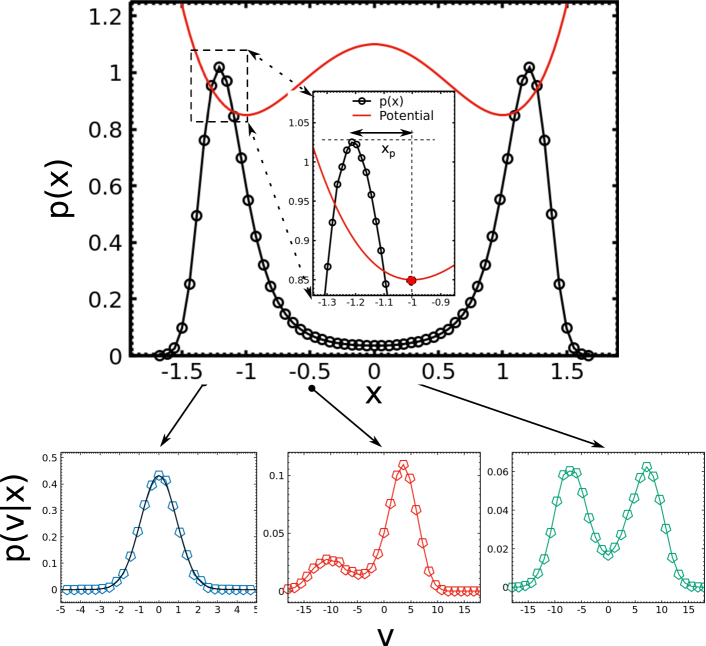
Figure 1: Upper panel: The marginal distribution $\rho(x)$ (black data) obtained from the numerical data and the double well potential (the red curve, rescaled for presentation reasons) for the parameter choice $a=b=10$ and. In the inset, we zoom the distribution near its left maximum. The variance of the self-propulsion force is $D_{a}/\tau=10^{2}$ and $\tau=10$. Notice that the positions of the peaks of the density $\rho(x)$ are slightly shifted with respect to the minima of the double well potential (11) and correspond fairly well to the roots of (14). Lower panel: we display the conditional velocity distribution, $p(v|x)$, for three different positions, $x=-1.2,-0.5,0.$ from the left to the right, respectively. In the vicinity of the two peaks of $\rho(x)$ at $x=\pm 1.2$ the distribution is unimodal $p(v|x)$. At $x=\pm 0.5$ a lateral shoulder appears as a clear indication of the onset of bimodality in the velocity distribution. Finally, at the symmetric point $x=0$ the bimodality of $p(v|x)$ is fully developed and the particles form two distinguishable populations: one of particles propagating towards the right and the other towards the left.

Figure 2: We show the snapshots representing the phase-points in the $(x,v)$-plane for two different choices of the persistence time $\tau$: left panel $\tau=1$ and right panel $\tau=10$. The remaining parameters are $D_{a}/\tau=10^{2}$ and $a=b=10$. Each point represents the state of one system at a given instant. We simulated a collection of $N=10^{3}$ particles. The vertical dashed curves are only a guide to the eye.

As we said above, the overall structure of $\rho(x)$ is not too dissimilar from the one one would observe in a thermal system, but if we scrutinize the system using a different indicator, i.e. the conditional probability of the system’s “velocity”, $p(v|x)=p(x,v)/\rho(x)$, the peculiarity of the active system becomes evident. In the bottom panels of Fig. 1 we plot the numerical data representing the conditional probability of the system’s “velocity”, $p(v|x)$ for three different typical positions, $x$: at the $\rho$-peak position, at the position of the maximum of the potential and at the intermediate point between them (left,right and middle panel, respectively). In the bottom left panel of Fig. 1, the conditional velocity distribution displays a single peak: such a form is consistent with the distribution Eq. (6) and corresponds with the existence of a positive local kinetic temperature which is well reproduced by $\theta(x)$ given by (10). We classify such a behavior as equilibrium-like and dub these regions of phase-space as ER. We define as ”non-equilibrium regions” (NER) the zones which are not ER. In particular, the NTR defined above is contained in the NER, since the study of the $p(v|x)$ shows clear non-equilibrium features. Indeed, for those values of $x$ where $\Gamma(x)$ becomes negative, the observed scenario is now more intriguing because the conditional distribution $p(v|x)$ displays bimodality: in the bottom center panel for $x=-0.5$ the main peak is shifted from $v=0$ to a positive value $v\approx 5$ and is accompanied by the emergence of a second lower peak centered at negative $v\approx-10$ (and vice-versa on the other side). Such an unbalanced shape of the $p(v|x)$ distribution disappears for $x=0$ where the two peaks are symmetric ( see bottom right panel). The $p(v|x)$ shown in the central and right panels is not consistent with Eq. (6) and cannot be accounted for by a Maxwell-type distribution.

In the two panels of Fig. 2, we display two phase-space snapshot configurations in the plane $(x,v)$ for two different choices of $\tau$ ($\tau=1,10$). In order to sample configurations corresponding to the same strength of the active force we used the same ratio $D_{a}/\tau=10^{2}$. Both snapshots reveal an interesting phenomenology which confirms the previous observations and helps us to gain some insight: particles spend most of their life in the equilibrium-like regions, but sometimes visit the NTR region. When this occurs, the particles experience an acceleration, due to the negative mobility $1/\Gamma(x)<0$, towards the opposite ER region. Finally, when the particles have crossed the NTR and reached the opposite side $\Gamma(x)$ returns to positive values and the motion becomes damped again with a concomitant restoring of the local Gaussian velocity distribution.

The $(x,v)$ scatter plot reveals the presence of two lanes (one in the in the upper half-plane and the other in the lower half) of representative points in the NTR connecting the two darker regions. If $\tau$ increases the two lanes become thinner along the $v$ direction as clearly shown in the right panel of Fig. 2. Let us also remark that a larger value of the persistence time, $\tau$, determines a stronger selection mechanism of the velocities of the particles which succesfully escape from one well to the other.

Such a picture is also confirmed by Fig. 3 where we report the values $v(t)$ and $x(t)$ for a single particle trajectory: in correspondence of the instant when the particle changes well, its velocity rapidly grows, a scenario which has not a Brownian analog and is peculiar of the active dynamics. In particular, $v(t)$ reveals pronounced spikes at the crossing barrier time, whose height are consistently larger that the typical equilibrium-like fluctuation, predicted by UCNA. The shape of the spikes resembles a deterministic trajectory and thus does not seem particularly affected by the random force, as shown in the Inset of Fig. 3.

Figure 3: In the upper left and right panel we show the evolution of the position, $x(t)$ for $\tau=1$ and $\tau=10$, respectively. In the lower panels, we display the corresponding velocities. The values of the remaining parameters are: $D_{a}/\tau=10^{2}$ and $a=b=10$.

Summarizing, we have found regions characterized by “local” negative temperatures: when a particle enters one of these regions, it becomes too energetic to remain there and thus has to leave it to enter again an ER, where $\Gamma(x)$ becomes again positive. This feed-back mechanism explains why the mean velocity does not grow indefinitely.

IV Analysis of the Negative Temperature Region

As shown in Figs. 1 and 2, an active particle spends the most of its life in the regions where the potential $U(x)$ is convex. Under such condition, the UCNA approach is expected to work and this fact is confirmed by the observation that the numerical $p(v|x)$ is well reproduced by a Gaussian with temperature $\theta(x)$ given by Eq. (10). However, this approximation is not uniformly valid in space as the presence of two peaks in $p(v|x)$ of Fig. 1 and the form of the snapshots of Fig. 2 have shown. To remedy this situation, in the present Section we attempt to formulate in alternative to the UCNA a theoretical explanation of the observed behavior in the region $(-x_{N},x_{N})$ i.e. where $\Gamma(x)<0$.

Hereafter, we propose a theoretical interpretation of the numerical findings illustrated above and is based on the analysis of the behavior of the slow variables of the system in this unstable region. We choose as slow variables the average velocity of the particles and velocity variance at fixed $x$ ( i.e. conditional averages) and determine their evolution. Since in the stationarity state the average velocity at a fixed arbitrary position vanishes, i.e. $\langle v(x)\rangle={\int dvvp(x,v)}/{\int dvp(x,v)}=0$, it is crucial to study separately the population of the particles going from the left well to the right one (the upper lane in Fig. 2), from those performing the opposite path.

To identify these two populations we define $p_{+}(x,v)$ ($p_{-}(x,v)$) as the unnormalized PDF of the particles whose dynamics starts from the left (right) well. In practice, we compute $p_{\pm}$ counting the particles in the two lanes of Fig. 2 and normalizing them with the total number of particles. In this way, summing over the two populations we recover the total distribution:

$$p(x,v)=p_{+}(x,v)+p_{-}(x,v).$$

The functional form of $p_{\pm}$ in the NTR will be investigated in the present section. Accordingly, we define the first conditional velocity moment with respect to $p_{\pm}(x,v)$:

$$\langle v(x)\rangle_{\pm}=\frac{\int p_{\pm}(x,v)vdv}{\int p_{\pm}(x,v)dv}.$$

Now, averaging Eq. (4) with respect to $p_{\pm}(x,v)/\int dvp_{\pm}(x,v)$ we obtain:

$$\frac{d}{dt}\langle v(x)\rangle_{\pm}=-\frac{1}{\tau}\left(1+\frac{\tau}{\gamma}U^{\prime\prime}(x)\right)\langle v(x)\rangle_{\pm}-\frac{U^{\prime}(x)}{\gamma\tau}.$$ (15)

In the region, where $\Gamma(x)<0$, the absolute value of the average $\langle v(x)\rangle_{\pm}$ grows exponentially in time before dropping to zero again, as one can observe qualitatively the inset of top-right panel of Fig. 3. In order to determine $\langle v(x)\rangle_{\pm}$, we specialize the treatment to the regime $\gamma\tau\gg 1$, where some approximations are possible and we can neglect the last term in the right hand side of the Eq. (15). This regime is the most interesting for the present study, since it is just the activity dominated regime. The integration of equation (15) is performed taking into account that the conditional averages $\langle v(x)\rangle_{\pm}$ are explicit functions of $x$ and $t$ so that the operator $d/dt$ is the total derivative:

$$d/dt=\partial_{t}+v\partial_{x}\approx\partial_{t}+\langle v(x)\rangle_{\pm}\partial_{x}\,.$$

We integrate Eq. (15) and obtain:

$$\langle v(x)\rangle_{\pm}=\langle v(x_{0})\rangle_{\pm}-\frac{U^{\prime}(x)}{\gamma}+\frac{U^{\prime}(x_{0})}{\gamma}+O\left(\frac{1}{\tau}\right)$$ (16)

where the lower limit of integration $x_{0}$ is given by $-x_{N}$ if the initial configuration starts in the left sector and the particle propagates from the left towards the right, while we choose $x_{0}=x_{N}$ in the opposite case. Such an equation expresses the conservation of the average self-propulsion, since $\langle f_{a}(x_{\pm})\rangle=\gamma\langle v(x)\rangle_{\pm}+U^{\prime}(x)=\pm const$ for $x\in(-x_{N},x_{N})$. Since we are considering $\tau\gg 1$ the microswimmers able to reach the NTR, are the fraction of particles with self-propulsion, $f_{a}$, large enough to reach the point $x_{0}$, as discussed in Section III. Moreover, until this fraction of particles reaches the opposite well, their self-propulsion will maintain a nearly constant value.

Let us, now, consider the equation of evolution for the slow variable $\langle v^{2}(x)\rangle_{\pm}$. To this purpose, we multiply by $v$ Eq. (4) and apply the Ito calculus Gardiner (2009) and obtain:

$$vdv=-\frac{\Gamma(x)}{\tau}v^{2}dt+v\frac{\sqrt{2D_{a}}}{\tau}\,dw-v\frac{U^{\prime}(x)}{\tau\gamma}dt$$ (17)

where $dw$ is the Wiener process associated with the white noise, $\eta$. By taking the average, $\langle\cdot\rangle_{\pm}$, we write an equation for $\langle v^{2}(x)\rangle_{\pm}$, which depends on $\langle v(x)\rangle_{\pm}$:

$$\frac{d}{dt}\langle v^{2}(x)\rangle_{\pm}=\langle v(x)\rangle_{\pm}\frac{d\langle v^{2}(x)\rangle_{\pm}}{dx}=-2\frac{\Gamma(x)}{\tau}\langle v^{2}(x)\rangle_{\pm}-2\langle v(x)\rangle_{\pm}\frac{U^{\prime}(x)}{\tau\gamma}+2\frac{D_{a}}{\tau^{2}}$$ (18)

where again in the first equality $d/dt$ is the total derivative. Such an equation, in the case of vanishing currents ($\langle v(x)\rangle_{\pm}=0$) and positive temperature, is in agreement with the UCNA prediction because we have the simple result: $\langle v^{2}(x)\rangle_{\pm}=\frac{D_{a}}{\tau\Gamma(x)},$ which is nothing but formula (10). In the more interesting case of non vanishing currents, Eq. (18) is an inhomogeneous first order differential equation for the observables $\langle v^{2}(x)\rangle_{\pm}$ and can be integrated through the formula

$$\langle v^{2}(x)\rangle_{\pm} =\langle v^{2}(x_{0})\rangle_{\pm}e^{-\int^{x}_{x_{0}}dx^{\prime}g(x^{\prime})}$$ (19)

$$+e^{-\int^{x}_{x_{0}}dx^{\prime}g(x^{\prime})}\int^{x}_{x_{0}}dx^{\prime}T(x^{\prime})e^{\int^{x^{\prime}}_{x_{0}}dx^{\prime\prime}g(x^{\prime\prime})}$$

where $g(x)=2\frac{\Gamma(x)}{\tau\langle v(x)\rangle_{\pm}}$, $T(x)=\frac{2D_{a}}{\tau^{2}\langle v(x)\rangle_{\pm}}$, and the term $\frac{U^{\prime}(x)}{\tau\gamma}=O(1/\tau)$ and has been neglected. In the limit $\tau\gg 1$, we obtain:

$$\int dxg(x)=\int dx\frac{2\Gamma(x)}{\left(\tau\langle v(x)\rangle_{\pm}\right)}\approx-2\ln{\langle v(x)\rangle_{\pm}}+O(1/\tau)$$ (20)

so that the solution of the inhomogeneous first order ordinary differential equation(18), simply reads:

$$\langle v^{2}(x)\rangle_{\pm}\approx\langle v^{2}(x_{0})\rangle_{\pm}\left(\frac{\langle v(x)\rangle_{\pm}}{\langle v(x_{0})\rangle_{\pm}}\right)^{2}+\left(\langle v(x)\rangle_{\pm}\right)^{2}\int^{x}_{x_{0}}dx^{\prime}\frac{2D_{a}}{\tau^{2}\left(\langle v(x^{\prime})\rangle_{\pm}\right)^{3}}.$$ (21)

Finally, since the last term in the the right hand side of Eq. (21) is negligible, being $O(D_{a}/\tau^{2})$ the variances $\Delta_{\pm}(x)\equiv\langle(v-\langle v(x)\rangle_{\pm})^{2}\rangle_{\pm}$ can be approximated as:

$$\Delta_{\pm}(x)\approx\left(\langle v(x)\rangle_{\pm}\right)^{2}\frac{\Delta_{\pm}(x_{0})}{\left(\langle v(x_{0})\rangle_{\pm}\right)^{2}}.$$ (22)

Eq. (22) establishes a simple approximate relation between the variances, $\Delta_{\pm}(x)$, and the first conditional velocity moments, $\langle v(x)\rangle_{\pm}$, which holds in the regime $\tau\gg 1$. We can roughly estimate the velocity variance at $x_{0}$ as $\Delta_{\pm}(x_{0})\approx D_{a}/(\tau\Gamma(x_{0}))\sim D_{a}/(\tau^{2}U^{\prime\prime}(x_{0}))$ and explain why at fixed $D_{a}/\tau$ the lanes in the scatter plot of Fig. 2 become thinner as $\tau$ increases.

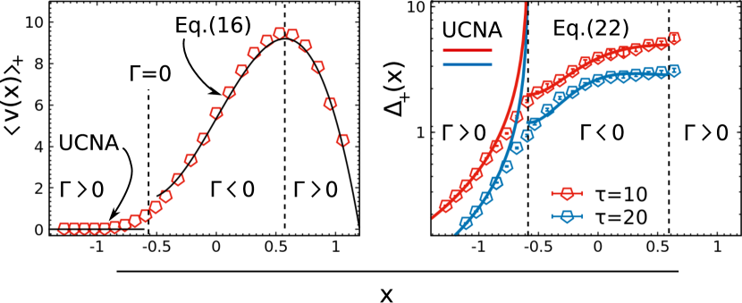
Figure 4: Left Panel: $\langle v(x)\rangle_{+}$ computed from data (red points) and from the theoretical prediction (black line) of Eq. (16) with the initial value, $\langle v(x_{0})\rangle_{+}=1.5$, obtained from the numerical data values data in correspondence of $\tau=10$. Right Panel: Variance $\Delta_{+}(x)$ computed from data (points) and from the theoretical prediction, respectively: in the left sector ($\Gamma>0$) the continuous lines represent the UCNA theoretical value for $\tau=10$ and $20$. In the central region ($\Gamma<0$) the continuous lines represent the prediction of Eq. (22) . The remaining parameters are $D_{a}/\tau=10^{2}$, $a=b=10$.

Let us consider now the phase-space distribution, $p(x,v)$ in the central region: using the above results we see that it can be approximated as the sum of two Gaussians, representing, respectively, the left and the right population:

$$p(x,v)\approx\mathcal{N}\left(\rho_{+}(x)\sqrt{\frac{1}{2\pi\Delta_{+}(x)}}\exp\left(-\frac{\left(v-\langle v(x)\rangle_{+}\right)^{2}}{2\Delta_{+}(x)}\right)+\rho_{-}(x)\sqrt{\frac{1}{2\pi\Delta_{-}(x)}}\exp\left(-\frac{\left(v-\langle v(x)\rangle_{-}\right)^{2}}{2\Delta_{-}(x)}\right)\right)$$ (23)

being $\mathcal{N}$ the normalization of the whole distribution. The form of (23) reproduces the structures observed in the lower panels of Fig. 1 and clearly, the presence of the double peak in the velocity distribution is the signature of a departure from the global equilibrium condition.

The theoretical predictions for $\langle v(x)\rangle_{\pm}$ and $\langle v^{2}(x)\rangle_{\pm}$ are tested against the respective numerical measures as shown in the left and right panel of Fig. 4, respectively. In particular, the study of $\langle v(x)\rangle_{+}$ obtained from data with the prediction (16) displays a good agreement in the NTR region, which confirms the present theory. Notice that Eq. (16) does not hold in the region where $\Gamma(x)>0$ and $\langle v(x)\rangle_{\pm}\approx 0$, which is instead well described by the UCNA approximation.

The variance of the left population, $\Delta(x)_{+}=\langle v^{2}(x)\rangle_{+}-\left[\langle v(x)\rangle_{+}\right]^{2}$, shown in the right panel of Fig. (4), increases monotonically with $x$. In particular, the variance reveals a good agreement with the UCNA prediction in the regions where $\Gamma(x)>0$. As $x$ tends from the left to $-x_{N}$, the space point where $\Gamma(x)=0$, the variance calculated with the UCNA diverges, in clear disagreement with the numerical findings of Fig. 4. However, if we consider the NTR region the agreement between data and the theoretical Eq. (22) is pretty good, confirming the validity of the approach.

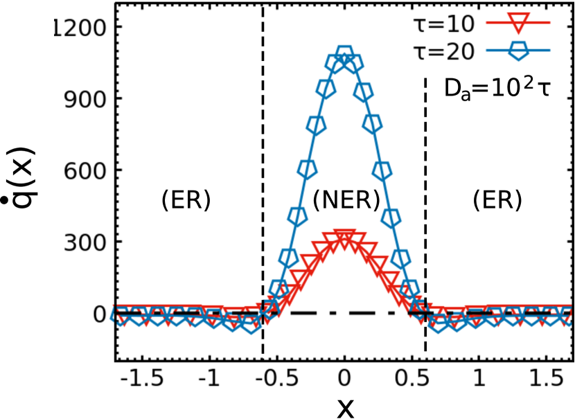
Figure 5: Plot of the heat flux, $\dot{q}$, defined by Eq.  (24) as a function of the position for two different values of $\tau=10,20$ and $D_{a}/\tau=10^{2}$. Notice that $\dot{q}$ is quite small and negative in the equilibrium-like region and large and positive in the negative temperature region. The main contribution to the entropy production stems from the equilibrium like region because the majority of the particles sit there. The remaining parameters are $a=b=10$.

V Energetics

We conclude with a brief discussion of the energetics of the model. Following the methods of Ref. Marconi, Puglisi, and Maggi (2017) we define the local heat flux, $\dot{q}(x,t)$, as the energy flux transferred from the active bath (represented by the Gaussian colored noise) to the particles. There it was shown, that such a flux can be expressed as:

$$\dot{q}(x,t)=-\frac{\Gamma(x)}{\tau\rho(x,t)}\int dv\Bigl{[}\tau\gamma v^{2}p(x,v,t)+\theta(x)v\frac{\partial}{\partial v}p(x,v,t)\Bigr{]}=-\frac{1}{\tau}\frac{D_{a}\gamma}{\theta(x)}\left[\tau\gamma\langle v^{2}(x)\rangle-\theta(x)\right].$$ (24)

and that the entropy production towards the surrounding medium reads:

$$\dot{s}_{m}(x,t)=\frac{\dot{q}(x,t)}{\theta(x)}.$$ (25)

It was also demonstrated that the total entropy production of the medium $\dot{S}_{m}(t)=\int dx\rho(x,t)\dot{s}_{m}(x,t)$ and the total heat flux are related through a generalised Clausius inequality Marconi, Puglisi, and Maggi (2017)

$$\dot{S}_{m}(t)=\int dx\rho(x,t)\frac{1}{\theta(x)}\dot{q}(x,t)\leq 0.$$ (26)

Such an expression for the entropy production of the AOUP is consistent with the results of Refs. Fodor et al. (2016); Puglisi and Marini Bettolo Marconi (2017); Dabelow, Bo, and Eichhorn (2018); Caprini et al. (2018).

Let us discuss the behavior of $\dot{q}(x,t)$ in the steady state, as shown in Fig. 5. We can identify two symmetric space regions, occurring at $\Gamma(x)>0$, where $\dot{q}(x)$ (or equivalently $\dot{s}_{m}(x)$) is almost zero. These zones coincide with the ”equilibrium-like regions” (ER) defined in Sec. III, a nomenclature which is well justified also from a stochastic thermodynamic approach. To be precise, in this region $\dot{q}(x)$ is not exactly zero but assumes very small negative values because in the last equality of Eq. (24) we have $\langle v^{2}(x)\rangle\geq\theta(x)/\tau\gamma$ and thus the contribution to $\dot{S}_{m}$ is negative. On the other hands, we call ”non-equilibrium space region” (NER) those zones where $\dot{q}(x)$ is large. In particular, the NTR region, introduced in Sec. III, is strictly contained in the NER, displaying large $\dot{q}(x)$, which assumes positive values. Indeed, both terms $-\theta(x)$ and $\langle v^{2}(x)\rangle$ contained in the last equality in Eq. (24) have the same positive sign. As shown in Fig. 5, $\dot{q}(x)$ grows as $\tau$ increases. Indeed, evaluating the regime $\tau\gg 1$ in Eq. (24) in the NTR, $\dot{q}(x)\approx-\Gamma(x)\langle v(x)\rangle\sim\tau|U^{\prime\prime}(x)|\langle v^{2}(x)\rangle$, showing the occurrence of an explicit $\tau$ dependence. Despite $\theta(x)$ approach to infinity for $\Gamma(x)=0$, in this special case $\dot{q}(x)$ is finite and positive and $\dot{s}_{m}(x)$ becomes zero. We outline that the correct sign of the inequality (26) is realized because $\rho(x)$ is very small in the NER and large in the ER.

Finally, we discuss the connection between the form of the distribution functions and the detailed balance condition. We have mentioned that in order to derive the UCNA steady state distribution one has to assume the vanishing of all currents, which is a form to say that the detailed balance condition holds. However, considering the AOUP one sees that the detailed balance condition holds and the entropy production vanishes only in the case of linear or quadratic potentials. For more general potentials the DB does not hold. Now, we argue that in the ER the local entropy production (25) is nearly vanishing, while in the NER (and in particular in the NTR) the local entropy production is large. In the first case a local version of the detailed balance appears to be satisfied whereas in the second case it is strongly violated. This picture is consistent with the Fig. 1: the Gaussian form of the $p(v|v)$ distribution shown in panel (b) of Fig. 1 indicates that the detailed balance condition is satisfied locally in the ER, whereas in the NTR (panels (c) and (d)) the presence of two peaks clearly shows a breakdown of such a condition.

VI Conclusion

Some comments are in order: we have studied an active Ornstein-Uhlenbeck particle in the presence of a bistable potential and found that for sufficiently large values of the persistence time $\tau$ the space accessible to the particle can classified into regions where the sign of the friction function $\Gamma(x)$ is either positive or negative, that we named equilibrium-like regions (ER) and nonequilibrium regions (NER), respectively. In the ER, characterized by a small entropy production and by the absence of currents, the statistical properties of the system are captured fairly well by an extended UCNA approximation which predicts a steady state unimodal distribution function $p(x,v)$ of the Maxwell-Boltzmann type. On the contrary, the NER is characterized by the bimodality of the velocity distribution, by larger values of the entropy production and by a strong departure from the detailed balance condition. Our theory, which is valid in the limit of large $\tau$, succesfully explains the dependence of the local currents $\langle v(x)\rangle_{\pm}$ and velocity moment $\langle v^{2}(x)\rangle_{\pm}$ on the control parameters.

We envisage an interesting application of our study: by employing a non-convex potential we may find a velocity selection mechanism which allows us to produce particles with a particular velocity. The selection becomes more efficient as the persistence time at fixed propulsion speed increases. Moreover, this ”device” gives the possibility of producing active particles with a super speed, $|v_{s}|$, some order of magnitude larger than the typical velocity of particles in the potential-free region. Clearly, this effect could be amplified by choosing the potential in such a way that $\Gamma(x)$ becomes more negative. It is worth to mention the fact that the presence of negative mobility regions Eichhorn, Reimann, and Hänggi (2002) is even more severe in two and three dimensions where it naturally occurs for instance near a concave surface Fily, Baskaran, and Hagan (2017). In this case, the mobility is a tensor and its tangential components may become negative when the curvature radius is small. Another important issue is the case where the particles are mutually interacting via some pair potential: the mobility matrix even for small persistence can display negative eigenvalues in such a way that the UCNA is not applicable in all regions. It would be interesting to explore if these multidimensional cases could be treated using concepts similar to those exploited in the present work.