Scattering of Spinning Black Holes from Exponentiated Soft Factors

Abstract

We provide evidence that the classical scattering of two spinning black holes is controlled by the soft expansion of exchanged gravitons. We show how an exponentiation of Cachazo-Strominger soft factors, acting on massive higher-spin amplitudes, can be used to find spin contributions to the aligned-spin scattering angle, conjecturally extending previously known results to higher orders in spin at one-loop order. The extraction of the classical limit is accomplished via the on-shell leading-singularity method and using massive spinor-helicity variables. The three-point amplitude for arbitrary-spin massive particles minimally coupled to gravity is expressed in an exponential form, and in the infinite-spin limit it matches the effective stress-energy tensor of the linearized Kerr solution. A four-point gravitational Compton amplitude is obtained from an extrapolated soft theorem, equivalent to gluing two exponential three-point amplitudes, and becomes itself an exponential operator. The construction uses these amplitudes to: 1) recover the known tree-level scattering angle at all orders in spin, 2) recover the known one-loop linear-in-spin interaction, 3) match a previous conjectural expression for the one-loop scattering angle at quadratic order in spin, 4) propose new one-loop results through quartic order in spin. These connections link the computation of higher-multipole interactions to the study of deeper orders in the soft expansion.

1 Introduction

In 2014 Cachazo and Strominger Cachazo:2014fwa showed that the soft limit of tree-level gravity amplitudes is controlled by the action of the angular momentum operator $J^{\mu\nu}$, i.e.

$${\cal M}_{n+1}=\sum_{i=1}^{n}\left[\frac{(p_{i}\cdot\varepsilon)^{2}}{p_{i}\cdot k}+i\frac{(p_{i}\cdot\varepsilon)(k_{\mu}\varepsilon_{\nu}J_{i}^{\mu\nu})}{p_{i}\cdot k}-\frac{1}{2}\frac{(k_{\mu}\varepsilon_{\nu}J_{i}^{\mu\nu})^{2}}{p_{i}\cdot k}\right]{\cal M}_{n}+{\cal O}(k^{2}),$$ (1)

up to sub-subleading order. Here the soft momentum $k$ corresponds to the external soft graviton, and we have constructed its polarization tensor as $\varepsilon_{\mu\nu}=\varepsilon_{\mu}\varepsilon_{\nu}$. The sum is over the remaining external particles with momenta $p_{i}^{\mu}$, and the operators $J_{i}^{\mu\nu}$ acting on them include both orbital and spin parts of the angular momentum. The first term is simply the standard Weinberg soft factor Weinberg:1965nx , whose universality is associated to the equivalence principle. Following the QED results of Low Low:1954kd ; Low:1958sn , the subleading behaviour of gravity amplitudes was first studied long ago by Gross and Jackiw Gross:1968in ; Jackiw:1968zza . Indeed, it was already observed in Gross:1968in ; Jackiw:1968zza that the subleading soft theorem follows from gauge invariance (see White:2011yy ; Bern:2014vva for a modern perspective), and because of this, it also adopts a universal form up to subleading order. Starting at sub-subleading order the soft expansion can depend on the matter content and EFT operators present in the theory Laddha:2017ygw ; Sen:2017xjn ; Bianchi:2014gla , although it is known that gauge invariance still provides partial information at all orders Hamada:2018vrw ; Li:2018gnc . On a different front, the realization that soft theorems correspond to Ward identities for asymptotic symmetries at null infinity Strominger:2013jfa has led to impressive and wide-reaching developments He:2014laa ; Cachazo:2014fwa ; Cachazo:2014dia ; Kapec:2014opa ; Bern:2014vva ; Dumitrescu:2015fej ; Campiglia:2016hvg , see Strominger:2017zoo for a recent review. Following such correspondence, an infinite tower of Ward identities has indeed been proposed to follow from all orders in the soft expansion Campiglia:2018dyi .

Recently, a classical version of the soft theorem up to sub-subleading order has been used by Laddha and Sen Laddha:2018rle to derive the spectrum of the radiated power in black-hole scattering with external soft graviton insertions. This relies on the remarkable fact that conservative and non-conservative long-range effects of interacting black holes can be computed from the scattering of massive point-like sources Duff:1973zz ; BjerrumBohr:2002ks ; Neill:2013wsa ; Bjerrum-Bohr:2018xdl . Indeed, rotating black holes can be treated via a spin-multipole expansion, the order $2s$ of which can be reproduced by scattering spin-$s$ minimally coupled particles exchanging gravitons Vaidya:2014kza , as illustrated in figure 1(a). The matching between these amplitudes with spin and a non-relativistic potential for black-hole scattering has been performed explicitly in the post-Newtonian (PN) framework Vaidya:2014kza ; Holstein:2008sx ; Guevara:2017csg .

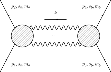
(a)

(b)

Figure 1: (a) Four-point amplitude involving the exchange of soft gravitons, which leads to classical observables. The external massive states are interpreted as two black-hole sources.
(b) Comparison between the HCL and the non-relativistic limit in the COM frame Holstein:2008sx ; Holstein:2008sw ; Vaidya:2014kza . Spin effects require subleading orders in the nonrelativistic (NR) classical limit, but can be fully determined at the leading order in HCL through the soft expansion.

Here we present a complementary picture to the one of Laddha:2018rle by employing the soft theorem in the conservative sector (i.e. no external gravitons), focusing on rotating black holes and at the same time extending the soft factor in (1) to higher orders in the soft expansion. This is achieved in the following way: It was shown by one of the authors in Guevara:2017csg that the classical ($\hbar$-independent) piece of the spin-$s$ amplitude can be extracted from a covariant Holomorphic Classical Limit (HCL), which sets the external kinematics such that the momentum transfer $k$ between the massive sources is null. On the support of the leading-singularity (LS) construction Cachazo:2017jef , which drops $\mathcal{O}(\hbar)$ parts, the condition $k^{2}=0$ reduces the amplitude to a purely classical expansion in spin multipoles of the form $\sim k^{n}S^{n}$, where $S$ carries the intrinsic angular momentum of the black hole (see figure 1(b)). This precisely matches the soft expansion once the momentum transfer is recognized as the graviton momentum and the classical spin vector $S$ is identified with the angular momentum $J_{i}$ of the matter particles.

To see the soft expansion more explicitly, consider the energy-momentum tensor of a single linearized Kerr black hole, which has recently been written down in an exponential form by one of the authors Vines:2017hyw :

$$T^{\mu\nu}(-k)=2\pi\delta{(p\cdot k)}p^{(\mu}\exp(a*ik)^{\nu)}{}_{\rho}\;\!p^{\rho}+\mathcal{O}(G),$$ (2)

where $(a*k)^{\mu}{}_{\nu}=\epsilon^{\mu}{}_{\nu\rho\sigma}a^{\rho}k^{\sigma}$, and $a^{\mu}={S^{\mu}}/{m}$ is the rescaled spin vector of the black hole. The magnitude $a$ is exactly the radius of its ring singularity. Here we have performed a Fourier transform of the worldline formulas (18) and (32a) of Vines:2017hyw . Now, the interaction vertex between a graviton and a massive source corresponds to the contraction $-h_{\mu\nu}T^{\mu\nu}$. After we take the graviton to be on-shell and replace $h_{\mu\nu}(k)$ by $2\pi\delta{(k^{2})}\varepsilon_{\mu}\varepsilon_{\nu}$, the vertex becomes

$$h_{\mu\nu}(k)T^{\mu\nu}(-k)=(2\pi)^{2}\delta{(k^{2})}\delta{(p\cdot k)}(p\cdot\varepsilon)\;\!\varepsilon_{\mu}p_{\nu}\bigg{[}\eta^{\mu\nu}-i\epsilon^{\mu\nu\rho\sigma}k_{\rho}a_{\sigma}+\frac{1}{2}\eta^{\mu\nu}(a\cdot k)^{2}+\mathcal{O}(k^{3})\bigg{]},$$ (3)

where we have used the support of the delta functions. This expression can be written in a simple form by introducing the spin tensor

$$S^{\mu\nu}=\epsilon^{\mu\nu\rho\sigma}p_{\rho}a_{\sigma}\qquad\Rightarrow\qquad a_{\lambda}=\frac{1}{2m^{2}}\epsilon_{\lambda\mu\nu\rho}S^{\mu\nu}p^{\rho},$$ (4)

satisfying $S^{\mu\nu}p_{\nu}=0$, after which it becomes

$$h_{\mu\nu}(k)T^{\mu\nu}(-k) =(2\pi)^{2}\delta{(k^{2})}\delta{(p\cdot k)}(p\cdot\varepsilon)^{2}\exp\!\bigg{(}\!{-i}\frac{k_{\mu}\varepsilon_{\nu}S^{\mu\nu}}{p\cdot\varepsilon}\bigg{)}$$ (5)

$$=(2\pi)^{2}\delta{(k^{2})}\delta{(p\cdot k)}(p\cdot\varepsilon)^{2}\Bigg{[}1-i\frac{k_{\mu}\varepsilon_{\nu}S^{\mu\nu}}{p\cdot\varepsilon}-\frac{1}{2}\bigg{(}\frac{k_{\mu}\varepsilon_{\nu}S^{\mu\nu}}{p\cdot\varepsilon}\bigg{)}^{\!2}+{\cal O}(k^{3})\Bigg{]}.$$

The terms inside the parentheses look precisely like an exponential completion of the expansion in eq. (1). Here it naturally appeared as a rewrite of the exponential structure of the linearized Kerr energy-momentum tensor. We will see that this structure extends way beyond what is guaranteed by universality and it is a consequence of the ‘minimally coupled’ nature of the Kerr solution. Note that the prefactor ${(p\cdot\varepsilon)^{2}}$ corresponds to the contribution of the energy-momentum tensor of the linearized Schwarzschild solution Damour:2016gwp .

Even though the fact that classical gravitational quantities can be reproduced from QFT computations has been known for a long time, the precise conceptual foundations of the matching are still lacking. The goal of one of the authors in Guevara:2017csg was simply to show the agreement of the LS method with the previous computations of Holstein:2008sw ; Holstein:2008sx ; Vaidya:2014kza . Moreover, in Guevara:2017csg the new massive spinor-helicity variables of Arkani-Hamed, Huang and Huang Arkani-Hamed:2017jhn were implemented to construct operators carrying spin multipoles. These operators were then matched, trough a change of basis, to those constructed in Holstein:2008sw ; Holstein:2008sx ; Vaidya:2014kza in terms of polarization vectors and Dirac spinors, enabling a systematic translation between the LS and the standard QFT amplitude in the $\hbar\to 0$ limit. It is only after computing the effective potential from this amplitude that one matches the post-Newtonian potential of general relativity.

The computation of the classical piece of the amplitude was made direct, through the leading singularity, for arbitrary spin and all orders in the center-of-mass energy $E$. Both the tree-level and one-loop versions of this computation correspond to a single order in the post-Minkowskian (PM) expansion (see e.g. recent discussion in Damour:2016gwp ; Bini:2017xzy ; Vines:2017hyw ; Damour:2017zjx ; Bini:2018ywr ; Bjerrum-Bohr:2018xdl ; Cheung:2018wkq ; Vines:2018gqi and many more references therein), i.e. at a fixed power of $G$. However, the explicit match to the standard QFT amplitude was only performed up to spin-1 and leading order in $E$ (which corresponds to the standard PN expansion). Moreover, the computation of the PN effective potential through the Born approximation suffers some complications Holstein:2008sx ; Neill:2013wsa . Such potential is not gauge-invariant, i.e. not an observable, and can undergo canonical and non-canonical transformations that become cumbersome when spin is considered as part of the phase space. Moreover, at one loop the Born approximation itself requires the subtraction of tree-level pieces and suffers from some (apparent) inconsistencies already at spin-1 Holstein:2008sw . For these reasons a more direct conversion from the LS into a gravitational observable is evidently needed. Very recently, a direct approach was proposed in the amplitudes setup to evaluate the scattering angle of classical general relativity Bjerrum-Bohr:2018xdl , i.e. the deflection angle of two massive particles in the large-impact-parameter regime. It was demonstrated that for scalar particles the scattering angle computed by Westphal Westpfahl:1985 can be obtained via a simple 2D Fourier transform of the classical limit of the amplitude.

Here we will show that the natural extension of the scattering angle, for aligned spins as in Bini:2017xzy ; Vines:2017hyw ; Bini:2018ywr ; Vines:2018gqi , can be computed with spinning particles directly from the LS. The building blocks needed for this computation are the three-point amplitude and the Compton amplitude for massive spinning particles interacting with soft gravitons. We will use the soft expansion with respect to the internal gravitons to write the building blocks in an exponentiated form, which fits naturally into the Fourier transform leading to the first and second post-Minkowskian (1PM and 2PM) scattering angles in a resummed form.

Summary of Results

In section 2.2 we show that the three-point scattering amplitude between two massive particles of spin $s$ and one graviton is given by

$${\cal M}_{3}^{(s)}(p_{1},p_{2},k^{-})=\left(-\frac{\kappa}{2}\right)\times\frac{2(p\cdot\varepsilon)^{2}}{m^{2s}}\,\langle 2|^{2s}\exp\!\bigg{(}i\frac{k_{\mu}\varepsilon_{\nu}J^{\mu\nu}}{p\cdot\varepsilon}\bigg{)}|1\rangle^{2s},\qquad\quad p=\frac{p_{1}-p_{2}}{2},$$ (6)

where the exponential operator is generated by the angular momentum $J^{\mu\nu}$, as appearing in the soft theorem (1). This operator acts naturally on the product states $|1\rangle^{2s}$ or $|2\rangle^{2s}$, which are constructed from the new spinor-helicity variables introduced by Arkani-Hamed, Huang and Huang Arkani-Hamed:2017jhn . Denoting the operator by $\hat{\cal M}_{3}^{(s)}$ we write this as

$$\hat{\cal M}_{3}^{(s)}={\cal M}_{3}^{(0)}\exp\!\bigg{(}i\frac{k_{\mu}\varepsilon_{\nu}J^{\mu\nu}}{p\cdot\varepsilon}\bigg{)},$$ (7)

where ${\cal M}_{3}^{(0)}$ corresponds to the amplitude for a massive scalar emitting a graviton. In section 2.3 we extend this result to the distinct-helicity Compton amplitude, showing that

$${\cal M}_{4}^{(s)}(p_{1},p_{2},k_{3}^{+},k_{4}^{-})=\frac{1}{m^{2s}}\langle 2|^{2s}\hat{\cal M}_{4}^{(s)}|1\rangle^{2s},\qquad\quad\hat{\cal M}_{4}^{(s)}={\cal M}_{4}^{(0)}\exp\!\bigg{(}i\frac{k_{4\mu}\varepsilon_{4\nu}J^{\mu\nu}}{p\cdot\varepsilon_{4}}\bigg{)},$$ (8)

up to corrections of fifth order in $J$ (appearing only for $s>2$). In the operator form, $k_{4}$ and $\varepsilon_{4}$ can be replaced by $k_{3}$ and $\varepsilon_{3}$, which simply amounts to a change of basis. The soft theorem (1) in this case is extrapolated in an exponential form, and corresponds to the simple statement of factorization of the Compton amplitudes into three-point amplitudes given by eq. (7) and its plus-helicity version.

The formulas (7) and (8) are the two building blocks needed to compute the scattering angle. In order to recover the classical observables we introduce and compute the generalized expectation value (GEV)

$$\langle{\cal M}^{(s)}_{n}\rangle=\frac{\varepsilon_{2,\mu_{1}\ldots\mu_{s}}\hat{{\cal M}}^{\mu_{1}\ldots\mu_{s},\nu_{1}\ldots\nu_{s}}_{n}\varepsilon_{1,\nu_{1}\ldots\nu_{s}}}{\varepsilon_{2}^{\mu_{1}\ldots\mu_{s}}\varepsilon_{1,\mu_{1}\ldots\mu_{s}}}=\frac{{\cal M}^{(s)}_{n}}{\varepsilon_{2}^{\mu_{1}\ldots\mu_{s}}\varepsilon_{1,\mu_{1}\ldots\mu_{s}}}.$$ (9)

Here we focus on integer-spin particles for simplicity, therefore we use polarization tensors for spin $s$. We first show that, with $h_{\mu\nu}=2\pi\delta(k^{2})\varepsilon_{\mu}\varepsilon_{\nu}$,

$$h_{\mu\nu}(k)T^{\mu\nu}(-k)=\frac{1}{2}(2\pi)^{2}\delta(k^{2})\delta(p\cdot k)\lim_{s\rightarrow\infty}\langle{\cal M}^{(s)}_{3}\rangle\bigg{|}{\begin{subarray}{c}~{}\\ ~{}\\ p_{1}=\,p-k/2~{}\\ \>p_{2}=-p-k/2\end{subarray}},$$ (10)

where $T^{\mu\nu}$ on the LHS is the linearized stress-energy tensor of the Kerr black hole (5). We then construct the aligned-spin scattering angle, for two-spinning-black-hole scattering, as in Kabat:1992tb ; Akhoury:2013yua ; Bjerrum-Bohr:2018xdl ,

$$\theta=-\frac{E}{(2m_{a}m_{b}\gamma v)^{2}}\frac{\partial~{}}{\partial b}\int\!\frac{d^{2}\boldsymbol{k}}{(2\pi)^{2}}\,e^{i\boldsymbol{k}\cdot\boldsymbol{b}}\lim_{s_{a},s_{b}\to\infty}\langle{\cal M}_{4}^{(s_{a},s_{b})}\rangle+{\cal O}(G^{3})$$ (11)

(see section 3.2 for definitions). Here ${\cal M}_{4}^{(s_{a},s_{b})}$ corresponds to the four-point amplitude of figure 1(a), with masses $m_{a}$ and $m_{b}$ and spin quantum numbers $s_{a}$ and $s_{b}$. We compute this amplitude at both tree and one-loop levels using the LS proposed in Guevara:2017csg . The Fourier transform can be performed using the exponential forms (7)-(8).

We find the following expression for the aligned-spin scattering angle $\chi$ as a function of the masses $m_{a}$ and $m_{b}$, the rescaled spins (ring radii, intrinsic angular momenta per mass) $a_{a}$ and $a_{b}$, the relative velocity at infinity $v$, and the proper impact parameter $b$ (the impact parameter separating the zeroth-order/asymptotic worldlines defined by each black hole’s Tulczyjew spin supplementary condition Tulczyjew:1959 ):

$$\theta=\frac{GE}{v^{2}}\bigg{[}\frac{(1+v)^{2}}{b+a_{a}+a_{b}}+\frac{(1-v)^{2}}{b-a_{a}-a_{b}}\bigg{]}-\pi G^{2}E\,\frac{\partial~{}}{\partial b}\bigg{[}m_{b}f(a_{a},a_{b})+m_{a}f(a_{b},a_{a})\bigg{]}+{\cal O}(G^{3}),$$ (12a)

where $$E=\sqrt{m_{a}^{2}+m_{b}^{2}+2m_{a}m_{b}\gamma} \gamma=(1-v^{2})^{-1/2}$$ with , and

$$f(\sigma,a)=\frac{1}{2a^{2}}\left({-b}+\frac{(\jmath+\varkappa-2a)^{5}}{4v\varkappa\big{[}(\jmath+\varkappa)^{2}-(2va)^{2}\big{]}^{3/2}}\right)+{\cal O}(\sigma^{5}),$$ (12b)

with

$$\jmath=vb+\sigma+a,\qquad\quad\varkappa=\sqrt{\jmath^{2}-4va(b+v\sigma)}.$$ (12c)

This agrees with previous classical computations to all orders in spin at tree level (at linear order in $G$) Bini:2017xzy ; Vines:2017hyw and through linear order in spin at one loop (at order $G^{2}$) Bini:2018ywr , as well as with the conjectural one-loop quadratic-in-spin expression presented in Vines:2018gqi . Moreover, eq. (12) resums those contributions in a compact form, including higher orders in spin. We have indicated that the expression (12b) is valid up to quartic order in one of the spins (but to all orders in the other spin) according to the minimally coupled higher-spin amplitudes.

2 Multipole expansion of three- and four-point amplitudes

2.1 Massive spin-1 matter

We start our discussion of the multipole expansion by dissecting the case of graviton emission by two massive vector fields. The corresponding three-particle amplitude reads

$${\cal M}_{3}(p_{1},p_{2},k)=-2(p\cdot\varepsilon)\big{[}(p\cdot\varepsilon)(\varepsilon_{1}\!\cdot\varepsilon_{2})-2k_{\mu}\varepsilon_{\nu}\varepsilon_{1}^{[\mu}\varepsilon_{2}^{\nu]}\big{]},\qquad\quad p=\frac{1}{2}(p_{1}-p_{2}),$$ (13)

where $p$ is the average momentum of the spin-1 particle before and after the graviton emission and the polarization tensor of the graviton $\varepsilon_{\mu\nu}=\varepsilon_{\mu}\varepsilon_{\nu}$ (with momentum $k=-p_{1}-p_{2}$) is split into two massless polarization vectors. The derivation of eq. (13) from the Proca action is detailed in appendix A, which also motivates that the term involving $\varepsilon_{1}^{[\mu}\varepsilon_{2}^{\nu]}$ can be thought of as an angular-momentum contribution to the scattering. In other words, we are tempted to interpret the combination $\varepsilon_{1}^{[\mu}\varepsilon_{2}^{\nu]}$ as being (proportional to) the classical spin tensor.

However, we now face our first challenge: as explained in Holstein:2008sw ; Holstein:2008sx ; Vaidya:2014kza , the spin-1 amplitude contains up to quadrupole interactions, i.e. quadratic in spin, whereas only the linear piece is apparent in eq. (13). To rewrite this contribution in terms of multipoles, we can use a redefined spin tensor

$$S^{\mu\nu}=-\frac{i}{\varepsilon_{1}\!\cdot\varepsilon_{2}}\bigg{\{}2\varepsilon_{1}^{[\mu}\varepsilon_{2}^{\nu]}-\frac{1}{m^{2}}p^{[\mu}\big{(}(k\cdot\varepsilon_{2})\varepsilon_{1}+(k\cdot\varepsilon_{1})\varepsilon_{2}\big{)}^{\nu]}\bigg{\}}.$$ (14)

It is introduced in appendix B via a two-particle expectation value/matrix element, which we call the generalized expectation value (GEV)

$$S^{\mu\nu}=\frac{\varepsilon_{2\sigma}\hat{\Sigma}^{\mu\nu,\sigma}_{~{}~{}~{}~{}\;\tau}\varepsilon_{1}^{\tau}}{\varepsilon_{2\sigma}\varepsilon_{1}^{\sigma}}.$$ (15)

Here $\hat{\Sigma}^{\mu\nu}$ is constructed as an angular-momentum operator shifted in such a way that its GEV satisfies the Fokker-Tulczyjew covariant spin supplementary condition (SSC) Fokker:1929 ; Tulczyjew:1959

$$p_{\mu}S^{\mu\nu}=0.$$ (16)

In this paper we find this condition to be crucial for the matching to the rotating-black-hole computation of Vines:2017hyw , as the classical spin tensor $S^{\mu\nu}$ (4) satisfies the above SSC by definition. The purpose of this SSC is to constrain the mass-dipole components $S^{0i}$ of the spin tensor of an object to vanish in its rest frame. In a classical setting it puts the reference point for the intrinsic spin of a spatially extended object at its rest-frame center of mass.

Inserting this spin tensor in eq. (17), we rewrite the above amplitude as

$${\cal M}_{3}(p_{1},p_{2},k) =-m^{2}x^{2}(\varepsilon_{1}\!\cdot\varepsilon_{2})\bigg{[}1-\frac{i\sqrt{2}}{mx}k_{\mu}\varepsilon_{\nu}S^{\mu\nu}+\frac{(k\cdot\varepsilon_{1})(k\cdot\varepsilon_{2})}{m^{2}(\varepsilon_{1}\!\cdot\varepsilon_{2})}\bigg{]},$$ (17)

where for further convenience we also expressed the scalar products $p\cdot\varepsilon$ using a helicity variable $x$ first introduced in ArkaniHamed:2008gz

$$x=\sqrt{2}\,\frac{p\cdot\varepsilon}{m}$$ (18)

(at higher points it becomes gauge-dependent but can still be used as a shorthand). Now, in the GEV of the amplitude,

$$\langle\mathcal{M}_{3}\rangle=\frac{\varepsilon_{2\sigma}\mathcal{M}_{3}^{\sigma\tau}\varepsilon_{1,\tau}}{\varepsilon_{2\sigma}\varepsilon_{1}^{\sigma}}=-m^{2}x^{2}\bigg{[}1-i\frac{k_{\mu}\varepsilon_{\nu}S^{\mu\nu}}{p\cdot\varepsilon}+\frac{(k\cdot\varepsilon_{1})(k\cdot\varepsilon_{2})}{m^{2}(\varepsilon_{1}\!\cdot\varepsilon_{2})}\bigg{]},$$ (19)

we recognize the dipole coupling of eq. (5) as the term linear in both $k$ and $S$. Indeed, particles with spin couple naturally to the field-strength tensor of the graviton $F_{\mu\nu}=2k_{[\mu}\varepsilon_{\nu]}$, analogously to the magnetic dipole moment $F_{\mu\nu}S^{\mu\nu}$. Following the non-relativistic limit, the third term was identified in Holstein:2008sw ; Holstein:2008sx ; Vaidya:2014kza ; Guevara:2017csg to be the quadrupole interaction $\propto\big{(}F_{\mu\nu}S^{\mu\nu}\big{)}^{2}$ for spin-1. It may seem a priori puzzling that we wish to regard the interaction $(k\cdot\varepsilon_{1})(k\cdot\varepsilon_{2})$ as the square of $F_{\mu\nu}S^{\mu\nu}$. This is because the statement is true at the levels of spin operators, but not at the level of (generalized) expectation values, i.e. $\langle F_{\mu\nu}\hat{\Sigma}^{\mu\nu}\rangle^{2}\neq\langle\big{(}F_{\mu\nu}\hat{\Sigma}^{\mu\nu}\big{)}^{2}\rangle$. In order to expose the exponential structure described in the introduction and construct such spin operators at any order, we are going to recast the multipole expansion in terms of spinor-helicity variables.

2.1.1 Spinor-helicity recap

This subsection can be skipped if the reader is familiar with the massive spinor-helicity formalism of Arkani-Hamed, Huang and Huang Arkani-Hamed:2017jhn , which is well suited to describe scattering amplitudes for massive particles with spin. Much like its massless counterpart, this formalism allows to construct all of the scattering kinematics from basic ${\rm SL}(2,\mathbb{C})$ spinors that transform covariantly with respect to the little group of the associated particle. The massive little group is ${\rm SU}(2)$, so the Pauli-matrix map from two-spinors to momenta

$$p_{\alpha\dot{\beta}}=p_{\mu}\sigma^{\mu}_{\alpha\dot{\beta}}=\epsilon_{ab}|p^{a}\rangle_{\alpha}[p^{b}|_{\dot{\beta}}=|p^{a}\rangle_{\alpha}[p_{a}|_{\dot{\beta}}=\lambda_{\alpha}^{~{}a}\tilde{\lambda}_{\dot{\beta}a},$$ (20)

involves a contraction of the ${\rm SU}(2)$ indices $a,b,\ldots=1,2$ (not to be confused with the spinorial ${\rm SL}(2,\mathbb{C})$ indices $\alpha,\beta,\ldots=1,2$ and $\dot{\alpha},\dot{\beta},\ldots=1,2$). This is in contrast to the massless case, where the little group is ${\rm U}(1)$, so its index is naturally hidden inside the complex nature of massless two-spinors

$$k_{\alpha\dot{\beta}}=k_{\mu}\sigma^{\mu}_{\alpha\dot{\beta}}=|k\rangle_{\alpha}[k|_{\dot{\beta}}=\lambda_{\alpha}\tilde{\lambda}_{\dot{\beta}}.$$ (21)

Now just as $\lambda_{\alpha}$ and $\tilde{\lambda}_{\dot{\beta}}$ are convenient to built massless polarization vectors (23), we can use the massive spinors $\lambda_{\alpha}^{~{}a}$ and $\tilde{\lambda}_{\dot{\beta}}^{~{}b}$ to construct spin-$S$ external wavefunctions. For instance, massive polarization vectors are explicitly

$$\varepsilon_{p\>\!\mu}^{ab}=\frac{\langle p^{(a}|\sigma_{\mu}|p^{b)}]}{\sqrt{2}m}\qquad\Rightarrow\qquad\left\{\begin{aligned} p\cdot\varepsilon_{p}^{ab}&=0,\\ \varepsilon_{p\>\!\mu}^{ab}\varepsilon_{p\>\!\nu ab}&=\eta_{\mu\nu}-\frac{p_{\mu}p_{\nu}}{m^{2}}\\ \varepsilon_{p\>\!11}\!\cdot\!\varepsilon_{p}^{11}&=\varepsilon_{p\>\!22}\!\cdot\!\varepsilon_{p}^{22}=2\>\!\varepsilon_{p\>\!12}\!\cdot\!\varepsilon_{p}^{12}=1,\end{aligned}\right.$$ (22)

where the symmetrized little-group indices $(ab)$ represent the physical spin-projection numbers $1,0,-1$ with respect to a spin quantization axis, as chosen by the massive spinor basis. Note that the vector indices, as well as their dotted and undotted spinorial counterparts, must always be contracted and do not represent a physical quantum number.

Let us also point out here that the massless polarization vectors and hence the associated helicity variable (18) can be written in terms of massless spinors as

$$\varepsilon_{+}^{\mu}=\frac{\langle r|\sigma^{\mu}|k]}{\sqrt{2}\langle r\;\!k\rangle},\qquad\quad\varepsilon_{-}^{\mu}=-\frac{[r|\bar{\sigma}^{\mu}|k\rangle}{\sqrt{2}[r\;\!k]}\qquad\Rightarrow\qquad x_{+}=\frac{\langle r|p|k]}{m\langle r\;\!k\rangle},\qquad x_{-}=-\frac{[r|p|k\rangle}{m[r\;\!k]}=-\frac{1}{x_{+}},$$ (23)

where $x$ is independent of the reference momentum $r$ on the three-point on-shell kinematics.

2.1.2 Spin-1 amplitude in spinor-helicity variables

We can now obtain concrete spinor-helicity expressions for the amplitude (13). Choosing the polarization of the graviton to be negative, we have

$$\varepsilon_{1}^{a_{1}a_{2}}\!\cdot\varepsilon_{2}^{b_{1}b_{2}} =-\frac{1}{m^{2}}\langle 1^{(a_{1}}2^{(b_{1}}\rangle\bigg{[}\langle 1^{a_{2})}2^{b_{2})}\rangle-\frac{1}{mx}\langle 1^{a_{2})}k\rangle\langle k\;\!2^{b_{2})}\rangle\bigg{]},$$ (24a)

$$\!\big{[}(\varepsilon_{1}\!\cdot\varepsilon_{2})k_{\mu}\varepsilon_{\nu}^{-}S^{\mu\nu}\big{]}^{a_{1}a_{2}b_{1}b_{2}} =\frac{i}{\sqrt{2}m^{2}}\langle 1^{(a_{1}}k\rangle\bigg{[}\langle 1^{a_{2})}2^{(b_{1}}\rangle-\frac{1}{2mx}\langle 1^{a_{2})}k\rangle\langle k\;\!2^{(b_{1}}\rangle\bigg{]}\langle k\;\!2^{b_{2})}\rangle,$$ (24b)

$$(k\cdot\varepsilon_{1}^{a_{1}a_{2}})(k\cdot\varepsilon_{2}^{b_{1}b_{2}}) =-\frac{1}{2m^{2}x^{2}}\langle 1^{(a_{1}}k\rangle\langle 1^{a_{2})}k\rangle\langle k\;\!2^{(b_{1}}\rangle\langle k\;\!2^{b_{2})}\rangle,$$ (24c)

where we have reduced all $[1^{a}|$ and $|2^{b}]$ to the chiral spinor basis of $\langle 1^{a}|$ and $|2^{b}\rangle$ using the following identities for the three-point kinematics,

$$[1^{a}k]=x^{-1}\langle 1^{a}k\rangle,\qquad\quad[2^{b}k]=-x^{-1}\langle 2^{b}k\rangle,\qquad\quad[1^{a}2^{b}]=\langle 1^{a}2^{b}\rangle-\frac{1}{mx}\langle 1^{a}k\rangle\langle k\;\!2^{b}\rangle.$$ (25)

We also use $x$ for $x_{-}$ henceforth, i.e. it carries helicity $-1$ unless stated otherwise. From eq. (24) we can see that going to the chiral spinor basis has both an advantage and a disadvantage. On the one hand, the multipole expansion becomes transparent in the sense that the spin order of a term is identified by the leading power of $|k\rangle\langle k|$. On the other hand, the exponential structure of the vector basis is spoiled by a shift by higher multipole terms. However, this is just an artifact of the chiral basis, and we should see that the answer obtained from the generalized expectation value is the same.

The main advantage of the spinor-helicity variables for what we wish to achieve in this paper is that now we can switch to spinor tensors $\langle 1^{(a_{1}}|\otimes\langle 1^{a_{2})}|$ and $|2^{(b_{1}}\rangle\otimes|2^{b_{2})}\rangle$, as representations of the massive-particle states 1 and 2. Introducing the symbol $\odot$ for the symmetrized tensor product, we can rewrite eq. (24a) as

$$\varepsilon_{1}\cdot\varepsilon_{2}=-\frac{1}{m^{2}}\langle 1|^{\odot 2}\bigg{[}\mathbb{I}\odot\mathbb{I}-\frac{1}{mx}\mathbb{I}\odot|k\rangle\langle k|\bigg{]}|2\rangle^{\odot 2}=-\frac{1}{m^{2}}\bigg{[}\langle 12\rangle^{\odot 2}-\frac{1}{mx}\langle 12\rangle\odot\langle 1k\rangle\langle k2\rangle\bigg{]}.$$ (26)

Here the operators have their lower indices symmetrized, i.e. $(A\odot B)_{\alpha_{1}\beta_{1}}^{\alpha_{2}\beta_{2}}=A_{(\alpha_{1}}^{\beta_{1}}B_{\alpha_{2})}^{\beta_{2}}$, and the notation assumes that the reader keeps in mind the spins associated with each momentum. Combining all the terms in eq. (24) into the amplitude, we obtain

$${\cal M}_{3}(p_{1},p_{2},k^{-}) =x^{2}\bigg{[}\langle 12\rangle^{\odot 2}-\frac{2}{mx}\langle 12\rangle\!\odot\!\langle 1k\rangle\langle k2\rangle+\frac{1}{m^{2}x^{2}}\langle 1k\rangle^{\odot 2}\langle k2\rangle^{\odot 2}\bigg{]}.$$ (27)

Now in the multipole expansion of the Kerr stress-energy tensor (5), the quadrupole operator is of the simple form $\left(k_{\mu}\varepsilon_{\nu}S^{\mu\nu}\right)^{2}$, whereas in our amplitude (17) it has the form $(k\cdot\varepsilon_{1})(k\cdot\varepsilon_{2})\propto\langle 1k\rangle^{\odot 2}\langle k2\rangle^{\odot 2}$. One then could wonder if in some sense the latter is the square of $(k_{\mu}\varepsilon_{\nu}S^{\mu\nu})$. We now show that this is precisely the case if the angular momentum is realized as a differential operator.

In appendix C we construct the differential form of the angular-momentum operator in momentum space starting from its definition

$$J^{\mu\nu}=ip^{\mu}\frac{\partial~{}}{\partial p_{\nu}}-ip^{\nu}\frac{\partial~{}}{\partial p_{\mu}}+\text{intrinsic},$$ (28)

which involves the standard orbital piece and the “intrinsic” contribution dependent on spin. This operator admits a much simpler realization in terms of spinor variables, similar to the one derived in Witten:2003nn for the massless case. For a massive particle of momentum $p_{\alpha\dot{\beta}}=\lambda_{p\>\!\alpha}^{~{}\;a}\tilde{\lambda}_{p\>\!\dot{\beta}a}$ we find that the differential operator for the total angular momentum is given by

$$J_{\alpha\dot{\alpha},\beta\dot{\beta}}=2i\bigg{[}\lambda_{p(\alpha}^{~{}~{}a}\frac{\partial~{}}{\partial\lambda_{p}^{\beta)a}}\epsilon_{\dot{\alpha}\dot{\beta}}+\epsilon_{\alpha\beta}\tilde{\lambda}_{p(\dot{\alpha}}^{~{}~{}a}\frac{\partial~{}}{\partial\tilde{\lambda}_{p}^{\dot{\beta})a}}\bigg{]}.$$ (29)

We can now act with the operator $k_{\mu}\varepsilon_{\nu}J^{\mu\nu}$ on the product state $|p^{a}\rangle^{\odot 2}=|p^{a_{1}}\rangle\otimes|p^{a_{2}}\rangle$. For the negative helicity of the graviton, we have

$$k_{\mu}\varepsilon_{\nu}^{-}J^{\mu\nu}=\frac{1}{4\sqrt{2}}\lambda^{\alpha}\lambda^{\beta}\epsilon^{\dot{\alpha}\dot{\beta}}J_{\alpha\dot{\alpha},\beta\dot{\beta}}=-\frac{i}{\sqrt{2}}\langle k\;\!p^{a}\rangle\langle k\;\!\frac{\partial~{}}{\partial\lambda_{p}^{a}}\rangle,\qquad\qquad\langle k\;\!\frac{\partial~{}}{\partial\lambda_{p}^{b}}\rangle|p^{a}\rangle=|k\rangle\delta^{a}_{b}.$$ (30)

Applying the spinor differential operator above, we find

$$\bigg{(}\frac{ik_{\mu}\varepsilon_{\nu}^{-}J^{\mu\nu}}{p\cdot\varepsilon^{-}}\bigg{)}|p\rangle^{2} =\frac{2}{mx}|k\rangle\langle k\;\!p\rangle|p\rangle,$$ (31a)

$$\bigg{(}\frac{ik_{\mu}\varepsilon_{\nu}^{-}J^{\mu\nu}}{p\cdot\varepsilon^{-}}\bigg{)}^{\!2}|p\rangle^{2} =\frac{2}{m^{2}x^{2}}|k\rangle^{2}\langle k\;\!p\rangle^{2},$$ (31b)

$$\bigg{(}\frac{ik_{\mu}\varepsilon_{\nu}^{-}J^{\mu\nu}}{p\cdot\varepsilon^{-}}\bigg{)}^{\!j}|p\rangle^{2} =0,\qquad\qquad\qquad\qquad\qquad j\geq 3.$$ (31c)

Although it is the differential operator that realizes the soft theorem, its algebraic form is easy to obtain on three-particle kinematics. Indeed, if we take a tensor-product version $-(\sigma^{\mu\nu}\otimes\mathbb{I}+\mathbb{I}\otimes\sigma^{\mu\nu})$ of the standard ${\rm SL}(2,\mathbb{C})$ chiral generator $\sigma^{\mu\nu}=i\sigma^{[\mu}\bar{\sigma}^{\nu]}/2$ and use it as an algebraic realization of $J^{\mu\nu}$, it is direct to check that it acts in the same way as the differential operator above:

$$\frac{ik_{\mu}\varepsilon_{\nu}^{-}J^{\mu\nu}}{p\cdot\varepsilon^{-}}=\frac{|k\rangle\langle k|}{mx}\otimes\mathbb{I}+\mathbb{I}\otimes\frac{|k\rangle\langle k|}{mx}.$$ (32)

These identities allow us to reinterpret the last two terms in the amplitude formula (27) as the non-zero powers of this dipole operator acting on the state $|1\rangle^{2}$:

$$-\frac{2}{mx}\langle 12\rangle\langle 1k\rangle\langle k2\rangle=\langle 2|^{2}\bigg{(}\frac{ik_{\mu}\varepsilon_{\nu}^{-}J_{1}^{\mu\nu}}{p_{1}\!\cdot\varepsilon^{-}}\bigg{)}|1\rangle^{2},\qquad\quad\frac{1}{m^{2}x^{2}}\langle 1k\rangle^{2}\langle k2\rangle^{2}=\frac{1}{2}\langle 2|^{2}\bigg{(}\frac{ik_{\mu}\varepsilon_{\nu}^{-}J_{1}^{\mu\nu}}{p_{1}\cdot\varepsilon^{-}}\bigg{)}^{\!2}|1\rangle^{2},$$ (33)

and rewrite the amplitude as

$${\cal M}_{3}(p_{1},p_{2},k^{-})=x^{2}\langle 2|^{2}\bigg{\{}1+i\bigg{(}\frac{k_{\mu}\varepsilon_{\nu}^{-}J_{1}^{\mu\nu}}{p_{1}\cdot\varepsilon^{-}}\bigg{)}-\frac{1}{2}\bigg{(}\frac{k_{\mu}\varepsilon_{\nu}^{-}J_{1}^{\mu\nu}}{p_{1}\cdot\varepsilon^{-}}\bigg{)}^{\!2}\bigg{\}}|1\rangle^{2}.$$ (34)

It is now clear that these terms

• match the differential operators of the soft expansion (1);

• correspond to the scalar, spin dipole and quadrupole interactions in the expansion of the Kerr energy momentum tensor (5) and its spin-1 amplitude representation (19). Note that the sign flip in the dipole term comes from the sign difference between the algebraic and differential Lorentz generators, as pointed out in the beginning of appendix C.

In this way, we interpret the three terms in the amplitude (27) as the multipole contributions with respect to the chiral spinor basis, despite the fact that they do not equal the multipoles in eq. (17) individually. Furthermore, as the operator $(k_{\mu}\varepsilon_{\nu}^{-}J^{\mu\nu})^{j}$ annihilates the spin-1 state for $j\geq 3$, the three terms can be obtained from an exponential

$${\cal M}_{3}(p_{1},p_{2},k^{-})=x^{2}\langle 2|^{2}\exp\!{\bigg{(}i\frac{k_{\mu}\varepsilon^{-}_{\nu}J^{\mu\nu}}{p\cdot\varepsilon^{-}}}\bigg{)}|1\rangle^{2}.$$ (35)

It can be checked explicitly that acting with the operator on the state $\langle 2|^{2}$ yields the same result, i.e. in this sense the operator $k_{\mu}\varepsilon_{\nu}J^{\mu\nu}/(p\cdot\varepsilon)$ is self-adjoint. On the other hand, choosing the other helicity of the graviton will yield the parity conjugated version of eq. (35):

$${\cal M}_{3}(p_{1},p_{2},k^{+})=\frac{1}{x^{2}}[2|^{2}\exp\!\bigg{(}i\frac{k_{\mu}\varepsilon^{+}_{\nu}J^{\mu\nu}}{p\cdot\varepsilon^{+}}\bigg{)}|1]^{2}.$$ (36)

In the next section we extend this procedure to arbitrary spin. Let us point out that the explicit amplitude can be brought into a compact form by changing the spinor basis. In fact, the three-point identities (25) imply that the amplitude formula (27) collapses into

$${\cal M}_{3}(p_{1},p_{2},k^{-})=[12]^{2}x^{2}.$$ (37)

However, let us stress that this form completely hides the spin structure that was already explicit in the vector form (17). The purpose of the insertion of the differential operators is precisely to extract the spin-dependent pieces from the minimal coupling (37), which will then be matched to the Kerr black hole.

2.2 Exponential form of three-particle amplitude

In this section we generalize the previous discussion to arbitrary spin $s$. Concentrating our attention on integer spin allows us to ignore factors of $(-1)^{2s}$. The starting point in this case is the three-point amplitudes for massive matter minimally coupled to gravity in the little-group sense Arkani-Hamed:2017jhn :

$${\cal M}_{3}^{(s)}(p_{1},p_{2},k^{+})=\frac{\langle 12\rangle^{2s}x^{-2}}{m^{2s-2}},\qquad\quad{\cal M}_{3}^{(s)}(p_{1},p_{2},k^{-})=\frac{[12]^{2s}x^{2}}{m^{2s-2}}.$$ (38)

As explained in the previous section, in such a compact form all the dependence on the spin tensor is completely hidden. In order to restore it, we need to write the minus-helicity amplitude in the chiral basis

$${\cal M}_{3}^{(s)}(p_{1},p_{2},k^{-})=\frac{x^{2}}{m^{2s-2}}\bigg{(}\langle 21\rangle+\frac{\langle 2k\rangle\langle k1\rangle}{mx}\bigg{)}^{\!\odot 2s}\!=\frac{x^{2}}{m^{2s-2}}\langle 2|^{2s}\Bigg{[}\sum_{j=0}^{2s}\binom{2s}{j}\bigg{(}\frac{|k\rangle\langle k|}{mx}\bigg{)}^{j}\Bigg{]}|1\rangle^{2s},$$ (39)

where we have taken advantage of the symmetrized tensor product $\odot$ that enables us to perform the binomial expansion (we have suppressed the identity factors in the tensor product). Even though this already corresponds to an expansion in the “spin operator” of Guevara:2017csg , here we recast this into exponential form by inserting the differential angular momentum operator

$$i\frac{k_{\mu}\varepsilon^{-}_{\nu}J^{\mu\nu}}{p\cdot\varepsilon^{-}}=\frac{1}{mx}\langle k\;\!p\rangle\langle k\;\!\frac{\partial~{}}{\partial\lambda_{p}}\rangle,\qquad\quad\langle k\;\!p\rangle\langle k\;\!\frac{\partial~{}}{\partial\lambda_{p}}\rangle|p\rangle=|k\rangle\langle k\;\!p\rangle.$$ (40)

Indeed, it is easy to generalize the formulae (31) to product states of spin-$s$, namely

$$\bigg{(}i\frac{k_{\mu}\varepsilon^{-}_{\nu}J^{\mu\nu}}{p\cdot\varepsilon^{-}}\bigg{)}^{\!j}|p\rangle^{2s}=\left\{\begin{array}[]{ll}\dfrac{(2s)!}{(2s-j)!}|p\rangle^{2s-j}\bigg{(}\dfrac{|k\rangle\langle k\;\!p\rangle}{mx}\bigg{)}^{\!j}&,\quad j\leq 2s,\\ 0&,\quad j>2s.\end{array}\right.$$ (41)

In other words, in general the operator (40) is nilpotent of order $2s$. Of course, this also admits an algebraic realization, which is extends the formula (32). From this we can derive the formal relations

$$\bigg{(}i\frac{k_{\mu}\varepsilon^{-}_{\nu}J^{\mu\nu}}{p\cdot\varepsilon^{-}}\bigg{)}^{\!\odot j}=\left\{\begin{array}[]{ll}\dfrac{(2s)!}{(2s-j)!}\bigg{(}\dfrac{|k\rangle\langle k|}{mx}\bigg{)}^{\!\otimes j}\!\odot\mathbb{I}^{\otimes 2s-j}&,\quad j\leq 2s,\\ 0&,\quad j>2s.\end{array}\right.$$ (42)

Therefore, we can rewrite eq. (39) as an exponential

$$\langle 2|^{2s}\Bigg{[}\sum_{j=0}^{2s}\binom{2s}{j}\bigg{(}\frac{|k\rangle\langle k|}{mx}\bigg{)}^{j}\Bigg{]}|1\rangle^{2s}\!=\langle 2|^{2s}\!\sum_{j=0}^{\infty}\frac{1}{j!}\bigg{(}i\frac{k_{\mu}\varepsilon^{-}_{\nu}J^{\mu\nu}}{p\cdot\varepsilon^{-}}\bigg{)}^{\!j}|1\rangle^{2s}\!=\langle 2|^{2s}\!\exp\!\bigg{(}i\frac{k_{\mu}\varepsilon^{-}_{\nu}J^{\mu\nu}}{p\cdot\varepsilon^{-}}\bigg{)}|1\rangle^{2s},$$ (43)

where we note that the exponential expansion, albeit valid to all orders, becomes trivial at order $2s$. It can be read from eq. (39) that the spin operator $|k\rangle\langle k|$ of Guevara:2017csg corresponds precisely to $k_{\mu}\varepsilon^{-}_{\nu}J^{\mu\nu}$. Moreover, in the formal limit $s\rightarrow\infty$ the exponential can be realized as a linear operator that does not truncate! However, let us stress that even for finite spins the exponential operator in

$$\hat{{\cal M}}_{3}^{(s)}(p_{1},p_{2},k^{-})={\cal M}_{3}^{(0)}\exp\!\bigg{(}i\frac{k_{\mu}\varepsilon^{-}_{\nu}J^{\mu\nu}}{p\cdot\varepsilon^{-}}\bigg{)},\qquad\quad{\cal M}_{3}^{(s)}=\frac{1}{m^{2s}}\langle 2|^{2s}\hat{{\cal M}}_{3}^{(s)}|1\rangle^{2s}$$ (44)

is still present and can be mapped to classical observables such as the scattering angle. This framework will be particularly useful at order $G^{2}$, since the arbitrary spin version (and hence the $s\rightarrow\infty$ limit) of the Compton amplitude is not yet known.

Analogously, it can be shown that the transition to the positive helicity amounts to exchanging angle brackets with square brackets:

$$\hat{{\cal M}}_{3}^{(s)}(p_{1},p_{2},k^{+})={\cal M}_{3}^{(0)}\exp\!\bigg{(}i\frac{k_{\mu}\varepsilon^{+}_{\nu}J^{\mu\nu}}{p\cdot\varepsilon^{+}}\bigg{)},\qquad\quad{\cal M}_{3}^{(s)}=\frac{1}{m^{2s}}[2|^{2s}\hat{{\cal M}}_{3}^{(s)}|1]^{2s}.$$ (45)

The forms (44) and (45) make explicit the fact that the higher-spin amplitude is non-local Arkani-Hamed:2017jhn . However, despite the appearance of the factor $p\cdot\varepsilon$ in the denominator, the exponential factor is gauge-invariant due to the three-particle kinematics. We further recognize in the argument of the exponential the same structure as the one appearing in the Cachazo-Strominger soft theorem. In fact, as will be made explicit in the next section, the extended soft factor of Cachazo and Strominger is just an instance of a three-point amplitude of higher-spin particles. The poles present in the extended soft factor (1) simply arise when gluing these three-point amplitudes.

The formula (44) is our first main result. Note that this holds for the full three-point amplitude with no classical limit whatsoever. This formula matches precisely the Kerr energy-momentum tensor (5), with ${\cal M}_{3}^{(0)}=m^{2}x^{2}$ corresponding to the scalar piece (the Schwarsczhild case). In section 3 we will use this compact form to compute the scattering angle of two Kerr black holes at linear order in $G$.

2.3 Exponential form of gravitational Compton amplitude

The task of this section is to extend the construction presented in the previous one to the Compton amplitude, without the support of three-particle kinematics. In particular, we will show that for the cases of interest the following holds

$$\hat{{\cal M}}_{4}^{(s)}(p_{1},p_{2},k_{3}^{+},k_{4}^{-})={\cal M}_{4}^{(0)}\exp\!\bigg{(}i\frac{k_{\mu}\varepsilon_{\nu}J^{\mu\nu}}{p\cdot\varepsilon}\bigg{)}.$$ (46)

Here the linear and angular momentum $p$ and $J^{\mu\nu}$ in the exponential operator may act either on massive state $1$ or $2$. Moreover, the momentum $k$ and the polarization vector $\varepsilon$ can be associated to either of the two gravitons. Explicitly, we have

$$[2|^{2s}\exp\!\bigg{(}i\frac{k_{3\mu}\varepsilon_{3\nu}^{+}J^{\mu\nu}}{p\cdot\varepsilon_{3}^{+}}\bigg{)}|1]^{2s}=\langle 2|^{2s}\exp\!\bigg{(}i\frac{k_{4\mu}\varepsilon_{4\nu}^{-}J^{\mu\nu}}{p\cdot\varepsilon_{4}^{-}}\bigg{)}|1\rangle^{2s}.$$ (47)

The importance of this amplitude (as opposed to the same-helicity case) is that it controls the classical contribution at order $G^{2}$, as was shown directly in Guevara:2017csg ; Bjerrum-Bohr:2018xdl . in Guevara:2017csg the classical piece was argued to lead to the correct 2PN potential after a Fourier transform. In the new approach of Bjerrum-Bohr:2018xdl the classical contribution in the spinless case was identified by computing the scattering angle. In section 3 we will use the Compton amplitude as an input for computing the scattering angle with spin up to order $S^{4}$, agreeing with previously known results at order $S^{2}$. We will see that this exponential form is extremely suitable for the computation of the latter as a Fourier transform.

Our strategy is the following: we first consider the action of the exponentiated soft factor acting on the three-point amplitude, as an all-order extension of the Cachazo-Strominger soft theorem. We have checked that this agrees with the known versions of the Compton amplitude Arkani-Hamed:2017jhn ; Bjerrum-Bohr:2017dxw for $s\leq 2$. We leave the problem of obtaining the case $s\geq 2$ for future investigation, but we will comment on it at the end of section 2.4.

To obtain eq. (46) we first propose an all-order extension of the soft expansion (1) with respect to the graviton $k_{4}=|4\rangle[4|$:

$$\bigg{[}\frac{(p_{1}\cdot\varepsilon_{4})^{2}}{p_{1}\cdot k_{4}}\exp\!\bigg{(}i\frac{k_{4\mu}\varepsilon_{4\nu}J_{1}^{\mu\nu}}{p_{1}\cdot\varepsilon_{4}}\bigg{)}+\frac{(p_{2}\cdot\varepsilon_{4})^{2}}{p_{2}\cdot k_{4}}\exp\!\bigg{(}i\frac{k_{4\mu}\varepsilon_{4\nu}J_{2}^{\mu\nu}}{p_{2}\cdot\varepsilon_{4}}\bigg{)}$$ (48)

$$+\,\frac{(k_{3}\cdot\varepsilon_{4})^{2}}{k_{3}\cdot k_{4}}\exp\!\bigg{(}i\frac{k_{4\mu}\varepsilon_{4\nu}J_{3}^{\mu\nu}}{k_{3}\cdot\varepsilon_{4}}\bigg{)} \bigg{]}{\cal M}_{3}^{(s)}(p_{1},p_{2},k_{3}^{+}).$$

As stated in the introduction, two main problems arise when trying to interpret eq. (1) as an exponential acting on the lower-point amplitude. The first is that gauge invariance of the denominator $p_{i}\cdot\varepsilon_{4}$ is not guaranteed. Here we simply fix $\varepsilon_{4}^{-}=\sqrt{2}{|4\rangle[3|}/{[43]}$, so the last term in eq. (48) vanishes, as we will show in a moment. The second problem is that one still has to sum over two exponentials, which would spoil the factorization of eq. (46). The solution is that in this case both exponentials give the exact same contribution. In the language of the previous section, this is the fact that one can act with the operator ${k_{4\mu}\varepsilon_{4\nu}J^{\mu\nu}}/(p\cdot\varepsilon_{4})$ either on $\langle 2|^{2s}$ or $|1\rangle^{2s}$, giving the same result.

Let us first inspect the three-point amplitude entering eq. (48),

$${\cal M}_{3}^{(s)}(p_{1},p_{2},k_{3}^{+})={\cal M}_{3}^{(0)}\frac{\langle 12\rangle^{2s}}{m^{2s}},\qquad\quad{\cal M}_{3}^{(0)}=m^{2}x_{3}^{2}=\frac{\langle 4|1|3]^{2}}{\langle 34\rangle^{2}}=\frac{\langle 4|1|2|4\rangle^{2}}{\langle 34\rangle^{4}},$$ (49)

where we used $\varepsilon_{3}^{+}=\sqrt{2}{|4\rangle[3|}/{\langle 43\rangle}$. As explained in Cachazo:2014fwa , in order for the action of the differential operator to be well defined, we need to solve momentum conservation and express ${\cal M}_{3}^{(0)}$ in terms of independent variables. Solving for $|3]$ and $|4]$ yields the last expression in eq. (49). Now to evaluate the third term in eq. (48), we recall from appendix C

$$J_{3\;\!\alpha\dot{\alpha},\beta\dot{\beta}}^{\text{self-dual}}=2i\lambda_{3(\alpha}\frac{\partial~{}}{\partial\lambda_{3}^{\beta)}}\epsilon_{\dot{\alpha}\dot{\beta}}\qquad\Rightarrow\qquad k_{4\mu}\varepsilon_{4\nu}J_{3}^{\mu\nu}=-\frac{i}{\sqrt{2}}\langle 43\rangle\langle 4\frac{\partial}{\partial\lambda_{3}}\rangle.$$ (50)

As the only place where $\langle 3|$ appears in eq. (49) is in the contraction with $|4\rangle$, we see that the above differential operator annihilates the scalar three-point amplitude ${\cal M}_{3}^{(0)}$. Moreover, since the prefactor $\langle 12\rangle^{2s}$ in the spin-$s$ amplitude ${\cal M}_{3}^{(s)}$ does not depend on $|3\rangle$, we conclude that the exponential operator in the third term of (48) acts always trivially. The zeroth-order of the soft theorem $\propto(k_{3}\cdot\varepsilon_{4})^{2}$ then vanishes by going to the chosen gauge, hence the last term drops as promised.

Let us now look at the angular momenta of the massive particles. A similar inspection of $\langle 4|1|2|4\rangle=\langle 4\;\!1^{a}\rangle[1_{a}2_{b}]\langle 2^{b}4\rangle$ shows that the scalar piece ${\cal M}_{0}^{(3)}$ is in the kernel of the operators

$$k_{4\mu}\varepsilon_{4\nu}J_{1}^{\mu\nu}=-\frac{i}{\sqrt{2}}\langle 4\;\!1^{a}\rangle\langle 4\;\!\frac{\partial~{}}{\partial\lambda_{1}^{a}}\rangle,\qquad\quad k_{4\mu}\varepsilon_{4\nu}J_{2}^{\mu\nu}=-\frac{i}{\sqrt{2}}\langle 4\;\!2^{a}\rangle\langle 4\;\!\frac{\partial~{}}{\partial\lambda_{2}^{a}}\rangle.$$ (51)

Therefore, eq. (48) is simplified to

$${\cal M}_{3}^{(0)}\bigg{[}\frac{(p_{1}\cdot\varepsilon_{4})^{2}}{p_{1}\cdot k_{4}}\exp\!\bigg{(}i\frac{k_{4\mu}\varepsilon_{4\nu}J_{1}^{\mu\nu}}{p_{1}\cdot\varepsilon_{4}}\bigg{)}+\frac{(p_{2}\cdot\varepsilon_{4})^{2}}{p_{2}\cdot k_{4}}\exp\!\bigg{(}i\frac{k_{4\mu}\varepsilon_{4\nu}J_{2}^{\mu\nu}}{p_{2}\cdot\varepsilon_{4}}\bigg{)}\bigg{]}\frac{\langle 12\rangle^{2s}}{m^{2s}}.$$ (52)

Moreover, our choice of the reference spinor for $\varepsilon_{4}$ implies $p_{1}\cdot\varepsilon_{4}=-p_{2}\cdot\varepsilon_{4}=p\cdot\varepsilon$, where $p=(p_{1}-p_{2})/2$ is the average momentum of the massive particle before and after Compton scattering.

From the discussion of the previous section on the action of the angular-momentum operator on $\langle 2|^{2s}$ and $|1\rangle^{2s}$, we also have

$$\exp\!\bigg{(}i\frac{k_{4\mu}\varepsilon_{4\nu}J_{1}^{\mu\nu}}{p_{1}\cdot\varepsilon_{4}}\bigg{)}\langle 12\rangle^{2s}=\exp\!\bigg{(}i\frac{k_{4\mu}\varepsilon_{4\nu}J_{2}^{\mu\nu}}{p_{2}\cdot\varepsilon_{4}}\bigg{)}\langle 12\rangle^{2s}=\langle 2|^{2s}\exp\!\bigg{(}i\frac{k_{4\mu}\varepsilon_{4\nu}J^{\mu\nu}}{p\cdot\varepsilon_{4}}\bigg{)}|1\rangle^{2s}.$$ (53)

Hence we obtain

$$\frac{1}{m^{2s}}{\cal M}_{3}^{(0)}\bigg{[}\frac{(p_{1}\cdot\varepsilon_{4})^{2}}{p_{1}\cdot k_{4}}+\frac{(p_{2}\cdot\varepsilon_{4})^{2}}{p_{2}\cdot k_{4}}\bigg{]}\langle 2|^{2s}\exp\!\bigg{(}i\frac{k_{4\mu}\varepsilon_{4\nu}J^{\mu\nu}}{p\cdot\varepsilon_{4}}\bigg{)}|1\rangle^{2s},$$ (54)

where we recognize the scalar Weinberg soft factor. Recall that in this gauge $k_{3}\cdot\varepsilon_{4}=0$, so there is no contribution from the other graviton. As an easy check, we observe that the scalar Compton amplitude, written e.g. in Arkani-Hamed:2017jhn ; Bjerrum-Bohr:2017dxw , can be constructed solely from this soft factor:

$${\cal M}_{4}^{(0)}={\cal M}_{3}^{(0)}\bigg{[}\frac{(p_{1}\cdot\varepsilon_{4})^{2}}{p_{1}\cdot k_{4}}+\frac{(p_{2}\cdot\varepsilon_{4})^{2}}{p_{2}\cdot k_{4}}\bigg{]}=-\frac{\langle 4|1|3]^{4}}{(2p_{1}\cdot k_{4})(2p_{2}\cdot k_{4})(2k_{3}\cdot k_{4})}.$$ (55)

This proves that eq. (46) can be obtained from the all-order extension of the soft theorem (48). Finally, the property (47) is checked by repeating the computation for the opposite-helicity graviton $k_{3}$.

2.4 Factorization and soft theorems

In view of the exponentiation formulas, we now show how factorization is realized in this operator framework. For the pole $(k_{3}+k_{4})^{2}\to 0$ it is evident, so we will focus on the pole $(p_{1}\cdot k_{4})\to 0$. In that limit the scalar part factors as ${\cal M}_{4}^{(0)}\to{{\cal M}_{3,\rm L}^{(0)}{\cal M}_{3,\rm R}^{(0)}}/{(2p_{1}\cdot k_{4})}$ corresponding to the product of the respective three-point amplitudes. Let us denote the internal momentum by $p_{I}=p_{1}+k_{4}$. Unitarity demands that the operator piece in (46) behaves as

$$\langle 2|^{2s}\!\exp\!\bigg{(}i\frac{k_{4\mu}\varepsilon_{4\nu}J^{\mu\nu}}{p\cdot\varepsilon_{4}}\bigg{)}|1\rangle^{2s}\!\to\frac{1}{m^{2s}}[2|^{2s}\!\exp\!\bigg{(}i\frac{k_{3\mu}\varepsilon_{3\nu}J^{\mu\nu}}{p\cdot\varepsilon_{3}}\bigg{)}|I_{a}]^{2s}\langle I^{a}|^{2s}\!\exp\!\bigg{(}i\frac{k_{4\mu}\varepsilon_{4\nu}J^{\mu\nu}}{p\cdot\varepsilon_{4}}\bigg{)}|1\rangle^{2s}.$$ (56)

Here the insertion of $p_{I}=|I_{a}]\langle I^{a}|$ is needed since the exponential operators act on different bases. In order to show the above property, it is enough to write the left factor in the chiral basis, as in section 2.2, which is possible on the three-particle kinematics of the factorization channel:

$$\frac{1}{m^{2s}}[2|^{2s}\!\exp\!\bigg{(}i\frac{k_{3\mu}\varepsilon_{3\nu}J^{\mu\nu}}{p\cdot\varepsilon_{3}}\bigg{)}|I_{a}]^{2s} \langle I^{a}|^{2s}\!\exp\!\bigg{(}i\frac{k_{4\mu}\varepsilon_{4\nu}J^{\mu\nu}}{p\cdot\varepsilon_{4}}\bigg{)}|1\rangle^{2s}$$ (57)

$$=\frac{1}{m^{2s}}\langle 2\;\!I_{a}\rangle^{2s} \langle I^{a}|^{2s}\!\exp\!\bigg{(}i\frac{k_{4\mu}\varepsilon_{4\nu}J^{\mu\nu}}{p\cdot\varepsilon_{4}}\bigg{)}|1\rangle^{2s}=\langle 2|^{2s}\!\exp\!\bigg{(}i\frac{k_{4\mu}\varepsilon_{4\nu}J^{\mu\nu}}{p\cdot\varepsilon_{4}}\bigg{)}|1\rangle^{2s}.$$

On the other hand, we could have inserted the resolution of the identity in the right factor

$$\frac{1}{m^{2s}}[2|^{2s} \exp\!\bigg{(}i\frac{k_{3\mu}\varepsilon_{3\nu}J^{\mu\nu}}{p\cdot\varepsilon_{3}}\bigg{)}|I_{a}]^{2s}\langle I^{a}|^{2s}\!\exp\!\bigg{(}i\frac{k_{4\mu}\varepsilon_{4\nu}J^{\mu\nu}}{p\cdot\varepsilon_{4}}\bigg{)}|1\rangle^{2s}$$ (58)

$$=\frac{1}{m^{2s}}[2|^{2s}\!\exp\!\bigg{(}i\frac{k_{3\mu}\varepsilon_{3\nu}J^{\mu\nu}}{p\cdot\varepsilon_{3}}\bigg{)}|I_{a}]^{2s}[I^{a}1]^{2s}=[2|^{2s}\!\exp\!\bigg{(}i\frac{k_{3\mu}\varepsilon_{3\nu}J^{\mu\nu}}{p\cdot\varepsilon_{3}}\bigg{)}|1]^{2s}.$$

Putting this together with the scalar piece we can write, for instance,

$${\cal M}_{4}^{(s)}\xrightarrow[p_{1}\cdot k_{4}\to 0]{} \,\frac{{\cal M}_{3,\rm L}^{(0)}{\cal M}_{3,\rm R}^{(0)}}{2p_{1}\cdot k_{4}}\frac{1}{m^{2s}}\langle 2|^{2s}\exp\!\bigg{(}i\frac{k_{4\mu}\varepsilon_{4\nu}J^{\mu\nu}}{p\cdot\varepsilon_{4}}\bigg{)}|1\rangle^{2s}$$ (59)

$$= \,\frac{{\cal M}_{3,\rm R}^{(0)}}{2p_{1}\cdot k_{4}}\exp\!\bigg{(}i\frac{k_{4\mu}\varepsilon_{4\nu}J_{1}^{\mu\nu}}{p_{1}\cdot\varepsilon_{4}}\bigg{)}{\cal M}_{3,\rm L}^{(0)}\frac{\langle 12\rangle^{2s}}{m^{2s}}=\frac{(p_{1}\cdot\varepsilon_{4})^{2}}{p_{1}\cdot k_{4}}\exp\!\bigg{(}i\frac{k_{4\mu}\varepsilon_{4\nu}J_{1}^{\mu\nu}}{p_{1}\cdot\varepsilon_{4}}\bigg{)}{\cal M}_{3,\rm L}^{(s)}.$$

Here, using ${\cal M}_{3,\rm R}^{(0)}={\cal M}_{3}^{(0)}(p_{1},p_{I},k_{4}^{-})=2(p_{1}\cdot\varepsilon_{4}^{-})^{2}$, we have recovered the extension of the soft theorem (48), that we used as a starting point of this section, in the limit $p_{1}\cdot k_{4}\rightarrow 0$. The origin of the exponential soft factor in this case is nothing but the three-point amplitude of spin-$s$ particles, written as a series in the angular momentum. Therefore, in our case the statement of the subsubleading soft theorem (1) follows from factorization of amplitudes of massive particles with spin.

Let us remark that, in analogy to the three-point case, the exponential factor can be brought into a compact form using identities like (41). For example, one can check that

$$\langle 2|^{2s}\exp\!\bigg{(}i\frac{k_{4\mu}\varepsilon_{4\nu}J_{1}^{\mu\nu}}{p_{1}\cdot\varepsilon_{4}}\bigg{)}|1\rangle^{2s}=\bigg{[}\langle 21\rangle+\frac{[43]}{\langle 4|1|3]}\langle 24\rangle\langle 41\rangle\bigg{]}^{2s}\!=m^{2s}\bigg{(}\frac{[13]\langle 42\rangle+\langle 14\rangle[32]}{\langle 4|1|3]}\bigg{)}^{\!2s},$$ (60)

which converts the Compton amplitude into the form

$${\cal M}_{4}^{(s)}=-\frac{\langle 4|1|3]^{4-2s}}{(2p_{1}\cdot k_{4})(2p_{2}\cdot k_{4})(2k_{3}\cdot k_{4})}\big{(}[13]\langle 42\rangle+\langle 14\rangle[32]\big{)}^{2s}$$ (61)

that is given in Arkani-Hamed:2017jhn . We remark, however, that this expression completely hides the spin dependence that we need here for the classical computation.

It was pointed out in Arkani-Hamed:2017jhn that the formula (61) is only valid up to $s\leq 2$. For higher spins, one has to eliminate the spurious pole $\langle 4|1|3]$ that appears at the fifth order by adding contact terms. From our perspective, this spurious pole corresponds precisely to the contribution from $p_{1}\cdot\varepsilon_{4}$ appearing at higher orders in the soft expansion (60). Let us remark, however, that our result (46) non-trivially extends the Cachazo-Strominger soft theorem in the case of the Compton amplitude for minimally coupled spinning particles. This is because for $s=2$ the exponential is truncated only at the fourth order in the angular momentum, whereas only the second order was guaranteed by the soft theorem. This extension is what enables us in section 3 to obtain the scattering angle at order $S^{4}$, by means of a Fourier transform acting directly on the exponential. We leave the study of the contributions from contact terms at higher spin orders for future work.

3 Scattering angle as Leading Singularity

3.1 Linearized stress-energy tensor of Kerr Solution

In section 2 we have shown that the three-point and Compton amplitudes can be written in an exponential form. We have also motivated the definition of a generalized expectation value of an operator $\mathcal{O}$ acting on two massive states, represented by their polarization tensors,

$$\langle{\cal O}\rangle=\frac{\varepsilon_{2,\mu_{1}\ldots\mu_{s}}{\cal O}^{\mu_{1}\ldots\mu_{s},\nu_{1}\ldots\nu_{s}}\varepsilon_{1,\nu_{1}\ldots\nu_{s}}}{\varepsilon_{2,\mu_{1}\ldots\mu_{s}}\varepsilon_{1}^{\mu_{1}\ldots\mu_{s}}}.$$ (62)

Let us first show how to apply this definition to match the form of the stress-energy tensor of a single Kerr black hole that we derived in the introduction:

$$h_{\mu\nu}(k)T^{\mu\nu}(-k)=(2\pi)^{2}\delta(k^{2})\delta(p\cdot k)(p\cdot\varepsilon)^{2}\exp\!\bigg{(}\!{-i}\frac{k_{\mu}\varepsilon_{\nu}S^{\mu\nu}}{p\cdot\varepsilon}\bigg{)},$$ (63)

There is a subtle but important point already present in this classical matching that will guide us in the following subsection on a path to the classical scattering angle. The crucial difference between the angular momentum operator $J^{\mu\nu}$ appearing in the soft theorem and the classical spin $S^{\mu\nu}$ appearing in the expansion of $T^{\mu\nu}$ is that the latter satisfies the SSC (16). Moreover, there is an obvious sign flip in the respective exponents, due to the sign difference between the differential and algebraic generators, as mentioned in section 2.1 and appendix C. Therefore, following section 2.1 (see also appendix B) we relate the two by

$$J^{\mu\nu}=-S^{\mu\nu}+\frac{1}{m^{2}}p^{\mu}p_{\alpha}J^{\alpha\nu}-\frac{1}{m^{2}}p^{\nu}p_{\alpha}J^{\alpha\mu},$$ (64)

which implies that the soft operator reads, at $p\cdot k=0$,

$$\frac{k_{\mu}\varepsilon_{\nu}J^{\mu\nu}}{p\cdot\varepsilon}=-\frac{k_{\mu}\varepsilon_{\nu}S^{\mu\nu}}{p\cdot\varepsilon}+\frac{1}{m^{2}}k_{\mu}p_{\nu}J^{\mu\nu}.$$ (65)

The key observation is that this operator acts on a chiral representation. That is, for negative helicity, if the states are built from the spinors $|1\rangle^{2s}$ and $|2\rangle^{2s}$ then the operator is algebraically realized by $J^{\mu\nu}=-\sigma^{\mu\nu}=-i\sigma^{[\mu}\bar{\sigma}^{\nu]}/2$, which is self-dual. This means that

$$\frac{1}{m^{2}}k_{\mu}p_{\nu}J^{\mu\nu}=\frac{i}{2m^{2}}\epsilon^{\mu\nu\rho\sigma}k_{\mu}p_{\nu}J_{\rho\sigma}=-\frac{i}{2m^{2}}\epsilon^{\mu\nu\rho\sigma}k_{\mu}p_{\nu}S_{\rho\sigma}=-ia\cdot k.$$ (66)

On the three-point kinematics, one can show that

$$a\cdot k=\pm i\frac{k_{\mu}\varepsilon_{\nu}^{\pm}S^{\mu\nu}}{p\cdot\varepsilon^{\pm}},$$ (67)

so eq. (65) becomes

$$\frac{k_{\mu}\varepsilon_{\nu}J^{\mu\nu}}{p\cdot\varepsilon}=-2\frac{k_{\mu}\varepsilon_{\nu}S^{\mu\nu}}{p\cdot\varepsilon}.$$ (68)

It can be checked that this factor-of-two relation is independent of the helicity of the graviton. To compute the generalized expectation value, we will also need to consider the product $\varepsilon_{1}^{(s)}\cdot\varepsilon_{2}^{(s)}$. To that end we use the following representation of polarization tensors, obtained as tensor products of the spin-1 polarization vectors (22)

$$\varepsilon_{1}^{(s)}=\varepsilon_{1}^{\otimes s}=\frac{2^{s/2}}{m^{s}}\big{(}|1\rangle[1|\big{)}^{\odot s},\qquad\quad\varepsilon_{2}^{(s)}=\varepsilon_{2}^{\otimes s}=\frac{2^{s/2}}{m^{s}}\big{(}|2\rangle[2|\big{)}^{\odot s},$$ (69)

where we now take $p_{2}$ to be outgoing, so $|2\rangle$ is minus that of section 2. This leads to

$$\lim_{s\to\infty}m^{2s}\varepsilon_{2,\mu_{1}\ldots\mu_{s}}\varepsilon_{1}^{\mu_{1}\ldots\mu_{s}}=\lim_{s\to\infty}\langle 21\rangle^{s}[12]^{s} =\lim_{s\to\infty}\langle 2|^{2s}\bigg{(}1+\frac{|k\rangle\langle k|}{mx}\bigg{)}^{\!s}|1\rangle^{2s}$$ (70)

$$=\lim_{s\to\infty}\langle 2|^{2s}\Bigg{[}\sum_{j=0}^{s}\binom{s}{j}\bigg{(}\frac{|k\rangle\langle k|}{mx}\bigg{)}^{j}\Bigg{]}|1\rangle^{2s} =\lim_{s\to\infty}\langle 2|^{2s}\Bigg{[}\sum_{j=0}^{s}\binom{2s}{j}\bigg{(}\frac{|k\rangle\langle k|}{2mx}\bigg{)}^{j}\Bigg{]}|1\rangle^{2s}$$

$$=\lim_{s\to\infty}\langle 2|^{2s}\exp\!\bigg{(}\frac{i}{2}\frac{k_{\mu}\varepsilon_{\nu}J^{\mu\nu}}{p\cdot\varepsilon}\bigg{)}|1\rangle^{2s} =\lim_{s\to\infty}\exp\!\bigg{(}\!{-i}\frac{k_{\mu}\varepsilon_{\nu}S^{\mu\nu}}{p\cdot\varepsilon}\bigg{)}\langle 21\rangle^{2s},$$

where we have used the $s\to\infty$ limit of (42) and in the last line we extracted the operator as a GEV. The same manipulation can be done for the three-point minus-helicity amplitude:

$$\lim_{s\to\infty}m^{2s}\varepsilon_{2,\mu_{1}\ldots\mu_{s}}{\cal M}_{3}^{(s),\mu_{1}\ldots\mu_{s},\nu_{1}\ldots\nu_{s}}\varepsilon_{1,\nu_{1}\ldots\nu_{s}}=m^{2}x^{2}\lim_{s\to\infty}\exp\!\bigg{(}\!{-2i}\frac{k_{\mu}\varepsilon_{\nu}S^{\mu\nu}}{p\cdot\varepsilon}\bigg{)}\langle 21\rangle^{2s}.$$ (71)

Here we would like to emphasize a key point. Even though the exponential operator is always present at finite spin, it is only in the infinite-spin limit that the expansion does not truncate. This leads to

$$\lim_{s\to\infty}\langle{\cal M}_{3}^{(s)}\rangle=2(p\cdot\varepsilon)^{2}\exp\!\bigg{(}\!{-i}\frac{k_{\mu}\varepsilon_{\nu}S^{\mu\nu}}{p\cdot\varepsilon}\bigg{)},$$ (72)

which recovers the Kerr gravitational coupling (63), as promised in eq. (10), — this time with the SSC condition incorporated. The plus-helicity graviton gives the same GEV. One can also keep the minus helicity and redo the computation in the antichiral basis:

$$\!\!\!\!\lim_{s\to\infty}m^{2s}\varepsilon_{2,\mu_{1}\ldots\mu_{s}}{\cal M}_{3}^{(s),\mu_{1}\ldots\mu_{s},\nu_{1}\ldots\nu_{s}}\varepsilon_{1,\nu_{1}\ldots\nu_{s}}=m^{2}x^{2}\lim_{s\to\infty}[21]^{2s},$$ (73a)

$$\!\!\!\!\lim_{s\to\infty}m^{2s}\varepsilon_{2,\mu_{1}\ldots\mu_{s}}\varepsilon_{1}^{\mu_{1}\ldots\mu_{s}}=\lim_{s\to\infty}\exp\!\bigg{(}\!{-i}\frac{k_{\mu}\varepsilon_{\nu}^{+}S^{\mu\nu}}{p\cdot\varepsilon^{+}}\bigg{)}[21]^{2s}=\lim_{s\to\infty}\exp\!\bigg{(}i\frac{k_{\mu}\varepsilon_{\nu}^{-}S^{\mu\nu}}{p\cdot\varepsilon^{-}}\bigg{)}[21]^{2s}.\!\!$$ (73b)

Therefore, the GEV (72) is invariant with respect to the choice of the spinor basis as well.

Finally, we notice that the self-dual condition is natural when considering a definite-helicity coupling, e.g. $k_{\mu}\varepsilon^{-}_{\nu}J^{\mu\nu}$ projects out the anti-self-dual piece. However, we should keep in mind that this is just an artifact of our choice of chiral spinor basis to describe that coupling. It would be interesting to find a non-chiral form, analogous to the vector parametrization of section 2.1, in such a way that the amplitude already contains the covariant-SSC spin tensor built in.

3.2 Kinematics and scattering angle for aligned spins

We now consider scattering of two massive spinning particles, one with mass $m_{a}$, spin (quantum number) $s_{a}$, initial momentum $p_{1}$, and final momentum $p_{2}$, and the other with mass $m_{b}$, spin $s_{b}$, initial momentum $p_{3}$, and final momentum $p_{4}$,

$$p_{1}^{2}=p_{2}^{2}=m_{a}^{2},\qquad\quad p_{3}^{2}=p_{4}^{2}=m_{b}^{2},$$ (74)

following here the conventions of Guevara:2017csg . The total amplitude

$$\mathcal{M}_{4}^{(s_{a},s_{b})}\;\;=\;\;\begin{array}[]{c}p_{2}\\ \\ \\ p_{1}\end{array}\vbox{\hbox{\includegraphics[scale={.25}]{fig_amp_M}}}\begin{array}[]{c}p_{4}\\ \\ \\ p_{3}\end{array}$$ (75)

is a function of the external momenta and the external spin states (polarization tensors). We define as usual

$$s=p_{\rm tot}^{2},\qquad\quad t=k^{2},$$ (76)

where $p_{\mathrm{tot}}$ is the total momentum, and $k$ is the momentum transfer,

$$p_{\rm tot}=p_{1}+p_{3}=p_{2}+p_{4},\qquad\quad k=p_{2}-p_{1}=p_{3}-p_{4}.$$ (77)

The Mandelstam variable $s$, the total center-of-mass-frame energy $E$, the relative velocity $v$ (between the inertial frames attached to the incoming momenta $p_{1}$ and $p_{3}$, with $v>0$), and the corresponding relative Lorentz factor $\gamma$ — each of which determines all the others, given fixed rest masses $m_{a}$ and $m_{b}$ — are related by

$$s=E^{2}=m_{a}^{2}+m_{b}^{2}+2m_{a}m_{b}\gamma,\qquad\quad\frac{p_{1}\cdot p_{3}}{m_{a}m_{b}}=\gamma=\frac{1}{\sqrt{1-v^{2}}}.$$ (78)

At $t=0$, it is convenient to fix the little-group scaling of the internal graviton (for tree-level one-graviton exchange). Following Guevara:2017csg , we can choose it as

$$x_{b}=\sqrt{2}\,\frac{p_{b}\cdot\varepsilon^{-}(-k)}{m_{b}}=-\sqrt{2}\,\frac{p_{b}\cdot\varepsilon^{-}\!}{m_{b}}=1.$$ (79)

This implies

$$\!x_{a}^{-1}=-\sqrt{2}\,\frac{p_{a}\cdot\varepsilon^{+}\!}{m_{a}}=-\frac{\langle r|p_{a}|k]}{m_{a}\langle r\;\!k\rangle}=\gamma(1-v),\qquad\quad x_{a}=\sqrt{2}\,\frac{p_{a}\cdot\varepsilon^{-}\!}{m_{a}}=-\frac{[r|p_{a}|k\rangle}{m_{a}[r\;\!k]}=\gamma(1+v).$$ (80)

We consider the case, in the classical limit, in which the two particles’ rescaled spin vectors

$$a_{a}^{\mu}=\frac{1}{2m_{a}^{2}}\varepsilon^{\mu}{}_{\nu\rho\sigma}p_{a}^{\nu}S_{a}^{\rho\sigma},\qquad\quad a_{b}^{\mu}=\frac{1}{2m_{b}^{2}}\varepsilon^{\mu}{}_{\nu\rho\sigma}p_{b}^{\nu}S_{b}^{\rho\sigma},$$ (81)

are aligned with the system’s total angular momentum. They are orthogonal to the constant scattering plane, and are conserved. The scattering plane is defined containing all the momenta, see e.g. Vines:2017hyw . Here $p_{a}$ is the average momentum $p_{a}=(p_{1}+p_{2})/2=p_{1}+\mathcal{O}(k)=p_{2}+O(k)$, similarly for $p_{b}$. In this “aligned-spin case”, up to order $G^{2}$, we will find that the classical scattering angle $\theta$ by which both bodies are scattered in the center-of-mass frame, is given by the same relation as for the spinless case Kabat:1992tb ; Akhoury:2013yua ; Bjerrum-Bohr:2018xdl ,

$$\theta+{\cal O}(\theta^{3})=2\sin\frac{\theta}{2}=-\frac{E}{(2m_{a}m_{b}\gamma v)^{2}}\frac{\partial~{}}{\partial b}\int\!\frac{d^{2}\boldsymbol{k}}{(2\pi)^{2}}\,e^{i\boldsymbol{k}\cdot\boldsymbol{b}}\!\lim_{s_{a},s_{b}\to\infty}\langle{\cal M}_{4}^{(s_{a},s_{b})}\rangle+{\cal O}(G^{3}),$$ (82)

where $\langle{\cal M}_{4}^{(s_{a},s_{b})}\rangle$ is the generalized expectation value of the amplitude (75), the momentum transfer $\boldsymbol{k}$ is integrated over the 2D scattering plane, and $\boldsymbol{b}$ is the vectorial impact parameter with magnitude $b$, counted from the second particle to the first as in Vines:2017hyw . Compared to the nonspinning/scalar case, this version of (82) differs only in that the aligned spin components $a_{a}$ and $a_{b}$, the magnitudes of the vectors in (81), will appear as scalar parameters in the amplitude. While we do not claim to provide a first-principles derivation of the applicability of (82) to the spinning case with aligned spins, we find that its use here produces results which are (quite nontrivially) fully consistent with the results of Bini:2017xzy ; Vines:2017hyw ; Bini:2018ywr ; Vines:2018gqi for aligned-spin scattering angles for binary black holes.

3.3 First post-Minkowskian order

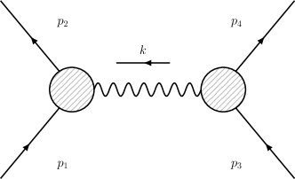
Figure 2: Tree-level singularity for one-graviton exchange

At 1PM or tree level, the leading-singularity prescription reduces to a $t$-channel residue equivalent to one-graviton exchange Cachazo:2017jef . The reason that this leads to classical effects is that the $O(t^{0})$ piece, which is dropped, is ultralocal after a Fourier transform Donoghue:1994dn ; Neill:2013wsa . In contrast to the one-loop case, the HCL defined as the leading order in $t$ is trivially implemented from the fact that the computation is done under the support of the factorization channel. Following sections 3.1 and 4.2 of Guevara:2017csg , the LS for the amplitude (75) with one graviton exchange is obtained by gluing two massive higher-spin three-point amplitudes at minimal coupling, see figure 2. These amplitudes are now given in the exponential form by eqs. (44) and (45) in the chiral basis. Summing over helicities, we have

$$\hat{\cal M}_{4}^{(s_{a},s_{b})} =\frac{1}{t}\bigg{[}\hat{\cal M}_{3}^{(s_{a})}(p_{1},-p_{2},k^{-})\otimes\hat{\cal M}_{3}^{(s_{b})}(p_{3},-p_{4},-k^{+})$$ (83)

$$\qquad~{}+\hat{\cal M}_{3}^{(s_{a})}(p_{1},-p_{2},k^{+})\otimes\hat{\cal M}_{3}^{(s_{b})}(p_{3},-p_{4},-k^{-})\bigg{]}$$

$$=\frac{m_{a}^{2}m_{b}^{2}}{t}\bigg{[}\frac{x_{a}^{2}}{x_{b}^{2}}\exp\!\bigg{(}i\frac{k_{\mu}\varepsilon^{-}_{\nu}J^{\mu\nu}_{a}}{p_{a}\cdot\varepsilon^{-}}\bigg{)}+\frac{x_{b}^{2}}{x_{a}^{2}}\exp\!\bigg{(}{-i}\frac{k_{\mu}\varepsilon^{-}_{\nu}J^{\mu\nu}_{b}}{p_{b}\cdot\varepsilon^{-}}\bigg{)}\bigg{]}.$$

Here we will take the limit where both massive particles’ spin quantum numbers ($s_{a}$ and $s_{b}$) go to infinity. After using eqs. (67) and (68) valid on the three-point kinematics, we can rewrite the exponents in a form independent of the polarization vector:

$$+i\frac{k_{\mu}\varepsilon^{-}_{\nu}J^{\mu\nu}_{a}}{p_{a}\cdot\varepsilon^{-}} =-2i\frac{k_{\mu}\varepsilon^{-}_{\nu}S^{\mu\nu}_{a}}{p_{a}\cdot\varepsilon^{-}}=+2a_{a}\cdot k=+2i\epsilon_{\mu\nu\rho\sigma}\frac{p_{a}^{\mu}p_{b}^{\nu}k^{\rho}a_{a}^{\sigma}}{m_{a}m_{b}\gamma v}=+2i\boldsymbol{k}\times\hat{\boldsymbol{p}}\cdot\boldsymbol{a}_{a},$$ (84a)

$${-i}\frac{k_{\mu}\varepsilon^{-}_{\nu}J^{\mu\nu}_{b}}{p_{b}\cdot\varepsilon^{-}} =+2i\frac{k_{\mu}\varepsilon^{-}_{\nu}S^{\mu\nu}_{b}}{p_{b}\cdot\varepsilon^{-}}=-2a_{b}\cdot k=-2i\epsilon_{\mu\nu\rho\sigma}\frac{p_{a}^{\mu}p_{b}^{\nu}k^{\rho}a_{b}^{\sigma}}{m_{a}m_{b}\gamma v}=-2i\boldsymbol{k}\times\hat{\boldsymbol{p}}\cdot\boldsymbol{a}_{b}.$$ (84b)

Here we used the on-shell equality $i\epsilon_{\mu\nu\rho\sigma}p_{a}^{\mu}p_{b}^{\nu}k^{\rho}a^{\sigma}=m_{a}m_{b}\sqrt{\gamma^{2}-1}\>\!(k\cdot a)$ to reintroduce the Levi-Civita tensor and thus to expose the scalar triple products in the center-of-mass frame, where $\hat{\boldsymbol{p}}$ is the unit vector in the direction of the relative momentum. Moreover, recall that on the three-point helicity factors satisfy the seemingly contradictory conditions $x_{a}/x_{b}=\gamma(1+v)$ and $x_{b}/x_{a}=\gamma(1-v)$, as indicated by eqs. (79) and (80). Finally, restoring the prefactor of $-(\kappa/2)^{2}=-8\pi G$, and dividing by the normalization factor arising from the generalized expectation value as in eq. (70),

$$(\varepsilon_{1}\cdot\varepsilon_{2})(\varepsilon_{3}\cdot\varepsilon_{4})~{}\rightarrow~{}\exp\!\Big{(}i\boldsymbol{k}\times\hat{\boldsymbol{p}}\cdot(\boldsymbol{a}_{a}-\boldsymbol{a}_{b})\Big{)}$$ (85)

(with the relative sign due to the direction of $k$), we obtain

$$\langle{\cal M}_{4}\rangle=8\pi G\frac{m_{a}^{2}m_{b}^{2}}{-t}\gamma^{2}\sum_{\pm}(1\pm v)^{2}\exp\!\Big{(}{\pm i}\boldsymbol{k}\times\hat{\boldsymbol{p}}\cdot(\boldsymbol{a}_{a}+\boldsymbol{a}_{b})\Big{)}.$$ (86)

Inserting this into the scattering-angle formula (82) gives

$$\theta_{\text{tree}} =-\frac{GE}{v^{2}}\sum_{\pm}(1\pm v)^{2}\frac{\partial~{}}{\partial b}\int\!\frac{d^{2}\boldsymbol{k}}{2\pi\boldsymbol{k}^{2}}\exp\!\Big{(}i\boldsymbol{k}\cdot\big{[}\boldsymbol{b}\pm\hat{\boldsymbol{p}}\times(\boldsymbol{a}_{a}+\boldsymbol{a}_{b})\big{]}\Big{)}$$ (87)

$$=\frac{GE}{v^{2}}\sum_{\pm}(1\pm v)^{2}\frac{\partial~{}}{\partial b}\bigg{[}\log\big{|}\boldsymbol{b}\pm\hat{\boldsymbol{p}}\times(\boldsymbol{a}_{a}+\boldsymbol{a}_{b})\big{|}=\log\big{(}b\pm(a_{a}+a_{b})\big{)}\bigg{]}$$

$$=\frac{GE}{v^{2}}\sum_{\pm}\frac{(1\pm v)^{2}}{b\pm(a_{a}+a_{b})},$$

having used $\hat{\boldsymbol{p}}\times\boldsymbol{a}=a\boldsymbol{b}/b$ for both spins in the aligned-spin configuration. This precisely matches the result for the 1PM aligned-spin binary-black-hole scattering angle found in Vines:2017hyw .

Finally, let us emphasize that, as stated in the introduction, this already differs from the strategy implemented in e.g. Holstein:2008sx ; Vaidya:2014kza , where the full tree-level amplitude for $s=\{\frac{1}{2},1,2\}$ was computed in the first place. Only then it was expanded in the NR limit $k=(0,\boldsymbol{k})\to 0$ under the COM frame. The evaluation of spin effects requires tracking subleading orders in the momentum transfer $\boldsymbol{k}$ (denoted there by $\!\vec{\,q}$), which in general contain both classical and quantum pieces, depending on whether they include the corresponding power of the spin vector. This is precisely what the LS singles out by dropping the (quantum) contraction $t=k^{2}$ in favor of the (classical) tensor structures $\sim k^{n}S^{n}$. At tree level this is equivalent to set the HCL $t=0$, but at one loop the HCL is needed to drop further quantum contributions from the LS, as we shall explain in the next subsection.

3.4 Second post-Minkowskian order

In this section we derive a compact form for the 2PM (or $\mathcal{O}(G^{2})$) aligned-spin scattering angle. It is obtained from the one-loop version of the four-point amplitude (75) through the triangle leading singularity proposed in Guevara:2017csg for computing its classical piece. The LS is now given by a contour integral for a single complex variable $y$ that remains in the loop integration after cutting the three propagators of figure 3:

$$\ell^{2}(y)=m_{b}^{2},\qquad(p_{3}-\ell(y))^{2}=0,\qquad(p_{4}-\ell(y))^{2}=0.$$ (88)

It was argued in Bjerrum-Bohr:2013bxa ; Cachazo:2017jef ; Guevara:2017csg that for the spinless case the Compton amplitude for identical helicities leads to no classical contribution. This fact is also true for arbitrary spin, as will be proven somewhere else. This implies that only the opposite-helicity case treated in section 2.3 is needed, together with three-point interactions. The derivation is thus valid (to describe minimally coupled elementary particles) at least up to $\mathcal{O}(a_{a}^{4})$ and to all orders in $a_{b}$, where $a_{a}$ is the rescaled spin of the particle that appears in the Compton amplitude, and $a_{b}$ is the spin of other particle. As explained already in Arkani-Hamed:2017jhn ; Guevara:2017csg and emphasized in section 2.3 the Compton amplitude needs the introduction of contact terms for $s_{a}>2$. Nevertheless, the exponential structure found already for $s_{a}\leq 2$ fits very nicely into the Fourier transform and leads to a compact formula for the scattering function, which can be computed directly once the multipole operators have been identified. The final formula resums all orders in both spins, but is not justified starting at $\mathcal{O}(a_{a}^{5})$. We finally expand in spins and find perfect agreement with the linear- and quadratic-order-in-spin results of Bini:2018ywr and Vines:2018gqi . The computation of the possible contributions to the LS from contact terms arising in the higher-spin Compton amplitude is left for future work.

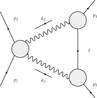
Figure 3: Triangle leading-singularity configuration

Our strategy is to identify the spin-multipole-coupling operators $\boldsymbol{k}\times\hat{\boldsymbol{p}}\cdot\boldsymbol{a}_{a}$ and $\boldsymbol{k}\times\hat{\boldsymbol{p}}\cdot\boldsymbol{a}_{b}$ in the exponential form of the three and four point amplitudes entering the triangle leading singularity, see figure 3. This is done on the support of the Holomorphic Classical Limit, which accounts for a null momentum transfer $k^{2}=0$ and recovers the three-point kinematics studied in section 2. The soft expansion in $k$ accounts for a simultaneous expansion in both powers of spin.

Let us first recap the triangle leading singularity, also introducing a more economic formulation of it. It consists of a contour integral obtained by gluing three-point amplitudes with the Compton amplitude. Our starting point is the expression

$$\frac{i(\kappa/2)^{4}}{8m_{b}\sqrt{-t}}\int_{\Gamma_{\rm{LS}}}\!\frac{dy}{2\pi y}\hat{\cal M}_{4}^{(s_{a})}(p_{1},-p_{2},k_{3}^{+},k_{4}^{-})\otimes\hat{\cal M}_{3}^{(s_{b})}(p_{3},-\ell,-k_{3}^{-})\frac{|\ell\rangle^{2s}\langle\ell|^{2s}\!}{m_{b}^{2s}}\hat{\cal M}_{3}^{(s_{b})}(-p_{4},\ell,-k_{4}^{+}),$$ (89)

where we have inserted the operator $|\ell\rangle\langle\ell|$ in-between the three-point amplitudes to denote operator multiplication, in the same sense as in section 2.1. Here $\Gamma_{\rm{LS}}$ is the leading-singularity contour that can be obtained at either $|y|=\epsilon$ or $|y|\rightarrow\infty$. The loop momenta, together with their corresponding spinors, are functions of $y$ given by eq. (3.17) of Guevara:2017csg . Here we will only need the following limits:

$$|k_{3}] =\frac{1}{2}|k](1+y)+{\cal O}\bigg{(}\frac{\sqrt{-t}}{m_{b}}\bigg{)},\qquad\quad\langle k_{3}|=\frac{1}{2y}\langle k|(1+y)+{\cal O}\bigg{(}\frac{\sqrt{-t}}{m_{b}}\bigg{)},$$

$$|k_{4}] =\frac{1}{2}|k](1-y)+{\cal O}\bigg{(}\frac{\sqrt{-t}}{m_{b}}\bigg{)},\qquad\quad\langle k_{4}|=-\frac{1}{2y}\langle k|(1-y)+{\cal O}\bigg{(}\frac{\sqrt{-t}}{m_{b}}\bigg{)},$$ (90)

$$\langle k_{3}k_{4}\rangle =\frac{\sqrt{-t}}{y}+{\cal O}\bigg{(}\frac{t}{m_{b}^{2}}\bigg{)},\qquad\!\qquad\langle k_{4}|p_{1}|k_{3}]=\frac{m_{a}\gamma}{2y}[2y-v(1+y^{2})]\sqrt{-t}+{\cal O}\bigg{(}\frac{t}{m_{b}^{2}}\bigg{)}.$$

Recall that at $t=0$ the momentum transfer reads $k=|k]\langle k|$ and the scaling of the spinors $|k]$, $\langle k|$ is fixed by the condition (79). In turn, this fixes the little-group scaling of both internal gravitons $k_{3}$ and $k_{4}$. We can now insert the exponential expressions (for $s_{a}\leq 2$) and evaluate the scalar pieces, obtaining

$$\frac{i(\kappa/2)^{4}}{8m_{b}\sqrt{-t}}\!\int_{\Gamma_{\rm{LS}}}\!\frac{dy}{2\pi y}{\cal M}_{4}^{(0)}(p_{1},-p_{2},k_{3}^{+},k_{4}^{-}){\cal M}_{3}^{(0)}(p_{3},-{\ell},-k_{3}^{-}){\cal M}_{3}^{(0)}(-p_{4},{\ell},-k_{4}^{+})$$ (91)

$$\qquad\qquad\!\quad\times\exp\!\bigg{(}i\frac{k_{4\mu}\varepsilon_{4\nu}^{-}J_{a}^{\mu\nu}}{p_{1}\cdot\varepsilon_{4}^{-}}\bigg{)}\otimes\exp\!\bigg{(}{-i}\frac{k_{3\mu}\varepsilon_{3\nu}^{-}J_{b}^{\mu\nu}}{p_{3}\cdot\varepsilon_{3}^{-}}\bigg{)}$$

$$=-\frac{i\kappa^{4}m_{a}^{2}m_{b}^{3}\gamma^{2}}{2^{9}v^{2}\sqrt{-t}}\!\int_{\Gamma_{\rm{LS}}}\!\!\frac{dy\,[2y-v(1+y^{2})]^{4}}{2\pi y^{3}(1-y^{2})^{2}}\exp\!\bigg{(}i\frac{k_{4\mu}\varepsilon_{4\nu}^{-}J_{a}^{\mu\nu}}{p_{1}\cdot\varepsilon_{4}^{-}}\bigg{)}\otimes\exp\!\bigg{(}{-i}\frac{k_{3\mu}\varepsilon_{3\nu}^{-}J_{b}^{\mu\nu}}{p_{3}\cdot\varepsilon_{3}^{-}}\bigg{)},$$

to leading orders in $t$.

Before proceeding to compute the GEV, let us clarify an important point. Recall that in the tree-level case the exponential operator was truncated at order $2s$ in the expansion. The infinite spin limit did not alter the lower orders in the exponential but simply accounted for promoting such finite number of terms to a full series. We assume such condition still holds for the Compton amplitude, that is, the first five orders reproducing the exponential expansion are not spoiled in the infinite spin limit. The reason is that at arbitrary spin, the introduction of contact terms is only needed to cancel the spurious pole coming from the exponent, which appears as a pole in the amplitude only at fifth order.

With the previous consideration, the above operator formula in the infinite spin limit is fourth-order exact in the expansion of the left exponential and fully exact in the expansion of the right exponential. Let us now proceed to evaluate the exponents of both. The exponential factor on the right can be obtained straight at $t=0$ kinematics. In fact, using

$$k_{3}=\frac{(1+y)^{2}}{4y}k,$$ (92)

we find

$$\exp\!\bigg{(}{-i}\frac{k_{3\mu}\varepsilon_{3\nu}^{-}J_{b}^{\mu\nu}}{p_{3}\cdot\varepsilon_{3}^{-}}\bigg{)}=\exp\!\bigg{(}{-i}\frac{(1+y)^{2}}{4y}\frac{k_{\mu}\varepsilon_{\nu}^{-}J_{b}^{\mu\nu}}{p_{3}\cdot\varepsilon^{-}}\bigg{)}=\exp\!\bigg{(}{-i}\frac{(1+y)^{2}}{2y}\boldsymbol{k}\times\hat{\boldsymbol{p}}\cdot\boldsymbol{a}_{b}\bigg{)},$$ (93)

where the polarization vector $\varepsilon_{3}^{-}$ for $k_{3}$ can be taken as the vector $\varepsilon^{-}$ for $k$, up to a scale that cancels. We have again identified $k_{\mu}\varepsilon_{\nu}J_{b}^{\mu\nu}/(p_{3}\cdot\varepsilon_{3})=2\boldsymbol{k}\times\hat{\boldsymbol{p}}\cdot\boldsymbol{a}_{b}$ as the classical operator that will enter the GEV, whereas the $y$ dependence contributes to the contour integral.

Now, recall that the left exponential corresponds to the Compton amplitude and was fixed in section 2.3 using $k_{3}\cdot\varepsilon_{4}=0$, i.e.

$$\varepsilon_{4}^{-}=-\sqrt{2}\frac{|k_{3}]\langle k_{4}|}{[k_{3}k_{4}]},$$ (94)

which is singular at $t=0$. In order to evaluate, it we will need the following trick. First note that at $t\neq 0$ the numerator is gauge invariant, hence we can write

$$k_{4\mu}\varepsilon_{4\nu}^{-}J_{a}^{\mu\nu}=k_{4\mu}\hat{\varepsilon}_{4\nu}^{-}J_{a}^{\mu\nu},$$ (95)

where

$$\hat{\varepsilon}_{4}^{-}=-\sqrt{2}\frac{|r]\langle k_{4}|}{[r\;\!k_{4}]}$$ (96)

and $|r]$ is some reference spinor such that $[r\;\!k_{4}]\neq 0$. This means that in the limit we have

$$\lim_{t\rightarrow 0}\frac{k_{4\mu}\varepsilon_{4\nu}^{-}J_{a}^{\mu\nu}}{p_{1}\cdot\varepsilon_{4}^{-}} = \big{(}k_{4\mu}\hat{\varepsilon}_{4\nu}^{-}J_{a}^{\mu\nu}\big{)}_{t=0}\lim_{t\rightarrow 0}(p_{1}\cdot\varepsilon_{4}^{-})^{-1}$$ (97)

$$= \bigg{(}\frac{k_{4\mu}\hat{\varepsilon}_{4\nu}^{-}J_{a}^{\mu\nu}}{p_{1}\cdot\hat{\varepsilon}_{4}^{-}}\bigg{)}_{t=0}\times(p_{1}\cdot\hat{\varepsilon}_{4}^{-})\big{|}_{t=0}\lim_{t\rightarrow 0}(p_{1}\cdot\varepsilon_{4}^{-})^{-1}\,.$$

The limit can be evaluated directly using eq. (90). We find

$$\lim_{t\rightarrow 0}(p_{1}\cdot\varepsilon_{4}^{-})=-\frac{\gamma m_{a}}{2\sqrt{2}y^{2}}\big{[}2y-v(1+y^{2})\big{]}.$$ (98)

On the other hand, recall that at $t=0$ we recover three-particle kinematics for $p_{1}$, $p_{2}$ and $k$. This means that the combination

$$(p_{1}\cdot\hat{\varepsilon}_{4}^{-})\big{|}_{t=0}=-\frac{[r|p_{1}|k_{4}\rangle}{\sqrt{2}[r\;\!k_{4}]}\bigg{|}_{t=0}=+\frac{1}{y}\frac{[r|p_{1}|k\rangle}{\sqrt{2}[r\;\!k]}$$ (99)

is independent of the choice of $r$. Using eq. (80) we can identify this factor with

$${-}\frac{1}{y}(p_{1}\cdot\varepsilon^{-})=-\frac{\gamma m_{a}}{\sqrt{2}y}(1+v),$$ (100)

Putting all together in (97) and using $k_{4}=-\frac{(1-y)^{2}}{4y}k$, we have

$$\lim_{t\rightarrow 0}\frac{k_{4\mu}\varepsilon_{4\nu}^{-}J_{a}^{\mu\nu}}{p_{1}\cdot\varepsilon_{4}^{-}} =\bigg{(}\frac{k_{4\mu}\hat{\varepsilon}_{4\nu}^{-}J_{a}^{\mu\nu}}{p_{1}\cdot\hat{\varepsilon}_{4}^{-}}\bigg{)}_{t=0}\times\frac{1}{y}(p_{1}\cdot\varepsilon^{-})\times\frac{2\sqrt{2}y^{2}}{\gamma m_{a}}\big{[}2y-v(1+y^{2})\big{]}^{-1}$$ (101)

$$=-\frac{(1-y)^{2}(1+v)}{4y-2v(1+y^{2})}\bigg{(}\frac{k_{\mu}\varepsilon_{\nu}^{-}J_{a}^{\mu\nu}}{p_{1}\cdot\varepsilon^{-}}\bigg{)}=-\frac{(1-y)^{2}(1+v)}{2y-v(1+y^{2})}\boldsymbol{k}\times\hat{\boldsymbol{p}}\cdot\boldsymbol{a}_{a}.$$

Attaching the same normalization (85) as in the previous section in order to compute the GEV, we write the leading order (i.e. dropping $\mathcal{O}(t^{0}$) terms) of our contour integral as

$${-}\frac{i\kappa^{4}m_{a}^{2}m_{b}^{3}\gamma^{2}}{2^{9}v^{2}\sqrt{-t}}\!\int_{\Gamma_{\rm{LS}}}\!\!\frac{dy\,[2y-v(1+y^{2})]^{4}}{2\pi y^{3}(1-y^{2})^{2}}\exp\!\bigg{(}{-i}\frac{1+y^{2}-2vy}{2y-v(1+y^{2})}\boldsymbol{k}\times\hat{\boldsymbol{p}}\cdot\boldsymbol{a}_{a}-i\frac{1+y^{2}}{2y}\boldsymbol{k}\times\hat{\boldsymbol{p}}\cdot\boldsymbol{a}_{b}\bigg{)}.$$ (102)

As already explained, $\Gamma_{\rm{LS}}$ can be chosen as a contour around zero or infinity. This inversion accounts for a parity conjugation of the amplitude, and the equivalence follows from parity invariance of the triangle diagram Cachazo:2017jef . Here let us unify both descriptions by means of the change of variables

$$z=\frac{1+y^{2}}{2y}.$$ (103)

Both contours around $y=\infty$ and $y=0$ are mapped to $z=\infty$. At the same time the polynomial structure gets reduced to at most quadratic, at the cost of introducing a branch cut in the integral. We now have the one-loop triangle contribution as

$$\langle{\cal M}_{\triangleleft}\rangle=-4\pi^{2}\frac{G^{2}m_{a}^{2}m_{b}^{3}}{\sqrt{-t}}\int_{\Gamma_{\rm{LS}}}\frac{dz}{2\pi i}\frac{\gamma^{2}(1-vz)^{4}}{v^{2}(z^{2}-1)^{3/2}}\exp\!\bigg{(}{-i}\frac{z-v}{1-vz}\boldsymbol{k}\times\hat{\boldsymbol{p}}\cdot\boldsymbol{a}_{a}-iz\boldsymbol{k}\times\hat{\boldsymbol{p}}\cdot\boldsymbol{a}_{b}\bigg{)},$$ (104)

which now incorporates the second helicity assignment for the exchanged gravitons. We have also inserted a factor of $-4$ to account for the HCL difference between a triangle integral and its leading singularity. Note that the branch cut singularity is induced by the massive propagators inside the Compton amplitude and does not lead to classical contributions. The essential singularity at $z=1/v$ is induced by the unphysical pole $p_{1}\cdot\varepsilon_{4}$ in the exponential expansion. We take the contour around infinity to be $\Gamma_{\rm{LS}}=\{|z|=R\}$ for some large but finite radius, $R>1/v$, for reasons we will explain in a moment. Then the contribution to the scattering angle (82) reads

$$\theta_{\triangleleft} =\pi G^{2}E\frac{m_{b}}{2v^{4}}\frac{\partial}{\partial b}\int_{\Gamma_{\rm{LS}}}\!\frac{dz}{2\pi i}\frac{(1-vz)^{4}}{(z^{2}-1)^{3/2}}\int\!\!\frac{d^{2}\boldsymbol{k}}{2\pi|\boldsymbol{k}|}\exp\!\Big{(}i\boldsymbol{k}\cdot\!\Big{[}\boldsymbol{b}-z\hat{\boldsymbol{p}}\times\boldsymbol{a}_{b}-\frac{z-v}{1-vz}\,\hat{\boldsymbol{p}}\times\boldsymbol{a}_{a}\Big{]}\Big{)}$$

$$=\pi G^{2}E\frac{m_{b}}{2v^{4}}\frac{\partial}{\partial b}\int_{\Gamma_{\rm{LS}}}\!\frac{dz}{2\pi i}\frac{(1-vz)^{4}}{(z^{2}-1)^{3/2}}\Big{|}b-za_{b}-\frac{z-v}{1-vz}a_{a}\Big{|}^{-1},$$ (105)

where we have specialized to aligned spins. The total one-loop contribution to the scattering angle is $\theta_{\triangleleft}+\theta_{\triangleright}$, where $\theta_{\triangleright}$ is obtained by exchanging $m_{a}\leftrightarrow m_{b}$ and $a_{a}\leftrightarrow a_{b}$.

Let us now discuss the choice of contour $\Gamma_{\rm{LS}}$ in

$$\int_{\Gamma_{\rm{LS}}}\!\frac{dz}{2\pi i}\frac{(1-vz)^{4}}{(z^{2}-1)^{3/2}}\Big{|}b-za_{b}-\frac{z-v}{1-vz}a_{a}\Big{|}^{-1}\!=\frac{1}{va}\int_{\Gamma_{\rm{LS}}}\!\frac{dz}{2\pi i}\frac{(vz-1)^{5}}{(z^{2}-1)^{3/2}(z-z_{+})(z-z_{-})},$$ (106a)

where

$$z_{+}+z_{-}=\frac{bv+a_{a}+a_{b}}{va_{b}},\qquad\quad z_{+}z_{-}=\frac{b+va_{a}}{va_{b}}.$$ (106b)

The root $z_{+}$ is distinguished from $z_{-}$ by demanding $z_{+}\to\infty$ as $a_{b}\to 0$. We now show that the appropriate leading singularity in the contour integral is given by the residues at $z_{+}$ and $\infty$, by ensuring the consistency of the small-spin expansion. If we were to take an expansion around $a_{a},a_{b}\to 0$ the poles at $z_{+}$ and $z_{-}$ would disappear at every order, leaving poles only at $z=\infty$ and $z=1/v$ together with the branch cut at $z\in(-1,1)$. In that case, the leading-singularity prescription in the integral (104) simply grabs the pole at $z=\infty$ and drops the branch cut contribution together with the pole at $z=1/v$. The non-expanded expression (106a) resums part of the contributions from both $z=\infty$ and $z={1}/{v}$ into poles located at $z_{+}$ and $z_{-}$, respectively. This can be seen by noticing that $z_{+}\to\infty$ and $z_{-}\to 1/v$ as $a_{a},a_{b}\rightarrow 0$. This is the reason we consider a contour at finite radius $R>1/v$ in eq. (104), so that, as long as $R<z_{+}$ as well, the contour integral can be evaluated from the poles at $z=\infty$ and $z=z_{+}$.

With this contour prescription, evaluating the integral in eq. (105) yields the explicit results given by eq. (12) in the introductory summary. Let us stress that the formulas (105) and (12) can only be expected to be valid up to fourth order in $a_{a}$. Nevertheless, they condense non-trivial information for the scattering angle up to that order into a simple contour integral. We have checked that these results precisely match the one-loop linear-in-spin classical computation of Bini:2018ywr , as well as the conjectural one-loop quadratic-in-spin expression given in Vines:2018gqi , based on results from the exact quadrupolar test-black-hole limit Bini:2017pee expanded to order $G^{2}$ and on next-to-next-to-leading-order post-Newtonian results Levi:2016ofk ; Levi:2015ixa .

4 Discussion

In this work we have presented a new connection between extended soft theorems and conservative classical gravitational observables, in particular for scattering of spinning black holes. This extends the approach initiated in Cachazo:2017jef ; Guevara:2017csg to construct such quantities in an economic way through leading singularities. It also complements the general picture regarding the extraction of classical results from on-shell methods, provided e.g. in BjerrumBohr:2005jr ; Neill:2013wsa ; Cheung:2018wkq .

It is clear that a more precise definition is needed for the generalized expectation value that we used. Our construction can be thought as the average of an operator ${\cal O}$ as given by two particle states in the scattering amplitude, which is mapped to the expectation value of a classical observable ${\cal O}_{\text{cl}}=\langle\cal O\rangle$. Interestingly, this matches their effective counterpart, as computed for instance in the worldline formalism, in the case where the operator ${\cal O}_{\text{cl}}$ is constant Vines:2017hyw ; Damour:2017zjx . An extension of the GEV may be needed to incorporate time dependence, such as what occurs with classical momentum deflection or spin holonomy Bini:2018ywr .

The natural desired extension of the leading-singularity method is the computation of higher orders, both in loops and powers of spin. Examples of higher-loop leading singularities were computed for gravitational theories in Cachazo:2017jef , so it would be interesting to see if these can be also applied to compute classical observables. On the other hand, extending the range of validity in powers of spin is now clearly related to the problem of understanding deeper orders in the soft expansion. More precisely, it is known that these orders depend both on the matter content and the coupling to gravity Laddha:2017ygw ; Sen:2017xjn , hence one could hope that such problem is tractable at least for matter minimally coupled to gravity Arkani-Hamed:2017jhn , thus describing black holes. Our methodology clearly resembles a soft bootstrap approach Rodina:2018pcb , and it would be desirable to formally implement it via recursion relations Elvang:2018dco ; Carballo-Rubio:2018bmu .

It was already pointed out in Vaidya:2014kza that amplitudes for massive spin-$s$ particles lead to a classical potential for bodies with spin-induced multipoles such as black holes or neutron stars. The amplitudes match the classical potential up to the $2^{2s}$-pole level, or up to order $S^{2s}$, where $S$ is the body’s intrinsic angular momentum:

• a scalar particle corresponds to a monopole (with no higher multipoles);

• a spin-1/2 particle adds only a dipole $\propto S$, yielding the ${\cal O}(S^{1})$ spin-orbit effects which are universal (body-independent) in gravity;

• a spin-1 particle further adds a spin-induced quadrupole $\propto S^{2}$, specifically matching the quadrupole of a spinning black hole when constructed with minimal coupling. Note that the quadrupole level corresponds to the order at which the soft theorem stops being universal.

• a spin-3/2 particle adds a black-hole octupole $\propto S^{3}$, etc.

The complete spin-multipole series of a black hole is seemingly obtained by taking the limit $s~{}\to~{}\infty$ for a massive spin-$s$ particle minimally coupled to gravity. This correlation was shown by Vaidya Vaidya:2014kza with explicit calculations at leading post-Newtonian orders, corresponding to the nonrelativistic limits of tree-level amplitudes, up to the spin-2 or $S^{4}$ level. In this paper, we have provided further evidence that this correspondence holds, fully relativistically, to all orders in spin at tree level, and for at least the first few orders in spin at one-loop order. It is, however, not yet clear why we should expect this correspondence between classical black holes and minimally coupled quantum particles with $s\to\infty$ and $\hbar\to 0$, and to what extent we should expect it to hold.

It was found in He:2014bga , by means of a BCFW argument, that in the MHV sector of gravity amplitudes there is also a natural exponential completion of the soft theorem. A general statement for gravity amplitudes is however still missing. There are a few evident problems for the naive extrapolation of the formula (1) to higher orders. As we have seen, increasing the powers of angular momentum, encoded in the gauge-invariant combination $(k_{\mu}\varepsilon_{\nu}J_{i}^{\mu\nu})$, requires decreasing the powers of the numerator $(p\cdot\varepsilon_{i})$, which generates unphysical poles. Moreover, the first two orders enjoy gauge invariance thanks to fundamental conservation laws corresponding to the linear and angular momenta of the scattering particles Cachazo:2014fwa . Reinserting powers of $(p\cdot\varepsilon_{i})$ in higher orders would then impose additional constraints that go beyond these conservation laws. Therefore, when exponentiating the soft factor, a very specific choice of the polarization vectors is required. This is precisely what is done in He:2014bga , where this choice arises naturally from a BCFW deformation. A second problem that we dealt with here is the sum over different particles, which destroys the realization of the exponential as an overall factor acting on ${\cal M}_{n-1}$. We showed that in the cases of interest for computing the scattering angle at tree level and one loop, these two problems can be overcome by a judicious choice of the polarization vectors.

An obvious question which arises from this construction is whether it is possible to establish a link between BMS symmetries studied at null/spatial infinity Strominger:2013jfa ; He:2014laa ; Kapec:2014opa ; Dumitrescu:2015fej ; Campiglia:2016hvg ; Strominger:2017zoo (or at the black hole horizon Hawking:2016msc ; Penna:2018gfx ) and classical observables arising from massive amplitudes. The natural candidate for such a connection is radiative effects Porto:2016pyg ; Goldberger:2016iau ; Goldberger:2017frp ; Luna:2017dtq ; Shen:2018ebu , as explored in Laddha:2018rle from the point of view of soft theorems. Finally, it would be also interesting to see a link between the exponentiation presented here and the exponentiation of IR divergences Weinberg:1965nx ; Frenkel:1976bj ; Bern:1995ix ; Ciafaloni:2015xsr ; Strominger:2017zoo that has been known in QED for a long time. The latter one has recently appeared in the computation of tail effects from the EFT perspective Goldberger:2009qd ; Porto:2016pyg ; Levi:2018nxp .

Appendix A Three-point amplitude with spin-1 matter

Here we compute the three-point amplitude (13) starting from the massive spin-1 Lagrangian

$${\cal L}=-\frac{1}{4}F_{\mu\nu}F^{\mu\nu}+\frac{m^{2}}{2}A_{\mu}A^{\mu},$$ (107)

where $F^{\mu\nu}=\partial^{\mu}A^{\nu}-\partial^{\nu}A^{\mu}$. In order to compute the minimal cubic vertex to gravity, one needs to the extract the energy-momentum tensor sourced by this field. In principle, this can be done by covariantizing this action, i.e. by promoting $\partial_{\mu}\rightarrow\nabla_{\mu}$, and then inspecting the metric variation, $T_{\mu\nu}=\frac{2}{\sqrt{-g}}\frac{\partial(\sqrt{-g}\mathcal{L})}{\partial g^{\mu\nu}}$. Let us, however, take an alternative route of computing the energy-momentum tensor directly in flat space. The reason is that this procedure will explicitly identify the contribution of the intrinsic angular momentum of the particle.

A textbook application of Noether’s theorem for translations yields the following tensor

$$T_{N}^{\mu\nu}=-F^{\mu\sigma}\partial^{\nu}A_{\sigma}-\eta^{\mu\nu}{\cal L}\qquad\Rightarrow\qquad\partial_{\mu}T_{N}^{\mu\nu}=0.$$ (108)

Its contraction with an on-shell graviton, $\varepsilon_{\mu\nu}T_{N}^{\mu\nu}$, fails to give the correct three-point amplitude, as opposed to the one obtained from covariantization. The reason is that $T_{N}^{\mu\nu}$ lacks symmetry in its indices (notice e.g. $\partial_{\nu}T_{N}^{\mu\nu}\neq 0$), therefore its orbital angular momentum $L^{\lambda\,\mu\nu}=x^{\mu}T_{N}^{\lambda\nu}-x^{\nu}T_{N}^{\lambda\mu}$ is not conserved. Let us fix that by generalizing $T_{N}^{\mu\nu}$ to a larger class of tensors that are all conserved due to eq. (108):

$$T^{\mu\nu}=T_{N}^{\mu\nu}+\partial_{\lambda}B^{\lambda\mu\,\nu},\qquad\quad B^{\lambda\mu\,\nu}=-B^{\mu\lambda\,\nu}\qquad\Rightarrow\qquad\partial_{\mu}T^{\mu\nu}=0,$$ (109)

where the Belinfante tensor $B^{\mu\nu\rho}$ 1940Phy…..7..449B ; Rosenfeld:1940 may be adjusted to yield a symmetric energy-momentum tensor matching the gravitational one. To do that, we apply Noether’s theorem to Lorentz transformations. The conservation of the total angular momentum $L^{\lambda\,\mu\nu}+S^{\lambda\,\mu\nu}$ then implies

$$T_{N}^{\mu\nu}-T_{N}^{\nu\mu}=-\partial_{\lambda}S^{\lambda\,\mu\nu},\qquad\quad S^{\lambda\,\mu\nu}=-i\frac{\partial{\cal L}}{\partial(\partial_{\lambda}A^{\sigma})}\Sigma^{\mu\nu,\sigma}_{~{}~{}~{}~{}~{}\tau}A^{\tau}=iF^{\lambda\sigma}\Sigma^{\mu\nu}_{\sigma\tau}A^{\tau}.$$ (110)

Here $\Sigma_{\mu\nu}$ are the Lorentz generators $\Sigma^{\mu\nu,\sigma}_{~{}~{}~{}~{}~{}\tau}=i[\eta^{\mu\sigma}\delta^{\nu}_{\tau}-\eta^{\nu\sigma}\delta^{\mu}_{\tau}]$ that will help us identify the spin contribution inside the three-point amplitude. Imposing that the corrected tensor $T^{\mu\nu}$ be symmetric now yields the condition $\partial_{\lambda}B^{\lambda[\mu\,\nu]}=\frac{1}{2}\partial_{\lambda}S^{\lambda\,\mu\nu}$, which is solved by

$$B^{\lambda\mu\,\nu}=\frac{1}{2}\big{[}S^{\lambda\,\mu\nu}+S^{\mu\,\nu\lambda}-S^{\nu\,\lambda\mu}\big{]}.$$ (111)

Contracting the resulting energy-momentum tensor with a traceless symmetric graviton $h_{\mu\nu}$ and integrating by parts, we obtain the gravitational interaction vertex

$$-h_{\mu\nu}T^{\mu\nu}=h_{\mu\nu}F^{\mu\sigma}\partial^{\nu}A_{\sigma}-i(\partial_{\lambda}h_{\mu\nu})F^{\nu\sigma}\Sigma^{\lambda\mu}_{\sigma\tau}A^{\tau},$$ (112)

where we suppress the coupling-constant factor $\kappa/2$. Its momentum-space version in the scattering amplitude gives the following contributions:

$$h_{\mu\nu}F^{\mu\sigma}\partial^{\nu}A_{\sigma} \,\rightarrow\,-(p_{2}\!\cdot\varepsilon_{3})\big{[}(p_{1}\!\cdot\varepsilon_{3})(\varepsilon_{1}\!\cdot\varepsilon_{2})-(p_{1}\!\cdot\varepsilon_{2})(\varepsilon_{1}\!\cdot\varepsilon_{3})\big{]}+(1\leftrightarrow 2),$$ (113a)

$$\!\!\!-i(\partial_{\mu}h_{\nu\rho})F^{\rho\sigma}\Sigma^{\mu\nu}_{\sigma\tau}A^{\tau} \,\rightarrow\,ip_{3\mu}\varepsilon_{3\nu}\big{[}(p_{1}\!\cdot\varepsilon_{3})(\varepsilon_{1}\!\cdot\!\Sigma^{\mu\nu}\!\cdot\!\varepsilon_{2})-(\varepsilon_{1}\!\cdot\varepsilon_{3})(p_{1}\!\cdot\!\Sigma^{\mu\nu}\!\cdot\!\varepsilon_{2})\big{]}+(1\leftrightarrow 2).\!\!$$ (113b)

where the transverse polarization vectors $\varepsilon_{1}$ and $\varepsilon_{2}$ correspond to the massive spin-1 matter and two copies of $\varepsilon_{3}$ belong to the massless graviton. Putting the above terms together and using the three-point on-shell kinematic conditions $p_{1}\cdot p_{3}=p_{2}\cdot p_{3}=0$, we obtain the amplitude

$${\cal M}_{3}=2(p_{1}\!\cdot\varepsilon)\big{[}(p_{1}\!\cdot\varepsilon)(\varepsilon_{1}\!\cdot\varepsilon_{2})-2p_{3\mu}\varepsilon_{3\nu}\varepsilon_{1}^{[\mu}\varepsilon_{2}^{\nu]}\big{]},$$ (114)

The second term in eq. (114) comes from $\varepsilon_{1}\!\cdot\!\Sigma^{\mu\nu}\!\cdot\!\varepsilon_{2}^{\tau}=2i\varepsilon_{1}^{[\mu}\varepsilon_{2}^{\nu]}$, which in appendix B we interpret as a spin expectation value, so it can be regarded as the spin contribution to the gravitational interaction.

Appendix B Spin tensor for spin-1 matter

Here we construct the spin tensor for a massive spin-1 particle for the three-particle kinematics of section 2.1. The starting point is the one-particle expectation value of the angular-momentum operator in the quantum-mechanical sense:

$$S_{p}^{\mu\nu}=\frac{\langle p|\Sigma^{\mu\nu}|p\rangle}{\langle p|p\rangle}=\frac{\varepsilon_{p\>\!\sigma}^{*}\Sigma^{\mu\nu,\sigma}_{~{}~{}~{}~{}\;\tau}\varepsilon_{p}^{\tau}}{\varepsilon_{p}^{*}\!\cdot\varepsilon_{p}}=2i\varepsilon_{p}^{*[\mu}\varepsilon_{p}^{\nu]},\qquad\quad\Sigma^{\mu\nu,\sigma}_{~{}~{}~{}~{}~{}\tau}=i[\eta^{\mu\sigma}\delta^{\nu}_{\tau}-\eta^{\nu\sigma}\delta^{\mu}_{\tau}],$$ (115)

where for now we suppress the spin-projection/little-group labels of the states. We also used the Lorentz generators $\Sigma^{\mu\nu}$ in the vector representation. Due to the transversality of the both massive polarization vectors, $p\cdot\varepsilon_{p}=0$, this spin tensor immediately satisfies the SSC (16).

Now a natural way to extend eq. (115) to the case of two different states (one incoming with momentum $p_{1}$ and one outgoing with $p_{2}$) is to introduce a generalized expectation value such that it gives one for a unit operator:

$$S_{12}^{\mu\nu}=\frac{\langle 2|\Sigma^{\mu\nu}|1\rangle}{\langle 2|1\rangle}=\frac{\varepsilon_{2\>\!\sigma}^{*}\Sigma^{\mu\nu,\sigma}_{~{}~{}~{}~{}\;\tau}\varepsilon_{1}^{\tau}}{\varepsilon_{2}^{*}\cdot\varepsilon_{1}}=\frac{2i\varepsilon_{2}^{*[\mu}\varepsilon_{1}^{\nu]}}{\varepsilon_{2}^{*}\cdot\varepsilon_{1}}.$$ (116)

Since in section 2 we consider all momenta incoming, we suppress the conjugation sign and rewrite the above as

$$S_{12}^{\mu\nu}=-2i\varepsilon_{1}^{[\mu}\varepsilon_{2}^{\nu]}/(\varepsilon_{1}\!\cdot\varepsilon_{2}),$$ (118)

which is the (normalized) angular momentum contribution obtained in appendix A from Noether’s theorem. Now in a classical computation Vines:2017hyw it is desirable to consider a spin tensor that satisfies the spin supplementary condition (16). Although eq. (118) is a legitimate definition, it does not satisy the covariant SSC (16) with respect to the average momentum $p=(p_{1}-p_{2})/2$ of the massive particle before and after graviton emission:

$$p_{\mu}S_{12}^{\mu\nu}=-\frac{i}{2}\big{(}(k\cdot\varepsilon_{2})\varepsilon_{1}^{\nu}+(k\cdot\varepsilon_{1})\varepsilon_{2}^{\nu}\big{)}/(\varepsilon_{1}\!\cdot\varepsilon_{2})\neq 0,$$ (119)

where $k=-p_{1}-p_{2}$ is the momentum transfer. However, the spin tensor is intrinsically ambiguous, as the separation between the orbital and intrinsic pieces of the total angular momentum is relativistically frame-dependent. In a classical setting, for instance, the reference point for the intrinsic angular momentum of a spatially extended body (as opposed to its overall orbital momentum about the origin) is at its center of mass, but it gets shifted by a frame change (see e.g. Steinhoff:2015ksa ). This ambiguity allows the spin tensor to be transformed as $S^{\mu\nu}\rightarrow S^{\mu\nu}+p^{[\mu}r^{\nu]}$, where the difference $p^{[\mu}r^{\nu]}$ for some vector $r^{\nu}$ accounts for the relative shift between $S^{\mu\nu}$ and $L^{\mu\nu}\sim p^{[\mu}\partial/\partial p_{\nu]}$. Adjusting $r^{\nu}$ to accommodate for the SSC (16), we obtain

$$S^{\mu\nu}=S_{12}^{\mu\nu}+\frac{2}{m^{2}}p_{\lambda}S_{12}^{\lambda[\mu}p^{\nu]}=-\frac{i}{\varepsilon_{1}\!\cdot\varepsilon_{2}}\bigg{\{}2\varepsilon_{1}^{[\mu}\varepsilon_{2}^{\nu]}-\frac{1}{m^{2}}p^{[\mu}\big{(}(k\cdot\varepsilon_{2})\varepsilon_{1}+(k\cdot\varepsilon_{1})\varepsilon_{2}\big{)}^{\nu]}\bigg{\}},$$ (120)

where we have used that $p^{2}=m^{2}$ for a null momentum transfer $k$. Finally, we note that in the classical limit $k\rightarrow 0$ we retrieve the spin tensor (118) as the covariant-SSC one.

Appendix C Angular-momentum operator

Here we consider the total angular momentum

$$\!J_{\mu\nu}=L_{\mu\nu}+S_{\mu\nu},\qquad\quad L_{\mu\nu}^{\text{pos.}}=2ix_{[\mu}\frac{\partial~{}}{\partial x^{\nu]}}$$ (121)

in terms of the spinor-helicity variables. The starting point is the momentum-space form of the orbital piece

$$L_{\mu\nu}=2ip_{[\mu}\frac{\partial~{}}{\partial p^{\nu]}}=p_{\sigma}\Sigma_{\mu\nu,~{}\tau}^{~{}~{}~{}\sigma}\frac{\partial~{}}{\partial p_{\tau}},$$ (122)

in which we encounter the Lorentz generators $\Sigma^{\mu\nu}$ again. Since $\Sigma_{\mu\nu,\sigma\tau}$ is antisymmetric in both pairs of indices, we notice the subtle difference in signs between the actions of the differential and algebraic operators, $L_{\mu\nu}p^{\rho}=-\Sigma_{\mu\nu,~{}\sigma}^{~{}~{}~{}\rho}p^{\sigma}$, also valid for $J_{\mu\nu}$ below.

Massless Case

Let us warm up with the case of a massless $k^{\mu}=\langle k|\sigma^{\mu}|k]/2$. The spinorial version of the angular momentum (122) is Witten:2003nn

$$J^{\mu\nu}=\bigg{[}\lambda^{\alpha}\sigma_{~{}~{}~{}\alpha}^{\mu\nu,~{}\,\beta}\frac{\partial~{}}{\partial\lambda^{\beta}}+\tilde{\lambda}_{\dot{\alpha}}\bar{\sigma}^{\mu\nu,\dot{\alpha}}_{~{}~{}~{}~{}\,\dot{\beta}}\frac{\partial~{}}{\partial\tilde{\lambda}_{\dot{\beta}}}\bigg{]},$$ (123)

where the matrices

$$\sigma_{~{}~{}~{}\alpha}^{\mu\nu,~{}\,\beta}=\frac{i}{4}\big{(}\sigma^{\mu}_{\alpha\dot{\gamma}}\bar{\sigma}^{\nu,\dot{\gamma}\beta}-\sigma^{\nu}_{\alpha\dot{\gamma}}\bar{\sigma}^{\mu,\dot{\gamma}\beta}\big{)},\qquad\quad\bar{\sigma}^{\mu\nu,\dot{\alpha}}_{~{}~{}~{}~{}\,\dot{\beta}}=\frac{i}{4}\big{(}\bar{\sigma}^{\mu,\dot{\alpha}\gamma}\sigma^{\nu}_{\gamma\dot{\beta}}-\bar{\sigma}^{\nu,\dot{\alpha}\gamma}\sigma^{\mu}_{\gamma\dot{\beta}}\big{)}$$ (124)

are the left-handed and right-handed representations of the Lorentz-group algebra. Note that the spinor map $\{\lambda_{\alpha},\tilde{\lambda}_{\dot{\alpha}}\}\rightarrow k^{\mu}$ is not invertible for massless particles, but we can still use the chain rule

$$\frac{\partial~{}}{\partial\lambda^{\alpha}}=\frac{\partial k^{\mu}}{\partial\lambda^{\alpha}}\frac{\partial~{}}{\partial k^{\mu}}=\frac{1}{2}\sigma^{\mu}_{\alpha\dot{\beta}}\tilde{\lambda}^{\dot{\beta}}\frac{\partial~{}}{\partial k^{\mu}},\qquad\quad\frac{\partial~{}}{\partial\tilde{\lambda}_{\dot{\alpha}}}=\frac{1}{2}\bar{\sigma}^{\mu,\dot{\alpha}\beta}\lambda_{\beta}\frac{\partial~{}}{\partial k^{\mu}}$$ (125)

to check the consistency between eqs. (122) and (123). Namely, the action of spinorial generator on a function of momentum $k^{\mu}$ coincides with that of the vectorial one.

The generator (123), which can be more concisely written in spinor indices as

$$J_{\alpha\dot{\alpha},\beta\dot{\beta}}=\sigma^{\mu}_{\alpha\dot{\alpha}}\sigma^{\nu}_{\beta\dot{\beta}}J_{\mu\nu}=2i\bigg{[}\lambda_{(\alpha}\frac{\partial~{}}{\partial\lambda^{\beta)}}\epsilon_{\dot{\alpha}\dot{\beta}}+\epsilon_{\alpha\beta}\tilde{\lambda}_{(\dot{\alpha}}\frac{\partial~{}}{\partial\tilde{\lambda}^{\dot{\beta})}}\bigg{]},$$ (126)

has more information than its momentum-space counterpart, as it cares about the helicity of the massless particle. For instance, when we write the polarization tensors in terms of spinor-helicity variables,

$$\varepsilon^{+}_{\alpha\dot{\alpha}}=\sqrt{2}\;\!\frac{|r\rangle_{\alpha}[k|_{\dot{\alpha}}}{\langle r\;\!k\rangle},\qquad\quad\varepsilon^{-}_{\alpha\dot{\alpha}}=-\sqrt{2}\;\!\frac{|k\rangle_{\alpha}[r|_{\dot{\alpha}}}{[r\;\!k]},$$ (127)

we do not regard them as functions of $k^{\mu}$ but rather of its spinors $\lambda_{\alpha}$ and $\tilde{\lambda}_{\dot{\alpha}}$. Of course, an integer spin should not by itself depend on the auxiliary spinors. Fortunately, we can show that the action of the differential operator (126) is precisely that of the algebraic generator $\Sigma_{\mu\nu}$, which constitutes the intrinsic angular momentum

$$(\varepsilon S^{\mu\nu})_{\tau}=\varepsilon_{\sigma}\Sigma^{\mu\nu,\sigma}_{~{}~{}~{}~{}~{}\tau}=2i\varepsilon^{[\mu}\delta^{\nu]}_{\tau}\qquad\Rightarrow\qquad(\varepsilon S_{\alpha\dot{\alpha},\beta\dot{\beta}})_{\gamma\dot{\gamma}}=2i[\varepsilon_{\alpha\dot{\alpha}}\epsilon_{\beta\gamma}\epsilon_{\dot{\beta}\dot{\gamma}}-\epsilon_{\alpha\gamma}\epsilon_{\dot{\alpha}\dot{\gamma}}\varepsilon_{\beta\dot{\beta}}].$$ (128)

Specializing to the negative-helicity case for concreteness, we indeed find

$$J_{\alpha\dot{\alpha},\beta\dot{\beta}}\varepsilon^{-}_{\gamma\dot{\gamma}}=(\varepsilon^{-}S_{\alpha\dot{\alpha},\beta\dot{\beta}})_{\gamma\dot{\gamma}}+\frac{2\sqrt{2}i}{[q\;\!k]^{2}}\epsilon_{\alpha\beta}[q|_{\dot{\alpha}}[q|_{\dot{\beta}}|k\rangle_{\gamma}[k|_{\dot{\gamma}}.$$ (129)

Here the last term is a gauge contribution explicitly proportional to $k_{\gamma\dot{\gamma}}$, so it can be discarded in a physical amplitude.

Therefore, we conclude that the spinorial differential operator (126) incorporates both the orbital and intrinsic contributions, so it is the total angular-momentum operator.

Massive Case

It is direct to generalize the above discussion to massive momenta $p^{\mu}=\langle p^{a}|\sigma^{\mu}|p_{a}]/2$ Conde:2016izb . The angular-momentum operator in the space of massive spinors $\{\lambda_{\alpha}^{a},\tilde{\lambda}_{\dot{\beta}}^{b}\}$ is given by

$$J^{\mu\nu}=\bigg{[}\lambda^{\alpha a}\sigma_{~{}~{}~{}\alpha}^{\mu\nu,~{}\,\beta}\frac{\partial~{}}{\partial\lambda^{\beta a}}+\tilde{\lambda}_{\dot{\alpha}}^{\,a}\bar{\sigma}^{\mu\nu,\dot{\alpha}}_{~{}~{}~{}~{}\,\dot{\beta}}\frac{\partial~{}}{\partial\tilde{\lambda}_{\dot{\beta}}^{a}}\bigg{]},\qquad\quad J_{\alpha\dot{\alpha},\beta\dot{\beta}}=2i\bigg{[}\lambda_{(\alpha}^{~{}a}\frac{\partial~{}}{\partial\lambda^{\beta)a}}\epsilon_{\dot{\alpha}\dot{\beta}}+\epsilon_{\alpha\beta}\tilde{\lambda}_{(\dot{\alpha}}^{~{}a}\frac{\partial~{}}{\partial\tilde{\lambda}^{\dot{\beta})a}}\bigg{]}.$$ (130)

This operator is by construction invariant under the little group ${\rm SU}(2)$. Using the chain rule

$$\frac{\partial~{}}{\partial\lambda^{\alpha a}}=\frac{\partial p^{\mu}}{\partial\lambda^{\alpha a}}\frac{\partial~{}}{\partial p^{\mu}}=\frac{1}{2}\sigma^{\mu}_{\alpha\dot{\beta}}\tilde{\lambda}^{\dot{\beta}}_{a}\frac{\partial~{}}{\partial p^{\mu}},\qquad\quad\frac{\partial~{}}{\partial\tilde{\lambda}_{\dot{\alpha}}^{a}}=-\frac{1}{2}\bar{\sigma}^{\mu,\dot{\alpha}\beta}\lambda_{\beta a}\frac{\partial~{}}{\partial p^{\mu}},$$ (131)

it is again easy to check that the action on a function of $p_{\alpha\dot{\beta}}=\lambda_{\alpha}^{a}\epsilon_{ab}\tilde{\lambda}_{\dot{\beta}}^{b}$ is the same as that of eq. (122). Finally, the action on polarization tensors can be tested to be a Lorentz transformation. The spin-$s$ tensors are parametrized in terms of massive spinor-helicity variables as

$$\varepsilon_{\alpha_{1}\dot{\alpha}_{1}\ldots\alpha_{s}\dot{\alpha}_{s}}^{a_{1}\ldots a_{2s}}=\frac{2^{s/2}}{m^{s}}\lambda_{\alpha_{1}}^{(a_{1}}\tilde{\lambda}_{\dot{\alpha}_{1}}^{a_{2}}\cdots\lambda_{\alpha_{s}}^{a_{2s-1}}\tilde{\lambda}_{\dot{\alpha}_{s}}^{a_{2s})}.$$ (132)

with an obvious extension by an additional factor of Dirac spinor Arkani-Hamed:2017jhn ; Ochirov:2018uyq for half-integer spins. Indeed, since $J^{\mu\nu}$ is a first-order differential operator, it distributes when acting on $\varepsilon^{a_{1}\cdots a_{2s}}$ and naturally expands into the left- and right-handed Lorentz generators:

$$J^{\mu\nu}\varepsilon_{\alpha_{1}\dot{\alpha}_{1}\ldots\alpha_{s}\dot{\alpha}_{s}}^{a_{1}\ldots a_{2s}}=\frac{2^{s/2}}{m^{s}}\bigg{\{}\Big{[}\epsilon_{\alpha_{1}\beta}\big{(}\lambda^{\alpha(a_{1}}\sigma_{~{}~{}~{}\alpha}^{\mu\nu,~{}\,\beta}\big{)}\Big{]}\tilde{\lambda}_{\dot{\alpha}_{1}}^{a_{2}} \cdots\lambda_{\alpha_{s}}^{a_{2s-1}}\tilde{\lambda}_{\dot{\alpha}_{s}}^{a_{2s})}$$ (133)

$$+\lambda_{\alpha_{1}}^{(a_{1}}\Big{[}\tilde{\lambda}_{\dot{\alpha}}^{a_{2}}\bar{\sigma}^{\mu\nu,\dot{\alpha}}_{~{}~{}~{}~{}\,\dot{\alpha_{2}}}\Big{]} \cdots\lambda_{\alpha_{s}}^{a_{2s-1}}\tilde{\lambda}_{\dot{\alpha}_{s}}^{a_{2s})}+\ldots\bigg{\}}.$$

References

- (1) F. Cachazo and A. Strominger, Evidence for a New Soft Graviton Theorem, 1404.4091.
- (2) S. Weinberg, Infrared photons and gravitons, Phys. Rev. 140 (1965) B516.
- (3) F. E. Low, Scattering of light of very low frequency by systems of spin 1/2, Phys. Rev. 96 (1954) 1428.
- (4) F. E. Low, Bremsstrahlung of very low-energy quanta in elementary particle collisions, Phys. Rev. 110 (1958) 974.
- (5) D. J. Gross and R. Jackiw, Low-Energy Theorem for Graviton Scattering, Phys. Rev. 166 (1968) 1287.
- (6) R. Jackiw, Low-Energy Theorems for Massless Bosons: Photons and Gravitons, Phys. Rev. 168 (1968) 1623.
- (7) C. D. White, Factorization Properties of Soft Graviton Amplitudes, JHEP 05 (2011) 060 [1103.2981].
- (8) Z. Bern, S. Davies, P. Di Vecchia and J. Nohle, Low-Energy Behavior of Gluons and Gravitons from Gauge Invariance, Phys. Rev. D90 (2014) 084035 [1406.6987].
- (9) A. Laddha and A. Sen, Sub-subleading Soft Graviton Theorem in Generic Theories of Quantum Gravity, JHEP 10 (2017) 065 [1706.00759].
- (10) A. Sen, Soft Theorems in Superstring Theory, JHEP 06 (2017) 113 [1702.03934].
- (11) M. Bianchi, S. He, Y.-t. Huang and C. Wen, More on Soft Theorems: Trees, Loops and Strings, Phys. Rev. D92 (2015) 065022 [1406.5155].
- (12) Y. Hamada and G. Shiu, Infinite Set of Soft Theorems in Gauge-Gravity Theories as Ward-Takahashi Identities, Phys. Rev. Lett. 120 (2018) 201601 [1801.05528].
- (13) Z.-Z. Li, H.-H. Lin and S.-Q. Zhang, Infinite Soft Theorems from Gauge Symmetry, Phys. Rev. D98 (2018) 045004 [1802.03148].
- (14) A. Strominger, On BMS Invariance of Gravitational Scattering, JHEP 07 (2014) 152 [1312.2229].
- (15) T. He, V. Lysov, P. Mitra and A. Strominger, BMS supertranslations and Weinberg’s soft graviton theorem, JHEP 05 (2015) 151 [1401.7026].
- (16) F. Cachazo and E. Y. Yuan, Are Soft Theorems Renormalized?, 1405.3413.
- (17) D. Kapec, V. Lysov, S. Pasterski and A. Strominger, Semiclassical Virasoro symmetry of the quantum gravity -matrix, JHEP 08 (2014) 058 [1406.3312].
- (18) T. T. Dumitrescu, T. He, P. Mitra and A. Strominger, Infinite-Dimensional Fermionic Symmetry in Supersymmetric Gauge Theories, 1511.07429.
- (19) M. Campiglia and A. Laddha, Subleading soft photons and large gauge transformations, JHEP 11 (2016) 012 [1605.09677].
- (20) A. Strominger, Lectures on the Infrared Structure of Gravity and Gauge Theory, 1703.05448.
- (21) M. Campiglia and A. Laddha, Asymptotic charges in massless QED revisited: A view from Spatial Infinity, JHEP 05 (2019) 207 [1810.04619].
- (22) A. Laddha and A. Sen, Gravity Waves from Soft Theorem in General Dimensions, JHEP 09 (2018) 105 [1801.07719].
- (23) M. J. Duff, Quantum Tree Graphs and the Schwarzschild Solution, Phys. Rev. D7 (1973) 2317.
- (24) N. E. J. Bjerrum-Bohr, J. F. Donoghue and B. R. Holstein, Quantum corrections to the Schwarzschild and Kerr metrics, Phys. Rev. D68 (2003) 084005 [hep-th/0211071].
- (25) D. Neill and I. Z. Rothstein, Classical Space-Times from the S Matrix, Nucl.Phys. B877 (2013) 177 [1304.7263].
- (26) N. E. J. Bjerrum-Bohr, P. H. Damgaard, G. Festuccia, L. Planté and P. Vanhove, General Relativity from Scattering Amplitudes, Phys. Rev. Lett. 121 (2018) 171601 [1806.04920].
- (27) V. Vaidya, Gravitational spin Hamiltonians from the S matrix, Phys. Rev. D91 (2015) 024017 [1410.5348].
- (28) B. R. Holstein and A. Ross, Spin Effects in Long Range Gravitational Scattering, 0802.0716.
- (29) A. Guevara, Holomorphic Classical Limit for Spin Effects in Gravitational and Electromagnetic Scattering, JHEP 04 (2019) 033 [1706.02314].
- (30) B. R. Holstein and A. Ross, Spin Effects in Long Range Electromagnetic Scattering, 0802.0715.
- (31) F. Cachazo and A. Guevara, Leading Singularities and Classical Gravitational Scattering, 1705.10262.
- (32) J. Vines, Scattering of two spinning black holes in post-Minkowskian gravity, to all orders in spin, and effective-one-body mappings, Class. Quant. Grav. 35 (2018) 084002 [1709.06016].
- (33) T. Damour, Gravitational scattering, post-Minkowskian approximation and Effective One-Body theory, Phys. Rev. D94 (2016) 104015 [1609.00354].
- (34) D. A. Kosower, B. Maybee and D. O’Connell, Amplitudes, Observables, and Classical Scattering, JHEP 02 (2019) 137 [1811.10950].
- (35) N. Arkani-Hamed, T.-C. Huang and Y.-t. Huang, Scattering amplitudes for all masses and spins, 1709.04891.
- (36) D. Bini and T. Damour, Gravitational spin-orbit coupling in binary systems, post-Minkowskian approximation and effective one-body theory, Phys. Rev. D96 (2017) 104038 [1709.00590].
- (37) T. Damour, High-energy gravitational scattering and the general relativistic two-body problem, Phys. Rev. D97 (2018) 044038 [1710.10599].
- (38) D. Bini and T. Damour, Gravitational spin-orbit coupling in binary systems at the second post-Minkowskian approximation, Phys. Rev. D98 (2018) 044036 [1805.10809].
- (39) C. Cheung, I. Z. Rothstein and M. P. Solon, From Scattering Amplitudes to Classical Potentials in the Post-Minkowskian Expansion, Phys. Rev. Lett. 121 (2018) 251101 [1808.02489].
- (40) J. Vines, J. Steinhoff and A. Buonanno, Spinning-black-hole scattering and the test-black-hole limit at second post-Minkowskian order, Phys. Rev. D99 (2019) 064054 [1812.00956].
- (41) K. Westpfahl, High-Speed Scattering of Charged and Uncharged Particles in General Relativity, Fortschritte der Physik 33 (1985) 417.
- (42) D. N. Kabat and M. Ortiz, Eikonal quantum gravity and Planckian scattering, Nucl. Phys. B388 (1992) 570 [hep-th/9203082].
- (43) R. Akhoury, R. Saotome and G. Sterman, High Energy Scattering in Perturbative Quantum Gravity at Next to Leading Power, 1308.5204.
- (44) W. M. Tulczyjew, Motion of multipole particles in general relativity theory, Acta Phys. Polon. 18 (1959) 393.
- (45) A. D. Fokker, Relativiteitstheorie. P. Noordhoff, Groningen, 1929.
- (46) N. Arkani-Hamed, F. Cachazo and J. Kaplan, What is the Simplest Quantum Field Theory?, JHEP 09 (2010) 016 [0808.1446].
- (47) B. R. Holstein, Factorization in graviton scattering and the ’natural’ value of the g-factor, gr-qc/0607058.
- (48) W. D. Goldberger, J. Li and S. G. Prabhu, Spinning particles, axion radiation, and the classical double copy, Phys. Rev. D97 (2018) 105018 [1712.09250].
- (49) S. Weinberg, Dynamic and Algebraic Symmetries, in Proceedings, 13th Brandeis University Summer Institute in Theoretical Physics, Lectures On Elementary Particles and Quantum Field Theory: Waltham, MA, USA, June 15 - July 24 1970, (Cambridge, Mass.), pp. 283–393, Deser, Stanley (ed.). Massachusetts Inst. of Tech. Press, 1970, https://mitpress.mit.edu/index.php?q=books/lectures-elementary-particles-and-quantum-field-theory.
- (50) A. Ochirov, Helicity amplitudes for QCD with massive quarks, JHEP 04 (2018) 089 [1802.06730].
- (51) E. Witten, Perturbative gauge theory as a string theory in twistor space, Commun.Math.Phys. 252 (2004) 189 [hep-th/0312171].
- (52) N. E. J. Bjerrum-Bohr, B. R. Holstein, J. F. Donoghue, L. Planté and P. Vanhove, Illuminating Light Bending, PoS CORFU2016 (2017) 077 [1704.01624].
- (53) J. F. Donoghue, General relativity as an effective field theory: The leading quantum corrections, Phys.Rev. D50 (1994) 3874 [gr-qc/9405057].
- (54) N. E. J. Bjerrum-Bohr, J. F. Donoghue and P. Vanhove, On-shell Techniques and Universal Results in Quantum Gravity, JHEP 02 (2014) 111 [1309.0804].
- (55) D. Bini, A. Geralico and J. Vines, Hyperbolic scattering of spinning particles by a Kerr black hole, Phys. Rev. D96 (2017) 084044 [1707.09814].
- (56) M. Levi and J. Steinhoff, Complete conservative dynamics for inspiralling compact binaries with spins at fourth post-Newtonian order, 1607.04252.
- (57) M. Levi and J. Steinhoff, Next-to-next-to-leading order gravitational spin-squared potential via the effective field theory for spinning objects in the post-Newtonian scheme, JCAP 1601 (2016) 008 [1506.05794].
- (58) N. Bjerrum-Bohr, D. C. Dunbar, H. Ita, W. B. Perkins and K. Risager, MHV-vertices for gravity amplitudes, JHEP 0601 (2006) 009 [hep-th/0509016].
- (59) L. Rodina, Scattering Amplitudes from Soft Theorems and Infrared Behavior, Phys. Rev. Lett. 122 (2019) 071601 [1807.09738].
- (60) H. Elvang, M. Hadjiantonis, C. R. T. Jones and S. Paranjape, Soft Bootstrap and Supersymmetry, JHEP 01 (2019) 195 [1806.06079].
- (61) R. Carballo-Rubio, F. Di Filippo and N. Moynihan, Taming higher-derivative interactions and bootstrapping gravity with soft theorems, 1811.08192.
- (62) S. He, Y.-t. Huang and C. Wen, Loop Corrections to Soft Theorems in Gauge Theories and Gravity, JHEP 12 (2014) 115 [1405.1410].
- (63) S. W. Hawking, M. J. Perry and A. Strominger, Soft Hair on Black Holes, Phys. Rev. Lett. 116 (2016) 231301 [1601.00921].
- (64) R. F. Penna, Near-horizon Carroll symmetry and black hole Love numbers, 1812.05643.
- (65) R. A. Porto, The effective field theorist’s approach to gravitational dynamics, Phys. Rept. 633 (2016) 1 [1601.04914].
- (66) W. D. Goldberger and A. K. Ridgway, Radiation and the classical double copy for color charges, Phys. Rev. D95 (2017) 125010 [1611.03493].
- (67) W. D. Goldberger, S. G. Prabhu and J. O. Thompson, Classical gluon and graviton radiation from the bi-adjoint scalar double copy, Phys. Rev. D96 (2017) 065009 [1705.09263].
- (68) A. Luna, I. Nicholson, D. O’Connell and C. D. White, Inelastic Black Hole Scattering from Charged Scalar Amplitudes, JHEP 03 (2018) 044 [1711.03901].
- (69) C.-H. Shen, Gravitational Radiation from Color-Kinematics Duality, JHEP 11 (2018) 162 [1806.07388].
- (70) J. Frenkel and J. C. Taylor, Exponentiation of Leading Infrared Divergences in Massless Yang-Mills Theories, Nucl. Phys. B116 (1976) 185.
- (71) Z. Bern and G. Chalmers, Factorization in one loop gauge theory, Nucl.Phys. B447 (1995) 465 [hep-ph/9503236].
- (72) M. Ciafaloni, D. Colferai, F. Coradeschi and G. Veneziano, Unified limiting form of graviton radiation at extreme energies, Phys. Rev. D93 (2016) 044052 [1512.00281].
- (73) W. D. Goldberger and A. Ross, Gravitational radiative corrections from effective field theory, Phys. Rev. D81 (2010) 124015 [0912.4254].
- (74) M. Levi, Effective Field Theories of Post-Newtonian Gravity: A comprehensive review, 1807.01699.
- (75) F. J. Belinfante, On the current and the density of the electric charge, the energy, the linear momentum and the angular momentum of arbitrary fields, Physica 7 (1940) 449.
- (76) L. Rosenfeld, Sur le tenseur D’Impulsion-Energie, Acad. Roy. Belg. Memoirs de Classes de Science 18 (1940) (fasc. 6).
- (77) J. Steinhoff, Spin gauge symmetry in the action principle for classical relativistic particles, 1501.04951.
- (78) E. Conde, E. Joung and K. Mkrtchyan, Spinor-Helicity Three-Point Amplitudes from Local Cubic Interactions, JHEP 08 (2016) 040 [1605.07402].