Bayesian Mean-parameterized Nonnegative Binary Matrix Factorization

Alberto Lumbreras Criteo AI Lab, France Louis Filstroff IRIT, Université de Toulouse, CNRS, France Cédric Févotte IRIT, Université de Toulouse, CNRS, France
Abstract

Binary data matrices can represent many types of data such as social networks, votes, or gene expression. In some cases, the analysis of binary matrices can be tackled with nonnegative matrix factorization (NMF), where the observed data matrix is approximated by the product of two smaller nonnegative matrices. In this context, probabilistic NMF assumes a generative model where the data is usually Bernoulli-distributed. Often, a link function is used to map the factorization to the [0,1]01[0,1] range, ensuring a valid Bernoulli mean parameter. However, link functions have the potential disadvantage to lead to uninterpretable models. Mean-parameterized NMF, on the contrary, overcomes this problem. We propose a unified framework for Bayesian mean-parameterized nonnegative binary matrix factorization models (NBMF). We analyze three models which correspond to three possible constraints that respect the mean-parameterization without the need for link functions. Furthermore, we derive a novel collapsed Gibbs sampler and a collapsed variational algorithm to infer the posterior distribution of the factors. Next, we extend the proposed models to a nonparametric setting where the number of used latent dimensions is automatically driven by the observed data. We analyze the performance of our NBMF methods in multiple datasets for different tasks such as dictionary learning and prediction of missing data. Experiments show that our methods provide similar or superior results than the state of the art, while automatically detecting the number of relevant components.

1 Introduction

Nonnegative matrix factorization (NMF) is a family of methods that approximate a nonnegative matrix 𝐕𝐕\mathbf{V} of size F×N𝐹𝑁{F\times N} as the product of two nonnegative matrices,

𝐕𝐖𝐇,𝐕𝐖𝐇\displaystyle\boldsymbol{\mathbf{V}}\approx\boldsymbol{\mathbf{WH}}, (1)

where 𝐖𝐖\mathbf{W} has size F×K𝐹𝐾F\times K, and 𝐇𝐇\mathbf{H} has size K×N𝐾𝑁{K\times N}, often referred to as the dictionary and the activation matrix, respectively. K𝐾K is usually chosen such that FK+KNFNmuch-less-than𝐹𝐾𝐾𝑁𝐹𝑁FK+KN\ll~{}FN, hence reducing the data dimension.

Such an approximation is often sought after by minimizing a measure of fit between the observed data 𝐕𝐕\mathbf{V} and its factorized approximation 𝐖𝐇𝐖𝐇\mathbf{WH}, i.e.,

𝐖,𝐇=argmin𝐖,𝐇D(𝐕|𝐖𝐇)s.t𝐖0,𝐇0,formulae-sequence𝐖𝐇subscriptargmin𝐖𝐇𝐷conditional𝐕𝐖𝐇s.t𝐖0𝐇0\displaystyle\boldsymbol{\mathbf{W}},\boldsymbol{\mathbf{H}}=\operatorname*{arg\,min}_{\boldsymbol{\mathbf{W,H}}}D(\boldsymbol{\mathbf{V}}|\boldsymbol{\mathbf{WH}})\quad\text{s.t}\quad\boldsymbol{\mathbf{W}}\geq 0,\quad\boldsymbol{\mathbf{H}}\geq 0, (2)

where D𝐷D denotes the cost function, and where the notation 𝐀0𝐀0\boldsymbol{\mathbf{A}}\geq 0 denotes nonnegativity of the entries of 𝐀𝐀\boldsymbol{\mathbf{A}}. Typical cost functions include the squared Euclidean distance and the generalized Kullback-Leiber divergence (Lee and Seung, 2001), the α𝛼\alpha-divergence (Cichocki et al., 2008) or the β𝛽\beta-divergence (Févotte and Idier, 2011). Most of these cost functions underlie a probabilistic model for the data, such that minimization of the cost function is equivalent to joint maximum likelihood estimation of the factors (Singh and Gordon, 2008), i.e.,

argmin𝐖,𝐇D(𝐕|𝐖𝐇)=argmax𝐖,𝐇p(𝐕|𝐖,𝐇),subscriptargmin𝐖𝐇𝐷conditional𝐕𝐖𝐇subscriptargmax𝐖𝐇𝑝conditional𝐕𝐖𝐇\displaystyle\operatorname*{arg\,min}_{\boldsymbol{\mathbf{W}},\boldsymbol{\mathbf{H}}}D(\boldsymbol{\mathbf{V}}|\boldsymbol{\mathbf{WH}})=\operatorname*{arg\,max}_{\boldsymbol{\mathbf{W,H}}}p(\boldsymbol{\mathbf{V}}|\boldsymbol{\mathbf{W}},\boldsymbol{\mathbf{H}}), (3)

where p𝑝p is a probability distribution. As such, so-called Bayesian NMF can be considered, where the factors 𝐖𝐖\mathbf{W} and 𝐇𝐇\mathbf{H} are assumed to be random variables with prior distributions, and inference is based on their posterior distribution, i.e.,

p(𝐖,𝐇|𝐕)=p(𝐕|𝐖,𝐇)p(𝐖,𝐇)/p(𝐕).𝑝𝐖conditional𝐇𝐕𝑝conditional𝐕𝐖𝐇𝑝𝐖𝐇𝑝𝐕\displaystyle p(\boldsymbol{\mathbf{W}},\boldsymbol{\mathbf{H}}|\boldsymbol{\mathbf{V}})=p(\boldsymbol{\mathbf{V}}|\boldsymbol{\mathbf{W}},\boldsymbol{\mathbf{H}})p(\boldsymbol{\mathbf{W}},\boldsymbol{\mathbf{H}})/p(\boldsymbol{\mathbf{V}}). (4)

This has notably been addressed for different models such as Poisson (Cemgil, 2009), additive Gaussian (Schmidt et al., 2009; Alquier and Guedj, 2017), or multiplicative Exponential (Hoffman et al., 2010).

In this paper, we are interested in Bayesian NMF for binary data matrices. Binary matrices may represent a large variety of data such as social networks, voting data, gene expression data, or binary images. As we shall see in Section 2, a common practice is to consider the model

p(𝐕|𝐖,𝐇)=f,nBernoulli(vfn|ϕ([𝐖𝐇]fn)),𝑝conditional𝐕𝐖𝐇subscriptproduct𝑓𝑛Bernoulliconditionalsubscript𝑣𝑓𝑛italic-ϕsubscriptdelimited-[]𝐖𝐇𝑓𝑛p(\mathbf{V}|\mathbf{W},\mathbf{H})=\prod_{f,n}\text{Bernoulli}\left(v_{fn}|\phi([\mathbf{WH}]_{fn})\right), (5)

where ϕitalic-ϕ\phi is a link function that maps the factorization 𝐖𝐇𝐖𝐇\mathbf{WH} to the [0,1]01[0,1] range.111Distributions used throughout the article are formally defined in Appendix A. Although link functions are convenient since they allow the factors to be unconstrained, and sometimes result in tractable problems, they sacrifice the mean-parameterization of the Bernoulli likelihood (i.e. 𝔼[𝐕|𝐖𝐇]=ϕ(𝐖𝐇)𝔼delimited-[]conditional𝐕𝐖𝐇italic-ϕ𝐖𝐇\mathbb{E}[\mathbf{V}|\mathbf{WH}]=\phi(\mathbf{WH}) instead of 𝔼[𝐕|𝐖𝐇]=𝐖𝐇𝔼delimited-[]conditional𝐕𝐖𝐇𝐖𝐇\mathbb{E}[\mathbf{V}|\mathbf{WH}]=\mathbf{WH}).

Mean-parameterized nonnegative binary matrix factorization (NBMF), however, does not rely on a link function —or equivalently, considers ϕ(𝐖𝐇)=𝐖𝐇italic-ϕ𝐖𝐇𝐖𝐇\phi(\boldsymbol{\mathbf{WH}})=\boldsymbol{\mathbf{WH}}— and assumes the likelihood of the data to be

p(𝐕|𝐖,𝐇)=f,nBernoulli(vfn|[𝐖𝐇]fn),𝑝conditional𝐕𝐖𝐇subscriptproduct𝑓𝑛Bernoulliconditionalsubscript𝑣𝑓𝑛subscriptdelimited-[]𝐖𝐇𝑓𝑛p(\mathbf{V}|\mathbf{W},\mathbf{H})=\prod_{f,n}\text{Bernoulli}(v_{fn}|[\mathbf{WH}]_{fn}),

which implies 𝔼[𝐕|𝐖𝐇]=𝐖𝐇𝔼delimited-[]conditional𝐕𝐖𝐇𝐖𝐇\mathbb{E}[\mathbf{V}|\mathbf{WH}]=\mathbf{WH}. Mean-parameterization is an interesting property of a model because it makes the decomposition easy to interpret. Besides, in a Bernoulli likelihood, the product 𝐖𝐇𝐖𝐇\mathbf{WH} —and, in this paper, the individual factors as well— can be interpreted as probabilities. An additional advantage of dealing with probabilities is that they lay in a linear, continuous space, where we can apply off-the-shelf clustering methods over the latent factors. For instance, in recommender systems, we may want to cluster users by latent musical preferences, or by the latent type of product they buy. Or we may want a user to see only those categories with a probability higher than some threshold.

Our contributions in this paper are the following:

  1. (a)

    we present a unified framework for three Bayesian mean-parameterized NBMF models that place three possible constraints on the factors;

  2. (b)

    we derive a collapsed Gibbs sampler as well as collapsed variational inference algorithms, which have never been considered for these models;

  3. (c)

    we discuss the extension of the models to a nonparametric setting —where the number of latent components does not need to be fixed a priori— and propose an approximation that shows excellent results with real data.

We test the performance of the models for different tasks in multiple datasets and show that our models give similar or superior results to the state of the art, while automatically detecting the number of relevant components. The datasets, the algorithms, and scripts to replicate all the reported results are available through an R package. 222https://github.com/alumbreras/NBMF

2 Related work

2.1 Logistic PCA family

One of the earliest probabilistic approaches to model binary data matrices comes from PCA-related methods. The reformulation of PCA as a probabilistic generative model with a Gaussian likelihood (Sammel et al., 1997; Tipping and Bishop, 1999) opened the door to considering other likelihoods such as Bernoulli models, which are more appropriate for binary observations. We refer to it as logistic PCA. The maximum likelihood estimator in the model is given by

vfnBernoulli(σ([𝐖𝐇]fn)),similar-tosubscript𝑣𝑓𝑛Bernoulli𝜎subscriptdelimited-[]𝐖𝐇𝑓𝑛\displaystyle v_{fn}\sim\text{Bernoulli}\left(\sigma\left([{\mathbf{W}}{\mathbf{H}}]_{fn}\right)\right), (6)

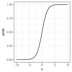
where σ𝜎\sigma is the logistic function σ(x)=1/(1+ex)𝜎𝑥11superscript𝑒𝑥\sigma(x)=1/(1+e^{-x}). Note that in this model the expectation is a non-linear transformation of the factors, such that 𝔼[𝐕|𝐖𝐇]=σ(𝐖𝐇)𝔼delimited-[]conditional𝐕𝐖𝐇𝜎𝐖𝐇\mathbb{E}[\boldsymbol{\mathbf{V}}|\boldsymbol{\mathbf{WH}}]=\sigma(\boldsymbol{\mathbf{WH}}).

There are multiple maximum likelihood estimation algorithms for logistic PCA. For instance, while Sammel et al. (1997) use a Monte-Carlo Expectation Minimization (MC-EM) algorithm, Tipping (1999) derives a faster variational EM (vEM) algorithm. Collins et al. (2002) generalize probabilistic PCA to the exponential family and propose a general algorithm that exploits the duality between likelihoods in the exponential family and Bregman divergences. Later, Schein et al. (2003) improved the algorithm of Collins et al. (2002), thanks to the optimization of a tight upper bound by Alternate Least Squares (ALS). Finally, note that inference could also be tackled with Polya-Gamma data augmentation schemes Polson et al. (2013).

Other models similar to logistic PCA have been proposed with various priors or constraints over the factors. Some examples are Hernandez-Lobato et al. (2014), where the factors are given Gaussian priors, Tomé et al. (2013), which allows one factor to have negative values, and Larsen and Clemmensen (2015), where both factors are nonnegative. Meeds et al. (2007) consider the same logistic link function but a three factor decomposition σ(𝐖𝐗𝐇\sigma(\mathbf{WXH}), where 𝐖𝐖\mathbf{W} and 𝐇𝐇\mathbf{H} are binary factors that represent cluster assignments, and 𝐗𝐗\mathbf{X} is a real-valued matrix that encodes the relations between the clusters. The expectation in these models is always 𝔼[𝐕|𝐖𝐇]=σ(𝐖𝐇)𝔼delimited-[]conditional𝐕𝐖𝐇𝜎𝐖𝐇\mathbb{E}[\boldsymbol{\mathbf{V}}|\boldsymbol{\mathbf{WH}}]=\sigma(\boldsymbol{\mathbf{WH}}) or 𝔼[𝐕|𝐖𝐗𝐇]=σ(𝐖𝐗𝐇)𝔼delimited-[]conditional𝐕𝐖𝐗𝐇𝜎𝐖𝐗𝐇\mathbb{E}[\boldsymbol{\mathbf{V}}|\boldsymbol{\mathbf{WXH}}]=\sigma(\boldsymbol{\mathbf{WXH}}).

2.2 Poisson matrix factorization

For practical reasons, some works have considered Poisson matrix factorization (PMF) techniques for binary data. In this case the binary nature of the data is ignored and a Poisson likelihood is considered:

vfnPoisson([𝐖𝐇]fn).similar-tosubscript𝑣𝑓𝑛Poissonsubscriptdelimited-[]𝐖𝐇𝑓𝑛\displaystyle v_{fn}\sim\text{Poisson}([{\mathbf{W}}{\mathbf{H}}]_{fn}). (7)

Different flavors of PMF have been proposed, in frequentists or Bayesian settings, and can be found, for example, in Lee and Seung (2001); Canny (2004); Cemgil (2009); Zhou et al. (2012); Gopalan et al. (2014, 2015). An advantage of PMF is that it is mean-parameterized, i.e., 𝔼[𝐕|𝐖𝐇]=𝐖𝐇𝔼delimited-[]conditional𝐕𝐖𝐇𝐖𝐇\mathbb{E}[\boldsymbol{\mathbf{V}}|\boldsymbol{\mathbf{WH}}]=\boldsymbol{\mathbf{WH}}. Another useful advantage is that inference algorithms need only iterate over non-zero values, which makes them very efficient for sparse matrices. In our case, a significant disadvantage is that it assigns non-zero probabilities to impossible observations (vfn>1)v_{fn}>1).

As we discussed above, a more reasonable choice consists in replacing the Poisson distribution with a Bernoulli distribution, possibly using some link function that maps the parameter into a [0,1]01[0,1] range, ensuring a valid Bernoulli parameter. Unfortunately, unlike Poisson models, zeroes and ones under Bernoulli likelihoods do not represent counts but classes —a zero can be considered as a no, while a one can be considered as a yes— and the algorithms need to iterate over all the elements of the observation matrix. To bypass this, Zhou (2015); Zhou et al. (2016) proposed using the alternative link function f(x)=1ex𝑓𝑥1superscript𝑒𝑥f(x)=1-e^{-x}, coined Bernoulli-Poisson, such that

vfnBernoulli(f([𝐖𝐇]fn)).similar-tosubscript𝑣𝑓𝑛Bernoulli𝑓subscriptdelimited-[]𝐖𝐇𝑓𝑛\displaystyle v_{fn}\sim\text{Bernoulli}\left(f\left([{\mathbf{W}}{\mathbf{H}}]_{fn}\right)\right). (8)

Thanks to the new link function, the model can be “augmented” to a Poisson model by introducing latent variables cfnsubscript𝑐𝑓𝑛c_{fn} such that

cfnsubscript𝑐𝑓𝑛\displaystyle c_{fn} Poisson([𝐖𝐇]fn)similar-toabsentPoissonsubscriptdelimited-[]𝐖𝐇𝑓𝑛\displaystyle\sim\text{Poisson}([{\mathbf{W}}{\mathbf{H}}]_{fn}) (9)
vfnsubscript𝑣𝑓𝑛\displaystyle v_{fn} =𝟙[cfn1],absent1delimited-[]subscript𝑐𝑓𝑛1\displaystyle=\mathbbm{1}[c_{fn}\geq 1], (10)

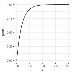
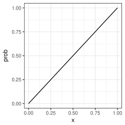
where 𝟙1\mathbbm{1} is the set indicator function. By placing conjugate Gamma priors over the factors, posteriors can be obtained by Gibbs sampling. Expectation in this model is 𝔼[𝐕|𝐖𝐇]=f(𝐖𝐇)𝔼delimited-[]conditional𝐕𝐖𝐇𝑓𝐖𝐇\mathbb{E}[\boldsymbol{\mathbf{V}}|\boldsymbol{\mathbf{WH}}]=f(\boldsymbol{\mathbf{WH}}). Figure 1 shows the logistic and Bernoulli-Poisson functions. Note that each link function has a different input domain, leading to different priors or constraints over the factors.
Refer to caption
(a) Identity
Refer to caption
(b) Logistic
Refer to caption
(c) Bernoulli-Poisson
Figure 1: Three possible link functions (identity induces mean-parameterization).

2.3 Bernoulli mean-parameterized matrix factorization

None of the above methods offers mean-parameterization and assumes a Bernoulli distribution over the data. The family of mean-parameterized Bernoulli models is the basis of the models presented in this paper. These models have first been introduced in Kabán and Bingham (2008) (binary ICA) and Bingham et al. (2009) (Aspect Bernoulli model) where the constraints kwfk=1,hkn[0,1]formulae-sequencesubscript𝑘subscript𝑤𝑓𝑘1subscript𝑘𝑛01\sum_{k}w_{fk}=1,h_{kn}\in[0,1], or vice versa, are imposed on the factors. The trick is that these constraints induce convex combinations of binary elements such that kwfkhkn[0,1]subscript𝑘subscript𝑤𝑓𝑘subscript𝑘𝑛01\sum_{k}w_{fk}h_{kn}\in[0,1], which gives a valid Bernoulli parameter. In Bingham et al. (2009) the constraints are imposed explicitly, and the maximum likelihood estimator is computed by using EM with an augmented version of the model. In Kabán and Bingham (2008) the constraint is imposed through Dirichlet and Beta priors over the factors, and Variational Bayes (VB) estimation of their posteriors is derived exploiting a similar augmentation scheme.

Table 1 presents a summary of the methods presented in Sections 2.1-2.3 that use a Bernoulli likelihood.

Table 1: Bernoulli matrix factorization methods considered in the literature. Bernoulli, Gamma, Dirichlet distributions are denoted as Ber, Ga, and Dir, respectively. Gradient refers to Gradient-based optimization.
Reference Likelihood Prior / Constr. Estimation
Sammel et al. (1997) Ber(σ([𝐖𝐇]fn))Ber𝜎subscriptdelimited-[]𝐖𝐇𝑓𝑛\text{Ber}(\sigma([\boldsymbol{\mathbf{WH}}]_{fn})) wfkNormal()similar-tosubscript𝑤𝑓𝑘Normalw_{fk}\sim\text{Normal}(\cdot) MC-EM
hknsubscript𝑘𝑛h_{kn}\in\mathbb{R}
Tipping (1999) Ber(σ([𝐖𝐇]fn))Ber𝜎subscriptdelimited-[]𝐖𝐇𝑓𝑛\text{Ber}(\sigma([\boldsymbol{\mathbf{W}}\boldsymbol{\mathbf{H}}]_{fn})) wfkNormal()similar-tosubscript𝑤𝑓𝑘Normalw_{fk}\sim\text{Normal}(\cdot) vEM
hknsubscript𝑘𝑛h_{kn}\in\mathbb{R}
Collins et al. (2002) Ber(σ([𝐖𝐇]fn))Ber𝜎subscriptdelimited-[]𝐖𝐇𝑓𝑛\text{Ber}(\sigma([\boldsymbol{\mathbf{W}}\boldsymbol{\mathbf{H}}]_{fn})) wfksubscript𝑤𝑓𝑘w_{fk}\in\mathbb{R} Gradient
hknsubscript𝑘𝑛h_{kn}\in\mathbb{R}
Schein et al. (2003) Ber(σ([𝐖𝐇]fn))Ber𝜎subscriptdelimited-[]𝐖𝐇𝑓𝑛\text{Ber}(\sigma([\boldsymbol{\mathbf{W}}\boldsymbol{\mathbf{H}}]_{fn})) wfksubscript𝑤𝑓𝑘w_{fk}\in\mathbb{R} ALS
hknsubscript𝑘𝑛h_{kn}\in\mathbb{R}
Meeds et al. (2007) Ber(σ([𝐖𝐗𝐇]fn))Ber𝜎subscriptdelimited-[]𝐖𝐗𝐇𝑓𝑛\text{Ber}(\sigma([\boldsymbol{\mathbf{W}}\boldsymbol{\mathbf{X}}\boldsymbol{\mathbf{H}}]_{fn})) wfkBer()similar-tosubscript𝑤𝑓𝑘Berw_{fk}\sim\text{Ber}(\cdot) Gibbs
hknBer()similar-tosubscript𝑘𝑛Berh_{kn}\sim\text{Ber}(\cdot)
Kabán and Bingham (2008) Ber([𝐖𝐇]fn)Bersubscriptdelimited-[]𝐖𝐇𝑓𝑛\text{Ber}([\boldsymbol{\mathbf{W}}\boldsymbol{\mathbf{H}}]_{fn}) wknBeta()similar-tosubscript𝑤𝑘𝑛Betaw_{kn}\sim\text{Beta}(\cdot) VB
𝐡nDir()similar-tosubscript𝐡𝑛Dir\boldsymbol{\mathbf{h}}_{n}\sim\text{Dir}(\cdot)
Bingham et al. (2009) Ber([𝐖𝐇]fn)Bersubscriptdelimited-[]𝐖𝐇𝑓𝑛\text{Ber}([\boldsymbol{\mathbf{W}}\boldsymbol{\mathbf{H}}]_{fn}) kwfk=1subscript𝑘subscript𝑤𝑓𝑘1\sum_{k}w_{fk}=1 EM
hkn[0,1]subscript𝑘𝑛01h_{kn}\in[0,1]
Tomé et al. (2013) Ber(σ([𝐖𝐇]fn))Ber𝜎subscriptdelimited-[]𝐖𝐇𝑓𝑛\text{Ber}(\sigma([\boldsymbol{\mathbf{W}}\boldsymbol{\mathbf{H}}]_{fn})) wfk+subscript𝑤𝑓𝑘subscriptw_{fk}\in\mathbb{R}_{+} Gradient
hknsubscript𝑘𝑛h_{kn}\in\mathbb{R}
Larsen and Clemmensen (2015) Ber(σ([𝐖𝐇]fn))Ber𝜎subscriptdelimited-[]𝐖𝐇𝑓𝑛\text{Ber}(\sigma([\boldsymbol{\mathbf{W}}\boldsymbol{\mathbf{H}}]_{fn})) wfk+subscript𝑤𝑓𝑘subscriptw_{fk}\in\mathbb{R}_{+} Gradient
hkn+subscript𝑘𝑛subscripth_{kn}\in\mathbb{R}_{+}
Zhou (2015) Ber(f([𝐖𝐇]fn))Ber𝑓subscriptdelimited-[]𝐖𝐇𝑓𝑛\text{Ber}(f([\boldsymbol{\mathbf{W}}\boldsymbol{\mathbf{H}}]_{fn})) wfkGa()similar-tosubscript𝑤𝑓𝑘Gaw_{fk}\sim\text{Ga}(\cdot) Gibbs
hknGa()similar-tosubscript𝑘𝑛Gah_{kn}\sim\text{Ga}(\cdot)

2.4 Others

Some models have also been proposed to find binary decompositions, that is, matrix factorizations where 𝐖𝐖\boldsymbol{\mathbf{W}} and 𝐇𝐇\boldsymbol{\mathbf{H}} contain binary elements. For instance, Zhang et al. (2009) aim to minimize a Euclidean distance or, equivalently, maximize a Gaussian likelihood under the binary constraint. Similarly, the “discrete basis problem” of Miettinen et al. (2008) aims to minimize a L1𝐿1L1-norm under the same constraint. In Slawski et al. (2013), an algorithm is proposed to retrieve the exact factorization when one of the factors is constrained to be binary, and the other one to be stochastic, i.e., khkn=1subscript𝑘subscript𝑘𝑛1\sum_{k}h_{kn}=1. More recently Rukat et al. (2017) proposed a Bayesian model for the Boolean matrix factorization problem, where 𝐖𝐇𝐖𝐇\boldsymbol{\mathbf{W}}\boldsymbol{\mathbf{H}} is a Boolean product. Çapan et al. (2018) proposed sum-conditioned Poisson factorization models that apply to binary data.

In the general model defined by Eq. (5), we are essentially assuming that 𝐕ϕ(𝐖𝐇)𝐕italic-ϕ𝐖𝐇{\mathbf{V}}\approx\phi(\boldsymbol{\mathbf{W}}\boldsymbol{\mathbf{H}}). This can be seen as a one-layer generative network with input 𝐇𝐇\boldsymbol{\mathbf{H}}, weight 𝐖𝐖\boldsymbol{\mathbf{W}} and non-linearity ϕ()italic-ϕ\phi(\cdot). As such it is possible to conceive more general models by stacking various layers or modeling 𝐖𝐖\boldsymbol{\mathbf{W}} and 𝐇𝐇\boldsymbol{\mathbf{H}} as the outputs of deep networks themselves. In the context of recommendation systems, where binary matrices can represent either binary ratings or implicit feedback, this has been for example considered in He et al. (2017); Xue et al. (2017).

3 Mean-parameterized Bernoulli models

3.1 Models

Let us consider a mean-parameterized Bernoulli model for an observed binary matrix 𝐕𝐕\mathbf{V} and two latent factors 𝐖𝐖\mathbf{W}, 𝐇𝐇\mathbf{H}:

vfnBernoulli([𝐖𝐇]fn).similar-tosubscript𝑣𝑓𝑛Bernoullisubscriptdelimited-[]𝐖𝐇𝑓𝑛v_{fn}\sim\text{Bernoulli}([\boldsymbol{\mathbf{WH}}]_{fn}). (11)

To guarantee valid Bernoulli parameters, we can impose three possible sets of constraints on the factors such that kwfkhkn[0,1]subscript𝑘subscript𝑤𝑓𝑘subscript𝑘𝑛01\sum_{k}w_{fk}h_{kn}\in[0,1]:

(c1) (c2) (c3)
hkn[0,1]subscript𝑘𝑛01h_{kn}\in[0,1] khkn=1subscript𝑘subscript𝑘𝑛1\sum_{k}h_{kn}=1 khkn=1subscript𝑘subscript𝑘𝑛1\sum_{k}h_{kn}=1
kwfk=1subscript𝑘subscript𝑤𝑓𝑘1\sum_{k}w_{fk}=1 wfk[0,1]subscript𝑤𝑓𝑘01w_{fk}\in[0,1] kwfk=1subscript𝑘subscript𝑤𝑓𝑘1\sum_{k}w_{fk}=1

In a Bayesian setting, we may place Beta and Dirichlet priors over the factors to respect these constraints:

Beta-Dir (c1)hknBeta(αk,βk)𝐰fDirichlet(𝜸)Dir-Beta (c2)𝐡nDirichlet(𝜼)wfkBeta(αk,βk)Dir-Dir (c3)𝐡nDirichlet(𝜼)𝐰fDirichlet(𝜸)similar-toBeta-Dir (c1)subscript𝑘𝑛Betasubscript𝛼𝑘subscript𝛽𝑘subscript𝐰𝑓similar-toDirichlet𝜸similar-toDir-Beta (c2)subscript𝐡𝑛Dirichlet𝜼subscript𝑤𝑓𝑘similar-toBetasubscript𝛼𝑘subscript𝛽𝑘similar-toDir-Dir (c3)subscript𝐡𝑛Dirichlet𝜼subscript𝐰𝑓similar-toDirichlet𝜸\displaystyle\begin{split}&\texttt{Beta-Dir}\text{~{}(c1)}\\ &h_{kn}\sim\text{Beta}(\alpha_{k},\beta_{k})\\ &\mathbf{w}_{f}\sim\text{Dirichlet}(\boldsymbol{\gamma})\end{split}\quad\begin{split}&\texttt{Dir-Beta}\text{~{}(c2)}\\ &\boldsymbol{\mathbf{h}}_{n}\sim\text{Dirichlet}(\boldsymbol{\mathbf{\eta}})\\ &w_{fk}\sim\text{Beta}(\alpha_{k},\beta_{k})\end{split}\qquad\begin{split}&\texttt{Dir-Dir}\text{~{}(c3)}\\ &\mathbf{h}_{n}\sim\text{Dirichlet}(\boldsymbol{\eta})\\ &\mathbf{w}_{f}\sim\text{Dirichlet}(\boldsymbol{\gamma})\end{split}

where 𝐡nsubscript𝐡𝑛\mathbf{h}_{n} denotes the n𝑛n-th column of the matrix 𝐇𝐇\mathbf{H}, and 𝐰fsubscript𝐰𝑓\mathbf{w}_{f} denotes the f𝑓f-th row of the matrix 𝐖𝐖\mathbf{W}. The Beta parameters are positive real numbers αk,βk++subscript𝛼𝑘subscript𝛽𝑘subscriptabsent\alpha_{k},\beta_{k}\in\mathbb{R}_{++} and the Dirichlet parameters are K𝐾K-dimensional vectors of positive real numbers 𝜸,𝜼++K𝜸𝜼superscriptsubscriptabsent𝐾\boldsymbol{\mathbf{\gamma}},\boldsymbol{\mathbf{\eta}}\in\mathbb{R}_{++}^{K}.

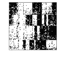
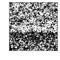
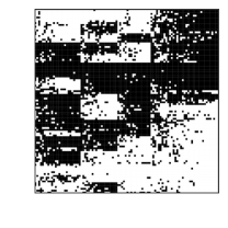
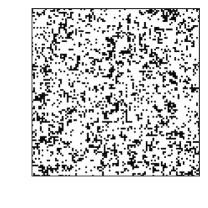
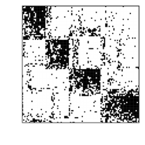
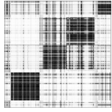
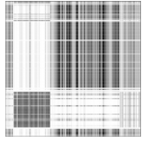
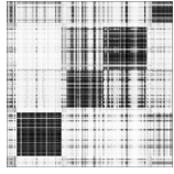
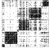
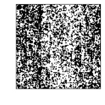
Note that each element wfksubscript𝑤𝑓𝑘w_{fk} and hknsubscript𝑘𝑛h_{kn} can be interpreted as a probability. We can either merely impose that the elements of a row 𝐰fsubscript𝐰𝑓\mathbf{w}_{f} or a column 𝐡nsubscript𝐡𝑛\mathbf{h}_{n} lie between 00 and 111, or, more strongly, that they sum up to one. This implies a difference in modeling. On the one hand, imposing that the elements lie between 00 and 111 induce non-exclusive components. On the other hand, the sum-to-one constraint induces exclusive components, i.e., the more likely a component is, the less likely are the others. Fig. 2 displays simulated matrices generated from each of the models.
Refer to caption
Refer to caption
(a) Beta-Dir
Refer to caption
Refer to caption
(b) Dir-Beta
Refer to caption
Refer to caption
(c) Dir-Dir
Figure 2: Synthetic 100×100100100100\times 100 matrices drawn from the three generative models with K=4𝐾4K=4. Matrices on the left are generated with αk=βk=γk=ηk=1subscript𝛼𝑘subscript𝛽𝑘subscript𝛾𝑘subscript𝜂𝑘1\alpha_{k}=\beta_{k}=\gamma_{k}=\eta_{k}=1. Matrices on the right are generated with αk=βk=γk=ηk=0.1subscript𝛼𝑘subscript𝛽𝑘subscript𝛾𝑘subscript𝜂𝑘0.1\alpha_{k}=\beta_{k}=\gamma_{k}=\eta_{k}=0.1. For better visualization, rows and columns are re-ordered according to complete linkage clustering (Sørensen, 1948) using the hclust function in R (R Core Team, 2017).

The first two models, Beta-Dir and Dir-Beta, are symmetric. Indeed, estimating 𝐖𝐖\mathbf{W} (resp., 𝐇𝐇\mathbf{H}) in one model is equivalent to estimating 𝐇𝐇\mathbf{H} (resp., 𝐖𝐖\mathbf{W}) in the other model after transposing the matrix 𝐕𝐕\mathbf{V}. As such, in the rest of the paper, we will only consider the Beta-Dir model and the Dir-Dir model.

The Aspect Bernoulli model of Bingham et al. (2009) is built over Eq. (11), and considers that the factors 𝐖𝐖\mathbf{W} and 𝐇𝐇\mathbf{H} are deterministic parameters which satisfy the constraint (c2). The factors are estimated by maximum likelihood with EM. The binary ICA of Kabán and Bingham (2008) corresponds to the Beta-Dir model, and inference is performed with VB. In the following sections, we present inference methods for the posterior distributions of 𝐖𝐖\mathbf{W} and 𝐇𝐇\mathbf{H} in the Beta-Dir and Dir-Dir models. Because these distributions are intractable, we propose novel collapsed Gibbs sampling and collapsed variational inference strategies. We also derive a nonparametric approximation where the number of latent dimensions K𝐾K does not need to be fixed a priori.

3.2 Connections with latent Dirichlet allocation (LDA).

The proposed models have connection with topic models, in particular with LDA (Blei et al., 2003), described by

𝐡nsubscript𝐡𝑛\displaystyle\mathbf{h}_{n} Dirichlet(𝜸)similar-toabsentDirichlet𝜸\displaystyle\sim\text{Dirichlet}(\boldsymbol{\mathbf{\gamma}}) (12)
𝐯n|𝐡nconditionalsubscript𝐯𝑛subscript𝐡𝑛\displaystyle\mathbf{v}_{n}|\mathbf{h}_{n} Multinomial(Ln,𝐖𝐡n).similar-toabsentMultinomialsubscript𝐿𝑛subscript𝐖𝐡𝑛\displaystyle\sim{\text{Multinomial}\left(L_{n},{\mathbf{W}}{\mathbf{h}}_{n}\right)}. (13)

Here, 𝐕𝐕\mathbf{V} is the so-called “bag-of-words” representation of a corpus of documents, i.e., vfnsubscript𝑣𝑓𝑛v_{fn} represents the number of occurrences of word f𝑓f in document n𝑛n. Lnsubscript𝐿𝑛L_{n} is the total number of words in document n𝑛n, i.e., Ln=fvfnsubscript𝐿𝑛subscript𝑓subscript𝑣𝑓𝑛L_{n}=\sum_{f}v_{fn}. The columns of 𝐖𝐖\mathbf{W} are assumed to sum to 1, such that wfksubscript𝑤𝑓𝑘w_{fk} represents the probability of word f𝑓f in topic k𝑘k, and hknsubscript𝑘𝑛h_{kn} represents the probability of topic k𝑘k in document n𝑛n. In standard LDA, no prior distribution is assumed on 𝐖𝐖\mathbf{W}, though it is common practice to assume Dirichlet distributions column-wise. The observation model is multinomial, with a total “budget” of Lnsubscript𝐿𝑛L_{n} words to distribute in each document n𝑛n. In contrast, the binary data models presented in this article are based on independent Bernoulli observations, and cannot be recast as multinomial. An LDA-like model may arise if we assume that each column of 𝐕𝐕\mathbf{V} contains only one 1, and the rest are zeros (i.e. Ln=1subscript𝐿𝑛1L_{n}=1 for all n𝑛n). This setting is however not considered in the article.

3.3 Bayesian inference

In this paper, we opt for Bayesian inference of the latent factors 𝐖𝐖{\mathbf{W}} and 𝐇𝐇{\mathbf{H}}. This means that we seek to characterize the posterior distribution p(𝐖,𝐇|𝐕)𝑝𝐖conditional𝐇𝐕p({\mathbf{W}},{\mathbf{H}}|{\mathbf{V}}). The posterior in the considered models is not available in closed form and we will resort to numerical approximations (Markov Chain Monte Carlo sampling, variational inference). Another possible route is to seek point estimates through either constrained maximum likelihood (ML) or maximum a posteriori (MAP) estimation. For example, given Eq. (11) and the set of constraints (c1), maximum likelihood estimation writes

min𝐖,𝐇logp(𝐕|𝐖𝐇)=f,nvfnlog([𝐖𝐇]fn)+(1vfn)log(1[𝐖𝐇]fn)subscript𝐖𝐇𝑝conditional𝐕𝐖𝐇subscript𝑓𝑛subscript𝑣𝑓𝑛subscriptdelimited-[]𝐖𝐇𝑓𝑛1subscript𝑣𝑓𝑛1subscriptdelimited-[]𝐖𝐇𝑓𝑛\displaystyle\min_{\mathbf{W},\mathbf{H}}-\log p(\mathbf{V}|\mathbf{W}\mathbf{H})=\sum_{f,n}v_{fn}\log([{\mathbf{W}}{\mathbf{H}}]_{fn})+(1-v_{fn})\log(1-[{\mathbf{W}}{\mathbf{H}}]_{fn})
subject to(1)wfk,hkn0,(2)kwfk=1,(3)hkn[0,1].formulae-sequencesubject to1subscript𝑤𝑓𝑘subscript𝑘𝑛0formulae-sequence2subscript𝑘subscript𝑤𝑓𝑘13subscript𝑘𝑛01\displaystyle\text{subject to}\quad(1)\ w_{fk},h_{kn}\geq 0,\quad(2)\ \sum_{k}w_{fk}=1,\quad(3)\ h_{kn}\in[0,1]. (14)

Such optimization problems may be tackled with, e.g., majorization-minimization (Bingham et al., 2009) or proximal gradient descent (Udell et al., 2016). Though it can be computationally more costly, we favored Bayesian inference for the following reasons. Characterizing the full posterior provides a measure of uncertainty over the latent parameters and over predicted values of 𝐕𝐕{\mathbf{V}}. As we will show later, it allows in turn to infer the rank K𝐾K of the factorization, a very desirable property that is more difficult to obtain with point estimation methods. Finally, Bayesian inference is rather customary in topic models such as LDA or Discrete Component Analysis (Buntine and Jakulin, 2006), and our work intends to follow similar principles.

4 Inference in the Beta-Dir model

In this section, we derive a collapsed Gibbs sampler (Liu, 1994) for the Beta-Dir model. First, we will augment the model with latent indicator variables 𝐙𝐙\boldsymbol{\mathbf{Z}} so that it becomes conjugate. Then the collapsed Gibbs sampler consists in marginalizing out the factors 𝐖𝐖\boldsymbol{\mathbf{W}} and 𝐇𝐇\boldsymbol{\mathbf{H}}, thus running a Gibbs sampler over the indicator variables 𝐙𝐙\boldsymbol{\mathbf{Z}} only. The interest of collapsed Gibbs sampling is that it offers improved mixing properties of the Markov chains, i.e., better exploration of the parameter space, thanks to the reduced dimensionality. We use a superscript, as in x(j)superscript𝑥𝑗x^{(j)}, to indicate the j𝑗j-th sample of a chain (after burn-in). After sampling, given a collection of samples 𝐙(j)superscript𝐙𝑗\boldsymbol{\mathbf{Z}}^{(j)} from the posterior, we will be able to directly sample from the posteriors of interest p(𝐖|𝐕)𝑝conditional𝐖𝐕p(\boldsymbol{\mathbf{W}}|\boldsymbol{\mathbf{V}}) and p(𝐇|𝐕)𝑝conditional𝐇𝐕p(\boldsymbol{\mathbf{H}}|\boldsymbol{\mathbf{V}}).

4.1 Augmented model

𝜸𝜸\boldsymbol{\mathbf{\gamma}} 𝐰fsubscript𝐰𝑓\boldsymbol{\mathbf{w}}_{f} 𝐳fnsubscript𝐳𝑓𝑛\boldsymbol{\mathbf{z}}_{fn}vfnsubscript𝑣𝑓𝑛v_{fn} hknsubscript𝑘𝑛h_{kn}αksubscript𝛼𝑘\alpha_{k}βksubscript𝛽𝑘\beta_{k}F𝐹FN𝑁NK𝐾K
(a) Partially augmented Beta-Dir model
𝜸𝜸\boldsymbol{\mathbf{\gamma}} 𝐰fsubscript𝐰𝑓\boldsymbol{\mathbf{w}}_{f} 𝐳fnsubscript𝐳𝑓𝑛\boldsymbol{\mathbf{z}}_{fn}vfnsubscript𝑣𝑓𝑛v_{fn} 𝐜fnsubscript𝐜𝑓𝑛\boldsymbol{\mathbf{c}}_{fn}𝐡nsubscript𝐡𝑛\boldsymbol{\mathbf{h}}_{n}𝜼𝜼\boldsymbol{\mathbf{\eta}}F𝐹FN𝑁N
(b) Fully augmented Dir-Dir model
Figure 3: Augmented models

We can augment the Beta-Dir model with indicator variables 𝐳fnsubscript𝐳𝑓𝑛\boldsymbol{\mathbf{z}}_{fn}, that contain component assignments from the Dirichlet factor, as shown in Bingham et al. (2009). More precisely, 𝐳fnsubscript𝐳𝑓𝑛\boldsymbol{\mathbf{z}}_{fn} is a vector of dimension K𝐾K with elements zfkn{0,1}subscript𝑧𝑓𝑘𝑛01z_{fkn}\in\{0,1\} such that only one element equals to one and all the others equal to zero. In other words, 𝐳fn{𝐞1,,𝐞K}subscript𝐳𝑓𝑛subscript𝐞1subscript𝐞𝐾\boldsymbol{\mathbf{z}}_{fn}\in\{\boldsymbol{\mathbf{e}}_{1},\ldots,\boldsymbol{\mathbf{e}}_{K}\}, where 𝐞ksubscript𝐞𝑘\boldsymbol{\mathbf{e}}_{k} is the k𝑘k-th canonical vector of Ksuperscript𝐾\mathbb{R}^{K}. The augmented model is a mixture model described by:333Some readers may be more accustomed to the alternative notation where the “one-hot” variable 𝐳fnsubscript𝐳𝑓𝑛\boldsymbol{\mathbf{z}}_{fn} is replaced by an integer-valued index zfn{1,,K}subscript𝑧𝑓𝑛1𝐾z_{fn}\in\{1,\ldots,K\}. In this case, the Bernoulli parameter in Eq. (18) becomes hzfnnsubscriptsubscript𝑧𝑓𝑛𝑛h_{z_{fn}n}.

hknsubscript𝑘𝑛\displaystyle h_{kn} Beta(αk,βk)similar-toabsentBetasubscript𝛼𝑘subscript𝛽𝑘\displaystyle\sim\text{Beta}(\alpha_{k},\beta_{k}) (15)
𝐰fsubscript𝐰𝑓\displaystyle\boldsymbol{\mathbf{w}}_{f} Dirichlet(𝜸)similar-toabsentDirichlet𝜸\displaystyle\sim\text{Dirichlet}(\boldsymbol{\mathbf{\gamma}}) (16)
𝐳fn|𝐰fconditionalsubscript𝐳𝑓𝑛subscript𝐰𝑓\displaystyle\boldsymbol{\mathbf{z}}_{fn}|\boldsymbol{\mathbf{w}}_{f} Discrete(𝐰f)similar-toabsentDiscretesubscript𝐰𝑓\displaystyle\sim\text{Discrete}(\boldsymbol{\mathbf{w}}_{f}) (17)
vfn|𝐡n,𝐳fnconditionalsubscript𝑣𝑓𝑛subscript𝐡𝑛subscript𝐳𝑓𝑛\displaystyle v_{fn}|\boldsymbol{\mathbf{h}}_{n},\boldsymbol{\mathbf{z}}_{fn} Bernoulli(khknzfkn).similar-toabsentBernoullisubscriptproduct𝑘superscriptsubscript𝑘𝑛subscript𝑧𝑓𝑘𝑛\displaystyle\sim\text{Bernoulli}\left(\prod_{k}h_{kn}^{z_{fkn}}\right). (18)

Indeed, marginalizing 𝐳fnsubscript𝐳𝑓𝑛\boldsymbol{\mathbf{z}}_{fn} from Eqs. (17)-(18) leads to Eq. (11) as shown next. From Eqs. (17)-(18) we have

p(vfn|𝐰f,𝐡n)𝑝conditionalsubscript𝑣𝑓𝑛subscript𝐰𝑓subscript𝐡𝑛\displaystyle p(v_{fn}|{\mathbf{w}}_{f},\boldsymbol{\mathbf{h}}_{n}) =kp(𝐳fn=𝐞k|𝐰f)Bernoulli(vfn|hkn,zfkn)absentsubscript𝑘𝑝subscript𝐳𝑓𝑛conditionalsubscript𝐞𝑘subscript𝐰𝑓Bernoulliconditionalsubscript𝑣𝑓𝑛subscript𝑘𝑛subscript𝑧𝑓𝑘𝑛\displaystyle=\sum_{k}p(\boldsymbol{\mathbf{z}}_{fn}=\boldsymbol{\mathbf{e}}_{k}|\boldsymbol{\mathbf{w}}_{f})\,\text{Bernoulli}(v_{fn}|h_{kn},z_{fkn}) (19)
=kwfkhknvfn(1hkn)1vfn,absentsubscript𝑘subscript𝑤𝑓𝑘superscriptsubscript𝑘𝑛subscript𝑣𝑓𝑛superscript1subscript𝑘𝑛1subscript𝑣𝑓𝑛\displaystyle=\sum_{k}w_{fk}\,h_{kn}^{v_{fn}}(1-h_{kn})^{1-v_{fn}}, (20)

and thus p(vfn=1|𝐰f,𝐡n)=[𝐖𝐇]fn𝑝subscript𝑣𝑓𝑛conditional1subscript𝐰𝑓subscript𝐡𝑛subscriptdelimited-[]𝐖𝐇𝑓𝑛p(v_{fn}=1|{\mathbf{w}}_{f},\boldsymbol{\mathbf{h}}_{n})=[\boldsymbol{\mathbf{W}}\boldsymbol{\mathbf{H}}]_{fn} and p(vfn=0|𝐰f,𝐡n)=1[𝐖𝐇]fn𝑝subscript𝑣𝑓𝑛conditional0subscript𝐰𝑓subscript𝐡𝑛1subscriptdelimited-[]𝐖𝐇𝑓𝑛p(v_{fn}=0|{\mathbf{w}}_{f},\boldsymbol{\mathbf{h}}_{n})=1-[\boldsymbol{\mathbf{W}}\boldsymbol{\mathbf{H}}]_{fn}, i.e., vfnsubscript𝑣𝑓𝑛v_{fn} has the marginal distribution given by Eq. (11). A graphical representation of the augmented model is shown in Fig. 3-(a). Let us think of a recommender system application, where columns of 𝐕𝐕\boldsymbol{\mathbf{V}} are users, and rows are items. An interpretation of the above model is the following. Each item f𝑓f is characterized by a probability over topics, 𝐰fsubscript𝐰𝑓\boldsymbol{\mathbf{w}}_{f}. Then, for each user-item pair, a topic k𝑘k (indicated by 𝐳fnsubscript𝐳𝑓𝑛\boldsymbol{\mathbf{z}}_{fn}) is activated with probability wfksubscript𝑤𝑓𝑘w_{fk}, and the probability that the user n𝑛n consumes this item (vfn=1subscript𝑣𝑓𝑛1v_{fn}=1) is hknsubscript𝑘𝑛h_{kn}.

Denoting by 𝐙𝐙\mathbf{Z} the F×K×N𝐹𝐾𝑁F\times K\times N tensor with entries zfknsubscript𝑧𝑓𝑘𝑛z_{fkn}, the joint probability in the augmented model is given by:

p(𝐕,𝐙,𝐖,𝐇)=p(𝐖)p(𝐙|𝐖)p(𝐇)p(𝐕|𝐇,𝐙)=𝑝𝐕𝐙𝐖𝐇𝑝𝐖𝑝conditional𝐙𝐖𝑝𝐇𝑝conditional𝐕𝐇𝐙absent\displaystyle p(\boldsymbol{\mathbf{V}},\boldsymbol{\mathbf{Z}},\boldsymbol{\mathbf{W}},\boldsymbol{\mathbf{H}})=p(\boldsymbol{\mathbf{W}})p(\boldsymbol{\mathbf{Z}}|\boldsymbol{\mathbf{W}})p(\boldsymbol{\mathbf{H}})p(\boldsymbol{\mathbf{V}}|\boldsymbol{\mathbf{H}},\boldsymbol{\mathbf{Z}})=
[f=1F(p(𝐰f)n=1Np(𝐳fn|𝐰f))][n=1N(k=1Kp(hkn)f=1Fp(vfn|𝐡n,𝐳fn))].delimited-[]superscriptsubscriptproduct𝑓1𝐹𝑝subscript𝐰𝑓superscriptsubscriptproduct𝑛1𝑁𝑝conditionalsubscript𝐳𝑓𝑛subscript𝐰𝑓delimited-[]superscriptsubscriptproduct𝑛1𝑁superscriptsubscriptproduct𝑘1𝐾𝑝subscript𝑘𝑛superscriptsubscriptproduct𝑓1𝐹𝑝conditionalsubscript𝑣𝑓𝑛subscript𝐡𝑛subscript𝐳𝑓𝑛\displaystyle\left[\prod_{f=1}^{F}\left(p(\boldsymbol{\mathbf{w}}_{f})\prod_{n=1}^{N}p(\boldsymbol{\mathbf{z}}_{fn}|\boldsymbol{\mathbf{w}}_{f})\right)\right]\left[\prod_{n=1}^{N}\left(\prod_{k=1}^{K}p(h_{kn})\prod_{f=1}^{F}p(v_{fn}|\boldsymbol{\mathbf{h}}_{n},\boldsymbol{\mathbf{z}}_{fn})\right)\right]. (21)

4.2 Collapsed Gibbs sampler

Thanks to the previous augmentation, and exploiting conjugacy, we can now marginalize out 𝐖𝐖\boldsymbol{\mathbf{W}} and 𝐇𝐇\boldsymbol{\mathbf{H}} from Eq. (21). The marginalized distribution has the following structure:

p(𝐕,𝐙)=𝑝𝐕𝐙absent\displaystyle p(\mathbf{V},\mathbf{Z})=
fp(𝐰f)np(𝐳fn|𝐰f)d𝐰fp(𝐙¯f)nkp(hkn)fp(vfn|𝐡n,𝐳fn)d𝐡np(𝐯n|𝐙n),subscriptproduct𝑓superscript𝑝subscript𝐰𝑓subscriptproduct𝑛𝑝conditionalsubscript𝐳𝑓𝑛subscript𝐰𝑓𝑑subscript𝐰𝑓𝑝subscript¯𝐙𝑓subscriptproduct𝑛superscriptsubscriptproduct𝑘𝑝subscript𝑘𝑛subscriptproduct𝑓𝑝conditionalsubscript𝑣𝑓𝑛subscript𝐡𝑛subscript𝐳𝑓𝑛𝑑subscript𝐡𝑛𝑝conditionalsubscript𝐯𝑛subscript𝐙𝑛\displaystyle\prod_{f}\overbrace{\int p(\boldsymbol{\mathbf{w}}_{f})\prod_{n}p(\boldsymbol{\mathbf{z}}_{fn}|\boldsymbol{\mathbf{w}}_{f})\,d\mathbf{w}_{f}}^{p(\underline{\boldsymbol{\mathbf{Z}}}_{f})}\prod_{n}\overbrace{\int\prod_{k}p(h_{kn})\prod_{f}p(v_{fn}|\boldsymbol{\mathbf{h}}_{n},\boldsymbol{\mathbf{z}}_{fn})\,d{\mathbf{h}}_{n}}^{p(\boldsymbol{\mathbf{v}}_{n}|\boldsymbol{\mathbf{Z}}_{n})}, (22)

where 𝐙¯fsubscript¯𝐙𝑓\underline{\mathbf{Z}}_{f} denotes the K×N𝐾𝑁K\times N matrix with entries {zfkn}knsubscriptsubscript𝑧𝑓𝑘𝑛𝑘𝑛\{z_{fkn}\}_{kn}, 𝐙nsubscript𝐙𝑛\mathbf{Z}_{n} denotes the F×K𝐹𝐾F\times K matrix with entries {zfkn}fksubscriptsubscript𝑧𝑓𝑘𝑛𝑓𝑘\{z_{fkn}\}_{fk}. Let us define the following four variables that act as counters:

Lfksubscript𝐿𝑓𝑘\displaystyle L_{fk} =nzfkn,absentsubscript𝑛subscript𝑧𝑓𝑘𝑛\displaystyle=\sum_{n}z_{fkn}, Mknsubscript𝑀𝑘𝑛\displaystyle M_{kn} =fzfkn,absentsubscript𝑓subscript𝑧𝑓𝑘𝑛\displaystyle=\sum_{f}z_{fkn},
Aknsubscript𝐴𝑘𝑛\displaystyle A_{kn} =fzfknvfn,absentsubscript𝑓subscript𝑧𝑓𝑘𝑛subscript𝑣𝑓𝑛\displaystyle=\sum_{f}z_{fkn}v_{fn}, Bknsubscript𝐵𝑘𝑛\displaystyle B_{kn} =fzfknv¯fn.absentsubscript𝑓subscript𝑧𝑓𝑘𝑛subscript¯𝑣𝑓𝑛\displaystyle=\sum_{f}z_{fkn}\bar{v}_{fn}.

where v¯fn=1vfnsubscript¯𝑣𝑓𝑛1subscript𝑣𝑓𝑛\bar{v}_{fn}=1-v_{fn}. Aknsubscript𝐴𝑘𝑛A_{kn} and Bknsubscript𝐵𝑘𝑛B_{kn} count how many times the component k𝑘k is associated to a “positive” observation (vfn=1subscript𝑣𝑓𝑛1v_{fn}=1) and to a “negative” observation (v¯fn=1subscript¯𝑣𝑓𝑛1\bar{v}_{fn}=1) in the n𝑛n-th sample. Then we have the following expressions (derivations are available in Appendix B.1):

p(𝐙¯f)𝑝subscript¯𝐙𝑓\displaystyle p(\underline{\boldsymbol{\mathbf{Z}}}_{f}) =Γ(kγk)kΓ(γk)kΓ(γk+Lfk)Γ(kγk+N)absentΓsubscript𝑘subscript𝛾𝑘subscriptproduct𝑘Γsubscript𝛾𝑘subscriptproduct𝑘Γsubscript𝛾𝑘subscript𝐿𝑓𝑘Γsubscript𝑘subscript𝛾𝑘𝑁\displaystyle=\frac{\Gamma(\sum_{k}\gamma_{k})}{\prod_{k}\Gamma(\gamma_{k})}\frac{\prod_{k}\Gamma(\gamma_{k}+L_{fk})}{\Gamma(\sum_{k}\gamma_{k}+N)} (23)
p(𝐯n|𝐙n)𝑝conditionalsubscript𝐯𝑛subscript𝐙𝑛\displaystyle p(\boldsymbol{\mathbf{v}}_{n}|\boldsymbol{\mathbf{Z}}_{n}) =kΓ(αk+βk)Γ(αk)Γ(βk)Γ(αk+Akn)Γ(βk+Bkn)Γ(αk+βk+Mkn).absentsubscriptproduct𝑘Γsubscript𝛼𝑘subscript𝛽𝑘Γsubscript𝛼𝑘Γsubscript𝛽𝑘Γsubscript𝛼𝑘subscript𝐴𝑘𝑛Γsubscript𝛽𝑘subscript𝐵𝑘𝑛Γsubscript𝛼𝑘subscript𝛽𝑘subscript𝑀𝑘𝑛\displaystyle=\prod_{k}\frac{\Gamma(\alpha_{k}+\beta_{k})}{\Gamma(\alpha_{k})\Gamma(\beta_{k})}\frac{\Gamma(\alpha_{k}+A_{kn})\Gamma(\beta_{k}+B_{kn})}{\Gamma(\alpha_{k}+\beta_{k}+M_{kn})}. (24)

The posterior of the indicator variables p(𝐙|𝐕)𝑝conditional𝐙𝐕p(\boldsymbol{\mathbf{Z}}|\boldsymbol{\mathbf{V}}) is not available in closed form and the proposed collapsed Gibbs sampler consists in iteratively sampling each vector 𝐳fnsubscript𝐳𝑓𝑛\boldsymbol{\mathbf{z}}_{fn} given the current value of the other indicator vectors. Let Lfk¬fnsuperscriptsubscript𝐿𝑓𝑘𝑓𝑛L_{fk}^{\neg fn}, Mkn¬fnsuperscriptsubscript𝑀𝑘𝑛𝑓𝑛M_{kn}^{\neg fn}, Akn¬fnsuperscriptsubscript𝐴𝑘𝑛𝑓𝑛A_{kn}^{\neg fn}, Bkn¬fnsuperscriptsubscript𝐵𝑘𝑛𝑓𝑛B_{kn}^{\neg fn} be the state of the counters when the tube (f,n)𝑓𝑛(f,n) of the tensor 𝐙𝐙\boldsymbol{\mathbf{Z}} is left out of the sums:

Lfk¬fnsuperscriptsubscript𝐿𝑓𝑘𝑓𝑛\displaystyle L_{fk}^{\neg fn} =Lfkzfkn,absentsubscript𝐿𝑓𝑘subscript𝑧𝑓𝑘𝑛\displaystyle=L_{fk}-z_{fkn}, Mkn¬fnsuperscriptsubscript𝑀𝑘𝑛𝑓𝑛\displaystyle M_{kn}^{\neg fn} =Mknzfkn,absentsubscript𝑀𝑘𝑛subscript𝑧𝑓𝑘𝑛\displaystyle=M_{kn}-z_{fkn},
Akn¬fnsuperscriptsubscript𝐴𝑘𝑛𝑓𝑛\displaystyle A_{kn}^{\neg fn} =Aknzfknvfn,absentsubscript𝐴𝑘𝑛subscript𝑧𝑓𝑘𝑛subscript𝑣𝑓𝑛\displaystyle=A_{kn}-z_{fkn}v_{fn}, Bkn¬fnsuperscriptsubscript𝐵𝑘𝑛𝑓𝑛\displaystyle B_{kn}^{\neg fn} =Bknzfknv¯fn.absentsubscript𝐵𝑘𝑛subscript𝑧𝑓𝑘𝑛subscript¯𝑣𝑓𝑛\displaystyle=B_{kn}-z_{fkn}\bar{v}_{fn}.

In Appendix B.2 we show that the conditional posterior of 𝐳fnsubscript𝐳𝑓𝑛\boldsymbol{\mathbf{z}}_{fn} given the remaining variables 𝐙¬fnsubscript𝐙𝑓𝑛\boldsymbol{\mathbf{Z}}_{\neg fn} is given by:

p(𝐳fn|𝐙¬fn,𝐕)k[(γk+Lfk¬fn)(αk+Akn¬fn)vfn(βk+Bkn¬fn)v¯fnαk+βk+Mkn¬fn]zfkn.proportional-to𝑝conditionalsubscript𝐳𝑓𝑛subscript𝐙𝑓𝑛𝐕subscriptproduct𝑘superscriptdelimited-[]subscript𝛾𝑘superscriptsubscript𝐿𝑓𝑘𝑓𝑛superscriptsubscript𝛼𝑘superscriptsubscript𝐴𝑘𝑛𝑓𝑛subscript𝑣𝑓𝑛superscriptsubscript𝛽𝑘superscriptsubscript𝐵𝑘𝑛𝑓𝑛subscript¯𝑣𝑓𝑛subscript𝛼𝑘subscript𝛽𝑘superscriptsubscript𝑀𝑘𝑛𝑓𝑛subscript𝑧𝑓𝑘𝑛\displaystyle p(\boldsymbol{\mathbf{z}}_{fn}|\boldsymbol{\mathbf{Z}}_{\neg fn},\boldsymbol{\mathbf{V}})\propto\prod_{k}\left[(\gamma_{k}+L_{fk}^{\neg fn})\frac{(\alpha_{k}+A_{kn}^{\neg fn})^{v_{fn}}(\beta_{k}+B_{kn}^{\neg fn})^{\bar{v}_{fn}}}{\alpha_{k}+\beta_{k}+M_{kn}^{\neg fn}}\right]^{z_{fkn}}. (25)

This expression needs to be normalized to ensure a valid probability distribution. This can be easily done by computing the right-hand side of Eq. (25) for every of the K𝐾K possible values of 𝐳fnsubscript𝐳𝑓𝑛\boldsymbol{\mathbf{z}}_{fn} and normalizing by the sum. Eq. (25) shows that the probability of choosing a component k𝑘k depends on the number of elements already assigned to that component. More precisely, it depends on the one hand on the number of elements assigned to component k𝑘k in column n𝑛n. On the other hand, it also depends on the proportion of elements in row f𝑓f assigned to component k𝑘k that explain ones (if vfn=1subscript𝑣𝑓𝑛1v_{fn}=1) or zeros (if vfn=0subscript𝑣𝑓𝑛0v_{fn}=0) in 𝐕𝐕\boldsymbol{\mathbf{V}} in the total number of elements associated to k𝑘k in that row (see Figure 4). The parameters γk,αk,βksubscript𝛾𝑘subscript𝛼𝑘subscript𝛽𝑘\gamma_{k},\alpha_{k},\beta_{k} act as pseudo-counts: they give a priori belief about how many elements are assigned to each component.

(\left(\vbox{\hrule height=32.10233pt,depth=32.10233pt,width=0.0pt}\right.)\left.\vbox{\hrule height=32.10233pt,depth=32.10233pt,width=0.0pt}\right)𝐕𝐕\boldsymbol{\mathbf{V}}
(a) Observed matrix
(\left(\vbox{\hrule height=34.50235pt,depth=34.50235pt,width=0.0pt}\right.)\left.\vbox{\hrule height=34.50235pt,depth=34.50235pt,width=0.0pt}\right)𝐙𝐙\boldsymbol{\mathbf{Z}}
(b) Beta-Dir
(\left(\vbox{\hrule height=32.70233pt,depth=32.70233pt,width=0.0pt}\right.)\left.\vbox{\hrule height=32.70233pt,depth=32.70233pt,width=0.0pt}\right)𝐙𝐙\boldsymbol{\mathbf{Z}}(\left(\vbox{\hrule height=35.01993pt,depth=35.01993pt,width=0.0pt}\right.)\left.\vbox{\hrule height=35.01993pt,depth=35.01993pt,width=0.0pt}\right)𝐂𝐂\boldsymbol{\mathbf{C}}
(c) Dir-Dir
Figure 4: Illustration of the Gibbs samplers. Colors represent component assignments (a value of k𝑘k). When sampling an element (dashed circle) the probability of each component depends on the number of elements with thick circles in the same row or column that are currently assigned to that component.

Our collapsed Gibbs sampling is summarized in Alg. (1). Note that, although Alg. (1) does not explicitly include it, we must draw samples during an initial burn-in phase (as required by any MCMC method) before collecting the last J𝐽J samples, after the chain has converged to the stationary distribution. Note also that the algorithm can readily deal with incomplete matrices by simply skipping missing entries (i.e., the loop over f𝑓f and n𝑛n only runs over available entries).

Input: Observed matrix 𝐕{0,1}F×N𝐕superscript01𝐹𝑁\boldsymbol{\mathbf{V}}\in\{0,1\}^{F\times N}
Parameters: 𝜶,𝜷,𝜸𝜶𝜷𝜸\boldsymbol{\mathbf{\alpha}},\boldsymbol{\mathbf{\beta}},\boldsymbol{\mathbf{\gamma}}
Output: Samples 𝐙(1),,𝐙(J)superscript𝐙1superscript𝐙𝐽\boldsymbol{\mathbf{Z}}^{(1)},...,\boldsymbol{\mathbf{Z}}^{(J)}
Initialize: Random initialization of 𝐙𝐙\boldsymbol{\mathbf{Z}}
for j=1𝑗1j=1 to J𝐽J  do
       for f=1𝑓1f=1 to F𝐹F  do
             for n=1𝑛1n=1 to N𝑁N  do
                   if vfnsubscript𝑣𝑓𝑛v_{fn} not missing then
                         Sample 𝐳fn(j)p(𝐳fn|𝐙¬fn,𝐕)similar-tosuperscriptsubscript𝐳𝑓𝑛𝑗𝑝conditionalsubscript𝐳𝑓𝑛subscript𝐙𝑓𝑛𝐕\boldsymbol{\mathbf{z}}_{fn}^{(j)}\sim p(\boldsymbol{\mathbf{z}}_{fn}|\boldsymbol{\mathbf{Z}}_{\neg fn},\boldsymbol{\mathbf{V}}) (Eq.(25))
                   end if
                  
             end for
            
       end for
      
end for
Algorithm 1 Collapsed Gibbs sampler for Beta-Dir

Latent factors posteriors. Thanks to conjugacy, the conditional posteriors of 𝐖𝐖\mathbf{W} and 𝐇𝐇\mathbf{H} given 𝐙𝐙\boldsymbol{\mathbf{Z}} and 𝐕𝐕\boldsymbol{\mathbf{V}} are given by:

𝐰f|𝐙¯fconditionalsubscript𝐰𝑓subscript¯𝐙𝑓\displaystyle\boldsymbol{\mathbf{w}}_{f}|\underline{\boldsymbol{\mathbf{Z}}}_{f} Dirichlet(𝜸+n𝐳fn)similar-toabsentDirichlet𝜸subscript𝑛subscript𝐳𝑓𝑛\displaystyle\sim\text{Dirichlet}(\boldsymbol{\mathbf{\gamma}}+\sum_{n}\boldsymbol{\mathbf{z}}_{fn}) (26)
hkn|𝐙n,𝐯nconditionalsubscript𝑘𝑛subscript𝐙𝑛subscript𝐯𝑛\displaystyle h_{kn}|\boldsymbol{\mathbf{Z}}_{n},\boldsymbol{\mathbf{v}}_{n} Beta(αk+Akn,βk+Bkn).similar-toabsentBetasubscript𝛼𝑘subscript𝐴𝑘𝑛subscript𝛽𝑘subscript𝐵𝑘𝑛\displaystyle\sim\text{Beta}(\alpha_{k}+A_{kn},~{}\beta_{k}+B_{kn}). (27)

The conditional posterior expectations are given by:

𝔼𝐰f[𝐰f|𝐙¯f]subscript𝔼subscript𝐰𝑓delimited-[]conditionalsubscript𝐰𝑓subscript¯𝐙𝑓\displaystyle\mathbb{E}_{\boldsymbol{\mathbf{w}}_{f}}[\boldsymbol{\mathbf{w}}_{f}|\underline{\boldsymbol{\mathbf{Z}}}_{f}] =𝜸+n𝐳fnkγk+knzfkn=𝜸+n𝐳fnkγk+Nabsent𝜸subscript𝑛subscript𝐳𝑓𝑛subscript𝑘subscript𝛾𝑘subscript𝑘subscript𝑛subscript𝑧𝑓𝑘𝑛𝜸subscript𝑛subscript𝐳𝑓𝑛subscript𝑘subscript𝛾𝑘𝑁\displaystyle=\frac{\boldsymbol{\mathbf{\gamma}}+\sum_{n}\boldsymbol{\mathbf{z}}_{fn}}{\sum_{k}\gamma_{k}+\sum_{k}\sum_{n}z_{fkn}}=\frac{\boldsymbol{\mathbf{\gamma}}+\sum_{n}\boldsymbol{\mathbf{z}}_{fn}}{\sum_{k}\gamma_{k}+N} (28)
𝔼hkn[hkn|𝐙n,𝐯n]subscript𝔼subscript𝑘𝑛delimited-[]conditionalsubscript𝑘𝑛subscript𝐙𝑛subscript𝐯𝑛\displaystyle\mathbb{E}_{h_{kn}}[h_{kn}|\boldsymbol{\mathbf{Z}}_{n},\boldsymbol{\mathbf{v}}_{n}] =αk+Aknαk+Akn+βk+Bkn=αk+fzfknvfnαk+βk+fzfkn,absentsubscript𝛼𝑘subscript𝐴𝑘𝑛subscript𝛼𝑘subscript𝐴𝑘𝑛subscript𝛽𝑘subscript𝐵𝑘𝑛subscript𝛼𝑘subscript𝑓subscript𝑧𝑓𝑘𝑛subscript𝑣𝑓𝑛subscript𝛼𝑘subscript𝛽𝑘subscript𝑓subscript𝑧𝑓𝑘𝑛\displaystyle=\frac{\alpha_{k}+A_{kn}}{\alpha_{k}+A_{kn}+\beta_{k}+B_{kn}}=\frac{\alpha_{k}+\sum_{f}z_{fkn}v_{fn}}{\alpha_{k}+\beta_{k}+\sum_{f}z_{fkn}}, (29)

where we used the equalities knzfkn=Nsubscript𝑘𝑛subscript𝑧𝑓𝑘𝑛𝑁\sum_{kn}z_{fkn}=N and Akn+Bkn=fzfknsubscript𝐴𝑘𝑛subscript𝐵𝑘𝑛subscript𝑓subscript𝑧𝑓𝑘𝑛A_{kn}+B_{kn}=\sum_{f}z_{fkn}. Using the law of total expectation, i.e., 𝔼[X]=𝔼Y[𝔼X[X|Y]]𝔼delimited-[]𝑋subscript𝔼𝑌delimited-[]subscript𝔼𝑋delimited-[]conditional𝑋𝑌\mathbb{E}[X]~{}=~{}\mathbb{E}_{Y}[\mathbb{E}_{X}[X|Y]], and given a set a samples 𝐙(j)superscript𝐙𝑗\boldsymbol{\mathbf{Z}}^{(j)}, it follows that the marginal posterior expectations of the latent factors can be computed as:

𝔼𝐰f[𝐰f|𝐕]subscript𝔼subscript𝐰𝑓delimited-[]conditionalsubscript𝐰𝑓𝐕\displaystyle\mathbb{E}_{\boldsymbol{\mathbf{w}}_{f}}[\boldsymbol{\mathbf{w}}_{f}|\boldsymbol{\mathbf{V}}] =𝔼𝐙[𝔼𝐰f[𝐰f|𝐕,𝐙]]=𝔼𝐙¯f[𝔼𝐰f[𝐰f|𝐙¯f]]𝜸+1Jjn𝐳fn(j)kγk+Nabsentsubscript𝔼𝐙delimited-[]subscript𝔼subscript𝐰𝑓delimited-[]conditionalsubscript𝐰𝑓𝐕𝐙subscript𝔼subscript¯𝐙𝑓delimited-[]subscript𝔼subscript𝐰𝑓delimited-[]conditionalsubscript𝐰𝑓subscript¯𝐙𝑓𝜸1𝐽subscript𝑗subscript𝑛superscriptsubscript𝐳𝑓𝑛𝑗subscript𝑘subscript𝛾𝑘𝑁\displaystyle=\mathbb{E}_{\boldsymbol{\mathbf{Z}}}[\mathbb{E}_{\boldsymbol{\mathbf{w}}_{f}}[\boldsymbol{\mathbf{w}}_{f}|\boldsymbol{\mathbf{V}},\boldsymbol{\mathbf{Z}}]]=\mathbb{E}_{\underline{\boldsymbol{\mathbf{Z}}}_{f}}[\mathbb{E}_{\boldsymbol{\mathbf{w}}_{f}}[\boldsymbol{\mathbf{w}}_{f}|\underline{\boldsymbol{\mathbf{Z}}}_{f}]]\approx\frac{\boldsymbol{\mathbf{\gamma}}+\frac{1}{J}\sum_{j}\sum_{n}\mathbf{z}_{fn}^{(j)}}{\sum_{k}\gamma_{k}+N} (30)
𝔼hkn[hkn|𝐕]subscript𝔼subscript𝑘𝑛delimited-[]conditionalsubscript𝑘𝑛𝐕\displaystyle\mathbb{E}_{h_{kn}}[h_{kn}|\boldsymbol{\mathbf{V}}] =𝔼𝐙n[𝔼hkn[hkn|𝐙n,𝐯n]]1Jjαk+fzfkn(j)vfnαk+βk+fzfkn(j).absentsubscript𝔼subscript𝐙𝑛delimited-[]subscript𝔼subscript𝑘𝑛delimited-[]conditionalsubscript𝑘𝑛subscript𝐙𝑛subscript𝐯𝑛1𝐽subscript𝑗subscript𝛼𝑘subscript𝑓superscriptsubscript𝑧𝑓𝑘𝑛𝑗subscript𝑣𝑓𝑛subscript𝛼𝑘subscript𝛽𝑘subscript𝑓superscriptsubscript𝑧𝑓𝑘𝑛𝑗\displaystyle=\mathbb{E}_{\boldsymbol{\mathbf{Z}}_{n}}[\mathbb{E}_{h_{kn}}[h_{kn}|\boldsymbol{\mathbf{Z}}_{n},\boldsymbol{\mathbf{v}}_{n}]]\approx\frac{1}{J}\sum_{j}\frac{\alpha_{k}+\sum_{f}z_{fkn}^{(j)}v_{fn}}{\alpha_{k}+\beta_{k}+\sum_{f}z_{fkn}^{(j)}}. (31)

Prediction. The predictive posterior distribution of an unseen data sample vfnsuperscriptsubscript𝑣𝑓𝑛v_{fn}^{*} given the available data 𝐕𝐕\boldsymbol{\mathbf{V}} is given by

p(vfn|𝐕)𝑝conditionalsuperscriptsubscript𝑣𝑓𝑛𝐕\displaystyle p(v_{fn}^{*}|\boldsymbol{\mathbf{V}}) =p(vfn|𝐰f,𝐡n)p(𝐰f,𝐡n|𝐕)𝑑𝐰f𝑑𝐡nabsent𝑝conditionalsuperscriptsubscript𝑣𝑓𝑛subscript𝐰𝑓subscript𝐡𝑛𝑝subscript𝐰𝑓conditionalsubscript𝐡𝑛𝐕differential-dsubscript𝐰𝑓differential-dsubscript𝐡𝑛\displaystyle=\int p(v_{fn}^{*}|\boldsymbol{\mathbf{w}}_{f},\boldsymbol{\mathbf{h}}_{n})p(\boldsymbol{\mathbf{w}}_{f},\boldsymbol{\mathbf{h}}_{n}|\boldsymbol{\mathbf{V}})\,d\boldsymbol{\mathbf{w}}_{f}d\boldsymbol{\mathbf{h}}_{n}
=𝔼[𝐰f𝐡n|𝐕]vfn(1𝔼[𝐰f𝐡n|𝐕])1vfn.absent𝔼superscriptdelimited-[]conditionalsubscript𝐰𝑓subscript𝐡𝑛𝐕superscriptsubscript𝑣𝑓𝑛superscript1𝔼delimited-[]conditionalsubscript𝐰𝑓subscript𝐡𝑛𝐕1superscriptsubscript𝑣𝑓𝑛\displaystyle=\mathbb{E}[\boldsymbol{\mathbf{w}}_{f}\boldsymbol{\mathbf{h}}_{n}|\boldsymbol{\mathbf{V}}]^{v_{fn}^{*}}(1-\mathbb{E}[\boldsymbol{\mathbf{w}}_{f}\boldsymbol{\mathbf{h}}_{n}|\boldsymbol{\mathbf{V}}])^{1-v_{fn}^{*}}. (32)

Because the predictive posterior is a Bernoulli distribution, its expectation is given by 𝔼[𝐰f𝐡n|𝐕]𝔼delimited-[]conditionalsubscript𝐰𝑓subscript𝐡𝑛𝐕\mathbb{E}[\boldsymbol{\mathbf{w}}_{f}\boldsymbol{\mathbf{h}}_{n}|\boldsymbol{\mathbf{V}}], which can be approximated using samples 𝐖(j)superscript𝐖𝑗\boldsymbol{\mathbf{W}}^{(j)}, 𝐇(j)superscript𝐇𝑗\boldsymbol{\mathbf{H}}^{(j)} from the distributions given by Eqs. (26)-(27) given 𝐙=𝐙(j)𝐙superscript𝐙𝑗\boldsymbol{\mathbf{Z}}=\boldsymbol{\mathbf{Z}}^{(j)}:

𝔼[vfn|𝐕]=𝔼[𝐰f𝐡n|𝐕]1Jj𝐰f(j)𝐡n(j).𝔼delimited-[]conditionalsuperscriptsubscript𝑣𝑓𝑛𝐕𝔼delimited-[]conditionalsubscript𝐰𝑓subscript𝐡𝑛𝐕1𝐽subscript𝑗superscriptsubscript𝐰𝑓𝑗superscriptsubscript𝐡𝑛𝑗\displaystyle\mathbb{E}[v_{fn}^{*}|\boldsymbol{\mathbf{V}}]=\mathbb{E}[{\boldsymbol{\mathbf{w}}_{f}\boldsymbol{\mathbf{h}}_{n}}|\boldsymbol{\mathbf{V}}]\approx\frac{1}{J}\sum_{j}\boldsymbol{\mathbf{w}}_{f}^{(j)}\boldsymbol{\mathbf{h}}_{n}^{(j)}. (33)

4.3 Collapsed variational inference

Given the collapsed model of Eqs. (22)-(24) we may derive a mean-field Collapsed Variational Bayes algorithm (CVB) (Teh et al., 2007) by assuming that the posterior factorizes as q(𝐙)=fnq(𝐳fn)𝑞𝐙subscriptproduct𝑓𝑛𝑞subscript𝐳𝑓𝑛q(\boldsymbol{\mathbf{Z}})=\prod_{fn}q(\boldsymbol{\mathbf{z}}_{fn}). The key of CVB is that its free energy is a strictly better bound on the evidence than the free energy of the standard, i.e., uncollapsed, VB. We compute the CVB updates by applying the mean-field VB updates to the collapsed model:

q(𝐳fn|𝐕)exp{𝔼q(𝐙¬fn)[logp(𝐕,𝐙)]},proportional-to𝑞conditionalsubscript𝐳𝑓𝑛𝐕subscript𝔼𝑞subscript𝐙𝑓𝑛delimited-[]𝑝𝐕𝐙\displaystyle q(\boldsymbol{\mathbf{z}}_{fn}|\boldsymbol{\mathbf{V}})\propto\exp\{\mathbb{E}_{q(\boldsymbol{\mathbf{Z}}_{\neg fn})}[\log p(\boldsymbol{\mathbf{V}},\boldsymbol{\mathbf{Z}})]\}, (34)

where the expectations are taken over the variational posterior. This leads us to

q(𝐳fn|𝐕)𝑞conditionalsubscript𝐳𝑓𝑛𝐕\displaystyle q(\boldsymbol{\mathbf{z}}_{fn}|\boldsymbol{\mathbf{V}})
kexp{𝔼q[log(γk+Lfk¬fn)]𝔼q[log(αk+Akn¬fn)]vfn𝔼q[log(βk+Bkn¬fn)]v¯fn𝔼q[logMkn¬fn]}.proportional-toabsentsubscriptproduct𝑘subscript𝔼𝑞delimited-[]subscript𝛾𝑘superscriptsubscript𝐿𝑓𝑘𝑓𝑛subscript𝔼𝑞superscriptdelimited-[]subscript𝛼𝑘superscriptsubscript𝐴𝑘𝑛𝑓𝑛subscript𝑣𝑓𝑛subscript𝔼𝑞superscriptdelimited-[]subscript𝛽𝑘superscriptsubscript𝐵𝑘𝑛𝑓𝑛subscript¯𝑣𝑓𝑛subscript𝔼𝑞delimited-[]superscriptsubscript𝑀𝑘𝑛𝑓𝑛\displaystyle\propto\prod_{k}\exp\left\{\mathbb{E}_{q}[\log(\gamma_{k}+L_{fk}^{\neg fn})]\frac{\mathbb{E}_{q}[\log(\alpha_{k}+A_{kn}^{\neg fn})]^{v_{fn}}\mathbb{E}_{q}[\log(\beta_{k}+B_{kn}^{\neg fn})]^{\bar{v}_{fn}}}{\mathbb{E}_{q}[\log M_{kn}^{\neg fn}]}\right\}. (35)

The expectations of the form 𝔼q(z)[log(x+z)]subscript𝔼𝑞𝑧delimited-[]𝑥𝑧\mathbb{E}_{q(z)}[\log(x+z)] are expensive to compute. A simpler alternative is CVB0 (Asuncion et al., 2009), which uses a zero-order Taylor approximation 𝔼q(z)[log(x+z)]log(x+𝔼q(z)[z])]\mathbb{E}_{q}(z)[\log(x+z)]\approx\log(x+\mathbb{E}_{q(z)}[z])] and has been shown to give, in some cases, better inference results than CVB. Under the CVB0 version our update becomes

q(𝐳fn|𝐕)k(γk+𝔼q[Lfk¬fn])(αk+𝔼q[Akn¬fn])vfn(βk+𝔼q[Bkn¬fn])v¯fnαk+βk+𝔼q[Mkn¬fn],proportional-to𝑞conditionalsubscript𝐳𝑓𝑛𝐕subscriptproduct𝑘subscript𝛾𝑘subscript𝔼𝑞delimited-[]superscriptsubscript𝐿𝑓𝑘𝑓𝑛superscriptsubscript𝛼𝑘subscript𝔼𝑞delimited-[]superscriptsubscript𝐴𝑘𝑛𝑓𝑛subscript𝑣𝑓𝑛superscriptsubscript𝛽𝑘subscript𝔼𝑞delimited-[]superscriptsubscript𝐵𝑘𝑛𝑓𝑛subscript¯𝑣𝑓𝑛subscript𝛼𝑘subscript𝛽𝑘subscript𝔼𝑞delimited-[]superscriptsubscript𝑀𝑘𝑛𝑓𝑛\displaystyle q(\boldsymbol{\mathbf{z}}_{fn}|\boldsymbol{\mathbf{V}})\propto\prod_{k}(\gamma_{k}+\mathbb{E}_{q}[L_{fk}^{\neg fn}])\frac{(\alpha_{k}+\mathbb{E}_{q}[A_{kn}^{\neg fn}])^{v_{fn}}(\beta_{k}+\mathbb{E}_{q}[B_{kn}^{\neg fn}])^{\bar{v}_{fn}}}{\alpha_{k}+\beta_{k}+\mathbb{E}_{q}[M_{kn}^{\neg fn}]}, (36)

which has a similar structure to the collapsed Gibbs sampler in Eq. (25). Overall, the collapsed VB algorithm has the same structure as the Gibbs sampler summarized in Alg. (1). Note that when the data matrix is too large for batch processing, one can routinely resort to stochastic variational inference (Hoffman et al., 2013).

Latent factors posteriors. The variational distributions of the factors can be obtained from the uncollapsed version:

q(𝐰f)𝑞subscript𝐰𝑓\displaystyle q(\boldsymbol{\mathbf{w}}_{f}) =Dirichlet(𝜸+n𝔼q[𝐳fn])absentDirichlet𝜸subscript𝑛subscript𝔼𝑞delimited-[]subscript𝐳𝑓𝑛\displaystyle=\text{Dirichlet}(\boldsymbol{\mathbf{\gamma}}+\sum_{n}\mathbb{E}_{q}[\boldsymbol{\mathbf{z}}_{fn}]) (37)
q(hkn)𝑞subscript𝑘𝑛\displaystyle q(h_{kn}) =Beta(αk+𝔼q[Akn],βk+𝔼q[Bkn])).\displaystyle=\text{Beta}(\alpha_{k}+\mathbb{E}_{q}[A_{kn}],\beta_{k}+\mathbb{E}_{q}[B_{kn}])). (38)

The Taylor approximation breaks the theoretical guarantees of their superiority over the ones given by uncollapsed VB. Still, they have been reported to work better than VB in practice. Another drawback of the approximation is the loss of convergence guarantees. Although we do not address this issue here, this has been recently addressed by Ishiguro et al. (2017), where an annealing strategy is used to gradually decrease the portion of the variational posterior changes.

Prediction. The predictive posterior can be computed as in Eq. (32), and its expectation is computed using the variational approximations of the factors, i.e.,

𝔼[vfn|𝐕]=𝔼[𝐰f𝐡n|𝐕]𝔼q(𝐰f)[𝐰f]𝔼q(𝐡n)[𝐡n].𝔼delimited-[]conditionalsuperscriptsubscript𝑣𝑓𝑛𝐕𝔼delimited-[]conditionalsubscript𝐰𝑓subscript𝐡𝑛𝐕subscript𝔼𝑞subscript𝐰𝑓delimited-[]subscript𝐰𝑓subscript𝔼𝑞subscript𝐡𝑛delimited-[]subscript𝐡𝑛\displaystyle\mathbb{E}[v_{fn}^{*}|\boldsymbol{\mathbf{V}}]=\mathbb{E}[{\boldsymbol{\mathbf{w}}_{f}\boldsymbol{\mathbf{h}}_{n}}|\boldsymbol{\mathbf{V}}]\approx\mathbb{E}_{q(\boldsymbol{\mathbf{w}}_{f})}[\boldsymbol{\mathbf{w}}_{f}]\,\mathbb{E}_{q(\boldsymbol{\mathbf{h}}_{n})}[\boldsymbol{\mathbf{h}}_{n}]. (39)

4.4 Approximating infinite components

Recall that in the augmented model, the component assignments 𝐳fnsubscript𝐳𝑓𝑛\boldsymbol{\mathbf{z}}_{fn} have a Discrete distribution such that (Eqs. (16)-(17))

𝐰fsubscript𝐰𝑓\displaystyle\boldsymbol{\mathbf{w}}_{f} Dirichlet(𝜸)similar-toabsentDirichlet𝜸\displaystyle\sim\text{Dirichlet}(\boldsymbol{\mathbf{\gamma}})
𝐳fn|𝐰fconditionalsubscript𝐳𝑓𝑛subscript𝐰𝑓\displaystyle\boldsymbol{\mathbf{z}}_{fn}|\boldsymbol{\mathbf{w}}_{f} Discrete(𝐰f).similar-toabsentDiscretesubscript𝐰𝑓\displaystyle\sim\text{Discrete}(\boldsymbol{\mathbf{w}}_{f}).

The variable 𝐰fsubscript𝐰𝑓\boldsymbol{\mathbf{w}}_{f} may be integrated out leading to the expression of p(𝐙¯f)𝑝subscript¯𝐙𝑓p(\underline{\boldsymbol{\mathbf{Z}}}_{f}) given by Eq.(23). In Appendix B.2, we show that the prior conditionals are given by:

p(𝐳fn=𝐞k|𝐙¬fn)=γk+Lfk¬fnkγk+N1.𝑝subscript𝐳𝑓𝑛conditionalsubscript𝐞𝑘subscript𝐙𝑓𝑛subscript𝛾𝑘superscriptsubscript𝐿𝑓𝑘𝑓𝑛subscript𝑘subscript𝛾𝑘𝑁1\displaystyle p(\boldsymbol{\mathbf{z}}_{fn}=\boldsymbol{\mathbf{e}}_{k}|\boldsymbol{\mathbf{Z}}_{\neg fn})=\frac{\gamma_{k}+L_{fk}^{\neg fn}}{\sum_{k}\gamma_{k}+N-1}. (40)

Let us assume from now that the Dirichlet prior parameters are such that γk=γ/Ksubscript𝛾𝑘𝛾𝐾\gamma_{k}=\gamma/K, where γ𝛾\gamma is a fixed nonnegative scalar, so that:

p(𝐳fn=𝐞k|𝐙¬fn)=γ/K+Lfk¬fnγ+N1.𝑝subscript𝐳𝑓𝑛conditionalsubscript𝐞𝑘subscript𝐙𝑓𝑛𝛾𝐾superscriptsubscript𝐿𝑓𝑘𝑓𝑛𝛾𝑁1\displaystyle p(\boldsymbol{\mathbf{z}}_{fn}=\boldsymbol{\mathbf{e}}_{k}|\boldsymbol{\mathbf{Z}}_{\neg fn})=\frac{\gamma/K+L_{fk}^{\neg fn}}{\gamma+N-1}. (41)

The conditional prior given by Eq. (41) is reminiscent of the Chinese Restaurant process (CRP) (Aldous, 1985; Anderson, 1991; Pitman, 2002). In the limit when K𝐾K\rightarrow\infty, the probability of assigning 𝐳fnsubscript𝐳𝑓𝑛\boldsymbol{\mathbf{z}}_{fn} to component k𝑘k is proportional to the number Lfk¬fnsuperscriptsubscript𝐿𝑓𝑘𝑓𝑛L_{fk}^{\neg fn} of current assignments to that component. Let K+superscript𝐾K^{+} denote the current number of non-empty components (i.e., such that Lfk¬fn>0superscriptsubscript𝐿𝑓𝑘𝑓𝑛0L_{fk}^{\neg fn}>0). Then the probability of choosing an empty component is

p(𝐳fn=𝐞k|𝐙¬fn,Lfk¬fn=0)=limK(KK+)γ/Kγ+N1=γγ+N1.𝑝subscript𝐳𝑓𝑛conditionalsubscript𝐞𝑘subscript𝐙𝑓𝑛superscriptsubscript𝐿𝑓𝑘𝑓𝑛0subscript𝐾𝐾superscript𝐾𝛾𝐾𝛾𝑁1𝛾𝛾𝑁1\displaystyle p(\boldsymbol{\mathbf{z}}_{fn}=\boldsymbol{\mathbf{e}}_{k}|\boldsymbol{\mathbf{Z}}_{\neg fn},L_{fk}^{\neg fn}=0)=\lim_{K\rightarrow\infty}(K-K^{+})\frac{\gamma/K}{\gamma+N-1}=\frac{\gamma}{\gamma+N-1}. (42)

Note that the latter probability does not depend on K𝐾K. In practice, we set K𝐾K to a large value and observed self-pruning of the number of components, hence achieving to automatic order selection, similar to Hoffman et al. (2010). Implementing exact inference in the truly nonparametric model

𝐙¯fsubscript¯𝐙𝑓\displaystyle\underline{\boldsymbol{\mathbf{Z}}}_{f} CRP(γ)similar-toabsentCRP𝛾\displaystyle\sim\text{CRP}({\gamma}) (43)
𝐯n|𝐙nconditionalsubscript𝐯𝑛subscript𝐙𝑛\displaystyle\quad\boldsymbol{\mathbf{v}}_{n}|\boldsymbol{\mathbf{Z}}_{n} p(𝐯n|𝐙n)similar-toabsent𝑝conditionalsubscript𝐯𝑛subscript𝐙𝑛\displaystyle\sim p(\boldsymbol{\mathbf{v}}_{n}|\boldsymbol{\mathbf{Z}}_{n}) (44)

is more challenging. This is because there is a CRP for each feature f𝑓f, and some empty components may become unidentifiable in the limit. This is a known issue that could be addressed using for example a Chinese Restaurant Franchise process (Teh et al., 2006) but is beyond the scope of this article.

5 Inference in the Dirichlet-Dirichlet model

The methodology to obtain a collapsed Gibbs sampler for the Dir-Dir model is similar to the approach followed for the Beta-Dir model. It is possible to augment the model with the same auxiliary variable 𝐳fnsubscript𝐳𝑓𝑛{\mathbf{z}}_{fn} and compute the expression of p(𝐳fn|𝐙¬fn,𝐕)𝑝conditionalsubscript𝐳𝑓𝑛subscript𝐙𝑓𝑛𝐕p(\boldsymbol{\mathbf{z}}_{fn}|\boldsymbol{\mathbf{Z}}_{\neg fn},\boldsymbol{\mathbf{V}}) in closed form. However, the expression of the conditional posterior, given in Appendix C, involves combinatorial computations and is infeasible in practice. As such, we propose an alternative Gibbs sampler that relies on a double augmentation, presented next. Obtaining a variational collapsed algorithm for the Dir-Dir model is not straightforward, even using the double augmentation, and is left for future work.

5.1 Fully augmented model

Unlike the Beta-Dir model, the Dir-Dir model is not fully conjugate after a first augmentation. We propose a second augmentation with a new indicator variable 𝐜fn{𝐞1,,𝐞K}subscript𝐜𝑓𝑛subscript𝐞1subscript𝐞𝐾\boldsymbol{\mathbf{c}}_{fn}\in\{\boldsymbol{\mathbf{e}}_{1},\ldots,\boldsymbol{\mathbf{e}}_{K}\}, that plays a similar role to 𝐳fnsubscript𝐳𝑓𝑛\boldsymbol{\mathbf{z}}_{fn} The fully augmented version is:

𝐡nsubscript𝐡𝑛\displaystyle\boldsymbol{\mathbf{h}}_{n} Dirichlet(𝜼)similar-toabsentDirichlet𝜼\displaystyle\sim\text{Dirichlet}(\boldsymbol{\mathbf{\eta}}) (45)
𝐰fsubscript𝐰𝑓\displaystyle\boldsymbol{\mathbf{w}}_{f} Dirichlet(𝜸)similar-toabsentDirichlet𝜸\displaystyle\sim\text{Dirichlet}(\boldsymbol{\mathbf{\gamma}}) (46)
𝐜fn|𝐡nconditionalsubscript𝐜𝑓𝑛subscript𝐡𝑛\displaystyle\boldsymbol{\mathbf{c}}_{fn}|\boldsymbol{\mathbf{h}}_{n} Discrete(𝐡n)similar-toabsentDiscretesubscript𝐡𝑛\displaystyle\sim\text{Discrete}(\boldsymbol{\mathbf{h}}_{n}) (47)
𝐳fn|𝐰fconditionalsubscript𝐳𝑓𝑛subscript𝐰𝑓\displaystyle\boldsymbol{\mathbf{z}}_{fn}|\boldsymbol{\mathbf{w}}_{f} Discrete(𝐰f)similar-toabsentDiscretesubscript𝐰𝑓\displaystyle\sim\text{Discrete}(\boldsymbol{\mathbf{w}}_{f}) (48)
vfnsubscript𝑣𝑓𝑛\displaystyle v_{fn} =kcfknzfkn.absentsubscript𝑘subscript𝑐𝑓𝑘𝑛subscript𝑧𝑓𝑘𝑛\displaystyle={\sum_{k}c_{fkn}z_{fkn}}. (49)

To show that this is a valid augmentation, note that vfnsubscript𝑣𝑓𝑛v_{fn} can only be nonzero (and equal to 1) if 𝐜fn=𝐳fnsubscript𝐜𝑓𝑛subscript𝐳𝑓𝑛\boldsymbol{\mathbf{c}}_{fn}=\boldsymbol{\mathbf{z}}_{fn}. Then, the marginal probability of vfn=1subscript𝑣𝑓𝑛1v_{fn}=1 is given by

p(vfn=1|𝐰f,𝐡n)𝑝subscript𝑣𝑓𝑛conditional1subscript𝐰𝑓subscript𝐡𝑛\displaystyle p(v_{fn}=1|{\mathbf{w}}_{f},{\mathbf{h}}_{n}) =kp(vfn=1,𝐳fn=𝐜fn=𝐞k|𝐰f,𝐡n)absentsubscript𝑘𝑝formulae-sequencesubscript𝑣𝑓𝑛1subscript𝐳𝑓𝑛subscript𝐜𝑓𝑛conditionalsubscript𝐞𝑘subscript𝐰𝑓subscript𝐡𝑛\displaystyle=\sum_{k}p(v_{fn}=1,{\mathbf{z}}_{fn}={\mathbf{c}}_{fn}={\mathbf{e}}_{k}|{\mathbf{w}}_{f},{\mathbf{h}}_{n}) (50)
=kp(𝐳fn=𝐞k|𝐰f)p(𝐜fn=𝐞k|𝐡n)absentsubscript𝑘𝑝subscript𝐳𝑓𝑛conditionalsubscript𝐞𝑘subscript𝐰𝑓𝑝subscript𝐜𝑓𝑛conditionalsubscript𝐞𝑘subscript𝐡𝑛\displaystyle=\sum_{k}p({\mathbf{z}}_{fn}={\mathbf{e}}_{k}|{\mathbf{w}}_{f})p({\mathbf{c}}_{fn}={\mathbf{e}}_{k}|{\mathbf{h}}_{n}) (51)
=kwfkhkn,absentsubscript𝑘subscript𝑤𝑓𝑘subscript𝑘𝑛\displaystyle=\sum_{k}w_{fk}h_{kn}, (52)

and we thus recover the Bernoulli model of Eq. (11) as announced. Compared to the Beta-Dir model and using our recommender system analogy, this means that, in each user-item pair, the user also activates one topic, and then consumes the item if the user active topic is equal to the item active topic. The Dir-Dir model makes a stronger assumption than the Beta-Dir since the user can only activate one topic per item. A graphical representation of the fully augmented model is given in Fig. 3-(b). In the following, we denote by 𝐂𝐂\boldsymbol{\mathbf{C}} the F×K×N𝐹𝐾𝑁F\times K\times N tensor with entries cfknsubscript𝑐𝑓𝑘𝑛c_{fkn}, and by 𝐂nsubscript𝐂𝑛\boldsymbol{\mathbf{C}}_{n} the F×K𝐹𝐾F\times K matrix with entries {cfkn}fksubscriptsubscript𝑐𝑓𝑘𝑛𝑓𝑘\{c_{fkn}\}_{fk}.

5.2 Collapsed Gibbs sampling

In this section we show that 𝐖𝐖\boldsymbol{\mathbf{W}} and 𝐇𝐇\boldsymbol{\mathbf{H}} can be marginalized from the joint probability of the fully augmented model and then propose a collapsed Gibbs sampler for p(𝐙,𝐂|𝐕)𝑝𝐙conditional𝐂𝐕p(\boldsymbol{\mathbf{Z}},\boldsymbol{\mathbf{C}}|\boldsymbol{\mathbf{V}}). The joint probability is given by:

p(𝐕,𝐙,𝐂)=f,np(vfn|𝐳fn,𝐜fn)fp(𝐙¯f)np(𝐂n),𝑝𝐕𝐙𝐂subscriptproduct𝑓𝑛𝑝conditionalsubscript𝑣𝑓𝑛subscript𝐳𝑓𝑛subscript𝐜𝑓𝑛subscriptproduct𝑓𝑝subscript¯𝐙𝑓subscriptproduct𝑛𝑝subscript𝐂𝑛\displaystyle p(\boldsymbol{\mathbf{V}},\boldsymbol{\mathbf{Z}},\boldsymbol{\mathbf{C}})=\prod_{f,n}p(v_{fn}|\boldsymbol{\mathbf{z}}_{fn},\boldsymbol{\mathbf{c}}_{fn})\prod_{f}p(\underline{\boldsymbol{\mathbf{Z}}}_{f})\prod_{n}p(\boldsymbol{\mathbf{C}}_{n}), (53)

where

p(𝐙¯f)𝑝subscript¯𝐙𝑓\displaystyle p(\underline{\boldsymbol{\mathbf{Z}}}_{f}) =Γ(kγk)kΓ(γk)kΓ(γk+nzfkn)Γ(kγk+N)absentΓsubscript𝑘subscript𝛾𝑘subscriptproduct𝑘Γsubscript𝛾𝑘subscriptproduct𝑘Γsubscript𝛾𝑘subscript𝑛subscript𝑧𝑓𝑘𝑛Γsubscript𝑘subscript𝛾𝑘𝑁\displaystyle=\frac{\Gamma(\sum_{k}\gamma_{k})}{\prod_{k}\Gamma(\gamma_{k})}\frac{\prod_{k}\Gamma(\gamma_{k}+\sum_{n}z_{fkn})}{\Gamma(\sum_{k}\gamma_{k}+N)} (54)
p(𝐂n)𝑝subscript𝐂𝑛\displaystyle p(\boldsymbol{\mathbf{C}}_{n}) =Γ(kηk)kΓ(ηk)kΓ(ηk+fcfkn)Γ(kηk+F)absentΓsubscript𝑘subscript𝜂𝑘subscriptproduct𝑘Γsubscript𝜂𝑘subscriptproduct𝑘Γsubscript𝜂𝑘subscript𝑓subscript𝑐𝑓𝑘𝑛Γsubscript𝑘subscript𝜂𝑘𝐹\displaystyle=\frac{\Gamma(\sum_{k}\eta_{k})}{\prod_{k}\Gamma(\eta_{k})}\frac{\prod_{k}\Gamma(\eta_{k}+\sum_{f}c_{fkn})}{\Gamma(\sum_{k}\eta_{k}+F)} (55)
p(vfn|𝐳fn,𝐜fn)𝑝conditionalsubscript𝑣𝑓𝑛subscript𝐳𝑓𝑛subscript𝐜𝑓𝑛\displaystyle p(v_{fn}|\boldsymbol{\mathbf{z}}_{fn},\boldsymbol{\mathbf{c}}_{fn}) =δ(vfnkcfknzfkn),absent𝛿subscript𝑣𝑓𝑛subscript𝑘subscript𝑐𝑓𝑘𝑛subscript𝑧𝑓𝑘𝑛\displaystyle={\delta(v_{fn}-\sum_{k}c_{fkn}z_{fkn})}, (56)

and where δ𝛿\delta denotes the Dirac delta function. Following Section 4.2 and Appendix B.2, the prior conditional are given by:

p(𝐳fn|𝐙¬fn)𝑝conditionalsubscript𝐳𝑓𝑛subscript𝐙𝑓𝑛\displaystyle p(\boldsymbol{\mathbf{z}}_{fn}|\boldsymbol{\mathbf{Z}}_{\neg fn}) k(γk+Lfk¬fn)zfknproportional-toabsentsubscriptproduct𝑘superscriptsubscript𝛾𝑘superscriptsubscript𝐿𝑓𝑘𝑓𝑛subscript𝑧𝑓𝑘𝑛\displaystyle\propto\prod_{k}(\gamma_{k}+L_{fk}^{\neg fn})^{z_{fkn}} (57)
p(𝐜fn|𝐂¬fn)𝑝conditionalsubscript𝐜𝑓𝑛subscript𝐂𝑓𝑛\displaystyle p(\boldsymbol{\mathbf{c}}_{fn}|\boldsymbol{\mathbf{C}}_{\neg fn}) k(ηk+Qkn¬fn)cfkn.proportional-toabsentsubscriptproduct𝑘superscriptsubscript𝜂𝑘superscriptsubscript𝑄𝑘𝑛𝑓𝑛subscript𝑐𝑓𝑘𝑛\displaystyle\propto\prod_{k}(\eta_{k}+{Q}_{kn}^{\neg fn})^{c_{fkn}}. (58)

where Qkn¬fn=ffcfknsuperscriptsubscript𝑄𝑘𝑛𝑓𝑛subscriptsuperscript𝑓𝑓subscript𝑐superscript𝑓𝑘𝑛Q_{kn}^{\neg fn}=\sum_{f^{\prime}\not=f}c_{f^{\prime}kn} and Lfk¬fn=nnzfknsuperscriptsubscript𝐿𝑓𝑘𝑓𝑛subscriptsuperscript𝑛𝑛subscript𝑧𝑓𝑘superscript𝑛L_{fk}^{\neg fn}=\sum_{n^{\prime}\not=n}z_{fkn^{\prime}} is as before. When vfn=1subscript𝑣𝑓𝑛1v_{fn}=1, 𝐜fnsubscript𝐜𝑓𝑛\boldsymbol{\mathbf{c}}_{fn} and 𝐳fnsubscript𝐳𝑓𝑛\boldsymbol{\mathbf{z}}_{fn} must be assigned to the same component (𝐜fn=𝐳fnsubscript𝐜𝑓𝑛subscript𝐳𝑓𝑛\boldsymbol{\mathbf{c}}_{fn}=\boldsymbol{\mathbf{z}}_{fn}). To respect this constraint, we may sample them together from the posterior. Introducing the vector 𝐱fnsubscript𝐱𝑓𝑛\boldsymbol{\mathbf{x}}_{fn} such that 𝐱fn=𝐳fn=𝐜fnsubscript𝐱𝑓𝑛subscript𝐳𝑓𝑛subscript𝐜𝑓𝑛\boldsymbol{\mathbf{x}}_{fn}=\boldsymbol{\mathbf{z}}_{fn}=\boldsymbol{\mathbf{c}}_{fn}, the conditional posterior is given by:

p(𝐱fn|𝐙¬fn,𝐂¬fn,vfn=1)𝑝conditionalsubscript𝐱𝑓𝑛subscript𝐙𝑓𝑛subscript𝐂𝑓𝑛subscript𝑣𝑓𝑛1\displaystyle p(\boldsymbol{\mathbf{x}}_{fn}|\boldsymbol{\mathbf{Z}}_{\neg fn},\boldsymbol{\mathbf{C}}_{\neg fn},v_{fn}=1) k[(γk+Lfk¬fn)(ηk+Qkn¬fn)]xfkn.proportional-toabsentsubscriptproduct𝑘superscriptdelimited-[]subscript𝛾𝑘superscriptsubscript𝐿𝑓𝑘𝑓𝑛subscript𝜂𝑘superscriptsubscript𝑄𝑘𝑛𝑓𝑛subscript𝑥𝑓𝑘𝑛\displaystyle\propto\prod_{k}\left[(\gamma_{k}+L_{fk}^{\neg fn})(\eta_{k}+Q_{kn}^{\neg fn})\right]^{{x_{fkn}}}. (59)

When vfn=0subscript𝑣𝑓𝑛0v_{fn}=0, we can assign to one of the two auxiliary variables any component not currently assigned to the other auxiliary variable. The respective conditional posteriors are given by:

p(𝐳fn|𝐙¬fn,𝐜fn,vfn=0)𝑝conditionalsubscript𝐳𝑓𝑛subscript𝐙𝑓𝑛subscript𝐜𝑓𝑛subscript𝑣𝑓𝑛0\displaystyle p(\boldsymbol{\mathbf{z}}_{fn}|\boldsymbol{\mathbf{Z}}_{\neg fn},\boldsymbol{\mathbf{c}}_{fn},v_{fn}=0) k[(γk+Lfk¬fn)(1cfkn)]zfknproportional-toabsentsubscriptproduct𝑘superscriptdelimited-[]subscript𝛾𝑘superscriptsubscript𝐿𝑓𝑘𝑓𝑛1subscript𝑐𝑓𝑘𝑛subscript𝑧𝑓𝑘𝑛\displaystyle\propto\prod_{k}\left[(\gamma_{k}+L_{fk}^{\neg fn})(1-c_{fkn})\right]^{z_{fkn}} (60)
p(𝐜fn|𝐳fn,𝐂¬fn,vfn=0)𝑝conditionalsubscript𝐜𝑓𝑛subscript𝐳𝑓𝑛subscript𝐂𝑓𝑛subscript𝑣𝑓𝑛0\displaystyle p(\boldsymbol{\mathbf{c}}_{fn}|\boldsymbol{\mathbf{z}}_{fn},\boldsymbol{\mathbf{C}}_{\neg fn},v_{fn}=0) k[(ηk+Qkn¬fn)(1zfkn)]cfkn.proportional-toabsentsubscriptproduct𝑘superscriptdelimited-[]subscript𝜂𝑘superscriptsubscript𝑄𝑘𝑛𝑓𝑛1subscript𝑧𝑓𝑘𝑛subscript𝑐𝑓𝑘𝑛\displaystyle\propto\prod_{k}\left[(\eta_{k}+Q_{kn}^{\neg fn})(1-z_{fkn})\right]^{c_{fkn}}. (61)

A pseudo-code of the resulting Gibbs sampler is given in Alg. (2). As with the Beta-Dir model, we set γk=γ/Ksubscript𝛾𝑘𝛾𝐾\gamma_{k}=\gamma/K with K𝐾K large to emulate a nonparametric setting (note that 𝜼𝜼\boldsymbol{\mathbf{\eta}} does not need to depend on K𝐾K itself).

Input: Observed matrix 𝐕{0,1}F×N𝐕superscript01𝐹𝑁\boldsymbol{\mathbf{V}}\in\{0,1\}^{F\times N}
Parameters: 𝜸,𝜼𝜸𝜼\boldsymbol{\mathbf{\gamma}},{\boldsymbol{\mathbf{\eta}}}
Output: Samples 𝐙(1),,𝐙(J)superscript𝐙1superscript𝐙𝐽\boldsymbol{\mathbf{Z}}^{(1)},...,\boldsymbol{\mathbf{Z}}^{(J)}, 𝐂(1),,𝐂(J)superscript𝐂1superscript𝐂𝐽\boldsymbol{\mathbf{C}}^{(1)},...,\boldsymbol{\mathbf{C}}^{(J)}
Initialize: Random initialization of 𝐙𝐙\boldsymbol{\mathbf{Z}} and 𝐂𝐂\boldsymbol{\mathbf{C}}
for j=1𝑗1j=1 to J𝐽J  do
       for f=1𝑓1f=1 to F𝐹F  do
             for n=1𝑛1n=1 to N𝑁N  do
                   if vfnsubscript𝑣𝑓𝑛v_{fn} not missing then
                         if vfn=1subscript𝑣𝑓𝑛1v_{fn}=1 then
                               Sample 𝐱p(𝐱|𝐙¬fn,𝐂¬fn,𝐕)similar-to𝐱𝑝conditional𝐱subscript𝐙𝑓𝑛subscript𝐂𝑓𝑛𝐕\boldsymbol{\mathbf{x}}\sim p(\boldsymbol{\mathbf{x}}|\boldsymbol{\mathbf{Z}}_{\neg fn},\boldsymbol{\mathbf{C}}_{\neg fn},\boldsymbol{\mathbf{V}}) (Eq. (59))
                               𝐳fn(j)=𝐱superscriptsubscript𝐳𝑓𝑛𝑗𝐱\boldsymbol{\mathbf{z}}_{fn}^{(j)}=\boldsymbol{\mathbf{x}}
                               𝐜fn(j)=𝐱superscriptsubscript𝐜𝑓𝑛𝑗𝐱\boldsymbol{\mathbf{c}}_{fn}^{(j)}=\boldsymbol{\mathbf{x}}
                              
                        else
                               Sample 𝐳fn(j)p(zfn|𝐙¬fn,𝐂,𝐕)similar-tosuperscriptsubscript𝐳𝑓𝑛𝑗𝑝conditionalsubscript𝑧𝑓𝑛subscript𝐙𝑓𝑛𝐂𝐕\boldsymbol{\mathbf{z}}_{fn}^{(j)}\sim p(z_{fn}|\boldsymbol{\mathbf{Z}}_{\neg fn},\boldsymbol{\mathbf{C}},\boldsymbol{\mathbf{V}}) (Eq. (60))
                               Sample 𝐜fn(j)p(zfn|𝐙,𝐂¬fn,𝐕)similar-tosuperscriptsubscript𝐜𝑓𝑛𝑗𝑝conditionalsubscript𝑧𝑓𝑛𝐙subscript𝐂𝑓𝑛𝐕\boldsymbol{\mathbf{c}}_{fn}^{(j)}\sim p(z_{fn}|\boldsymbol{\mathbf{Z}},\boldsymbol{\mathbf{C}}_{\neg fn},\boldsymbol{\mathbf{V}}) (Eq. (61))
                         end if
                        
                   end if
                  
             end for
            
       end for
      
end for
Algorithm 2 Collapsed Gibbs sampler for Dir-Dir

Latent factors posteriors and prediction. The conditional posteriors of the latent factors given 𝐙𝐙\boldsymbol{\mathbf{Z}} and 𝐂𝐂\boldsymbol{\mathbf{C}} are given by:

𝐰f|𝐙¯fconditionalsubscript𝐰𝑓subscript¯𝐙𝑓\displaystyle\boldsymbol{\mathbf{w}}_{f}|\underline{\boldsymbol{\mathbf{Z}}}_{f} Dirichlet(𝜸+n𝐳fn)similar-toabsentDirichlet𝜸subscript𝑛subscript𝐳𝑓𝑛\displaystyle\sim\text{Dirichlet}(\boldsymbol{\mathbf{\gamma}}+\sum_{n}\boldsymbol{\mathbf{z}}_{fn}) (62)
𝐡n|𝐂nconditionalsubscript𝐡𝑛subscript𝐂𝑛\displaystyle\boldsymbol{\mathbf{h}}_{n}|\boldsymbol{\mathbf{C}}_{n} Dirichlet(𝜼+f𝐜fn).similar-toabsentDirichlet𝜼subscript𝑓subscript𝐜𝑓𝑛\displaystyle\sim\text{Dirichlet}(\boldsymbol{\mathbf{\eta}}+\sum_{f}\boldsymbol{\mathbf{c}}_{fn}). (63)

As done with the Beta-Dir model, we may use the law of total expectation and the samples 𝐳fn(j)superscriptsubscript𝐳𝑓𝑛𝑗\boldsymbol{\mathbf{z}}_{fn}^{(j)} to obtain Monte-Carlo estimates of the posterior expectations:

𝔼𝐰f[𝐰f|𝐕]=𝔼𝐙[𝔼𝐰f[𝐰f|𝐕,𝐙]]=𝔼𝐙¯f[𝔼𝐰f[𝐰f|𝐙¯f]]𝜸+1Jjn𝐳fn(j)kγk+Nsubscript𝔼subscript𝐰𝑓delimited-[]conditionalsubscript𝐰𝑓𝐕subscript𝔼𝐙delimited-[]subscript𝔼subscript𝐰𝑓delimited-[]conditionalsubscript𝐰𝑓𝐕𝐙subscript𝔼subscript¯𝐙𝑓delimited-[]subscript𝔼subscript𝐰𝑓delimited-[]conditionalsubscript𝐰𝑓subscript¯𝐙𝑓𝜸1𝐽subscript𝑗subscript𝑛superscriptsubscript𝐳𝑓𝑛𝑗subscript𝑘subscript𝛾𝑘𝑁\displaystyle\mathbb{E}_{\boldsymbol{\mathbf{w}}_{f}}[\boldsymbol{\mathbf{w}}_{f}|\boldsymbol{\mathbf{V}}]=\mathbb{E}_{\boldsymbol{\mathbf{Z}}}[\mathbb{E}_{\boldsymbol{\mathbf{w}}_{f}}[\boldsymbol{\mathbf{w}}_{f}|\boldsymbol{\mathbf{V}},\boldsymbol{\mathbf{Z}}]]=\mathbb{E}_{\underline{\boldsymbol{\mathbf{Z}}}_{f}}[\mathbb{E}_{\boldsymbol{\mathbf{w}}_{f}}[\boldsymbol{\mathbf{w}}_{f}|\underline{\boldsymbol{\mathbf{Z}}}_{f}]]\approx\frac{\boldsymbol{\mathbf{\gamma}}+\frac{1}{J}\sum_{j}\sum_{n}\mathbf{z}_{fn}^{(j)}}{\sum_{k}\gamma_{k}+N} (64)
𝔼𝐡n[𝐡n|𝐕]=𝔼𝐂[𝔼𝐡n[𝐡n|𝐕,𝐂]]=𝔼𝐂n[𝔼𝐡n[𝐡n|𝐂n]]𝜼+1Jjf𝐜fn(j)kηk+F.subscript𝔼subscript𝐡𝑛delimited-[]conditionalsubscript𝐡𝑛𝐕subscript𝔼𝐂delimited-[]subscript𝔼subscript𝐡𝑛delimited-[]conditionalsubscript𝐡𝑛𝐕𝐂subscript𝔼subscript𝐂𝑛delimited-[]subscript𝔼subscript𝐡𝑛delimited-[]conditionalsubscript𝐡𝑛subscript𝐂𝑛𝜼1𝐽subscript𝑗subscript𝑓superscriptsubscript𝐜𝑓𝑛𝑗subscript𝑘subscript𝜂𝑘𝐹\displaystyle\mathbb{E}_{\boldsymbol{\mathbf{h}}_{n}}[\boldsymbol{\mathbf{h}}_{n}|\boldsymbol{\mathbf{V}}]=\mathbb{E}_{\boldsymbol{\mathbf{C}}}[\mathbb{E}_{\boldsymbol{\mathbf{h}}_{n}}[\boldsymbol{\mathbf{h}}_{n}|\boldsymbol{\mathbf{V}},\boldsymbol{\mathbf{C}}]]=\mathbb{E}_{\boldsymbol{\mathbf{C}}_{n}}[\mathbb{E}_{\boldsymbol{\mathbf{h}}_{n}}[\boldsymbol{\mathbf{h}}_{n}|\boldsymbol{\mathbf{C}}_{n}]]\approx\frac{\boldsymbol{\mathbf{\eta}}+\frac{1}{J}\sum_{j}\sum_{f}\boldsymbol{\mathbf{c}}_{fn}^{(j)}}{\sum_{k}\eta_{k}+F}. (65)

As in the Beta-Dir model, 𝐖𝐖\boldsymbol{\mathbf{W}} and 𝐇𝐇\boldsymbol{\mathbf{H}} can be sampled in a second step given a collection of samples of 𝐙𝐙\boldsymbol{\mathbf{Z}} and 𝐂𝐂\boldsymbol{\mathbf{C}}. The predictive posterior and its expectation can be computed as in Eqs. (32), (33).

6 Experiments

We show the performance of the proposed NBMF methods for different tasks in multiple datasets. The datasets, the algorithms, and scripts to replicate all the reported results are available through our R package.

6.1 Datasets

Refer to caption
(a) lastfm
Refer to caption
(b) animals
Refer to caption
(c) parliament
Refer to caption
(d) paleo
Refer to caption
(e) unvote
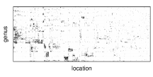
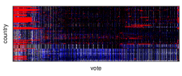
Figure 5: Datasets. Black entries correspond to vfn=1subscript𝑣𝑓𝑛1v_{fn}=1 and white entries correspond to zero values. In the unvote dataset, blue entries represent “abstention” values and red entries are missing votes. For best visualization, rows and columns are re-ordered with complete linkage clustering, except for 1) parliament in which parliament members are sorted by parliamentary group and 2) unvotes where votes are sorted chronologically.

We consider five different public datasets, described next and displayed in Fig. 5.

Animals (animals). The animals dataset (Kemp et al., 2006) contains 50 animals and 85 binary attributes such as nocturnal, hibernates, small or fast. The matrix takes vfn=1subscript𝑣𝑓𝑛1v_{fn}=1 if animal n𝑛n has attribute f𝑓f.

Last.fm (lastfm). We use a binarized subset of the Last.fm dataset (Celma, 2010) where rows correspond to users and columns correspond to musical artists. The matrix takes vfn=1subscript𝑣𝑓𝑛1v_{fn}=1 if user n𝑛n has listened to artist f𝑓f at least once. The matrix has F=285𝐹285F=285 rows and N=1226𝑁1226N=1226 columns.

Paleontological data (paleo). The NOW (New and Old Worlds) fossil mammal database contains information of fossils found in specific paleontological sites (NOW, 2018). From the original paleontological data, we build a matrix where each row is a genus, each column is a location, and vfn=1subscript𝑣𝑓𝑛1v_{fn}=1 if genus f𝑓f has been found at location n𝑛n. We used the same pre-processing as in Bingham et al. (2009) (i.e., we discarded small and infrequent genus, locations with only one genus and kept locations with longitude between 0 and 60 degrees East) and obtained a matrix with F=253𝐹253F=253 rows and N=902𝑁902N=902 columns.

Catalan parliament (parliament). We created a list of the current members of the Catalan parliament and collected the information of who follows whom on Twitter (March 2018). With this data, we created a square adjacency matrix where vfn=1subscript𝑣𝑓𝑛1v_{fn}=1 if member f𝑓f follows member n𝑛n. There are seven political groups represented. The resulting matrix has 135 rows and columns (F=N𝐹𝑁F=N).

UN votes (unvotes). The United Nations General Assembly Voting Data is a dataset that contains the roll-call votes in the UN General Assembly between 1946-2017 (Voeten, 2013). Votes can be yes, no, or abstention. From this data, we created a matrix where vfn=1subscript𝑣𝑓𝑛1v_{fn}=1 if country f𝑓f voted yes to the call n𝑛n, vfn=0subscript𝑣𝑓𝑛0v_{fn}=0 if it voted no, and a missing value if the country did not participate in that call or was not a member of the UN at that time. Next, abstention votes will be treated as either negative votes (no) or missing data, as specified in each experiment. The resulting matrix has F=200𝐹200F=200 rows and N=5429𝑁5429N=5429 columns.

6.2 Methods and setting

State-of-the-art methods. We compare our proposed methods with the following state-of-the-art methods for binary data.

logPCA-K. Probabilistic PCA with Bernoulli likelihood. We use the algorithm presented in Collins et al. (2002). The notation logPCA-K will embed the chosen number of components K𝐾K (e.g., logPCA-8 signifies K=8𝐾8K=8). We used the R package logisticPCA (Landgraf and Lee, 2015) with default parameters.

bICA-K. The binary ICA method introduced in Kabán and Bingham (2008), which uses uncollapsed mean-field variational inference over the partially augmented model (Eqs. (15)-(18)). This is also a parametric method that requires setting K𝐾K.

Proposed methods. Our proposed methods are as follows.

Beta-Dir GS. Estimation in the Beta-Dir model with collapsed Gibbs sampling. Beta parameters are set to αk=βk=1subscript𝛼𝑘subscript𝛽𝑘1\alpha_{k}=\beta_{k}=1. To emulate a nonparametric setting, the Dirichlet parameters are set to γk=1/Ksubscript𝛾𝑘1𝐾\gamma_{k}=1/K and the number of components is set to K=100𝐾100K=100.

Beta-Dir VB. Estimation in the Beta-Dir model with collapsed variational Bayes (CVB0). Beta parameters are set to αk=βk=1subscript𝛼𝑘subscript𝛽𝑘1\alpha_{k}=\beta_{k}=1. To emulate a nonparametric setting, we set γk=1/Ksubscript𝛾𝑘1𝐾\gamma_{k}=1/K and K=100𝐾100K=100.

Dir-Dir GS. Estimation in the Dir-Dir model with collapsed Gibbs sampling. To emulate a nonparametric setting, we set γk=1/Ksubscript𝛾𝑘1𝐾\gamma_{k}=1/K, ηk=1subscript𝜂𝑘1\eta_{k}=1, and K=100𝐾100K=100.

c-bICA-K. Collapsed bICA. The algorithm corresponds to Beta-Dir VB with αk=βk=γk=1subscript𝛼𝑘subscript𝛽𝑘subscript𝛾𝑘1\alpha_{k}=\beta_{k}=\gamma_{k}=1. It is the collapsed version of bICA-K using CVB0 and without the nonparametric approximation.

Implementation details. For each dataset, we ran some preliminary experiments to assess the number of iterations needed by the algorithms to converge. For the Gibbs samplers, we set a conservative burn-in phase of 4,00040004{,}000 iterations and kept the last 1,00010001{,}000 samples of 𝐙𝐙\boldsymbol{\mathbf{Z}} after burn-in. A total number of 500500500 iterations where used for the variational algorithms. In every experiment, we initialized the Gibbs samplers with a random tensor 𝐙𝐙\boldsymbol{\mathbf{Z}} such that 𝐳fn=𝐞ksubscript𝐳𝑓𝑛subscript𝐞𝑘\boldsymbol{\mathbf{z}}_{fn}={\mathbf{e}}_{k} with random k𝑘k. We did not find a special sensitivity to the initial state of the Gibbs Sampler, but we chose a random initialization as a good practice. We also tried initializing with some variational steps, which is another common practice, but did not see significant improvements. Similarly, we initialized the variational algorithms with a random 𝔼[𝐙]𝔼delimited-[]𝐙\mathbb{E}[\boldsymbol{\mathbf{Z}}] such that 𝔼[𝐳fn]=𝐞k𝔼delimited-[]subscript𝐳𝑓𝑛subscript𝐞𝑘\mathbb{E}[\boldsymbol{\mathbf{z}}_{fn}]={\mathbf{e}}_{k} with random k𝑘k. Our variational algorithms are sensitive to the initial state when some components are empty. Because an empty component has a lower probability of being chosen, in practice the variational algorithms are not capable of refilling it again. Initializing from a random state with lots of used components is, therefore, a safer way to avoid these local maxima.

Estimators. The algorithms Beta-Dir GS and Dir-Dir GS return samples from the posterior of p(𝐖,𝐇|𝐕)𝑝𝐖conditional𝐇𝐕p(\boldsymbol{\mathbf{W}},\boldsymbol{\mathbf{H}}|{\mathbf{V}}). Point estimates of the dictionary 𝐖𝐖\boldsymbol{\mathbf{W}} and data expectation 𝐕^=𝐖𝐇^𝐕𝐖𝐇\hat{{\mathbf{V}}}=\boldsymbol{\mathbf{W}}\boldsymbol{\mathbf{H}} are computed by averaging (posterior mean) and by Eq. (33), respectively. Beta-Dir VB, bICA and c-bICA return variational approximations of the posterior of 𝐖𝐖\boldsymbol{\mathbf{W}} and 𝐇𝐇\boldsymbol{\mathbf{H}}. Point estimates of 𝐖𝐖\boldsymbol{\mathbf{W}} and 𝐕^^𝐕\hat{{\mathbf{V}}} are computed from the variational distribution mean and by Eq. (39). logPCA returns maximum likelihood (ML) estimates 𝐖^^𝐖\hat{\boldsymbol{\mathbf{W}}} and 𝐇^^𝐇\hat{\boldsymbol{\mathbf{H}}}. The data expectation is computed as 𝐕^=σ(𝐖^𝐇^)^𝐕𝜎^𝐖^𝐇\hat{{\mathbf{V}}}=\sigma(\hat{{\mathbf{W}}}\hat{{\mathbf{H}}}).

Sensitivity to hyperparameters. When using Dirichlet priors, inferences may be quite sensitive especially for small values of its concentration parameter (Steck and Jaakkola, 2003). For the setting described in Section 6.4, we have tested our algorithms under toy data generated from the model, setting the concentration parameter to 1. We have repeated different inferences with the concentration parameter of the estimator ranging from 0.1 to 10 and observed very small variations on the perplexity (around 0.1, and decreasing as the size of the observed data increases). Thus, for the sake of simplicity, we have therefore decided to set the concentrations parameters to 1 which corresponds to a uniform Dirichlet prior.

Computational cost. The time complexity of the collapsed algorithms is 𝒪(FKN)𝒪𝐹𝐾𝑁\mathcal{O}(FKN) (assuming, for the sake of simplicity, that the Multinomial random number generator is 𝒪(1)𝒪1\mathcal{O}(1)). Note that, unlike some non-mean-parameterized Bernoulli models (Zhou, 2015), or all Poisson models, zeros cannot be ignored because they represent another category, not a lack of observation or a zero-count.

6.3 Dictionary learning and data approximation

6.3.1 Experiments with the parliament dataset

First, we want to form an idea of how well the different models can fit original data. We focus on the parliament dataset, which has reasonable size and a clear structure. We applied the three proposed nonparametric methods Beta-Dir GS, Beta-Dir VB, Dir-Dir GS and the state-of-the-art methods bICA and logPCA. For each method, we compute the negative log-likelihood of the data approximation 𝐕^^𝐕\hat{{\mathbf{V}}}, which serves as a measure of fit:

D(𝐕|𝐕^)=fnlogp(vfn|v^fn).𝐷conditional𝐕^𝐕subscript𝑓𝑛𝑝conditionalsubscript𝑣𝑓𝑛subscript^𝑣𝑓𝑛\displaystyle D({\mathbf{V}}|\hat{{\mathbf{V}}})=-\sum_{fn}\log p(v_{fn}|\hat{v}_{fn}). (66)

bICA was run with increasing values of K𝐾K and the fit ceased increasing for K=8𝐾8K=8 which is the value used in the results (note that in this case 𝐕^^𝐕\hat{{\mathbf{V}}} is the posterior mean estimate and not the ML estimate, so the likelihood is not meant to increase monotonically). logPCA was run with the same value K=8𝐾8K=8. The data approximations 𝐕^^𝐕\hat{{\mathbf{V}}} and dictionaries obtained with the different methods are displayed in Figs. 6 and 7, respectively.

In terms of data approximation, Beta-Dir VB achieves the best fit among the mean-parameterized models in terms of negative log-likelihood (4,72947294{,}729) followed by Beta-Dir GS (4,86348634{,}863). The dictionaries returned by these two algorithms are very similar, with only nine active components. bICA-8 comes next in terms of fit (4,95749574{,}957). We also applied bICA with K>8𝐾8K>8 components but this did not substantially improve the likelihood. Dir-Dir GS returns the worst fit (8,93089308{,}930), with only two active components. Overall logPCA-8 returns the smallest negative log-likelihood (1,78317831{,}783). This due to its larger flexibility as compared to the mean-parameterized models (real-valued factors 𝐖𝐖\boldsymbol{\mathbf{W}} and 𝐇𝐇\boldsymbol{\mathbf{H}}, with product 𝐖𝐇𝐖𝐇\boldsymbol{\mathbf{W}}\boldsymbol{\mathbf{H}} mapped to [0,1]01[0,1]). However, this is at the cost of meaningfulness of the decomposition, as shown in Fig. 7 and explained next.
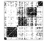
Refer to caption
(a) Original
Refer to caption
(b) Beta-Dir GS
Refer to caption
(c) Beta-Dir VB
Refer to caption
(d) Dir-Dir GS
Refer to caption
(e) bICA-8
Refer to caption
(f) logPCA-8
Figure 6: Reconstructed matrices for the parliament dataset.

In dictionary learning, we want to learn a meaningful decomposition of the data. The columns of the dictionary 𝐖𝐖\boldsymbol{\mathbf{W}} are expected to contain patterns or prototypes characteristic of the data. In particular, NMF is known to produce so-called part-based representations (each sample, a column of 𝐕𝐕\boldsymbol{\mathbf{V}}, is approximated as a constructive linear combination of building units) (Lee and Seung, 1999). When the rows of the dictionary are given Dirichlet priors, 𝐰fsubscript𝐰𝑓{\mathbf{w}}_{f} can also be interpreted as the probability distribution of feature f𝑓f over the K𝐾K components. In Fig. 7, the rows of the dictionaries displayed correspond to members of the parliament (MP). For each MP we show its Twitter username and its political party. The dictionaries returned by the mean-parameterized factorization methods are easily interpretable. In particular, the dictionaries returned by Beta-Dir GS, Beta-Dir VB and to some extent bICA-8 closely reflect the party memberships of the MPs. Dir-Dir GS, which is based on a less flexible model, only captures two sets of MPs, one with the members of Cs (the main opposition party) and the other with members of the remaining parties, regardless of political alignment (left-wing, right-wing, independentist and anti-independentist). In contrast, the dictionary returned by logPCA-8 is much more difficult to interpret.
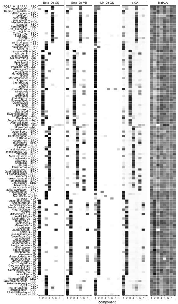
Refer to caption
Figure 7: Estimated dictionaries from the parliament dataset. Members are sorted by party and then alphabetically. Columns are sorted by their norm. Only the first eight columns are displayed for the nonparametric methods Beta-Dir GS, Beta-Dir VB and Dir-Dir GS. The results displayed for bICA and logPCA are with K=8𝐾8K=8. The values of 𝐖𝐖\boldsymbol{\mathbf{W}} estimated by logPCA-8 belong to the [207.17,217.92]207.17217.92[-207.17,217.92] range and have been linearly mapped to the [0,1]01[0,1] range for visual display.

6.3.2 Experiments with the unvotes dataset

In this section, we consider a subset of unvotes, reduced to the 1946-1990 range which corresponds to the Cold War period. Furthermore, the abstentions are here treated as missing values. Fig. 8 shows the dictionaries learned by the five considered methods. As before, bICA was applied with various values of K𝐾K and we selected the value that leads to the smallest negative log-likelihood (K=7𝐾7K=7). Accordingly, logPCA was also applied with K=7𝐾7K=7.

Fig. 8 shows that Beta-Dir GS returns the finest dictionary, detecting political blocks that tended to vote similarly in the UN assembly and capturing some nuances that the other algorithms do not find. European countries (and members or allies of NATO such as the USA, Japan, or Australia) are concentrated in one component, denoting similar voting strategies. The former members of the Soviet Union and the Warsaw Pact also form a block of their own, with some allies such as Cuba or the former Yugoslavia. Members of the Non-Aligned Movement (even countries that became members after 1991, such as Guatemala, Thailand, or Haiti), from Egypt to Cuba and from Honduras to Haiti, are split into two blocks: the Latin American group and the Asian-African group. Another detected alliance is between the United States and Israel, which are distributed between the European component and a component of their own. Beta-Dir VB detects the split between the Warsaw and NATO blocks, and the alliance between the USA and Israel, but it fails to detect the two subgroups of the Non-Aligned Movement, which is considered a single block. bICA-7 returns similar results to Beta-Dir GS but fails to detect the alliance between the USA and Israel. Note that the results of bICA are obtained with a well-chosen value of K𝐾K while Beta-Dir GS automatically detects a suitable value. The underlying assumption of Dir-Dir (one topic per country and one topic per vote) seems too simplistic for this dataset, and the algorithm puts every country in the same component. Again and as somewhat expected, the dictionary learned by logPCA is more difficult to interpret.
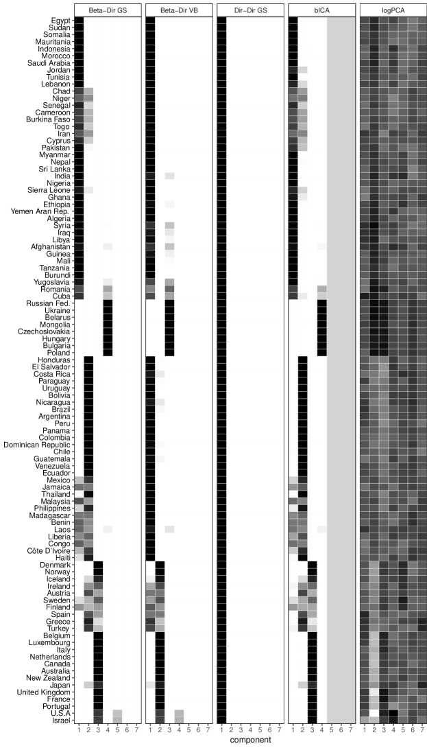
Refer to caption
Figure 8: Estimated dictionaries from the unvotes dataset. Columns are sorted by their norm. Only the first seven columns are displayed for the nonparametric methods Beta-Dir GS, Beta-Dir VB and Dir-Dir GS. The results displayed for bICA and logPCA are with K=4𝐾4K=4 and K=7𝐾7K=7, respectively. The values of 𝐖𝐖\boldsymbol{\mathbf{W}} estimated by logPCA-7 belong to the [629.7,335.1]629.7335.1[-629.7,335.1] range and have been linearly mapped to the [0,1]01[0,1] range for visual display.

6.3.3 Experiments with the paleo dataset

We finally look into the dictionaries returned by the five considered method on the paleo dataset, see Fig. 9. The same strategy was applied to find a suitable value of K𝐾K for bICA and logPCA, leading to K=7𝐾7K=7. The results can be read as the probability of a genus to be found in a set of prototypical locations. Interestingly, Dir-Dir GS is the method that returns the most detailed dictionary for this dataset. The other methods tend to produce larger clusters of genera. This highlights the importance of choosing the right model for each dataset since they imply different underlying assumptions. Dir-Dir GS assumes one topic per genus and one topic per location. We will see in the following section that Dir-Dir GS also gives the best predictions for this dataset. Again, the dictionary obtained with logPCA is harder to interpret.
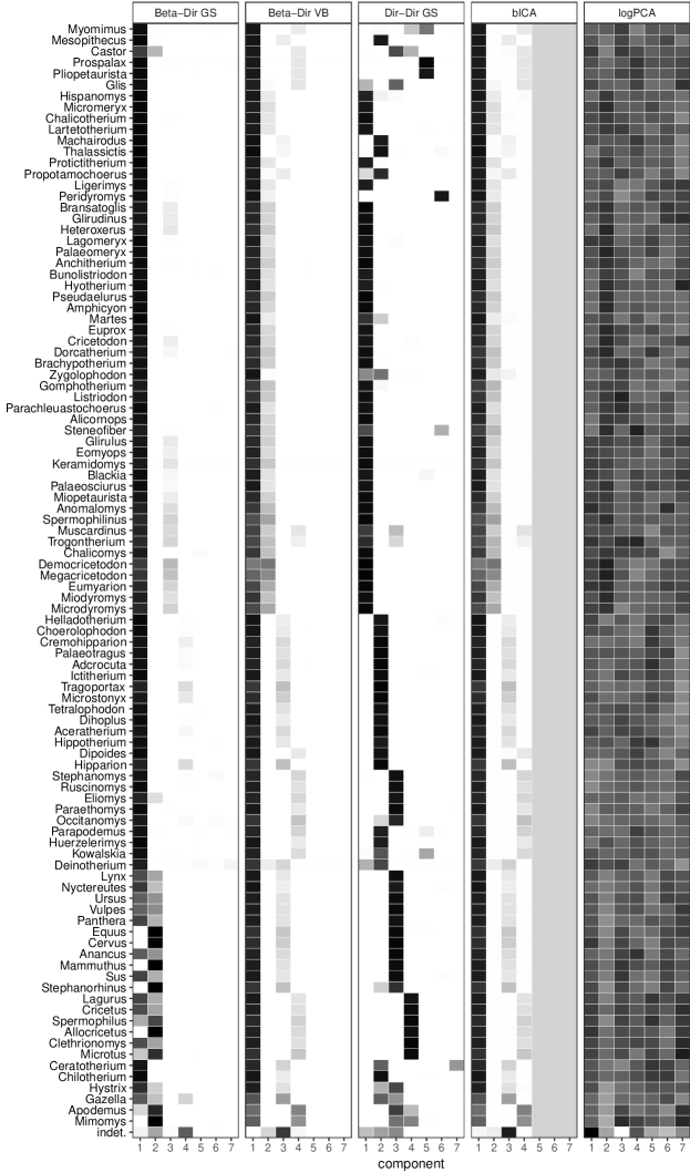
Refer to caption
Figure 9: Estimated dictionaries from the paleo dataset. Columns are sorted by their norm. Only the first seven columns are displayed for the nonparametric methods Beta-Dir GS, Beta-Dir VB and Dir-Dir GS. The results displayed for bICA and logPCA are with K=4𝐾4K=4 and K=7𝐾7K=7, respectively. The values of 𝐖𝐖\boldsymbol{\mathbf{W}} estimated by logPCA-7 belong to the [102.3,118.7]102.3118.7[-102.3,118.7] range and have been linearly mapped to the [0,1]01[0,1] range for visual display.

6.4 Prediction

6.4.1 Experimental setting

We now evaluate the capability of the five previously considered methods together with c-bICA to predict missing data. For each of the five considered datasets, we applied the algorithms to a 75%percent7575\% random subset of the original data. We here use the full unvotes in which abstentions are treated as negative votes (vfn=0subscript𝑣𝑓𝑛0v_{fn}=0). bICA and c-bICA where applied with K=2,,8𝐾28K=2,\ldots,8. logPCA was applied with K=2,,4𝐾24K=2,\ldots,4. Then we computed the perplexity of the test set (the 25% held-out entries) given the estimate 𝐕^=𝐄[𝐖𝐇|𝐕train]^𝐕𝐄delimited-[]conditional𝐖𝐇subscript𝐕train\hat{\boldsymbol{\mathbf{V}}}=\mathbf{E}[\boldsymbol{\mathbf{WH}}|\boldsymbol{\mathbf{V}}_{\text{train}}] (for all methods except logPCA-K) or 𝐕^=σ(𝐖^𝐇^)^𝐕𝜎^𝐖^𝐇\hat{\boldsymbol{\mathbf{V}}}=\sigma(\hat{\boldsymbol{\mathbf{W}}}\hat{\boldsymbol{\mathbf{H}}}) (for logPCA). The perplexity is here simply taken as the negative log-likelihood of the test set (Hofmann, 1999):

perplexity=1T(f,n)testlogp(vfn|𝐕^)𝑝𝑒𝑟𝑝𝑙𝑒𝑥𝑖𝑡𝑦1𝑇subscript𝑓𝑛test𝑝conditionalsubscript𝑣𝑓𝑛^𝐕\displaystyle perplexity=-\frac{1}{T}\sum_{(f,n)\in\text{test}}\log p(v_{fn}|\hat{\boldsymbol{\mathbf{V}}}) (67)

where T𝑇T is the number of elements in the test set (in our case, T=0.25FN𝑇0.25𝐹𝑁T=0.25FN).

6.4.2 Prediction performance

Fig. 10 displays the perplexities obtained by all methods from 10 repetitions of the experiment with randomly selected training and test sets, and random initializations (the same starting point is used for bICA and c-bICA). The proposed Beta-Dir VB performs similarly or better (lastfm, parliament) than bICA, while automatically adjusting the number of relevant components. As hinted from the dictionary learning experiments, Dir-Dir GS performs considerably better than the other mean-parameterized methods on the paleo dataset. c-bICA does not specifically improve over bICA (remember they are based on the same model, only inference changes) and performs worse in some cases (lastfm, parliament). However, its performance is more stable, with less variation between different runs, a likely consequence of the collapsed inference.

Despite its flexibility (unconstrained 𝐖𝐖\boldsymbol{\mathbf{W}} and 𝐇𝐇\boldsymbol{\mathbf{H}}), logPCA provides marginally better perplexity (except on the animal dataset where it performs worse than almost all other methods), and only given a suitable value of K𝐾K. Its predictive performance can drastically decay with ill-chosen values of K𝐾K. In contrast, our proposed methods do not require tuning K𝐾K to a proper value. Furthermore, they provide competitive prediction performance together with the interpretability of the decomposition. We have also compared against a standard LDA using the same range of K𝐾K than logPCA, but the perplexity was much worse (around six) for all datasets; we did not plot it due to the high difference in the scale.
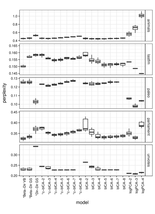
Refer to caption
Figure 10: Prediction performance measured by perplexity (lower values are better). The methods introduced in this paper are marked with an asterisk.

6.4.3 Convergence of the variational inference algorithms

Fig. 11 displays the average perplexity values returned by the variational algorithms Beta-Dir VB, c-bICA-5 and bICA-5 along iterations. As expected, c-bICA tends to converge faster than bICA though not consistently so. Being initialized with a full tensor of dimension K=100𝐾100K=100 (as described in Section 6.2), Beta-Dir VB starts with a relatively higher perplexity but catches up with the two other methods in a reasonable number of iterations.
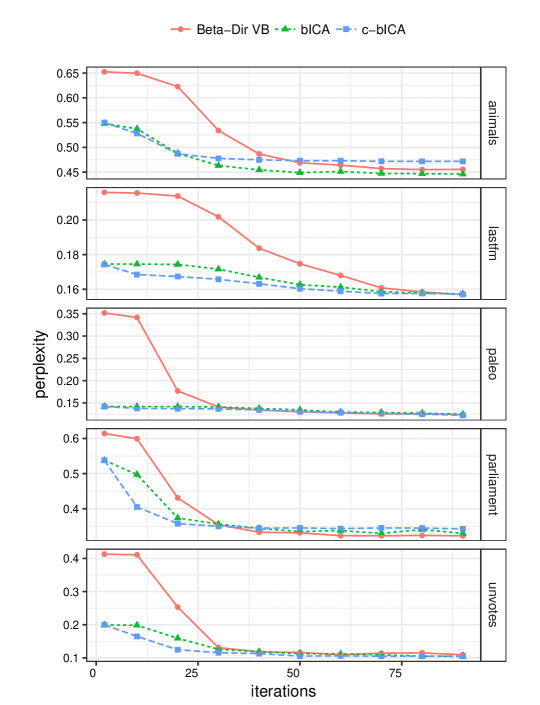
Refer to caption
Figure 11: Average perplexity (over 10 repetitions) returned by the variational inference algorithms along iterations.

7 Conclusions

We have presented a unified view for Bayesian mean-parameterized NBMF. The interest of mean-parameterized models in NMF is that they keep factors interpretable since they belong to the same space than the observed data. We have addressed three models that correspond to three possible sets of constraints that each respect mean-parameterization. One model, Dir-Beta, is a Bayesian extension of the Aspect Bernoulli model of Bingham et al. (2009). Another model, Beta-Dir, corresponds to the binary ICA model of Kabán and Bingham (2008). We have proposed a new collapsed Gibbs sampler and a new collapsed variational inference method for estimation in these models. We have proposed a novel, third model, Dir-Dir, and we have designed a collapsed Gibbs sampler for inference with this model. Lastly, we have proposed a nonparametric extension for these three models. Experiments have shown that our nonparametric methods can achieve similar performance than the state-of-the-art methods applied with a suitable value of K𝐾K. As expected, the more flexible logPCA can achieve better data approximation and in some cases prediction, but at the cost of interpretation which of utter importance in some applications.

Acknowledgements

This work has received funding from the European Research Council (ERC) under the European Union’s Horizon 2020 research and innovation programme under grant agreement No 681839 (project FACTORY).

References

  • Aldous (1985) Aldous DJ (1985) Exchangeability and related topics. In: École d’été de probabilités de Saint-Flour, XIII—1983, Lecture Notes in Mathematics, vol 1117, Springer, Berlin, pp 1–198
  • Alquier and Guedj (2017) Alquier P, Guedj B (2017) An oracle inequality for quasi-bayesian nonnegative matrix factorization. Mathematical Methods of Statistics 26(1):55–67
  • Anderson (1991) Anderson JR (1991) The adaptive nature of human categorization. Psychological Review 98:409–429
  • Asuncion et al. (2009) Asuncion A, Welling M, Smyth P, Teh YW (2009) On smoothing and inference for topic models. In: Proceedings of the 25th Conference on Uncertainty in Artificial Intelligence (UAI ’09), pp 27–34
  • Bingham et al. (2009) Bingham E, Kabán A, Fortelius M (2009) The Aspect Bernoulli model: Multiple causes of presences and absences. Pattern Analysis and Applications 12(1):55–78
  • Blei et al. (2003) Blei DM, Ng AY, Jordan MI (2003) Latent Dirichlet allocation. Journal of Machine Learning Research 3(Jan):993–1022
  • Buntine and Jakulin (2006) Buntine WL, Jakulin A (2006) Discrete component analysis. In: Lecture Notes in Computer Science, Springer, vol 3940, pp 1–33
  • Canny (2004) Canny J (2004) GaP: A factor model for discrete data. In: Proceedings of the 27th Annual International ACM SIGIR Conference on Research and Development in Information Retrieval (SIGIR ’04), pp 122–129
  • Çapan et al. (2018) Çapan G, Akbayrak S, Ceritli TY, Cemgil AT (2018) Sum conditioned Poisson factorization. In: Proceedings of the 14th International Conference on Latent Variable Analysis and Signal Separation (LVA/ICA ’18), pp 24–35
  • Celma (2010) Celma O (2010) Music recommendation and discovery in the long tail. Springer
  • Cemgil (2009) Cemgil AT (2009) Bayesian inference for nonnegative matrix factorisation models. Computational Intelligence and Neuroscience 2009:1–17
  • Cichocki et al. (2008) Cichocki A, Lee H, Kim YD, Choi S (2008) Non-negative matrix factorization with α𝛼\alpha-divergence. Pattern Recognition Letters 29(9):1433–1440
  • Collins et al. (2002) Collins M, Dasgupta S, Schapire RE (2002) A generalization of principal components analysis to the exponential family. In: Advances in Neural Information Processing Systems 14, MIT Press, pp 617–624
  • Févotte and Idier (2011) Févotte C, Idier J (2011) Algorithms for nonnegative matrix factorization with the β𝛽\beta-divergence. Neural Computation 23(9):2421–2456
  • Gopalan et al. (2014) Gopalan P, Ruiz FJR, Ranganath R, Blei DM (2014) Bayesian nonparametric Poisson factorization for recommendation systems. Journal of Machine Learning Research 33:275–283
  • Gopalan et al. (2015) Gopalan P, Hofman JM, Blei DM (2015) Scalable recommendation with hierarchical Poisson factorization. In: Proceedings of the 31st Conference on Uncertainty in Artificial Intelligence (UAI ’15), pp 326–335
  • He et al. (2017) He X, Liao L, Zhang H, Nie L, Hu X, Chua TS (2017) Neural collaborative filtering. In: Proceedings of the 26th International Conference on World Wide Web (WWW ’17), International World Wide Web Conferences Steering Committee, p 173–182
  • Hernandez-Lobato et al. (2014) Hernandez-Lobato JM, Houlsby N, Ghahramani Z (2014) Stochastic inference for scalable probabilistic modeling of binary matrices. Proceedings of the 31st International Conference on Machine Learning (ICML ’14) 32:1–6
  • Hoffman et al. (2010) Hoffman MD, Blei DM, Cook PR (2010) Bayesian nonparametric matrix factorization for recorded music. In: Proceedings of the 27th International Conference on International Conference on Machine Learning (ICML ’10), pp 439–446
  • Hoffman et al. (2013) Hoffman MD, Blei DM, Wang C, Paisley J (2013) Stochastic variational inference. Journal of Machine Learning Research 14(1):1303–1347
  • Hofmann (1999) Hofmann T (1999) Probabilistic latent semantic analysis. In: Proceedings of the 15th Conference on Uncertainty in Artificial Intelligence (UAI ’99), pp 289–296
  • Ishiguro et al. (2017) Ishiguro K, Sato I, Ueda N (2017) Averaged collapsed variational Bayes inference. Journal of Machine Learning Research 18(1):1–29
  • Kabán and Bingham (2008) Kabán A, Bingham E (2008) Factorisation and denoising of 0-1 data: A variational approach. Neurocomputing 71(10-12):2291–2308
  • Kemp et al. (2006) Kemp C, Tenenbaum JB, Griffiths TL, Yamada T, Ueda N (2006) Learning systems of concepts with an infinite relational model. In: Proceedings of the 21st National Conference on Artificial Intelligence (AAAI ’06), pp 381–388
  • Landgraf and Lee (2015) Landgraf AJ, Lee Y (2015) Dimensionality reduction for binary data through the projection of natural parameters. Tech. Rep. 890, Department of Statistics, The Ohio State University
  • Larsen and Clemmensen (2015) Larsen JS, Clemmensen LKH (2015) Non-negative matrix factorization for binary data. In: Proceedings of the 7th International Joint Conference on Knowledge Discovery, Knowledge Engineering and Knowledge Management (IC3K ’15), pp 555–563
  • Lee and Seung (1999) Lee DD, Seung HS (1999) Learning the parts of objects with nonnegative matrix factorization. Nature 401:788–791
  • Lee and Seung (2001) Lee DD, Seung HS (2001) Algorithms for non-negative matrix factorization. In: Advances in Neural Information Processing Systems 13, pp 556–562
  • Liu (1994) Liu JS (1994) The collapsed Gibbs sampler in Bayesian computations with applications to a gene regulation problem. Journal of the American Statistical Association 89(427):958–966
  • Meeds et al. (2007) Meeds E, Ghahramani Z, Neal RM, Roweis ST (2007) Modeling dyadic data with binary latent factors. In: Advances in Neural Information Processing Systems 19, MIT Press, pp 977–984
  • Miettinen et al. (2008) Miettinen P, Mielikäinen T, Gionis A, Das G, Mannila H (2008) The discrete basis problem. IEEE Transactions on Knowledge and Data Engineering 20(10):1348–1362
  • NOW (2018) NOW (2018) The NOW community. new and old worlds database of fossil mammals (NOW). URL http://www.helsinki.fi/science/now/, release 030717, retrieved May 2018
  • Pitman (2002) Pitman J (2002) Combinatorial stochastic processes. Lecture Notes in Mathematics, Springer-Verlag, Berlin, lectures from the 32nd Summer School on Probability Theory held in Saint-Flour
  • Polson et al. (2013) Polson NG, Scott JG, Windle J (2013) Bayesian inference for logistic models using Polya-Gamma latent variables. Journal of the American Statistical Association 108:1339–1349
  • R Core Team (2017) R Core Team (2017) R: A language and environment for statistical computing. R Foundation for Statistical Computing, URL https://www.R-project.org/
  • Rukat et al. (2017) Rukat T, Holmes CC, Titsias MK, Yau C (2017) Bayesian Boolean matrix factorisation. In: Proceedings of the 34th International Conference on Machine Learning (ICML ’17), pp 2969–2978
  • Sammel et al. (1997) Sammel MD, Ryan LM, Legler JM (1997) Latent variable models for mixed discrete and continuous outcomes. Journal of the Royal Statistical Society Series B (Methodological) 59(3):667–678
  • Schein et al. (2003) Schein AI, Saul LK, Ungar LH (2003) A generalized linear model for principal component analysis of binary data. In: Proceedings of the 9th Workshop on Artificial Intelligence and Statistics (AISTATS ’03), pp 14–21
  • Schmidt et al. (2009) Schmidt MN, Winther O, Hansen LK (2009) Bayesian non-negative matrix factorization. In: Proceedings of the 8th International Conference on Independent Component Analysis and Signal Separation (ICA ’09), pp 540–547
  • Singh and Gordon (2008) Singh AP, Gordon GJ (2008) A unified view of matrix factorization models. In: Proceedings of the European Conference on Machine Learning and Knowledge Discovery in Databases (ECML-PKDD ’08), pp 358–373
  • Slawski et al. (2013) Slawski M, Hein M, Lutsik P (2013) Matrix factorization with binary components. In: Advances in Neural Information Processing Systems 26, Curran Associates, Inc., pp 3210–3218
  • Sørensen (1948) Sørensen T (1948) A method of establishing groups of equal amplitude in plant sociology based on similarity of species and its application to analyses of the vegetation on Danish commons. Biologiske Skrifter 5:1–34
  • Steck and Jaakkola (2003) Steck H, Jaakkola TS (2003) On the Dirichlet prior and Bayesian regularization. In: Advances in Neural Information Processing Systems 15, MIT Press, pp 713–720
  • Teh et al. (2006) Teh YW, Jordan MI, Beal MJ, Blei DM (2006) Hierarchical Dirichlet processes. Journal of the American Statistical Association 101(476):1566–1581
  • Teh et al. (2007) Teh YW, Newman D, Welling M (2007) A collapsed variational Bayesian inference alzgorithm for latent Dirichlet allocation. In: Advances in Neural Information Processing Systems 19, MIT Press, pp 1353–1360
  • Tipping (1999) Tipping ME (1999) Probabilistic visualisation of high-dimensional binary data. In: Advances in Neural Information Processing Systems 11, MIT Press, pp 592–598
  • Tipping and Bishop (1999) Tipping ME, Bishop C (1999) Probabilistic principal component analysis. Journal of the Royal Statistical Society, Series B 21/3:611–622
  • Tomé et al. (2013) Tomé AM, Schachtner R, Vigneron V, Puntonet CG, Lang EW (2013) A logistic non-negative matrix factorization approach to binary data sets. Multidimensional Systems and Signal Processing 26(1):125–143
  • Udell et al. (2016) Udell M, Horn C, Zadeh R, Boyd S (2016) Generalized low rank models. Foundations and Trends in Machine Learning 9(1):1–118
  • Voeten (2013) Voeten E (2013) Data and analyses of voting in the UN General Assembly. In: Reinal B (ed) Routledge Handbook of International Organization, Routledge
  • Xue et al. (2017) Xue HJ, Dai XY, Zhang J, Huang S, Chen J (2017) Deep matrix factorization models for recommender systems. In: Proceedings of the 26th International Joint Conference on Artificial Intelligence (IJCAI ’17), AAAI Press, p 3203–3209
  • Zhang et al. (2009) Zhang ZY, Li T, Ding C, Ren XW, Zhang XS (2009) Binary matrix factorization for analyzing gene expression data. Data Mining and Knowledge Discovery 20(1):28–52
  • Zhou (2015) Zhou M (2015) Infinite edge partition models for overlapping community detection and link prediction. In: Proceedings of the 18th International Conference on Artificial Intelligence and Statistics (AISTATS ’15), pp 1135–1143
  • Zhou et al. (2012) Zhou M, Hannah L, Dunson D, Carin L (2012) Beta-negative binomial process and Poisson factor analysis. In: Proceedings of the 15th International Conference on Artificial Intelligence and Statistics (AISTATS ’12), pp 1462–1471
  • Zhou et al. (2016) Zhou M, Cong Y, Chen B (2016) Augmentable Gamma belief networks. Journal of Machine Learning Research 17(163):1–44

Appendix A Probability distributions functions

A.1 Bernoulli distribution

Distribution over a binary variable x{0,1}𝑥01x\in\{0,1\}, with mean parameter μ[0,1]𝜇01\mu\in[0,1]:

Bernoulli(x|μ)Bernoulliconditional𝑥𝜇\displaystyle\text{Bernoulli}(x|\mu) =μx(1μ)1x.absentsuperscript𝜇𝑥superscript1𝜇1𝑥\displaystyle=\mu^{x}(1-\mu)^{1-x}. (68)

A.2 Beta distribution

Distribution over a continuous variable x[0,1]𝑥01x\in[0,1], with shape parameters a>0𝑎0a>0, b>0𝑏0b>0:

Beta(x|a,b)Betaconditional𝑥𝑎𝑏\displaystyle\text{Beta}(x|a,b) =Γ(a+b)Γ(a)Γ(b)xa1(1x)b1.absentΓ𝑎𝑏Γ𝑎Γ𝑏superscript𝑥𝑎1superscript1𝑥𝑏1\displaystyle=\frac{\Gamma(a+b)}{\Gamma(a)\Gamma(b)}x^{a-1}(1-x)^{b-1}. (69)

A.3 Gamma distribution

Distribution for a continuous variable x>0𝑥0x>0, with shape parameter a>0𝑎0a>0 and rate parameter b>0𝑏0b>0:

Gamma(x|a,b)Gammaconditional𝑥𝑎𝑏\displaystyle\text{Gamma}(x|a,b) =baΓ(a)xa1ebx.absentsuperscript𝑏𝑎Γ𝑎superscript𝑥𝑎1superscript𝑒𝑏𝑥\displaystyle=\frac{b^{a}}{\Gamma(a)}x^{a-1}e^{-bx}. (70)

A.4 Dirichlet distribution

Distribution for K𝐾K continuous variables xk[0,1]subscript𝑥𝑘01x_{k}\in[0,1] such that kxk=1subscript𝑘subscript𝑥𝑘1\sum_{k}x_{k}=1. Governed by K𝐾K shape parameters α1,αKsubscript𝛼1subscript𝛼𝐾\alpha_{1},...\alpha_{K} such that αk>0subscript𝛼𝑘0\alpha_{k}>0:

Dirichlet(𝐱|𝜶)Dirichletconditional𝐱𝜶\displaystyle\text{Dirichlet}(\boldsymbol{\mathbf{x}}|\boldsymbol{\mathbf{\alpha}}) =Γ(kαk)kΓ(αk)kxαk1.absentΓsubscript𝑘subscript𝛼𝑘subscriptproduct𝑘Γsubscript𝛼𝑘subscriptproduct𝑘superscript𝑥subscript𝛼𝑘1\displaystyle=\frac{\Gamma(\sum_{k}\alpha_{k})}{\prod_{k}\Gamma(\alpha_{k})}\prod_{k}x^{\alpha_{k}-1}. (71)

A.5 Discrete distribution

Distribution for the discrete variable 𝐱{𝐞1,,𝐞K}𝐱subscript𝐞1subscript𝐞𝐾{\mathbf{x}}\in\{{\mathbf{e}}_{1},\ldots,{\mathbf{e}}_{K}\}, where 𝐞isubscript𝐞𝑖{\mathbf{e}}_{i} is the ithsuperscript𝑖𝑡i^{th} canonical vector. Governed by the discrete probabilities μ1,,μKsubscript𝜇1subscript𝜇𝐾\mu_{1},...,\mu_{K} such that μk[0,1]subscript𝜇𝑘01\mu_{k}\in[0,1] and kμk=1subscript𝑘subscript𝜇𝑘1\sum_{k}\mu_{k}=1:

p(𝐱=𝐞k)=μk𝑝𝐱subscript𝐞𝑘subscript𝜇𝑘\displaystyle p({\mathbf{x}}={\mathbf{e}}_{k})=\mu_{k} (72)

The probability mass function can be written as:

Discrete(𝐱|𝝁)Discreteconditional𝐱𝝁\displaystyle\text{Discrete}(\boldsymbol{\mathbf{x}}|\boldsymbol{\mathbf{\mu}}) =kμkxk.absentsubscriptproduct𝑘superscriptsubscript𝜇𝑘subscript𝑥𝑘\displaystyle=\prod_{k}\mu_{k}^{x_{k}}. (73)

We may write Discrete(𝐱|𝝁)=Multinomial(𝐱|1,𝝁)Discreteconditional𝐱𝝁Multinomialconditional𝐱1𝝁\text{Discrete}(\boldsymbol{\mathbf{x}}|\boldsymbol{\mathbf{\mu}})=\text{Multinomial}(\boldsymbol{\mathbf{x}}|1,\boldsymbol{\mathbf{\mu}}).

A.6 Multinomial distribution

Distribution for an integer-valued vector 𝐱=[x1,,xK]TK𝐱superscriptsubscript𝑥1subscript𝑥𝐾𝑇superscript𝐾\boldsymbol{\mathbf{x}}=[x_{1},...,x_{K}]^{T}\in\mathbb{N}^{K}. Governed by the total number L=kxk𝐿subscript𝑘subscript𝑥𝑘L=\sum_{k}x_{k} of events assigned to K𝐾K bins and the probabilities μksubscript𝜇𝑘\mu_{k} of being assigned to bin k𝑘k:

Multinomial(𝐱|L,𝝁)Multinomialconditional𝐱𝐿𝝁\displaystyle\text{Multinomial}(\boldsymbol{\mathbf{x}}|L,\boldsymbol{\mathbf{\mu}}) =L!x1!xK!kμkxk.absent𝐿𝑥1subscript𝑥𝐾subscriptproduct𝑘superscriptsubscript𝜇𝑘subscript𝑥𝑘\displaystyle=\frac{L!}{x1!...x_{K}!}\prod_{k}\mu_{k}^{x_{k}}. (74)

Appendix B Derivations for the Beta-Dir model

B.1 Marginalizing out 𝐖𝐖\boldsymbol{\mathbf{W}} and 𝐇𝐇\boldsymbol{\mathbf{H}} from the joint likelihood

We seek to compute marginal joint probability introduced in Eq. (22) and given by:

p(𝐕,𝐙)=fp(𝐰f)np(𝐳fn|𝐰f)d𝐰fp(𝐙¯f)nkp(hkn)fp(vfn|𝐡n,𝐳fn)d𝐡np(𝐯n|𝐙n).𝑝𝐕𝐙subscriptproduct𝑓superscript𝑝subscript𝐰𝑓subscriptproduct𝑛𝑝conditionalsubscript𝐳𝑓𝑛subscript𝐰𝑓𝑑subscript𝐰𝑓𝑝subscript¯𝐙𝑓subscriptproduct𝑛superscriptsubscriptproduct𝑘𝑝subscript𝑘𝑛subscriptproduct𝑓𝑝conditionalsubscript𝑣𝑓𝑛subscript𝐡𝑛subscript𝐳𝑓𝑛𝑑subscript𝐡𝑛𝑝conditionalsubscript𝐯𝑛subscript𝐙𝑛\displaystyle p(\mathbf{V},\mathbf{Z})=\prod_{f}\overbrace{\int p(\boldsymbol{\mathbf{w}}_{f})\prod_{n}p(\boldsymbol{\mathbf{z}}_{fn}|\boldsymbol{\mathbf{w}}_{f})\,d\mathbf{w}_{f}}^{p(\underline{\boldsymbol{\mathbf{Z}}}_{f})}\prod_{n}\overbrace{\int\prod_{k}p(h_{kn})\prod_{f}p(v_{fn}|\boldsymbol{\mathbf{h}}_{n},\boldsymbol{\mathbf{z}}_{fn})\,d{\mathbf{h}}_{n}}^{p(\boldsymbol{\mathbf{v}}_{n}|\boldsymbol{\mathbf{Z}}_{n})}.

Using the expression of the normalization constant of the Dirichlet distribution, the first integral can be computed as follows:

p(𝐙¯f)𝑝subscript¯𝐙𝑓\displaystyle p(\underline{\boldsymbol{\mathbf{Z}}}_{f}) =p(𝐰f)np(𝐳fn|𝐰f)d𝐰fabsent𝑝subscript𝐰𝑓subscriptproduct𝑛𝑝conditionalsubscript𝐳𝑓𝑛subscript𝐰𝑓𝑑subscript𝐰𝑓\displaystyle=\int p(\boldsymbol{\mathbf{w}}_{f})\prod_{n}p(\boldsymbol{\mathbf{z}}_{fn}|\boldsymbol{\mathbf{w}}_{f})\,d\mathbf{w}_{f} (75)
=Γ(kγk)kΓ(γk)kwfkγk1nwfkzfknd𝐰fabsentΓsubscript𝑘subscript𝛾𝑘subscriptproduct𝑘Γsubscript𝛾𝑘subscriptproduct𝑘superscriptsubscript𝑤𝑓𝑘subscript𝛾𝑘1subscriptproduct𝑛superscriptsubscript𝑤𝑓𝑘subscript𝑧𝑓𝑘𝑛𝑑subscript𝐰𝑓\displaystyle=\int\frac{\Gamma(\sum_{k}\gamma_{k})}{\prod_{k}\Gamma(\gamma_{k})}\prod_{k}w_{fk}^{\gamma_{k}-1}\prod_{n}w_{fk}^{z_{fkn}}\,d\mathbf{w}_{f} (76)
=Γ(kγk)kΓ(γk)kwfkγk+Lfk1d𝐰fabsentΓsubscript𝑘subscript𝛾𝑘subscriptproduct𝑘Γsubscript𝛾𝑘subscriptproduct𝑘superscriptsubscript𝑤𝑓𝑘subscript𝛾𝑘subscript𝐿𝑓𝑘1𝑑subscript𝐰𝑓\displaystyle=\frac{\Gamma(\sum_{k}\gamma_{k})}{\prod_{k}\Gamma(\gamma_{k})}\int\prod_{k}w_{fk}^{\gamma_{k}+L_{fk}-1}\,d\mathbf{w}_{f} (77)
=Γ(kγk)kΓ(γk)kΓ(γk+Lfk)Γ(kγk+Lfk).absentΓsubscript𝑘subscript𝛾𝑘subscriptproduct𝑘Γsubscript𝛾𝑘subscriptproduct𝑘Γsubscript𝛾𝑘subscript𝐿𝑓𝑘Γsubscript𝑘subscript𝛾𝑘subscript𝐿𝑓𝑘\displaystyle=\frac{\Gamma(\sum_{k}\gamma_{k})}{\prod_{k}\Gamma(\gamma_{k})}\frac{\prod_{k}\Gamma(\gamma_{k}+L_{fk})}{\Gamma(\sum_{k}\gamma_{k}+L_{fk})}. (78)

The second integral in Eq. (22) is computed as follows. In Eq. (80) we use that p(vfn|𝐡n,𝐳fn)=Bernoulli(vfn|khknzfkn)=kBernoulli(vfn|hkn)zfkn𝑝conditionalsubscript𝑣𝑓𝑛subscript𝐡𝑛subscript𝐳𝑓𝑛Bernoulliconditionalsubscript𝑣𝑓𝑛subscriptproduct𝑘superscriptsubscript𝑘𝑛subscript𝑧𝑓𝑘𝑛subscriptproduct𝑘Bernoullisuperscriptconditionalsubscript𝑣𝑓𝑛subscript𝑘𝑛subscript𝑧𝑓𝑘𝑛p(v_{fn}|\boldsymbol{\mathbf{h}}_{n},\boldsymbol{\mathbf{z}}_{fn})=\text{Bernoulli}(v_{fn}|\prod_{k}h_{kn}^{z_{fkn}})=\prod_{k}\text{Bernoulli}(v_{fn}|h_{kn})^{z_{fkn}} (recall that 𝐳fnsubscript𝐳𝑓𝑛\mathbf{z}_{fn} is an indicator vector). In Eq. (83), we use the expression of the normalization constant of the Beta distribution.

p(𝐯n|𝐙n)𝑝conditionalsubscript𝐯𝑛subscript𝐙𝑛\displaystyle p(\boldsymbol{\mathbf{v}}_{n}|\boldsymbol{\mathbf{Z}}_{n}) =kp(hkn)fp(vfn|𝐡n,𝐳fn)d𝐡nabsentsubscriptproduct𝑘𝑝subscript𝑘𝑛subscriptproduct𝑓𝑝conditionalsubscript𝑣𝑓𝑛subscript𝐡𝑛subscript𝐳𝑓𝑛𝑑subscript𝐡𝑛\displaystyle=\int\prod_{k}p(h_{kn})\prod_{f}p(v_{fn}|\boldsymbol{\mathbf{h}}_{n},\boldsymbol{\mathbf{z}}_{fn})\,{d\mathbf{h}_{n}} (79)
=k[Γ(αk+βk)Γ(αk)Γ(βk)hknαk1(1hkn)βk1]fk[hknvfn(1hkn)1vfn]zfknd𝐡nabsentsubscriptproduct𝑘delimited-[]Γsubscript𝛼𝑘subscript𝛽𝑘Γsubscript𝛼𝑘Γsubscript𝛽𝑘superscriptsubscript𝑘𝑛subscript𝛼𝑘1superscript1subscript𝑘𝑛subscript𝛽𝑘1subscriptproduct𝑓𝑘superscriptdelimited-[]superscriptsubscript𝑘𝑛subscript𝑣𝑓𝑛superscript1subscript𝑘𝑛1subscript𝑣𝑓𝑛subscript𝑧𝑓𝑘𝑛𝑑subscript𝐡𝑛\displaystyle=\int\prod_{k}\left[\frac{\Gamma(\alpha_{k}+\beta_{k})}{\Gamma(\alpha_{k})\Gamma(\beta_{k})}h_{kn}^{\alpha_{k}-1}(1-h_{kn})^{\beta_{k}-1}\right]\prod_{fk}\left[h_{kn}^{v_{fn}}(1-h_{kn})^{1-v_{fn}}\right]^{z_{fkn}}{d\mathbf{h}_{n}} (80)
=kΓ(αk+βk)Γ(αk)Γ(βk)hknαk1(1hkn)βk1f[hknvfn(1hkn)1vfn]zfkndhknabsentsubscriptproduct𝑘Γsubscript𝛼𝑘subscript𝛽𝑘Γsubscript𝛼𝑘Γsubscript𝛽𝑘superscriptsubscript𝑘𝑛subscript𝛼𝑘1superscript1subscript𝑘𝑛subscript𝛽𝑘1subscriptproduct𝑓superscriptdelimited-[]superscriptsubscript𝑘𝑛subscript𝑣𝑓𝑛superscript1subscript𝑘𝑛1subscript𝑣𝑓𝑛subscript𝑧𝑓𝑘𝑛𝑑subscript𝑘𝑛\displaystyle=\prod_{k}\int\frac{\Gamma(\alpha_{k}+\beta_{k})}{\Gamma(\alpha_{k})\Gamma(\beta_{k})}h_{kn}^{\alpha_{k}-1}(1-h_{kn})^{\beta_{k}-1}\prod_{f}\left[h_{kn}^{v_{fn}}(1-h_{kn})^{1-v_{fn}}\right]^{z_{fkn}}dh_{kn} (81)
=kΓ(αk+βk)Γ(αk)Γ(βk)hknαk+Akn1(1hkn)βk+Bkn1𝑑hknabsentsubscriptproduct𝑘Γsubscript𝛼𝑘subscript𝛽𝑘Γsubscript𝛼𝑘Γsubscript𝛽𝑘superscriptsubscript𝑘𝑛subscript𝛼𝑘subscript𝐴𝑘𝑛1superscript1subscript𝑘𝑛subscript𝛽𝑘subscript𝐵𝑘𝑛1differential-dsubscript𝑘𝑛\displaystyle=\prod_{k}\frac{\Gamma(\alpha_{k}+\beta_{k})}{\Gamma(\alpha_{k})\Gamma(\beta_{k})}\int h_{kn}^{\alpha_{k}+A_{kn}-1}(1-h_{kn})^{\beta_{k}+B_{kn}-1}dh_{kn} (82)
=kΓ(αk+βk)Γ(αk)Γ(βk)Γ(αk+Akn)Γ(βk+Bkn)Γ(αk+βk+Mkn).absentsubscriptproduct𝑘Γsubscript𝛼𝑘subscript𝛽𝑘Γsubscript𝛼𝑘Γsubscript𝛽𝑘Γsubscript𝛼𝑘subscript𝐴𝑘𝑛Γsubscript𝛽𝑘subscript𝐵𝑘𝑛Γsubscript𝛼𝑘subscript𝛽𝑘subscript𝑀𝑘𝑛\displaystyle=\prod_{k}\frac{\Gamma(\alpha_{k}+\beta_{k})}{\Gamma(\alpha_{k})\Gamma(\beta_{k})}\frac{\Gamma(\alpha_{k}+A_{kn})\Gamma(\beta_{k}+B_{kn})}{\Gamma(\alpha_{k}+\beta_{k}+M_{kn})}. (83)

B.2 Conditional prior and posterior distributions of 𝐳fnsubscript𝐳𝑓𝑛\boldsymbol{\mathbf{z}}_{fn}

Applying the Bayes rule, the conditional posterior of 𝐳fnsubscript𝐳𝑓𝑛\boldsymbol{\mathbf{z}}_{fn} is given by:

p(𝐳fn|𝐙¬fn,𝐕)p(𝐕|𝐙)p(𝐳fn|𝐙¬fn).proportional-to𝑝conditionalsubscript𝐳𝑓𝑛subscript𝐙𝑓𝑛𝐕𝑝conditional𝐕𝐙𝑝conditionalsubscript𝐳𝑓𝑛subscript𝐙𝑓𝑛\displaystyle p(\boldsymbol{\mathbf{z}}_{fn}|\boldsymbol{\mathbf{Z}}_{\neg fn},\boldsymbol{\mathbf{V}})\propto p(\boldsymbol{\mathbf{V}}|\boldsymbol{\mathbf{Z}})p(\boldsymbol{\mathbf{z}}_{fn}|\boldsymbol{\mathbf{Z}}_{\neg fn}). (84)

The likelihood itself decomposes as p(𝐕|𝐙)=np(𝐯n|𝐙n)𝑝conditional𝐕𝐙subscriptproduct𝑛𝑝conditionalsubscript𝐯𝑛subscript𝐙𝑛p(\boldsymbol{\mathbf{V}}|\boldsymbol{\mathbf{Z}})=\prod_{n}p(\boldsymbol{\mathbf{v}}_{n}|\boldsymbol{\mathbf{Z}}_{n}) and we may ignore the terms that do not depend on 𝐳fnsubscript𝐳𝑓𝑛\boldsymbol{\mathbf{z}}_{fn}. Using Eq. (24) and the identity Γ(n+b)=Γ(n)nbΓ𝑛𝑏Γ𝑛superscript𝑛𝑏\Gamma(n+b)=\Gamma(n)n^{b} where b𝑏b is a binary variable, we may write:

p(𝐯n|𝐙n)𝑝conditionalsubscript𝐯𝑛subscript𝐙𝑛\displaystyle p(\boldsymbol{\mathbf{v}}_{n}|\boldsymbol{\mathbf{Z}}_{n}) =kΓ(αk+βk)Γ(αk)Γ(βk)Γ(αk+Akn)Γ(βk+Bkn)Γ(αk+βk+Mkn)absentsubscriptproduct𝑘Γsubscript𝛼𝑘subscript𝛽𝑘Γsubscript𝛼𝑘Γsubscript𝛽𝑘Γsubscript𝛼𝑘subscript𝐴𝑘𝑛Γsubscript𝛽𝑘subscript𝐵𝑘𝑛Γsubscript𝛼𝑘subscript𝛽𝑘subscript𝑀𝑘𝑛\displaystyle=\prod_{k}\frac{\Gamma(\alpha_{k}+\beta_{k})}{\Gamma(\alpha_{k})\Gamma(\beta_{k})}\frac{\Gamma(\alpha_{k}+A_{kn})\Gamma(\beta_{k}+B_{kn})}{\Gamma(\alpha_{k}+\beta_{k}+M_{kn})} (85)
kΓ(αk+Akn)Γ(βk+Bkn)Γ(αk+βk+Mkn)proportional-toabsentsubscriptproduct𝑘Γsubscript𝛼𝑘subscript𝐴𝑘𝑛Γsubscript𝛽𝑘subscript𝐵𝑘𝑛Γsubscript𝛼𝑘subscript𝛽𝑘subscript𝑀𝑘𝑛\displaystyle\propto\prod_{k}\frac{\Gamma(\alpha_{k}+A_{kn})\Gamma(\beta_{k}+B_{kn})}{\Gamma(\alpha_{k}+\beta_{k}+M_{kn})} (86)
=kΓ(αk+Akn¬fn+zfknvfn)Γ(βk+Bkn¬fn+zfknv¯fn)Γ(αk+βk+Mkn¬fn+zfkn)absentsubscriptproduct𝑘Γsubscript𝛼𝑘superscriptsubscript𝐴𝑘𝑛𝑓𝑛subscript𝑧𝑓𝑘𝑛subscript𝑣𝑓𝑛Γsubscript𝛽𝑘superscriptsubscript𝐵𝑘𝑛𝑓𝑛subscript𝑧𝑓𝑘𝑛subscript¯𝑣𝑓𝑛Γsubscript𝛼𝑘subscript𝛽𝑘superscriptsubscript𝑀𝑘𝑛𝑓𝑛subscript𝑧𝑓𝑘𝑛\displaystyle=\prod_{k}\frac{\Gamma(\alpha_{k}+A_{kn}^{\neg fn}+z_{fkn}v_{fn})\Gamma(\beta_{k}+B_{kn}^{\neg fn}+z_{fkn}\bar{v}_{fn})}{\Gamma(\alpha_{k}+\beta_{k}+M_{kn}^{\neg fn}+z_{fkn})} (87)
kΓ(αk+Akn¬fn)(αk+Akn¬fn)zfknvfnΓ(βk+Bkn¬fn)(βk+Bkn¬fn)zfknv¯fnΓ(αk+βk+Mkn¬fn)(αk+βk+Mkn¬fn)zfknproportional-toabsentsubscriptproduct𝑘Γsubscript𝛼𝑘superscriptsubscript𝐴𝑘𝑛𝑓𝑛superscriptsubscript𝛼𝑘superscriptsubscript𝐴𝑘𝑛𝑓𝑛subscript𝑧𝑓𝑘𝑛subscript𝑣𝑓𝑛Γsubscript𝛽𝑘superscriptsubscript𝐵𝑘𝑛𝑓𝑛superscriptsubscript𝛽𝑘superscriptsubscript𝐵𝑘𝑛𝑓𝑛subscript𝑧𝑓𝑘𝑛subscript¯𝑣𝑓𝑛Γsubscript𝛼𝑘subscript𝛽𝑘superscriptsubscript𝑀𝑘𝑛𝑓𝑛superscriptsubscript𝛼𝑘subscript𝛽𝑘superscriptsubscript𝑀𝑘𝑛𝑓𝑛subscript𝑧𝑓𝑘𝑛\displaystyle\propto\prod_{k}\frac{\Gamma(\alpha_{k}+A_{kn}^{\neg fn})(\alpha_{k}+A_{kn}^{\neg fn})^{z_{fkn}v_{fn}}\Gamma(\beta_{k}+B_{kn}^{\neg fn})(\beta_{k}+B_{kn}^{\neg fn})^{z_{fkn}\bar{v}_{fn}}}{\Gamma(\alpha_{k}+\beta_{k}+M_{kn}^{\neg fn})(\alpha_{k}+\beta_{k}+M_{kn}^{\neg fn})^{z_{fkn}}} (88)
k[(αk+Akn¬fn)vfn(βk+Bkn¬fn)v¯fn(αk+βk+Mkn¬fn)]zfkn.proportional-toabsentsubscriptproduct𝑘superscriptdelimited-[]superscriptsubscript𝛼𝑘superscriptsubscript𝐴𝑘𝑛𝑓𝑛subscript𝑣𝑓𝑛superscriptsubscript𝛽𝑘superscriptsubscript𝐵𝑘𝑛𝑓𝑛subscript¯𝑣𝑓𝑛subscript𝛼𝑘subscript𝛽𝑘superscriptsubscript𝑀𝑘𝑛𝑓𝑛subscript𝑧𝑓𝑘𝑛\displaystyle\propto\prod_{k}\left[\frac{(\alpha_{k}+A_{kn}^{\neg fn})^{v_{fn}}(\beta_{k}+B_{kn}^{\neg fn})^{\bar{v}_{fn}}}{(\alpha_{k}+\beta_{k}+M_{kn}^{\neg fn})}\right]^{z_{fkn}}. (89)

The conditional prior term is given by

p(𝐳fn|𝐙¬fn)=p(𝐙)/p(𝐙¬fn).𝑝conditionalsubscript𝐳𝑓𝑛subscript𝐙𝑓𝑛𝑝𝐙𝑝subscript𝐙𝑓𝑛\displaystyle p(\boldsymbol{\mathbf{z}}_{fn}|\boldsymbol{\mathbf{Z}}_{\neg fn})=p(\boldsymbol{\mathbf{Z}})/p(\boldsymbol{\mathbf{Z}}_{\neg fn}). (90)

Using p(𝐙)=f𝐙f𝑝𝐙subscriptproduct𝑓subscript𝐙𝑓p(\boldsymbol{\mathbf{Z}})=\prod_{f}\uline{\boldsymbol{\mathbf{Z}}}_{f} and Eq. (23) we have

p(𝐳fn|𝐙¬fn)𝑝conditionalsubscript𝐳𝑓𝑛subscript𝐙𝑓𝑛\displaystyle p(\boldsymbol{\mathbf{z}}_{fn}|\boldsymbol{\mathbf{Z}}_{\neg fn}) p(𝐙¯f)proportional-toabsent𝑝subscript¯𝐙𝑓\displaystyle\propto p(\underline{\boldsymbol{\mathbf{Z}}}_{f}) (91)
kΓ(γk+Lkn¬fn+zfkn)proportional-toabsentsubscriptproduct𝑘Γsubscript𝛾𝑘superscriptsubscript𝐿𝑘𝑛𝑓𝑛subscript𝑧𝑓𝑘𝑛\displaystyle\propto\prod_{k}\Gamma(\gamma_{k}+L_{kn}^{\neg fn}+z_{fkn}) (92)
=kΓ(γk+Lkn¬fn)(γk+Lkn¬fn)zfknabsentsubscriptproduct𝑘Γsubscript𝛾𝑘superscriptsubscript𝐿𝑘𝑛𝑓𝑛superscriptsubscript𝛾𝑘superscriptsubscript𝐿𝑘𝑛𝑓𝑛subscript𝑧𝑓𝑘𝑛\displaystyle=\prod_{k}\Gamma(\gamma_{k}+L_{kn}^{\neg fn})(\gamma_{k}+L_{kn}^{\neg fn})^{z_{fkn}} (93)
k(γk+Lkn¬fn)zfkn.proportional-toabsentsubscriptproduct𝑘superscriptsubscript𝛾𝑘superscriptsubscript𝐿𝑘𝑛𝑓𝑛subscript𝑧𝑓𝑘𝑛\displaystyle\propto\prod_{k}(\gamma_{k}+L_{kn}^{\neg fn})^{z_{fkn}}. (94)

Using kp(𝐳fn=𝐞k|𝐙¬fn)=1subscript𝑘𝑝subscript𝐳𝑓𝑛conditionalsubscript𝐞𝑘subscript𝐙𝑓𝑛1\sum_{k}p(\boldsymbol{\mathbf{z}}_{fn}={\mathbf{e}}_{k}|\boldsymbol{\mathbf{Z}}_{\neg fn})=1, a simple closed-form expression of p(𝐳fn|𝐙¬fn)𝑝conditionalsubscript𝐳𝑓𝑛subscript𝐙𝑓𝑛p(\boldsymbol{\mathbf{z}}_{fn}|\boldsymbol{\mathbf{Z}}_{\neg fn}) is obtained as follows:

p(𝐳fn=𝐞k|𝐙¬fn)𝑝subscript𝐳𝑓𝑛conditionalsubscript𝐞𝑘subscript𝐙𝑓𝑛\displaystyle p(\boldsymbol{\mathbf{z}}_{fn}={\mathbf{e}}_{k}|\boldsymbol{\mathbf{Z}}_{\neg fn}) =γk+Lkn¬fnk(γk+Lkn¬fn)absentsubscript𝛾𝑘superscriptsubscript𝐿𝑘𝑛𝑓𝑛subscript𝑘subscript𝛾𝑘superscriptsubscript𝐿𝑘𝑛𝑓𝑛\displaystyle=\frac{\gamma_{k}+L_{kn}^{\neg fn}}{\sum_{k}(\gamma_{k}+L_{kn}^{\neg fn})} (95)
=γk+Lkn¬fnkγk+N1.absentsubscript𝛾𝑘superscriptsubscript𝐿𝑘𝑛𝑓𝑛subscript𝑘subscript𝛾𝑘𝑁1\displaystyle=\frac{\gamma_{k}+L_{kn}^{\neg fn}}{\sum_{k}\gamma_{k}+N-1}. (96)

Combining Eqs. (84), (89) and (94), we obtain

p(𝐳fn|𝐙¬fn,𝐕)k[(γk+Lfk¬fn)(αk+Akn¬fn)vfn(βk+Bkn¬fn)v¯fnαk+βk+Mkn¬fn]zfkn.proportional-to𝑝conditionalsubscript𝐳𝑓𝑛subscript𝐙𝑓𝑛𝐕subscriptproduct𝑘superscriptdelimited-[]subscript𝛾𝑘superscriptsubscript𝐿𝑓𝑘𝑓𝑛superscriptsubscript𝛼𝑘superscriptsubscript𝐴𝑘𝑛𝑓𝑛subscript𝑣𝑓𝑛superscriptsubscript𝛽𝑘superscriptsubscript𝐵𝑘𝑛𝑓𝑛subscript¯𝑣𝑓𝑛subscript𝛼𝑘subscript𝛽𝑘superscriptsubscript𝑀𝑘𝑛𝑓𝑛subscript𝑧𝑓𝑘𝑛\displaystyle p(\boldsymbol{\mathbf{z}}_{fn}|\boldsymbol{\mathbf{Z}}_{\neg fn},\boldsymbol{\mathbf{V}})\propto\prod_{k}\left[(\gamma_{k}+L_{fk}^{\neg fn})\frac{(\alpha_{k}+A_{kn}^{\neg fn})^{v_{fn}}(\beta_{k}+B_{kn}^{\neg fn})^{\bar{v}_{fn}}}{\alpha_{k}+\beta_{k}+M_{kn}^{\neg fn}}\right]^{z_{fkn}}. (97)

Appendix C Alternative Gibbs sampler for the Dir-Dir model

In this appendix, we show how to derive an alternative Gibbs sampler based on a single augmentation, like in the Beta-Dir model. This is a conceptually interesting result, though it does not lead to an efficient implementation.

Likewise the Beta-Dir model, the Dir-Dir model can be augmented using the single indicator variables 𝐳fnsubscript𝐳𝑓𝑛\boldsymbol{\mathbf{z}}_{fn}, as follows:

𝐡nsubscript𝐡𝑛\displaystyle\boldsymbol{\mathbf{h}}_{n} Dirichlet(𝜼)similar-toabsentDirichlet𝜼\displaystyle\sim\text{Dirichlet}(\boldsymbol{\mathbf{\eta}}) (98)
𝐰fsubscript𝐰𝑓\displaystyle\boldsymbol{\mathbf{w}}_{f} Dirichlet(𝜸)similar-toabsentDirichlet𝜸\displaystyle\sim\text{Dirichlet}(\boldsymbol{\mathbf{\gamma}}) (99)
𝐳fn|𝐰fconditionalsubscript𝐳𝑓𝑛subscript𝐰𝑓\displaystyle\boldsymbol{\mathbf{z}}_{fn}|\boldsymbol{\mathbf{w}}_{f} Discrete(𝐰f)similar-toabsentDiscretesubscript𝐰𝑓\displaystyle\sim\text{Discrete}(\boldsymbol{\mathbf{w}}_{f}) (100)
vfn|𝐡n,𝐳fnconditionalsubscript𝑣𝑓𝑛subscript𝐡𝑛subscript𝐳𝑓𝑛\displaystyle v_{fn}|\boldsymbol{\mathbf{h}}_{n},\boldsymbol{\mathbf{z}}_{fn} Bernoulli(khknzfkn)similar-toabsentBernoullisubscriptproduct𝑘superscriptsubscript𝑘𝑛subscript𝑧𝑓𝑘𝑛\displaystyle\sim\text{Bernoulli}\left(\prod_{k}h_{kn}^{z_{fkn}}\right) (101)

Note that compared to Eqs. (15)-(18) only the prior on 𝐡nsubscript𝐡𝑛\boldsymbol{\mathbf{h}}_{n} is changed.

Like in Beta-Dir, we seek in this appendix to derive a Gibbs sampler from the conditional probabilities p(𝐳fn|𝐙¬fn,𝐕)𝑝conditionalsubscript𝐳𝑓𝑛subscript𝐙𝑓𝑛𝐕p(\boldsymbol{\mathbf{z}}_{fn}|\boldsymbol{\mathbf{Z}}_{\neg fn},\boldsymbol{\mathbf{V}}) given by

p(𝐳fn|𝐙¬fn,𝐕)p(𝐕|𝐙)p(𝐳fn|𝐙¬fn).proportional-to𝑝conditionalsubscript𝐳𝑓𝑛subscript𝐙𝑓𝑛𝐕𝑝conditional𝐕𝐙𝑝conditionalsubscript𝐳𝑓𝑛subscript𝐙𝑓𝑛\displaystyle p(\boldsymbol{\mathbf{z}}_{fn}|\boldsymbol{\mathbf{Z}}_{\neg fn},\boldsymbol{\mathbf{V}})\propto p(\boldsymbol{\mathbf{V}}|\boldsymbol{\mathbf{Z}})p(\boldsymbol{\mathbf{z}}_{fn}|\boldsymbol{\mathbf{Z}}_{\neg fn}). (102)

The conditional prior term is identical to that of Beta-Dir and given by

p(𝐳fn|𝐙¬fn)k(γk+Lkn¬fn)zfkn.proportional-to𝑝conditionalsubscript𝐳𝑓𝑛subscript𝐙𝑓𝑛subscriptproduct𝑘superscriptsubscript𝛾𝑘superscriptsubscript𝐿𝑘𝑛𝑓𝑛subscript𝑧𝑓𝑘𝑛\displaystyle p(\boldsymbol{\mathbf{z}}_{fn}|\boldsymbol{\mathbf{Z}}_{\neg fn})\propto\prod_{k}(\gamma_{k}+L_{kn}^{\neg fn})^{z_{fkn}}. (103)

Like in Beta-Dir, the likelihood term factorizes as p(𝐕|𝐙)=np(𝐯n|𝐙n)𝑝conditional𝐕𝐙subscriptproduct𝑛𝑝conditionalsubscript𝐯𝑛subscript𝐙𝑛p(\boldsymbol{\mathbf{V}}|\boldsymbol{\mathbf{Z}})=\prod_{n}p(\boldsymbol{\mathbf{v}}_{n}|\boldsymbol{\mathbf{Z}}_{n}), and we now derive the expression of p(𝐯n|𝐙n)𝑝conditionalsubscript𝐯𝑛subscript𝐙𝑛p(\boldsymbol{\mathbf{v}}_{n}|\boldsymbol{\mathbf{Z}}_{n}). As compared to Beta-Dir, a major source of difficulty lies in the fact that p(𝐡n)𝑝subscript𝐡𝑛p({\mathbf{h}}_{n}) does not fully factorize anymore because of the Dirichlet assumption (and in particular khkn=1subscript𝑘subscript𝑘𝑛1\sum_{k}h_{kn}=1). In the following, we use the multinomial theorem to obtain Eq. (107)444Many thanks to Xi’an (Christian Robert) for giving us the trick via StackExchange. and we use the expression of the normalization constant of the Dirichlet distribution to obtain Eq. (110):

p(𝐯n|𝐙n)𝑝conditionalsubscript𝐯𝑛subscript𝐙𝑛\displaystyle p(\boldsymbol{\mathbf{v}}_{n}|\boldsymbol{\mathbf{Z}}_{n}) =p(𝐡n)fp(vfn|𝐡n,𝐳fn)d𝐡nabsent𝑝subscript𝐡𝑛subscriptproduct𝑓𝑝conditionalsubscript𝑣𝑓𝑛subscript𝐡𝑛subscript𝐳𝑓𝑛𝑑subscript𝐡𝑛\displaystyle=\int p(\boldsymbol{\mathbf{h}}_{n})\prod_{f}p(v_{fn}|\boldsymbol{\mathbf{h}}_{n},\boldsymbol{\mathbf{z}}_{fn})\,d\mathbf{h}_{n} (104)
=Γ(kηk)kΓ(ηk)khknηk1fk[hknvfn(1hkn)1vfn]zfknd𝐡nabsentΓsubscript𝑘subscript𝜂𝑘subscriptproduct𝑘Γsubscript𝜂𝑘subscriptproduct𝑘superscriptsubscript𝑘𝑛subscript𝜂𝑘1subscriptproduct𝑓subscriptproduct𝑘superscriptdelimited-[]superscriptsubscript𝑘𝑛subscript𝑣𝑓𝑛superscript1subscript𝑘𝑛1subscript𝑣𝑓𝑛subscript𝑧𝑓𝑘𝑛𝑑subscript𝐡𝑛\displaystyle=\int\frac{\Gamma(\sum_{k}\eta_{k})}{\prod_{k}\Gamma(\eta_{k})}\prod_{k}h_{kn}^{\eta_{k}-1}\prod_{f}\prod_{k}\left[h_{kn}^{v_{fn}}(1-h_{kn})^{1-v_{fn}}\right]^{z_{fkn}}\,d\mathbf{h}_{n} (105)
=Γ(kηk)kΓ(ηk)khknηn+Akn1(1hkn)Bknd𝐡nabsentΓsubscript𝑘subscript𝜂𝑘subscriptproduct𝑘Γsubscript𝜂𝑘subscriptproduct𝑘superscriptsubscript𝑘𝑛subscript𝜂𝑛subscript𝐴𝑘𝑛1superscript1subscript𝑘𝑛subscript𝐵𝑘𝑛𝑑subscript𝐡𝑛\displaystyle=\frac{\Gamma(\sum_{k}\eta_{k})}{\prod_{k}\Gamma(\eta_{k})}\int\prod_{k}h_{kn}^{\eta_{n}+A_{kn}-1}(1-h_{kn})^{B_{kn}}\,d\mathbf{h}_{n} (106)
=Γ(kηk)kΓ(ηk)khknηn+Akn1jk=0Bkn(Bknjk)(hkn)jkd𝐡nabsentΓsubscript𝑘subscript𝜂𝑘subscriptproduct𝑘Γsubscript𝜂𝑘subscriptproduct𝑘superscriptsubscript𝑘𝑛subscript𝜂𝑛subscript𝐴𝑘𝑛1superscriptsubscriptsubscript𝑗𝑘0subscript𝐵𝑘𝑛binomialsubscript𝐵𝑘𝑛subscript𝑗𝑘superscriptsubscript𝑘𝑛subscript𝑗𝑘𝑑subscript𝐡𝑛\displaystyle=\frac{\Gamma(\sum_{k}\eta_{k})}{\prod_{k}\Gamma(\eta_{k})}\int\prod_{k}h_{kn}^{\eta_{n}+A_{kn}-1}\sum_{j_{k}=0}^{B_{kn}}\binom{B_{kn}}{j_{k}}(-h_{kn})^{j_{k}}\,d\mathbf{h}_{n} (107)
=Γ(kηk)kΓ(ηk)j1=0B1njK=0BKnkhknηk+Akn1(Bknjk)(hkn)jkd𝐡nabsentΓsubscript𝑘subscript𝜂𝑘subscriptproduct𝑘Γsubscript𝜂𝑘superscriptsubscriptsubscript𝑗10subscript𝐵1𝑛superscriptsubscriptsubscript𝑗𝐾0subscript𝐵𝐾𝑛subscriptproduct𝑘superscriptsubscript𝑘𝑛subscript𝜂𝑘subscript𝐴𝑘𝑛1binomialsubscript𝐵𝑘𝑛subscript𝑗𝑘superscriptsubscript𝑘𝑛subscript𝑗𝑘𝑑subscript𝐡𝑛\displaystyle=\frac{\Gamma(\sum_{k}\eta_{k})}{\prod_{k}\Gamma(\eta_{k})}\int\sum_{j_{1}=0}^{B_{1n}}...\sum_{j_{K}=0}^{B_{Kn}}\prod_{k}h_{kn}^{\eta_{k}+A_{kn}-1}\binom{B_{kn}}{j_{k}}(-h_{kn})^{j_{k}}\,d\mathbf{h}_{n} (108)
=Γ(kηk)kΓ(ηk)j1=0B1njK=0BKnk(1)jk(Bknjk)khknηk+Akn+jk1d𝐡nabsentΓsubscript𝑘subscript𝜂𝑘subscriptproduct𝑘Γsubscript𝜂𝑘superscriptsubscriptsubscript𝑗10subscript𝐵1𝑛superscriptsubscriptsubscript𝑗𝐾0subscript𝐵𝐾𝑛subscriptproduct𝑘superscript1subscript𝑗𝑘binomialsubscript𝐵𝑘𝑛subscript𝑗𝑘subscriptproduct𝑘superscriptsubscript𝑘𝑛subscript𝜂𝑘subscript𝐴𝑘𝑛subscript𝑗𝑘1𝑑subscript𝐡𝑛\displaystyle=\frac{\Gamma(\sum_{k}\eta_{k})}{\prod_{k}\Gamma(\eta_{k})}\sum_{j_{1}=0}^{B_{1n}}...\sum_{j_{K}=0}^{B_{Kn}}\prod_{k}(-1)^{j_{k}}\binom{B_{kn}}{j_{k}}\int\prod_{k}h_{kn}^{\eta_{k}+A_{kn}+j_{k}-1}\,d\mathbf{h}_{n} (109)
=Γ(kηk)kΓ(ηk)j1=0B1njK=0BKnk(1)jk(Bknjk)Γ(ηk+Akn+jk)Γ(kηk+Akn+jk).absentΓsubscript𝑘subscript𝜂𝑘subscriptproduct𝑘Γsubscript𝜂𝑘superscriptsubscriptsubscript𝑗10subscript𝐵1𝑛superscriptsubscriptsubscript𝑗𝐾0subscript𝐵𝐾𝑛subscriptproduct𝑘superscript1subscript𝑗𝑘binomialsubscript𝐵𝑘𝑛subscript𝑗𝑘Γsubscript𝜂𝑘subscript𝐴𝑘𝑛subscript𝑗𝑘Γsubscript𝑘subscript𝜂𝑘subscript𝐴𝑘𝑛subscript𝑗𝑘\displaystyle=\frac{\Gamma(\sum_{k}\eta_{k})}{\prod_{k}\Gamma(\eta_{k})}\sum_{j_{1}=0}^{B_{1n}}...\sum_{j_{K}=0}^{B_{Kn}}\prod_{k}(-1)^{j_{k}}\binom{B_{kn}}{j_{k}}\frac{\Gamma(\eta_{k}+A_{kn}+j_{k})}{\Gamma(\sum_{k}\eta_{k}+A_{kn}+j_{k})}. (110)

We conclude that, though available in closed form, the expression of p(𝐯n|𝐙n)𝑝conditionalsubscript𝐯𝑛subscript𝐙𝑛p(\boldsymbol{\mathbf{v}}_{n}|\boldsymbol{\mathbf{Z}}_{n}) (and thus p(𝐳fn|𝐙¬fn)𝑝conditionalsubscript𝐳𝑓𝑛subscript𝐙𝑓𝑛p(\boldsymbol{\mathbf{z}}_{fn}|\boldsymbol{\mathbf{Z}}_{\neg fn})) involves the computation of Kk=1KBkn𝐾superscriptsubscriptproduct𝑘1𝐾subscript𝐵𝑘𝑛K\prod_{k=1}^{K}B_{kn} terms involving binomial coefficients, which is impractical in typical problem dimensions.