Subsampled Nonmonotone Spectral Gradient Methods

Abstract

This paper deals with subsampled spectral gradient methods for minimizing finite sums. Subsample function and gradient approximations are employed in order to reduce the overall computational cost of the classical spectral gradient methods. The global convergence is enforced by a nonmonotone line search procedure. Global convergence is proved provided that functions and gradients are approximated with increasing accuracy. R-linear convergence and worst-case iteration complexity is investigated in case of strongly convex objective function. Numerical results on well known binary classification problems are given to show the effectiveness of this framework and analyze the effect of different spectral coefficient approximations arising from the variable sample nature of this procedure.

Key words: spectral gradient methods, subsampling strategies, global convergence, nonmonotone line search.

1 Introduction

The aim of this work is to present a class of first-order iterative methods for optimization problems where the objective function is given as the mean of a large number of functions, i.e.,

$$\min_{x\in\mathbb{R}^{n}}f_{\mathcal{N}}(x),\phantom{spazio}f_{\mathcal{N}}(x)=\frac{1}{N}\sum_{j=1}^{N}f_{j}(x).$$ (1)

The functions $f_{j}:\mathbb{R}^{n}\rightarrow R$ are assumed to be continuously differentiable for $j=1,\ldots,N$ and $\mathcal{N}$ denotes the set of indices $\{1,\ldots,N\}$. The motivation for studying problems of this form comes from machine learning. Indeed, the training phase of a neural network requires to solve problems of the form (1) where the number $N$ of functions is generally large enough to prevent the employment of classical optimization methods, thus leading to the necessity of developing different strategies. One possible approach is to employ a so-called mini-batch or subsampling strategy [3, 4, 5, 7, 8, 9, 11, 10, 12, 16, 18, 19, 24, 25, 26, 27]. That is, an iterative optimization method is applied but instead of considering the whole sum (1), at the beginning of every iteration functions and/or gradient and/or Hessian are approximated using only a subset of the functions $\{f_{1},\dots,f_{N}\}$.

In this paper we focus on variable sample variants of spectral gradient methods with nonmonotone line search. Spectral gradient methods, originally proposed in [2] for the solution of unconstrained optimization problems have been widely used and developed (see [6, 13, 15, 14, 23] and references therein). In these approaches the steplength is adaptively chosen and they showed very good practical performance. Here, we combine the spectral gradient method with a nonmonotone line search and a variable sample strategy with a twofold aim: retain robustness and adaptive steplength choice of spectral gradient methods and reduce the overall computational cost of solving (1) by approximating functions and gradients with increasing accuracy.

Given the sample size, the subsample is randomly generated from $\{1,\dots,N\}$ and we consider two kinds of subsampling. As we will see, different options arise for the subsampling approximation of the relevant quantities characterizing this class of methods. These options give rise to four variants of the subsampling spectral gradient method with line search and we analyze the global convergence of the unifying framework they belong to. We remark that, thanks to the globalization strategy, the methods show global convergence and do not require to choose the steplength by trial, which can be time consuming in practice. Focusing on the strongly convex case we prove R-linear convergence of the generated sequence to the minimizer of (1). We also provide iteration complexity of the methods and show that the complexity bound of the corresponding exact method is retained, despite inaccuracy in functions and gradients.

Finally, we present some numerical results on binary classification problems, showing the effectiveness of our approach.

Spectral gradient methods for problem (1) have been investigated in [26, 27]. In [26] they are used in combination with the stochastic gradient method, while in [27] a mini-batch strategy is employed. In both papers convergence is proved assuming to employ the full gradient every $m$ iterations (at each outer iteration).

We differ from this latter approach as we embed the variable sample spectral method in a nonmonotone line search strategy using approximate functions and gradients. In the convergence analysis we have also to take into account inaccuracy in function values and not only in gradient, while in [26, 27] only inaccuracy in gradients needs to be handled as the function values are unused. On the other hand, the employment of the line search procedure allow us to obtain global convergence to a stationary point irrespectively of convexity of the objective function, differently from [26, 27]. Nonconvex problems arise in neural networks training, so this relaxation can be of great interest.

Taking different samples and/or sample sizes in different iterations affects the spectral coefficients, so, besides the convergence analysis, the main goal of this paper is to investigate the performance of different choices of spectral coefficient calculations as they affect the cost per iteration as well. Notice that in [26] the spectral coefficient is computed at the outer iterations using the full gradient and it is taken constant along the inner iterations. In [27] it is updated also in the inner iterations using a subsample of the dataset whose dimension depends on the condition number of the problem. In [20] spectral gradient methods for problems with objective function given in form of mathematical expectation have been analyzed, however the effect of the choice of the spectral coefficient has not been investigated.

This paper is structured as follows. In Section 1 we recall the classical nonmonotone spectral gradient method, introduce the subsampling strategy and embed it in the framework of the classical method. In Section 2 we study the convergence behavior of the obtained subsampling procedure providing convergence and complexity results. In Section 3 we report the results of numerical tests we carried out. We focus on the comparison between the subsampled method and the classical counterpart and on the influence of some critical parameters over the performance of the methods.

2 The Method

In this section we describe the subsampled spectral gradient framework we are involved with. Spectral gradient methods are first-order iterative procedures employing the gradient vector as a search direction. A crucial role is played by the steplength that is chosen in such a way to inject some second-order information into the methods.

At a generic iteration, given the current point $x_{k}$, the new iterate is computed as

$$x_{k+1}=x_{k}+\alpha_{k}d_{k}$$

where

$$d_{k}=-\sigma_{k-1}^{-1}\nabla f_{\mathcal{N}}(x_{k})$$ (2)

and $\alpha_{k}$ is chosen through a line search strategy. The scalar $\sigma_{k}$ is called spectral coefficient.
  

Here we adopt the classical Barzilai-Borwein choice given in [2], i.e.

$$\sigma_{k}=\begin{cases}\displaystyle\frac{s_{k}^{t}y_{k}}{s_{k}^{t}s_{k}}&\text{if }\ \displaystyle\frac{s_{k}^{t}y_{k}}{s_{k}^{t}s_{k}}\in[\sigma_{m},\sigma_{M}]\\ 1&\text{otherwise}\end{cases}$$

with

$$s_{k}=x_{k+1}-x_{k}\phantom{spazio}$$

$$y_{k}=\nabla f_{\mathcal{N}}(x_{k+1})-\nabla f_{\mathcal{N}}(x_{k})$$

and $0<\sigma_{m}<1<\sigma_{M}<+\infty$ given safeguards. Notice that this guaranties that the search direction is a descent direction with respect to the current objective function. Therefore, provided that the function is bounded from below on the line segment $[x_{k},x_{k}+d_{k}]$, there exists a steplength interval that satisfies Wolfe conditions. In practice, Wolfe conditions are often replaced by the backtracking technique combined with the first Wolfe condition, i.e. the Armijo condition. Nonmonotone line search in general allows even larger step sizes, so the line search remains well defined.

Specifically, we here assume that the steplength $\alpha_{k}$ satisfies the Li-Fukushima [21] nonmonotone descent condition and the Wolfe condition, i.e. it satisfies the following two inequalities:

$$f_{\mathcal{N}}(x_{k}+\alpha_{k}d_{k})\leq f_{\mathcal{N}}(x_{k})+c_{1}\alpha_{k}\nabla f_{\mathcal{N}}(x_{k})^{t}d_{k}+\zeta_{k}$$ (3)

$$\nabla f_{\mathcal{N}}(x_{k}+\alpha_{k}d_{k})^{t}d_{k}\geq c_{2}\nabla f_{\mathcal{N}}(x_{k})^{t}d_{k}$$

where $0<c_{1}\leq c_{2}<1$, $\zeta_{k}\geq 0$ such that $\sum_{k\geq 0}\zeta_{k}<+\infty.$

The following algorithm summarizes a generic iteration of the spectral gradient method we are considering.

Algorithm 2.1.

($k$-th iteration of spectral gradient method)  
Input: $x_{k}\in\mathbb{R}^{n}$, $f:\mathbb{R}^{n}\rightarrow\mathbb{R}$, $\zeta_{k}>0$, $0<\sigma_{m}<1<\sigma_{M}$
set $g_{k}=\nabla f_{\mathcal{N}}(x_{k})$ set $s_{k-1}=x_{k}-x_{k-1}$ set $y_{k-1}=g_{k}-g_{k-1}$ set $\sigma_{k-1}=\displaystyle\frac{s_{k-1}^{t}y_{k-1}}{s_{k-1}^{t}s_{k-1}}$ if $\ \sigma_{k-1}\notin[\sigma_{m},\sigma_{M}]$ set $\sigma_{k-1}=1$ end if set $d_{k}=-\sigma_{k-1}^{-1}g_{k}$ compute $\alpha_{k}$ such that (3) holds set $x_{k+1}=x_{k}+\alpha_{k}d_{k}$   

In order to reduce the overall computational cost of the procedure, at each iteration we choose a subsample $\mathcal{N}_{k}\subseteq\{1,\dots,N\}$ of size $N_{k}$ and we employ a variable sample strategy. That is, we approximate the objective function and its gradient as follows:

$$f_{\mathcal{N}_{k}}(x):=\frac{1}{N_{k}}\sum_{j\in\mathcal{N}_{k}}f_{j}(x)$$

$$\nabla f_{\mathcal{N}_{k}}(x):=\frac{1}{N_{k}}\sum_{j\in\mathcal{N}_{k}}\nabla f_{j}(x).$$

Given an increasing sequence $\{N_{k}\}$ of sample sizes, we consider two different kinds of subsampling:

• nested subsamples $\mathcal{N}_{k-1}\subseteq\mathcal{N}_{k}$;
  we take $\mathcal{N}_{k}$ as the union of $\mathcal{N}_{k-1}$ and a set of $(N_{k}-N_{k-1})$ randomly-chosen indices in $\mathcal{N}\setminus\mathcal{N}_{k-1}$;

• non-nested subsamples such that $\mathcal{N}_{k-1}\cap\mathcal{N}_{k}\neq\emptyset$;
  we take one index $j_{1}$ randomly chosen in $\mathcal{N}_{k-1}$ to assure a non-empty intersection, then we take $\mathcal{N}_{k}$ as the union of $j_{1}$ and a set of $(N_{k}-1)$ randomly chosen indices in $\mathcal{N}\setminus\{j_{1}\}.$ Notice that we enforce non empty intersection between consecutive subsamples, but since we randomly choose the indices in $\mathcal{N}\setminus\{j_{1}\}$, we don’t have any control over the actual size of the intersection.

In the definition (2) of the direction $d_{k}$ we replace the gradient $\nabla f_{\mathcal{N}}(x_{k})$ with $\nabla f_{\mathcal{N}_{k}}(x_{k})$, while for the gradient displacement vector $y_{k-1}$ we have different possible choices that we are now going to present.
First, let us assume that we are in the nested case (i.e. $\mathcal{N}_{k-1}\subseteq\mathcal{N}_{k}$). Since the subsample that we are considering at the current iteration is $\mathcal{N}_{k}$, the first option is to replace in the computation of $y_{k}$ both $\nabla f_{\mathcal{N}}(x_{k})$ and $\nabla f_{\mathcal{N}}(x_{k-1})$ with the approximation given by the current subsample, getting

$$y_{k-1}^{(1)}:=\nabla f_{\mathcal{N}_{k}}(x_{k})-\nabla f_{\mathcal{N}_{k}}(x_{k-1}).$$ (4)

On the other hand we already approximated $\nabla f_{\mathcal{N}}(x_{k-1})$ at the previous iteration as $\nabla f_{\mathcal{N}_{k-1}}(x_{k-1})$, therefore the second option is to use

$$y_{k-1}^{(2)}:=\nabla f_{\mathcal{N}_{k}}(x_{k})-\nabla f_{\mathcal{N}_{k-1}}(x_{k-1}).$$ (5)

Assuming we are in the non-nested case, the definition (4) is still possible, and denoting with $\mathcal{I}_{k}$ the intersection of the current and the previous subsample we can also take

$$y_{k-1}^{(3)}:=\nabla f_{\mathcal{I}_{k}}(x_{k})-\nabla f_{\mathcal{I}_{k}}(x_{k-1}).$$ (6)

Each of these choices allows us to exploit a different amount of information in the approximation of $y_{k-1}$ and therefore of the spectral coefficient $\sigma_{k-1}$, but it also requires a different amount of computation in terms of number of component gradient evaluations. We already noticed that at every iteration we need to evaluate $\nabla f_{\mathcal{N}_{k}}(x_{k})$, then at iteration $k-1$ we have evaluated $\nabla f_{j}(x_{k-1})$ for every $j\in\mathcal{N}_{k-1}$. In the nested case one can store only the previous (average) gradient and the previous sample size and the computation of $y_{k-1}^{(2)}$ does not require extra computation, while the computation of $y_{k-1}^{(1)}$ requires $(N_{k}-N_{k-1})$ new evaluations of component gradients. In the non-nested case, the storage of all the component gradients from the previous iteration is needed to compute $y_{k-1}^{(1)}$ and $y_{k-1}^{(3)}$. The evaluation of $y_{k-1}^{(1)}$ also requires $(N_{k}-|\mathcal{I}_{k}|)$ evaluations of the component gradients that have not been already evaluated at the previous iteration. If the storage of all the component gradients is not feasible, one can use a fixed mini-batch for the intersection and use it only for obtaining the spectral coefficient.

The employment of the subsampling scheme to the line search conditions (3) is immediate and leads to:

$$f_{\mathcal{N}_{k}}(x_{k}+\alpha_{k}d_{k})\leq f_{\mathcal{N}_{k}}(x_{k})+c_{1}\alpha_{k}\nabla f_{\mathcal{N}_{k}}(x_{k})^{t}d_{k}+\zeta_{k}$$ (7)

$$\nabla f_{\mathcal{N}_{k}}(x_{k}+\alpha_{k}d_{k})^{t}d_{k}\geq c_{2}\nabla f_{\mathcal{N}_{k}}(x_{k})^{t}d_{k}$$ (8)

with all the requests over $c_{1},c_{2}$ and $\{\zeta_{k}\}$ unchanged.
In Table 1 we summarize all the possible combinations for the definitions of the vector $y_{k}$ together with the two kinds of subsampling, then in Algorithm 2.2 we present the general structure of the $k$-th iteration of these methods. The input variable NM denotes the name of the method, according to Table 1.

Algorithm 2.2.

(Framework of variable sample spectral methods, $k$-th iteration)  
Input: $x_{k}\in\mathbb{R}^{n}$, $\{f_{j}\}_{j\in\mathcal{N}}$, $N_{0}$ initial size, NM, $\zeta_{k}>0$, $0<\sigma_{m}<1<\sigma_{M}$
1 set $N_{k}\geq N_{k-1}$ 2 generate $\mathcal{N}_{k}$ according to NM and the second column of Table 1 3 set $g_{k}=\nabla f_{\mathcal{N}_{k}}(x_{k})$ 4 set $s_{k-1}=x_{k}-x_{k-1}$ 5 compute $y_{k-1}$ according to NM and the third column of Table 1 6 set $\sigma_{k-1}=\displaystyle\frac{s_{k-1}^{t}y_{k-1}}{s_{k-1}^{t}s_{k-1}}$ 7 if $\ \sigma_{k-1}\notin[\sigma_{m},\sigma_{M}]$ set $\sigma_{k-1}=1$ end if 8 compute $d_{k}=-\sigma_{k-1}^{-1}g_{k}$ 9 compute $\alpha_{k}$ such that (7) and (8) hold 10 set $x_{k+1}=\displaystyle x_{k}+\alpha_{k}d_{k}$   

Table 1: Subsampled spectral methods

Name	Subsample	$\phantom{spaz}y_{k}\phantom{spaz}$
SG_N_1	Nested	$y^{(1)}_{k}$ given in (4)
SG_N_2	Nested	$y^{(2)}_{k}$ given in (5)
SG_I_1	Non-Nested	$y^{(1)}_{k}$ given in (4)
SG_I_3	Non-Nested	$y^{(3)}_{k}$ given in (6)

3 Global Convergence

We assume that the objective function $f_{\mathcal{N}}$ is bounded from below and continuously differentiable in $\mathbb{R}^{n}$, and that each gradient $\nabla f_{j}$ is Lipschitz-continuous. We define the errors of approximation $\nu_{k}$ and $\eta_{k}$ as follows:

$$\nu_{k}:=\max\{|f_{\mathcal{N}_{k}}(x_{k})-f_{\mathcal{N}}(x_{k})|,|f_{\mathcal{N}_{k}}(x_{k+1})-f_{\mathcal{N}}(x_{k+1})|\}$$ (9)

$$\eta_{k}:=\max\Big{\{}\big{|}\|\nabla f_{\mathcal{N}}(x_{k})\|^{2}-\|\nabla f_{\mathcal{N}_{k}}(x_{k})\|^{2}\big{|},\big{|}\|\nabla f_{\mathcal{N}}(x_{k+1})\|^{2}-\|\nabla f_{\mathcal{N}_{k}}(x_{k+1})\|^{2}\big{|}\Big{\}}.$$ (10)

We prove here that any limit point of the sequence generated by the method is a stationary point of (1) and that when the objective function is strongly convex, $R$-linear convergence to the solution holds.

Theorem 3.1.

Let $\{x_{k}\}$ be the sequence of the iterates computed by Algorithm 2.2 with $\sum_{k\geq 0}\zeta_{k}=\bar{\zeta}<+\infty$. Let us assume that $\sum_{k\geq 0}\nu_{k}=\bar{\nu}<+\infty$ and that $\eta_{k}$ goes to 0 as $k$ goes to $+\infty.$ If $f_{\mathcal{N}}$ is bounded from below over $\mathbb{R}^{n}$ and continuously-differentiable, and the gradients $\nabla f_{j}$ are Lipschitz-continuous with Lipschitz constant $L$, then:

$$\lim_{k\rightarrow+\infty}\|\nabla f_{\mathcal{N}}(x_{k})\|=0.$$

Proof.

Subtracting $\nabla f_{\mathcal{N}_{k}}(x_{k})^{t}d_{k}$ from both sides of (8) and using the Lipschitz-continuity of the gradient we get

$$(c_{2}-1)\nabla f_{\mathcal{N}_{k}}(x_{k})^{t}d_{k}\leq(\nabla f_{\mathcal{N}_{k}}(x_{k}+\alpha_{k}d_{k})-\nabla f_{\mathcal{N}_{k}}(x_{k}))^{t}d_{k}\leq$$

$$\leq\|\nabla f_{\mathcal{N}_{k}}(x_{k}+\alpha_{k}d_{k})-\nabla f_{\mathcal{N}_{k}}(x_{k}))\|\|d_{k}\|\leq L\alpha_{k}\|d_{k}\|^{2}.$$

By the definition of $d_{k}$

$$\nabla f_{\mathcal{N}_{k}}(x_{k})^{t}d_{k}=-\sigma_{k-1}^{-1}\|\nabla f_{\mathcal{N}_{k}}(x_{k})\|^{2}$$ (11)

hence, from the previous inequality,

$$\alpha_{k}\geq-\frac{\sigma_{k-1}(c_{2}-1)}{L}.$$

Let us define $C:=-\frac{c_{1}(c_{2}-1)}{L}$, from (7), (11) and the last inequality we have

$$f_{\mathcal{N}_{k}}(x_{k+1}) = f_{\mathcal{N}_{k}}(x_{k}+\alpha_{k}d_{k})$$

$$\leq f_{\mathcal{N}_{k}}(x_{k})+\frac{c_{1}(c_{2}-1)}{L}\|\nabla f_{\mathcal{N}_{k}}(x_{k})\|^{2}+\zeta_{k}$$

$$\leq f_{\mathcal{N}_{k}}(x_{k})-C\|\nabla f_{\mathcal{N}_{k}}(x_{k})\|^{2}+\zeta_{k}.$$

From this inequality and (9) we have

$$f_{\mathcal{N}}(x_{k+1})\leq f_{\mathcal{N}_{k}}(x_{k+1})+\nu_{k}\leq$$ (13)

$$\leq f_{\mathcal{N}_{k}}(x_{k})-C\|\nabla f_{\mathcal{N}_{k}}(x_{k})\|^{2}+\zeta_{k}+\nu_{k}\leq$$

$$\leq f_{\mathcal{N}}(x_{k})-C\|\nabla f_{\mathcal{N}_{k}}(x_{k})\|^{2}+\zeta_{k}+2\nu_{k}\leq$$

$$\leq f_{\mathcal{N}}(x_{0})-C\sum_{j=0}^{k}\|\nabla f_{\mathcal{N}_{j}}(x_{j})\|^{2}+\sum_{j=0}^{k}(\zeta_{j}+2\nu_{j}),$$

thus

$$\sum_{j=0}^{k}\|\nabla f_{\mathcal{N}_{j}}(x_{j})\|^{2}\leq\frac{f_{\mathcal{N}}(x_{0})-f_{\mathcal{N}}(x_{k+1})}{C}+\frac{1}{C}\sum_{j=0}^{k}(\zeta_{j}+2\nu_{j})$$

and taking the limit for $k\rightarrow+\infty$ we get

$$\sum_{k\geq 0}\|\nabla f_{\mathcal{N}_{k}}(x_{k})\|^{2}\leq\frac{f_{\mathcal{N}}(x_{0})-\lim_{k\rightarrow\infty}f_{\mathcal{N}}(x_{k+1})}{C}+\frac{1}{C}(\bar{\zeta}+2\bar{\nu}).$$

Since $f_{\mathcal{N}}$ is bounded from below we get

$$\sum_{k\geq 0}\|\nabla f_{\mathcal{N}_{k}}(x_{k})\|^{2}<+\infty.$$ (14)

By (10) we thus have

$$\lim_{k\rightarrow+\infty}\|\nabla f_{\mathcal{N}}(x_{k})\|^{2}\leq\lim_{k\rightarrow+\infty}\left(\|\nabla f_{\mathcal{N}_{k}}(x_{k})\|^{2}+\eta_{k}\right)=0$$

and hence the thesis follows.
∎

In the next theorem we will show that our procedure needs at most $O(\varepsilon^{-2})$ iterations to provide $\|\nabla f_{\mathcal{N}_{k}}(x_{k})\|\leq\varepsilon$. We note that the worst case iteration complexity is of the same order of that of nonmonotone spectral gradient methods shown in [17].

Theorem 3.2.

Let $\{x_{k}\}$ be the sequence of the iterates computed by Algorithm 2.2 with $\sum_{k\geq 0}\zeta_{k}=\bar{\zeta}<+\infty.$ If we assume that $\sum_{k\geq 0}\nu_{k}=\bar{\nu}<+\infty$ and that the gradients $\nabla f_{j}$ are Lipschitz-continuous with constant $L$, then for any given $\varepsilon>0$ the generated sequence satisfies

$$\|\nabla f_{\mathcal{N}_{k}}(x_{k})\|\leq\varepsilon$$

in at most

$$k_{\varepsilon}=\left\lceil(f_{\mathcal{N}}(x_{0})-f_{\mathcal{N}}(x_{*})+\bar{\zeta}+2\bar{\nu})C^{-1}\varepsilon^{-2}\right\rceil$$

iterations, where the constant $C$ is given by $C:=-\frac{c_{1}(c_{2}-1)}{L}$.

Proof.

Let us denote with $k_{\varepsilon}$ the first iteration such that $\|\nabla f_{\mathcal{N}_{k_{\varepsilon}}}(x_{k_{\varepsilon}})\|<\varepsilon$.
By (3.1) we get, for every $k<k_{\varepsilon}$

$$f_{\mathcal{N}_{k}}(x_{k})-f_{\mathcal{N}_{k}}(x_{k+1})+\zeta_{k}\geq C\|\nabla f_{\mathcal{N}_{k}}(x_{k})\|^{2}\geq C\varepsilon^{2}$$ (15)

and by (9)

$$f_{\mathcal{N}}(x_{k})-f_{\mathcal{N}}(x_{k+1})+\zeta_{k}+2\nu_{k}\geq C\varepsilon^{2}.$$ (16)

Taking the sum for $k$ from 0 to $k_{\varepsilon}-1$ we get

$$k_{\varepsilon}C\varepsilon^{2} \leq\sum_{k=0}^{k_{\varepsilon}-1}\left(f_{\mathcal{N}}(x_{k})-f_{\mathcal{N}}(x_{k+1})+\zeta_{k}+2\nu_{k}\right)\leq$$ (17)

$$\leq f_{\mathcal{N}}(x_{0})-f_{\mathcal{N}}(x_{k_{\varepsilon}})+\bar{\zeta}+2\bar{\nu}$$

and hence the thesis. ∎

In the sequel we will make use of the next two lemmas.

Lemma 3.1.

[11] If $f_{\mathcal{N}}$ is a continuously differentiable function from $\mathbb{R}^{n}$ to $\mathbb{R}$, strongly convex with constant $c$, then $f_{\mathcal{N}}$ has an unique minimizer $x_{*}$ and, for every $x\in\mathbb{R}^{n}$, the following inequality holds:

$$2c\left(f_{\mathcal{N}}(x)-f_{\mathcal{N}}(x_{*})\right)\leq\|\nabla f_{\mathcal{N}}(x)\|^{2}.$$

Lemma 3.2.

[19] If a sequence $\{a_{k}\}$ converges to 0 $R$-linearly then, for every $\rho\in(0,1)$ the sequence $\{A_{k}\}$ given by

$$A_{k}:=\sum_{j=0}^{k}\rho^{j}a_{k-j}$$

converges to 0 $R$-linearly.

We now focus on the strongly convex case. Denoting with $x_{*}$ the unique minimizer of $f_{\mathcal{N}}$, we prove that the optimality gap $f_{\mathcal{N}}(x_{k})-f_{\mathcal{N}}(x_{*})$ tends to zero $R$- linearly, and consequently the method drives the optimality gap below $\varepsilon$, even if approximated gradients and functions are used.

Theorem 3.3.

Let $\{x_{k}\}$ be the sequence of the iterates computed by Algorithm 2.2. Assume that $f_{\mathcal{N}}$ is a strongly convex function from $\mathbb{R}^{n}$ to $\mathbb{R}$ and that the gradients $\nabla f_{j}$ are Lipschitz-continuous with constant $L$. Then:

1. There exists a constant $\rho\in(0,1)$ such that for every index $k$ the optimality gap satisfies

   $$f_{\mathcal{N}}(x_{k+1})-f_{\mathcal{N}}(x_{*}) \leq\rho^{k+1}\left(f_{\mathcal{N}}(x_{0})-f_{\mathcal{N}}(x_{*})\right)+\sum_{j=0}^{k}\rho^{j}\zeta_{k-j}+$$

   $$+\sum_{j=0}^{k}\rho^{j}(2\nu_{k-j}+C\eta_{k-j})$$

   where $C=-\frac{c_{1}(c_{2}-1)}{L}$.

2. If the three sequences $\{\zeta_{k}\},\ \{\nu_{k}\},\ \{\eta_{k}\}$ tend to 0 $\ R$-linearly as $k$ goes to $+\infty$, then $f_{\mathcal{N}}(x_{k+1})-f_{\mathcal{N}}(x_{*})$ converges to 0 $R$-linearly.

Proof.

  
By (13) and (10) we have

$$f_{\mathcal{N}}(x_{k+1})-f_{\mathcal{N}}(x_{*}) \leq f_{\mathcal{N}}(x_{k})-f_{\mathcal{N}}(x_{*})-C\|\nabla f_{\mathcal{N}_{k}}(x_{k})\|^{2}+\zeta_{k}+2\nu_{k}$$

$$\leq f_{\mathcal{N}}(x_{k})-f_{\mathcal{N}}(x_{*})-C\|\nabla f_{\mathcal{N}}(x_{k})\|^{2}+\zeta_{k}+2\nu_{k}+C\eta_{k}.$$

By Lemma 3.1 we have that

$$\|\nabla f_{\mathcal{N}}(x_{k})\|^{2}\geq\gamma(f_{\mathcal{N}}(x_{k})-f_{\mathcal{N}}(x_{*}))$$

for every $0<\gamma<\min\{2c,L\}$. Note that $(1-C\gamma)\in(0,1)$. Thus, from (3.3), we get

$$f_{\mathcal{N}}(x_{k+1})-f_{\mathcal{N}}(x_{*})\leq(1-C\gamma)(f_{\mathcal{N}}(x_{k})-f_{\mathcal{N}}(x_{*}))+\zeta_{k}+2\nu_{k}+C\eta_{k}.$$

Iteratively applying this inequality and denoting with $\rho$ the quantity $(1-C\gamma)$, we get

$$f_{\mathcal{N}}(x_{k+1})-f_{\mathcal{N}}(x_{*}) \leq\rho^{k+1}\left(f_{\mathcal{N}}(x_{0})-f_{\mathcal{N}}(x_{*})\right)+\sum_{j=0}^{k}\rho^{j}\zeta_{k-j}+$$

$$+\sum_{j=0}^{k}\rho^{j}(2\nu_{k-j}+C\eta_{k-j})$$

and thus (i) holds.

Let us define $\omega_{j}:=2\nu_{j}+C\eta_{j}$. By the $R$-linear convergence of $\{\nu_{k}\}$ and $\{\eta_{k}\}$ we have that $\omega_{k}$ converges to 0 $R$-linearly and thus by inequality (i) and Lemma 3.2 we have (ii).
∎

Theorem 3.4.

Suppose that assumptions of Theorem 3.3 hold. Then, for every $\varepsilon\in(0,e^{-1})$, there exist $\hat{\rho}\in(0,1)$ and $Q>0$ such that Algorithm 2.2 achieves $f_{\mathcal{N}}(x_{k})-f_{\mathcal{N}}(x_{*})<\varepsilon$ in at most $k_{\varepsilon}$ iterations, where

$$k_{\varepsilon}=\left\lceil\frac{\log(f_{N{}}(x_{0})-f_{N{}}(x_{*})+Q)+1}{|\log(\hat{\rho})|}\log(\varepsilon^{-1})+1\right\rceil.$$ (19)

Proof.

We follow the proof of Theorem 6 in [17].
In Theorem 3.3 we proved that the following inequality holds

$$f_{\mathcal{N}}(x_{k})-f_{\mathcal{N}}(x_{*})\leq\rho^{k}\left(f_{\mathcal{N}}(x_{0})-f_{\mathcal{N}}(x_{*})\right)+\sum_{j=0}^{k-1}\rho^{j}(\zeta_{k-j}+\omega_{k-j})$$ (20)

where $\omega_{j}=2\nu_{j}+C\eta_{j}$. Moreover, under our assumptions the last sum converges to 0 $R$-linearly and hence there there exist $\bar{\rho}\in(0,1)$ and $Q>0$ such that

$$\sum_{j=0}^{k-1}\rho^{j}(\zeta_{k-j}+\omega_{k-j})\leq Q\bar{\rho}^{k}.$$ (21)

Replacing this inequality in (20) and denoting with $\hat{\rho}$ the maximum between $\rho$ and $\bar{\rho}$, we get

$$f_{\mathcal{N}}(x_{k})-f_{\mathcal{N}}(x_{*})\leq\hat{\rho}^{k}\left(f_{\mathcal{N}}(x_{0})-f_{\mathcal{N}}(x_{*})+Q\right).$$ (22)

We denote with $k_{\varepsilon}$ the first iteration such that $f_{\mathcal{N}}(x_{k})-f_{\mathcal{N}}(x_{*})<\varepsilon$, so that by (22) we have

$$\varepsilon<f_{\mathcal{N}}(x_{k_{\varepsilon}-1})-f_{\mathcal{N}}(x_{*})\leq\hat{\rho}^{k_{\varepsilon}-1}\left(f_{\mathcal{N}}(x_{0})-f_{\mathcal{N}}(x_{*})+Q\right)$$ (23)

and hence,

$$\log(f_{\mathcal{N}}(x_{0})-f_{\mathcal{N}}(x_{*})+Q)+\log(\varepsilon^{-1})>-(k_{\varepsilon}-1)\log(\hat{\rho})=(k_{\varepsilon}-1)|\log(\hat{\rho})|.$$

Rearranging this expression, since $\log(\varepsilon^{-1})>1$ we get

$$k_{\varepsilon}-1<\frac{\log(f_{N{}}(x_{0})-f_{N{}}(x_{*})+Q)+1}{|\log(\hat{\rho})|}\log(\varepsilon^{-1})$$ (24)

and this completes the proof. ∎

4 Numerical Results

In this section we report on the numerical experimentation we carried out over the methods introduced in Section 2. Our main goals in this section are the following: to asses whether the subsampling procedure provides a reduction in the overall computational cost, and to provide an indication of which could be the best combination of choices for the subsampling schedule and the gradient displacement vector. Then, the subsampled methods will also be compared with the spectral gradient method without subsampling (SGFull).

We considered binary classification problems [11]. Given a dataset made of $\hat{N}$ of pairs $\{(a_{j},b_{j})\}_{j=1}^{\hat{N}}$ with $a_{j}\in\mathbb{R}^{n}$ and labels $b_{j}\in\{-1,1\}$, we use the 95% of data as training set and the remaining 5% as validation set. Then, letting $\cal{N}$ and $\cal{V}$ be the sets of indices of the data in the training and in the validation set, respectively, we define the objective function $f_{\mathcal{N}}$ as

$$f_{\mathcal{N}}(x)=\frac{1}{N}\sum_{j\in{\cal{T}}}f_{j}(x),\phantom{spazio}f_{j}(x)=\log\left(1+\exp(-b_{j}a_{j}^{t}x)\right)+\lambda\|x\|^{2}$$ (25)

where $N$ is the cardinality of $\cal{N}$ and the regularization parameter $\lambda$ is set to $N^{-1}.$

Note that the main cost in the computation of each function $f_{j}$ is the evaluation of $\exp(-b_{j}a_{j}^{t}x_{j}).$ Computing the gradient of $f_{j}$ for a generic index $j$, we get

$$\nabla f_{j}(x)=\frac{\exp(-b_{j}a_{j}^{t}x)}{1+\exp(-b_{j}a_{j}^{t}x)}b_{j}a_{j}+2\lambda x,$$ (26)

thus the evaluation of the gradient comes for free from the evaluation of the corresponding function. Relying on this remark, at the beginning of every iteration the values $\exp(-b_{j}a_{j}^{t}x_{k})$ are computed and then exploited during the execution to evaluate both the sampled function $f_{\mathcal{N}_{k}}(x_{k})$ and the sampled gradient $\nabla f_{\mathcal{N}_{k}}(x_{k})$.

Given an initial size $N_{0}\geq 1$ and a growth factor $\tau>1$, we set $N_{k}=\lceil\tau^{k}N_{0}\rceil$ if this quantity is smaller than the full sample size $N$, and $N_{k}=N$ otherwise. We employ (7) with $c_{1}=10^{-4}$ and $\zeta_{k}=10^{2}k^{-1.1}$ and we compute $\alpha_{k}$ through a backtracking strategy. As a result we have $\alpha_{k}=\beta^{-\bar{\jmath}}$ where $\beta=0.5$ and $\bar{\jmath}$ is the smallest positive integer such that (7) is satisfied, provided $\bar{\jmath}\leq 15.$ When such a $\bar{\jmath}$ does not exist, if the full subsample has not been reached yet, we set $x_{k+1}=x_{k}$ and we proceed to the next iteration enlarging the subsample. If we are working with the full sample, we declare failure. We do not explicitly check if Wolfe condition (8) holds at the chosen $\alpha_{k}$ since the backtracking strategy and the safeguard $\bar{\jmath}\leq 15$ prevent the step size to become too small.

We consider three problems of the form (25), corresponding to the datasets given in Table 2, along with their dimension $\hat{N}$ (number of data points including both training and validation set) and $n$ (dimension of the decision variable).

Table 2: Datasets: number of samples, $\hat{N}$, problem dimension $n$.

Dataset	$\hat{N}$	$n$
CINA0  [1]	16033	132
MNIST  [22]	60000	784
Mushrooms  [22]	5000	112

4.1 Comparison of the Subsampled Methods

We report the results of the comparison among the performance of all the subsampled methods summarized in Table 1 on the CINA0 dataset. We underline that the reported statistics are representative of the results that we obtained also with the other datasets. We add comparison with the method employing exact functions and gradients (SGFull) for completeness.

We run each method with $\tau=1.1$, $N_{0}=3$, and we stop the procedure when the norm of the gradient is smaller than $10^{-4},$ provided that the full sample is reached. We count the number of iterations performed, the number of scalar products computed for the evaluation of each term $\exp(-b_{j}a_{j}^{t}x_{j})$ with $j\in{\cal{N}}_{k}$, the number of functions evaluations and gradients evaluations. We recall that since the subsamples are chosen randomly the obtained sequence is not deterministic and therefore for each method we perform 100 runs and we report the averages.

In Table 3 we report the obtained results. The averages obtained are divided by the size $N$ of the training set, so that the evaluation of the full gradient and function counts 1. For the number of gradients evaluations, we consider two countings. In column GE_1 we count only the computation of gradients $\nabla f_{j}(x_{k})$ corresponding to functions $f_{j}$ that have not been previously evaluated at the same point $x_{k}$, while in GE_2 we count every gradient evaluations irrespectively to the evaluation of the functions. The motivation behind this choice is the remark that we made at the beginning of this section about the particular form of the gradients for the problems we are considering. Since the evaluation of the gradient through equation (26) does not require additional computation with respect to the corresponding evaluation of the function, we can count only the gradients evaluations involving new scalar products (that is, the gradients required to compute the vector $y_{k}$); we choose to report also the full count of the gradients to better understand what would be the computational cost if we could not rely on this property of the gradients, that is in case we consider a sum of functions $f_{j}$ such that there is not this strict relationship between gradients and functions.
In the table the headers of the columns have the following meaning: IT is the number of iterations performed, SP is the number of scalar products computed, FE is the number of functions evaluations and GE_1 and GE_2 are the gradients evaluations explained above.

Table 3: Statistics of the runs

METHOD	IT	SP	FE	GE_1	GE_2
SG_N_1	101	67.6	66.5	1.1	31.3
SG_N_2	106	80.1	80.1	0	35.9
SG_I_1	109	91.6	85.7	5.7	44.7
SG_I_3	105	93.6	93.6	0	34.7
SGFull	52	115	115	0	52

We can notice from Table 3 that the nested subsampling methods are in general more efficient than their non-nested counterparts and that the definition of $y_{k}$ that uses the same subset $\mathcal{N}_{k}$ to approximate the gradient both at $x_{k}$ and at $x_{k-1}$ seems to perform better than the alternatives, both in the nested and in the non-nested case. In fact, our numerical experience suggests that computing the gradient displacement vector using all the current information, i.e. using the gradient sampled in the same set $\mathcal{N}_{k}$ where the function and the search direction are sampled, allows to obtain a less expensive method in terms of weighted number of functions evaluations. Then, even if choices (5) and (6) do not require extra scalar products for computing $y_{k-1},$ the gain obtained is not enough to compensate the larger number of functions evaluations required. Finally, notice that the results indicate that using the subsampled approach is overall more efficient than SGFull.

4.2 Influence of the Parameter $\tau$

In this subsection we focus on the role of the growth factor $\tau$. The influence of this parameter over the efficiency of the methods may be high: a bigger value of $\tau$ means a more accurate approximation of the objective function and its gradient from the beginning of the algorithm, but it also causes a higher per-iteration cost during the initial phase. We consider the methods SG_N_1 and SG_I_1 which from the previous section appear to be the best among the nested and the non-nested methods, respectively.

In Figure 1 we report the number of scalar products required by the two methods for different values of $\tau\in\{1.1,1.2,...,1.9,2,2.25,2.5,...,4.5,5\}$. For each $\tau$ we consider 100 runs of each method on the CINA0 dataset and we take the average number of scalar products computed excluding the worst 20 and the best 20 results, then we divide by $N$. We compare the overall cost in terms of scalar products with that of SGFull.
In Figure 2 we plot the difference between the smallest and the biggest number of scalar products required among the runs of each of the two methods: this can be taken as a first indication of the variance in the efficiency of the methods corresponding to the chosen $\tau$.

Figure 1:

Figure 2:

  
As we can see from Figure 1, among the considered values of $\tau$ the initial choice $\tau=1.1$ seems to be the optimal one for both the methods and, for small values of the growth factor SG_N_1 seems to be more efficient than SG_I_1. As $\tau$ grows the computational cost of the nested method tends to increase (for $\tau>3.5$ it becomes higher than the cost of SG_I_1). For all the tested values of $\tau$ the subsampled methods outperform the SG method with full function and gradient information. The gap is more evident for small values of $\tau.$ For larger values the benefits deriving from a more accurate representation of $f_{\mathcal{N}}$ do not seem to be enough to compensate for the bigger average number of per-iteration scalar products required. Figure 2 shows that the cost of the non-nested method seems to be overall less influenced by the choice of the growth factor. We considered also values of $\tau$ smaller than 1.1 and we observed that they give rise to procedures overall more expensive than that corresponding to $\tau=1.1$ as the growth of the data set is too low and starting from $N_{0}=3$ the number of iterations needed to reach a reasonable value of the training loss is too high.

4.3 Training Error

We consider the three datasets reported in Table 2 and three methods: SGFull, SG_N_1 and SG_I_1 both with with $\tau=1.1$. For every method and every dataset we study how the training error $f_{\mathcal{N}}(x_{k})-f_{\mathcal{N}}^{*}$ changes as the number of iterations and scalar products performed grows. We stress that the number of performed scalar products can be considered a measure of the overall computational cost due to the form of functions $f_{j}$ and their derivatives. The optimal value $f_{\mathcal{N}}^{*}$ has been computed running SGFull with termination condition $\|\nabla f_{\mathcal{N}}(x_{k})\|\leq 10^{-7}$.
  

Figure 3: CINA0 dataset, training error versus iterations (left) and versus scalar products (right).

Figure 4: MNIST dataset, training error versus iterations (left) and versus scalar products (right).

Figure 5: Mushrooms dataset, training error versus iterations (left) and versus scalar products (right).

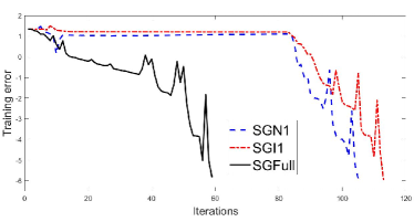
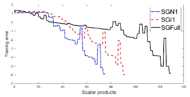
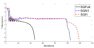
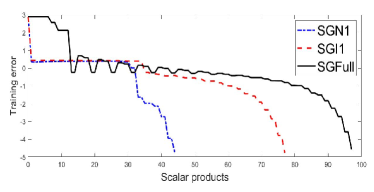
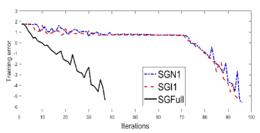
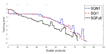
In Figures 3-5 we plot the training loss versus iterations on the left and versus scalar products on the right. The reported figures refer to a specific run out of $100$ runs, representative of the average behavior of the methods. Plots are in logarithmic scale on the $y$-axes. As expected, for all the three datasets, the spectral gradient method without subsampling requires a much smaller number of iterations with respect to SG_N_1 and SG_I_1. Let us now consider the number of scalar products. Concerning CINA0 and MNIST dataset, both the subsampled methods are less expensive than SGFull, that is, they produce the same training error with a smaller number of scalar products. Moreover, the nested method SG_N_1 appears to be better than the non-nested one. Regarding the Mushrooms dataset, we have that SG_N_1 and SG_I_1 appear to behave very similarly and they are both less efficient than SGFull, therefore on this particular dataset the subsampling scheme does not seem to be convenient with respect to the method without subsampling. This is due to the fact that the size of the training set is small and therefore the gain obtained reducing the sample size is not enough to produce an overall saving.

We also notice that we do not expect an advantage in using the subsampling in all the situations where problems are easy enough (because the starting point is close to the solution, or due to the particular form of the functions $f_{j}$) to be solved by SGFull within a small number of iterations.

4.4 Validation Loss

In the previous subsections we tested the behavior of the Algorithm 2.2 using the deterministic stopping criterion - the norm of the full gradient. Then, we always reach the full sample and ask for an $\epsilon$-accurate first-order method. However, in these applications a reasonable value of the validation error is needed rather than an accurate approximation of the minimizer of (25).

In order to do that, we show numerical results obtained using a stopping criterion related to the validation loss rather than to the training loss or to the full gradient. Notice that the testing data set is usually much smaller than the training set, in our runs it is constituted by the $5$% of samples of the whole dataset. Letting

$$f_{\mathcal{V}{}}(x)=\frac{1}{|\mathcal{V}|}\sum_{j\in{\cal{V}}}f_{j}(x),$$

be the validation loss, we stop whenever the following condition is met:

$$f_{\mathcal{V}}(x_{k})>1.1f_{\mathcal{V}}(x_{k-1})\mbox{ or }|f_{\mathcal{V}}(x_{k-1})-f_{\mathcal{V}}(x_{k}))|<10^{-3}|f_{\mathcal{V}}(x_{k}))|$$ (27)

provided that $N_{k}\geq pN$, with $p\in(0,1)$. Thus, we stop whenever we monitor a 10% increase or a stallation of the validation loss, provided that the sample size is at least a fixed percentage of the full sample size.

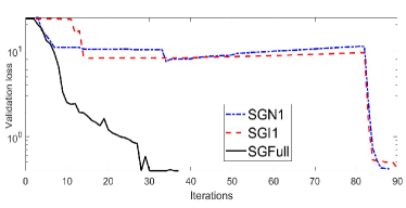
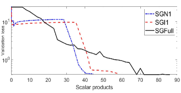
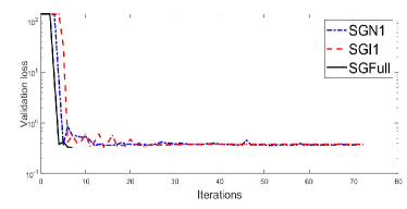
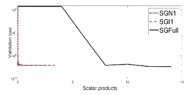
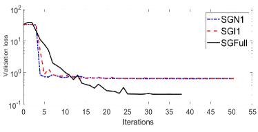
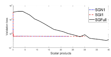
In Figures 6-7 we plot the validation loss versus iterations and scalar products for both SG_N_1 and SG_I_1 using logarithmic scale on the $y$-axes. For the sake of comparison we also plot the validation loss of SGFull stopped when the norm of the gradient is smaller than $10^{-4}$. This way we give a clear indication of the value of the validation loss that can be obtained by a method computing a $10^{-4}$-accurate first-order critical point. The reported figures refer to a specific run out of $100$ runs, representative of the general behavior of the methods. As a first comment we observe that in case of CINA0 dataset, we needed to reach the full sample in order to provide a validation error of the same order of that provided by SGFull. Therefore, for CINA0 dataset, we use $p=1$ in (27). In fact, we can observe that the validation decreases in the very early stage of the iterative process, then it remains almost constant, and then rapidly drops to $0.4$ as soon as the full sample is reached. However, notice that only a very few iterations are performed using the full sample as the average number of iterations is $86$ for SG_N_1 and $90$ for SG_I_1. Notice that the full sample is reached at iteration $82$. On the other hand, considering Mushrooms and MNIST datasets a smaller number of samples are enough to provide an acceptable validation error. Thus, we set $p=0.1$ in (27). In case of Mushrooms the average sample size at termination is $1164$ and $1234$ for SG_N_1 and SG_I_1, respectively. Both methods used around 25% of samples and reached a validation loss value of the order of $0.6$ while SGFull reaches a value of about $0.3$. Analogous behaviour can be observed in the solution of MNIST problem where the average sample size at termination is $7179$ and $6520$ for SG_N_1 and SG_I_1, respectively. Then, the 10% of samples are enough for this dataset.

Figure 6: CINA0 dataset, validation loss versus iterations (left) and versus scalar products (right), stopping criterion (27) with $p=1$

Figure 7: MNIST dataset, validation loss versus iterations (left) and versus scalar products (right), stopping criterion (27) with $p=0.1$

Figure 8: Mushrooms dataset, validation loss versus iterations (left) and versus scalar products (right), stopping criterion (27) with $p=0.1$

5 Conclusions

We analyzed subsampled spectral gradient methods for solving large sum optimization problems with continuously-differentiable objective function. Our main aim was to provide initial understanding of the behavior of such methods with different kinds of spectral coefficients, or more precisely, with different kinds of gradient difference calculations used for obtaining spectral coefficients within the growing sample size framework.

Although the safeguards for the spectral coefficients provide a descent direction regarding the current approximate function, globalization strategy relies on nonmonotone line search. The motivation for this is twofold - to the best of our knowledge, both spectral gradient methods and subsampling methods favor nonmonotone line search techniques. Moreover, if the objective function is assumed to be strongly convex, R-linear convergence is achieved. We provided complexity results for both convex and non-convex case. Further modifications of this approach could be devised in order to solve optimization problems arising in the training of neural network employing non-smooth activation functions.

According to the tests performed on three binary classification problems, our main conclusions are as the following: 1) nested (cumulative) samples perform better than non-nested ones considering costs of the algorithm in terms of scalar products; 2) employing the same subset ${\cal N}_{k}$ for computing the displacement vector $y_{k}$ proved to be beneficial despite the needed additional cost; 3) subsampling seems to reduce the overall computational cost as the tested subsampling variants outperform the full spectral gradient methods except in Mushrooms dataset where the size of the training set is small.

Finally, investigating on the validation loss, we conclude that a mini-batch version of the proposed spectral gradient methods has a good potential. However, stopping criterion in this setting is a problem itself and it needs further analysis. A related question is how the proposed methods compete in the unbounded sample case. This will be one of the topics of our further research.

References

- [1] Causality workbench team, a marketing dataset. http://www.causality.inf.ethz.ch/data/CINA.html, 2008.
- [2] J. Barzilai and J. M. Borwein. Two-point step size gradient method. IMA J. Numerical Analysis, 8(1):141–148, 1988.
- [3] S. Bellavia, G. Gurioli, and B. Morini. Theoretical study of an adaptive cubic regularization method with dynamic inexact hessian information. arXiv:1808.06239, 2018.
- [4] Stefania Bellavia, N. Krejić, and N. Krklec Jerinkić. Subsampled inexact newton methods for minimizing large sums of convex functions. IMA J. Numerical Analysis, 2019.
- [5] A.S. Berahas, R. Bollapragada, and J. Nocedal. An investigation of newton-sketch and subsampled newton methods. arXiv:1705.06211v3, 2018.
- [6] E. G. Birgin, J. M. Martínez, and Marcos Raydan. Spectral projected gradient methods: Review and perspectives. Journal of Statistical Software, 60, 2014.
- [7] E.G. Birgin, N. Krejić, and J.M. Martínez. On the employment of inexact restoration for the minimization of functions whose evaluation is subject to programming errors. Mathematics of Computation, 87:1307–1326, 2018.
- [8] D. Blatt, A. O. Hero, and H. Gauchman. A convergent incremental gradient method with a constant step size. SIAM Journal of Optimization, 18(1):29–51, 2007.
- [9] R. Bollapragada, R. R. Byrd, and J. Nocedal. Exact and inexact subsampled newton methods for optimization. IMA Journal Numerical Analysis, 2018.
- [10] L. Bottou. Stochastic gradient learning in neural networks. Proceedings of Neuro-Nimes, 91(8):12, 1991.
- [11] L. Bottou, F. E. Curtis, and J. Nocedal. Optimization methods for large-scale machine learning. SIAM Review, 60(2):223–311, 2018.
- [12] R.H. Byrd, G.M. Chin, J. Nocedal, and Y. Wu. Sample size selection in optimization methods for machine learning. Mathematical Programming, 134(1):127–155, 2012.
- [13] Y. H. Dai, W. W. Hager, K. Schittkowski, and H. Zhang. The cyclic barzilai-borwein method for unconstrained optimization. IMA Journal Numerical Analysis, 26(3):604–627, 2006.
- [14] Daniela di Serafino, Valeria Ruggiero, Gerardo Toraldo, and Luca Zanni. On the steplength selection in gradient methods for unconstrained optimization. Applied Mathematics and Computation, 318:176–195, 2006.
- [15] R. Fletcher. On the barzilai-borwein gradient method. In L. Qi, K. Teo, and X. Yang, editors, Optimization and Control with Applications, Applied Optimization, volume 96, pages 235–256. Springer, 2005.
- [16] M. P. Friedlander and M. Schmidt. Hybrid deterministic-stochastic methods for data fitting. SIAM Journal on Scientific Computing, 34(3):1380–1405, 2012.
- [17] G. N. Grapiglia and E.W. Sachs. On the worst-case evaluation complexity of nonmonotone line search algorithms. Computational Optimization and applications, 68(3):555–577, 2017.
- [18] R. Johnson and T. Zhang. Accelerating stochastic gradient descent using predictive variance reduction. Advances in Neural Information Processing Systems, 2013.
- [19] N. Krejić and N. Krklec Jerinkić. Nonmonotone line search methods with variable sample size. Numerical Algorithms, 68(4):711–739, 2015.
- [20] N. Krejić and N. Krklec Jerinkić. Spectral projected gradient method for stochastic optimization. Journal of Global Optimization, 73:59–81, 2018.
- [21] D. H. Li and M. Fukushima. A derivative-free line search and global convergence of broyden-like method for nonlinear equations. Optimization Methods and Software, 13(3):181–201, 2000.
- [22] M. Lichman. Uci machine learning repository. https://archive.ics.uci.edu/ml/index.php, 2013.
- [23] M. Raydan. The barzilai and borwein gradient method for the large scale unconstrained minimization problem. SIAM Journal Optimization, 7(1):26–33, 1997.
- [24] F. Roosta-Khorasani and M.W. Mahoney. Sub-sampled newton methods. Mathematical Programming, 174:293–326, 2019.
- [25] N. N. Schraudolph, J. Yu, and S. Günter. A stochastic quasi-newton method for online convex optimization. SAIS International Conference on Artificial Intelligence and Statistics, pages 436–443, 2007.
- [26] C. Tan, S. Ma, Y. H. Dai, and Y. Qian. Barzilai-borwein step size for stochastic gradient descent. Advances in Neural Information Processing Systems, 29:685–693, 2016.
- [27] Zhuang Yang, Cheng Wang, Zhemin Zhang, and Jonathan Li. Random barzilai-borwein step size for mini-batch algorithms. Engineering Applications of Artificial Intelligence, 72:124–135, 2018.