An interacting holographic dark energy model within an induced gravity brane

Abstract

In this paper, we present a model for the late-time evolution of the universe where a dark energy-dark matter interaction is invoked. Dark energy is modeled through an holographic Ricci dark energy component. The model is embedded within an induced gravity brane-world model. For suitable choices of the interaction coupling, the big rip and little rip induced by the holographic Ricci dark energy, in a relativistic model and in an induced gravity brane-world model, are removed. In this scenario, the holographic dark energy will have a phantom-like behaviour even though the brane is asymptotically de Sitter.

I Introduction

Recent astrophysical observations of type Ia supernovae (SNIa) Perlmutter:1998np , cosmic microwave background (CMB) Komatsu:2010fb , large scale structure (LSS) Tegmark2004 , and the recent Planck measurements Planck , suggest that our universe is undergoing an era of accelerated expansion. Quantitative analysis shows that there is a dark energy component (DE) with a negative pressure component leading to the current accelerating expansion of the Universe. Since the fundamental origin and nature of such a dark energy remain enigmatic at present, various models of dark energy have been put forward, such as a small positive cosmological constant Peebles and several kinds of scalar fields like quintessence Ratra , k-essence ARMENDARIZ-PICON2001 , phantom Caldwell , etc. Furthermore, the price of explaining the current cosmic acceleration by DE is the appearence of future singularities at late-time Universe. While some singularities like a big rip (BR) Caldwell , sudden singularities Noj ; Bar , big freeze singularities Bouh3 and big brake singularities Chim1 ; Cata could happen at a finite cosmic time, others abrupt which are events smoother like a little rip (LR) Ruz ; Noj2 ; Stef ; Bouh1 ; Fram ; Bre ; Bouh2 , a little sibling of a BR Yas1 , a little bang and a little sibling of big bang Yas2 could happen at a infinite cosmic time.

Currently, another model inspired by the holographic principle has been put forward to explain the current cosmic acceleration, which states that the number of degrees of freedom for a system within a finite region should be finite and bounded by the area of its boundary 'tHooft:1993gx ; Susskind:1994vu . It is commonly believed that the holographic principle 'tHooft:1993gx ; Susskind:1994vu ; Bekenstein is a fundamental principle of quantum gravity. Based on an effective quantum field theory, Cohen et al. Cohen:1998zx pointed out that, for a system with size L, which is not a black hole, the quantum vacuum energy of the system should not exceed the mass of the same size black hole, i.e. $L^{3}\rho_{\Lambda}\leq LM_{p}^{2}$, where $\rho_{\Lambda}$ is the vacuum energy density fixed by UV cutoff $\Lambda$ and $M_{p}$ denotes the Plank mass. The largest IR cutoff $L$ is chosen by saturating the inequality Li:2004rb ; Hsu:2004ri so that we get the holographic energy density $\rho_{H}=3c^{2}M_{p}^{2}/L^{2}$, where $c$ is a numerical factor. Later on and for convenience, we will instead use the parameter defined as $\beta=c^{2}$. The holographic dark energy model is based on applying the previous ideas to the universe as a whole with the goal of explaining the current speed up of the universe. Then, the IR cutoff can be taken as a cosmic scale of the universe, like the Hubble horizon Li:2004rb ; Hsu:2004ri , particle horizon, event horizon Li:2004rb or second order geometrical invariants luongo1 . Another choice for the IR cutoff L was suggested by Gao et al. Gao (see also NojiriGRG2006 ), in which the IR cutoff of the holographic dark energy (HDE) is taken to be the Ricci scalar curvature. Being an invariant quantity, the Ricci scalar curvature has many particularities such as its cosmological implications in describing the HDE Yas2 ; Gao ; NojiriGRG2006 ; OualiPRD85 , its space-time dependence and its advantages in avoiding the fine tuning and the causality problems Li:2004rb . For all these reasons we will choice the Ricci scalar as the holographic cutoff.

Another approach to explain the observed acceleration of the late universe is based on alternative theory of general relativity like the one inspired by string theory such as the brane-world scenario. The induced gravity brane-world model proposed by Dvali, Gabadadze, and Porrati (DGP) is well known and studied Dvali:2000hr . It contains two branches Deffayet:2000uy the self accelerating branch which suffers from some problems and the normal branch. Even though the normal branch is healthy it cannot describe the current acceleration of the universe unless a dark energy component is invoked Sahni ; Zhang or the gravitational action is modified BouhmadiLopez:2010pp . In the context of the DGP scenario, different models have been studied with various kind of sources for DE in Refs jawad ; dutta ; Rav ; far ; she ; gha ; Shtanov1 .

Furthermore, in the context of the dark sector, one of the main problem raised and without explanation in the framework of $\Lambda$CDM cosmology is the cosmic coincidence problem, i.e. why dark energy density is of the same order of magnitude as cold dark matter energy density (CDM). An interacting mechanism between these two components could alleviate the cosmic coincidence problem as suggested by several authors Bouhmadi-Lopez:2016dcs ; Morais:2016bev ; AmendolaPRD62 ; BoehmerPRD78 ; ChenPRD78 ; PavonPLB628 ; CampoPRD78 ; DuranPRD83 ; Rav . These kind of interactions have been invoked in AbdallaPRD95 in order to explain the possible departure from the $\Lambda$CDM model as measured recently by the experiment of the BOSS delubacAA574 for a value of the Hubble parameter at redshift $z=2.34$. In Ref. OualiPRD85 , we pointed out that the normal branch when filled with an holographic Ricci dark energy (HRDE) can face some DE singularities. This motivated us to improve the model with the aim to remove or smooth these singularities by introducing an interaction between the HDE density and the CDM sector. An interaction between DE and CDM can relieve the coincidence problem and at the same time may smooth some DE singularities.
Recently, interactions between DE and CDM in the holographic model have received a great interest by choosing the infrared cutoff as the Hubble scale PavonPLB628 ; shey , as the future event horizon WangPLB624 , as the Granda and Oliveros scale jawad , as a Ricci scale Yas2 and as a modified holographic DE Chim2 ; Chim3 We show that this kind of interaction is also a promising way to avoid or to smooth the big rip and the little rip appearing in the non interacting models Li:2004rb ; Hsu:2004ri ; OualiPRD85 ; BouhmadiPRD84 .

The unknown nature of DE and CDM makes difficult and imprecise the choice of the form of the interaction between them. However, the interaction is usually considered from a phenomenological point of view WangPLB624 ; GuoPRD76 ; OlivaresPRD74 ; Wang:2016lxa , from the outset given in PavonPLB628 ; CampoPRD78 or from thermodynamical consideration WangPLB662 ; PavonGRG41 . The conservation equations have dimensions of energy density divided by unit of time, therefore, the interaction between DE and CDM is expected to lead precisely to this kind of terms on the right hand side (rhs) of their respective continuity equations, i.e. functions of the energy densities of DE and CDM multiplied by a quantity with units inverse of time such as the Hubble scale as have been widely discussed in Refs WangPLB624 ; GuoPRD76 ; WangPLB637 ; PavonPLB628 ; CampoPRD74 ; CampoPRD71 ; OlivaresPRD74 . The cosmological perturbations in this kind of models have been studied in HePLB . It was shown in that work that if the energy density of DE is phantom like, the curvature perturbations are always stable no matter if the coupling is proportional to DE density or to CDM energy density. However, it was shown that if dark energy is of a quintessence nature, the curvature perturbations are unstable unless the coupling of the interaction is proportional to DE density and the range of the coupling takes some specific values.

Motivated by the study of Refs. HePLB ; AbdallaPRD95 , we consider as well this form of interaction i.e. $Q=\lambda_{m}H\rho_{m}$, $Q=\lambda_{H}H\rho_{H}$, or $Q=H(\lambda_{m}\rho_{m}+\lambda_{H}\rho_{H})$ where $Q$ denotes the interaction between the energy densities $\rho_{m}$ of CDM and the HRDE component $\rho_{H}$. The range of the coupling of the interaction, $\lambda_{m}$ and $\lambda_{H}$, are determined by observations HePRD83 ; FengPLB665 . Considering that there is only energy transfer between DE and CDM, the energy transfer is from CDM to DE if $Q<0$ or from DE to CDM if $Q>0$ (see Eqs. (1) and (2)).

The main aim of this paper is to show that an interacting holographic Ricci dark energy (IHRDE) with CDM can describe suitably the late-time acceleration of the universe, and at the same time improves the model without interaction by avoiding the big rip and/or little rip happening in the model we studied in Ref. OualiPRD85 .

The outline of this paper is as follows. In Sec. II we briefly present an interacting CDM-HRDE model within a DGP brane-world model. We assume that the Ricci scalar is the IR cutoff of the holographic energy density. In Sec. III, we study the modified Friedmann equation without a bulk Gauss-Bonnet (GB) term by analyzing analytically the asymptotic behavior of the brane and numerically the whole expansion of the brane. An appropriate choice of the interaction coupling $\lambda_{H}$ avoids the big rip and the little rip from the normal branch and hence the IHRDE gives a satisfactory and an alternative description of the late time cosmic acceleration of the universe as compared with the HRDE without the GB term in the bulk in the absence of interaction. Indeed the later one modifies the big rip and little rip into a big freeze one while the former removes them definitively. In Sec. IV, we consider the model where the bulk contains a GB term. In this case the asymptotic behaviour of the IHRDE model depends on the sign of a discriminant ${\mathcal{D}}$ which depends on the holographic parameter $\beta$, the GB term, and the coupling $\gamma$ (see Eqs. (44)-(46)). The IHRDE model succeed in removing the big rip and little rip from the future evolution of the brane. On this case, the brane will evolve asymptotically as a de Sitter universe for $\gamma=\frac{1}{2\beta_{\lim}}$, while for $\gamma\neq\frac{1}{2\beta_{\lim}}$, the situation becomes more complicated and depends on the values of the holographic parameter as well as on the interaction parameter. At this regard, as we will show that the coupling between HRDE and CDM plays a crucial role, even more important than the GB parameter, in removing the future singularities. Finally, in Sec. V, we conclude.

II  INTERACTING MODEL AND PARAMETER CONSTRAINTS

We consider a DGP brane-world model, where the bulk contains a GB curvature term, and the brane contains an induced gravity term on its action Kofinas:2003rz ; BouhmadiLopez:2008nf . We restrict our analysis to the normal branch. Assuming only an interaction between CDM and the holographic component on the brane, the conservation equations of the energy density read

$$\overset{\cdot}{\rho}_{\mathrm{H}}+3H(1+\omega_{\mathrm{H}})\rho_{\mathrm{H}} = -Q$$ (1)

$$\overset{\cdot}{\rho}_{\mathrm{m}}+3H\rho_{\mathrm{m}} = Q.$$ (2)

where $H$  is the Hubble parameter and $\omega_{\mathrm{H}}$ denotes the equation of state parameter of the holographic dark energy component.

The modified Friedmann equation in the normal branch of the DGP brane world universe containing an holographic Ricci dark energy, $\rho_{H}$, and a CDM component, with energy density $\rho_{m}$, can be written as Kofinas:2003rz ; BouhmadiLopez:2008nf ; richard

$$H^{2}=\frac{1}{3M_{p}^{2}}\rho-\frac{1}{r_{c}}\left(1+\frac{8\alpha}{3}H^{2}\right)H,$$ (3)

where $\rho=\rho_{\mathrm{m}}+\rho_{\mathrm{H}}$ is the total cosmic fluid energy density of the brane. The parameter $r_{c}$ is the cross-over scale which determines the transition from a 4-dimensional (4D) to a 5-dimensional (5D) behaviour, and $\alpha$ is the Gauss-Bonnet parameter.

Furthermore, for a spatially flat Friedmann-Lemaître-Robertson-Walker universe, the Ricci scalar curvature is given by

$$\mathcal{R=}-6\left(\dot{H}+2H^{2}\right),$$ (4)

the dot stands for the derivative with respect to the cosmic time of the brane.

As already mentioned in the introduction, $\rho_{\mathrm{H}}$ is related to the UV cutoff, while $L$ is related to the IR cutoff. Identifying $L^{-2}$ with $-\mathcal{R}/6,$ the energy density of the HRDE is given by Gao ; OualiPRD85

$$\rho_{\mathrm{H}}=3\beta M_{P}^{2}\left(\frac{1}{2}\frac{dH^{2}}{dx}+2H^{2}\right),$$ (5)

where $x=\ln(a/a_{0})$. The quantities $a$, $a_{0}$ and $\beta=c^{2}$ are respectively the scale factor, its present value and the holographic dimensionless parameter which, as we will show, plays a significant role in determining the asymptotic behavior of the HRDE and therefore of the brane evolution. From now on, the subscript 0 stands for quantities evaluated at the present time.

The modified Friedmann equation (3) can be further rewritten as:

$$E^{2}=\Omega_{\mathrm{m}}+\Omega_{\mathrm{H}}-2\sqrt{\Omega_{\mathrm{r_{c}}}}(1+\Omega_{\mathrm{\alpha}}E^{2})E,$$ (6)

where $E(z)=H/H_{0}$, $z$ is the redshift and

$$\Omega_{\mathrm{m}} = \frac{\rho_{\mathrm{m}}}{3M_{p}^{2}H_{0}^{2}},\,\,\,\,\Omega_{\mathrm{r_{c}}}=\frac{1}{4r_{\mathrm{c}}^{2}H_{0}^{2}},\text{\thinspace\ }$$ (7)

$$\,\Omega_{\mathrm{\alpha}} = \frac{8}{3}\alpha H_{0}^{2},$$ (8)

$$\text{\ }\Omega_{\mathrm{H}} = \beta(\dfrac{1}{2}\dfrac{dE^{2}}{dx}+2E^{2}).$$ (9)

The cosmological parameters of the model are constrained by evaluating the Friedmann equation (6) at present

$$1=\Omega_{\mathrm{m}_{0}}+\Omega_{\mathrm{H}_{0}}-2\sqrt{\Omega_{r_{c}}}(1+\Omega_{\mathrm{\alpha}}),$$ (10)

i.e. $E(x=0)=1$. By combining this equation and Eq. (9) we obtain:

$$\frac{dE}{dx}\Big{|}_{x=0}=-2+\frac{\Omega_{\mathrm{H}_{0}}}{\beta}\text{,}$$ (11)

On the other hand, given that the universe is currently accelerating the present value of the deceleration parameter, $q=-(1+d\ln E/dx)$, which reads:

$$q_{0}=1-\frac{\Omega_{\mathrm{H}_{0}}}{\beta}.$$ (12)

must be negative, therefore

$$0<\beta=\frac{1-\Omega_{\mathrm{m}_{0}}+2\sqrt{\Omega_{rc}}(1+\Omega_{\mathrm{\alpha}})}{1-q_{0}}<\Omega_{\mathrm{H}_{0}}.$$ (13)

As we mentioned in the introduction, the following analysis will be devoted to the normal branch because it requires dark energy and because it is free from the theoretical problems plugging the self-accelerating branch. By using the constraint (10), it can be shown that the holographic parameter $\beta$ verifies

$$\frac{1-\Omega_{\mathrm{m}_{0}}}{1-q_{0}}<\frac{1-\Omega_{\mathrm{m}_{0}}+2\sqrt{\Omega_{rc}}}{1-q_{0}}<\beta.$$ (14)

Taking into account the latest Planck data Planck : $\Omega_{\mathrm{m}_{0}}\sim{0.315}$ and $q_{0}\sim-0.558$, therefore the ratio $\beta_{\textrm{lim}}\doteq\frac{1-\Omega_{\mathrm{m}_{0}}}{1-q_{0}}$ is of the order $0.44$, which means that the normal branch is characterized by $0.44<\beta$.

From equations (6) and (9) the variation of the dimensionless Hubble rate $E$ with respect to $x$ is

$$\dfrac{dE^{2}}{dx}=-\frac{2\Omega_{m}+2(2\beta-1)E^{2}-4\sqrt{\Omega_{r_{c}}}(1+\Omega_{\alpha}E^{2})E}{\beta}$$ (15)

On the other hand, the energy conservation equation (2) gives

$$\dfrac{d\Omega_{m}}{dx}+3\Omega_{m}=\lambda_{H}\Omega_{H}+\lambda_{m}\Omega_{m}.,$$ (16)

Then, using Eq. (9) we obtain

$$\dfrac{d\Omega_{m}}{dx}=\lambda_{H}\left(\dfrac{\beta}{2}\dfrac{dE^{2}}{dx}+2\beta E^{2}\right)+\left(\lambda_{m}-3\right)\Omega_{m},$$ (17)

and with Eq. (15)  we get

$$\dfrac{d\Omega_{m}}{dx} = \Big{[}2\lambda_{H}\beta-\left(2\beta-1\right)(\lambda_{m}-3)\Big{]}E^{2}$$

$$+ \Big{[}\lambda_{H}\beta-\beta(\lambda_{m}-3)\Big{]}E\dfrac{dE}{dx}$$

$$+2 \sqrt{\Omega_{r_{c}}}(\lambda_{m}-3)(1+\Omega_{\alpha}E^{2})E,$$

The derivative of equation (15) gives

$$\dfrac{d^{2}E^{2}}{dx^{2}} = -\frac{2}{\beta}\dfrac{d\Omega_{m}}{dx}-\frac{2\left(2\beta-1\right)}{\beta}\dfrac{dE^{2}}{dx}$$ (19)

$$+ \frac{4\sqrt{\Omega_{r_{c}}}}{\beta}(1+3\Omega_{\alpha}E^{2})\dfrac{dE}{dx}$$

Finally, by using Eq. (II), we have

$$\dfrac{d^{2}E^{2}}{dx^{2}} = \Big{[}-\lambda_{H}+(\lambda_{m}-3)-2\frac{\left(2\beta-1\right)}{\beta}\Big{]}\dfrac{dE^{2}}{dx}$$

$$+2 \Big{[}-2\lambda_{H}+\frac{\left(2\beta-1\right)(\lambda_{m}-3)}{\beta}\Big{]}E^{2}$$

$$+ \frac{4\sqrt{\Omega_{r_{c}}}}{\beta}(1+3\Omega_{\alpha}E^{2})\dfrac{dE}{dx}$$

$$- \frac{4\sqrt{\Omega_{r_{c}}}(\lambda_{m}-3)}{\beta}(1+\Omega_{\alpha}E^{2})E$$

In the absence of interaction, i.e. for $\lambda_{H}=\lambda_{m}=0$, the model coincides with that of Ref. OualiPRD85 , in which we have shown that for $\Omega_{\alpha}=0$, the HRDE will have a phantom-like behaviour until it reaches a big rip singularity for $\beta<1/2$ and a little rip for $\beta=1/2$. In our present model, in which the interaction between CDM and HRDE is included, we can show numerically that the little rip for $\beta=1/2$, and the big rip for $\beta_{\lim}<\beta<1/2$ can be avoided which in the previous work OualiPRD85 becomes a big freeze by including a GB term in the bulk action. The question that now arises is for which values of $\lambda_{H}$, $\lambda_{m}$ and $\beta$ these singularities appearing in that model can be avoided? To answer this question, we notice that the differential equation (II) is not linear so it is not easy to solve analytically. However, our numerical analysis of Eq. (II) shows that its asymptotic behaviour is the same as the one of Eqs. (II) with ${d\Omega_{m}}/{dx}=0$ i.e. in the far future $\Omega_{m}$ as well as ${d\Omega_{m}}/{dx}$ can be neglected. This simplify considerably our task with respect of the above singularities.

III Model without a Gauss-Bonnet term

In order to solve equation (II), we consider first the model without a bulk Gauss-Bonnet term i.e. $\Omega_{\alpha}=0$, therefore

$$\dfrac{d^{2}E^{2}}{dx^{2}} = \Big{[}-\lambda_{H}+(\lambda_{m}-3)-2\frac{\left(2\beta-1\right)}{\beta}\Big{]}\dfrac{dE^{2}}{dx}$$ (21)

$$+ 2\Big{[}-2\lambda_{H}+\frac{\left(2\beta-1\right)(\lambda_{m}-3)}{\beta}\Big{]}E^{2}$$

$$+ \frac{4\sqrt{\Omega_{r_{c}}}}{\beta}\dfrac{dE}{dx}-\frac{4\sqrt{\Omega_{r_{c}}}(\lambda_{m}-3)}{\beta}E$$

and we can write the equation (II) as

$$\left[\lambda_{H}\beta-\beta(\lambda_{m}-3)\right]\dfrac{dE}{dx}$$

$$= -\left[2\lambda_{H}\beta-\left(2\beta-1\right)(\lambda_{m}-3)\right]E-2\sqrt{\Omega_{rc}}(\lambda_{m}-3)$$

In the following, we will discus the solution to the above equation for the model $Q=\lambda_{\mathrm{m}}H\rho_{\mathrm{m}}$, $Q=\lambda_{\mathrm{H}}H\rho_{\mathrm{H}}$, and $Q=\lambda_{\mathrm{m}}H\rho_{\mathrm{m}}+\lambda_{\mathrm{H}}H\rho_{\mathrm{H}}.$

III.1 The model $Q=\lambda_{\mathrm{m}}H\rho_{\mathrm{m}}$

This model corresponds to $\lambda_{H}=0$ and can be split in two cases. The case $\lambda_{m}=3$ which implies, from Eq. (II), that $\Omega_{m}$ is always constant. This case is not physically acceptable as DM behaves as a cosmological constant. And the case $\lambda_{m}\neq 3$ where the holographic parameter plays a crucial role in determining the asymptotic behaviour of the brane:

III.1.1  Asymptotic behavior $\beta=1/2$

There is a unique solution corresponding to little rip solution supported by the normal branch

$$E=4\sqrt{\Omega_{rc}}x+C_{1},$$ (23)

where $C_{1}$ is a constant of integration.

III.1.2 Asymptotic behavior $\beta\neq 1/2$:

Equation (III) gives the solution

$$\left|\left(2\beta-1\right)E-2\sqrt{\Omega_{r_{c}}}\right|$$

$$= \left|\left(2\beta-1\right)E_{1}-2\sqrt{\Omega_{r_{c}}}\right|\exp[-\frac{\left(2\beta-1\right)}{\beta}(x-x_{1})],$$

where $E_{1}$ and $x_{1}$ are integration constants.

• For $\beta>1/2$, the dimensionless Hubble rate reaches a constant value and the brane is asymptotically de Sitter

  $$E_{\infty}=\frac{2}{2\beta-1}\sqrt{\Omega_{rc}}.$$ (25)

  We notice that this asymptotic de Sitter solution is possible only for $\beta\neq 1/2$. On the other hand, we note that equation (16) with $\lambda_{H}=0$, gives the solution $\Omega_{m}=\Omega_{\mathrm{m}_{0}}e^{(\lambda_{m}-3)x},$ and by substituting it in Eq. (6), we conclude that with the finite value of the dimensionless Hubble parameter $E_{\infty}$ of Eq. (25), $\lambda_{m}$ must be less or equal to $3$ to ensure that$\ \Omega_{\mathrm{H}}$ (and therefore $E$) converges asymptotically in the far future to a finite value. So in this case the energy density of CDM is practically zero at the far future, and the universe converges asymptotically to a universe filled exclusively with an HRDE component.

• For $\beta_{\textrm{lim}}<\beta<1/2$, the dimensionless Hubble rate blows up in the far future, and it follows a superaccelerated expansion until it hits a big rip singularity.
  

  Therefore, the IHRDE model with $Q=\lambda_{\mathrm{m}}H\rho_{\mathrm{m}}$ has the same asymptotic behaviour as the model analized in Ref. OualiPRD85 . So we conclude that this model does not succeed in removing the big rip and the little rip singularities happening in the non-interacting model OualiPRD85 .

III.2 The model $Q=\lambda_{\mathrm{H}}H\rho_{\mathrm{H}}$

This model corresponds to $\lambda_{{m}}=0$. The holographic $\beta$ parameter determines the asymptotic behaviour of the brane as follow.

III.2.1 Asymptotic behavior $\beta=\beta_{\mathrm{LR}}\doteq\frac{3}{2(\lambda_{H}+3)}$

In this case Eq. (III) gives a little rip solution:

$$E_{\mathrm{LR}}=4\sqrt{\Omega_{rc}}x+C_{2},$$ (26)

where $C_{2\text{ }}$is an integration constant.

III.2.2 Asymptotic behavior $\beta\neq\beta_{\mathrm{LR}}$

The solution of Eq. (III) is given by:

$$\left|\left[2\lambda_{H}\beta+3\left(2\beta-1\right)\right]E-6\sqrt{\Omega_{rc}}\right|$$

$$= \left|\left[2\lambda_{H}\beta+3\left(2\beta-1\right)\right]E_{1}-6\sqrt{\Omega_{rc}}\right|$$

$$\exp[-\frac{\left[2\lambda_{H}\beta+3\left(2\beta-1\right)\right]}{\beta(\lambda_{H}+3)}(x-x_{1})],$$

where $E_{1}$ and $x_{1}$ are integration constants.

For clarity we divide our analysis in two cases:

1. $\beta<\beta_{\mathrm{LR}}$.

   The dimensionless Hubble rate blows up in the far future, and it follows a super accelerated expansion until it hits a big rip singularity.

2. $\beta>\beta_{\mathrm{LR}}$.

   The brane is asymptotically de Sitter, i.e. the Hubble rate reaches a constant value $E_{\infty}$,

   $$E_{\infty}=\frac{6\sqrt{\Omega_{rc}}}{2\beta\lambda_{H}+3\left(2\beta-1\right)}.$$ (28)

   $E_{\infty}$ must be positive. The condition $E_{\infty}>0$, is directly related to the choice of the parameters of the model as can be seen in Eq. (28). For $\beta=1/2$, the solution reduces to $E_{\infty}=6\sqrt{\Omega_{rc}}/\lambda_{H}$ which is finite and no little rip is reached for a finite $\lambda_{H}$, unless when $\lambda_{H}\longrightarrow 0$, where $E_{\infty}$ blows up and one approaches the model where there is no interaction OualiPRD85 , for which the little rip is inevitable for $\beta=1/2$. For $\beta>1/2$ the asymptotical de Sitter solution $E_{\infty}$ remains even if $\lambda_{H}=0.$

We conclude that the interacting model acts only on the interval $\beta_{\textrm{lim}}<\beta\leq 1/2$ of the normal branch, and by choosing $\beta_{\mathrm{LR}}=\frac{3}{2(\lambda_{H}+3)}<\beta_{\textrm{lim}}$ one can avoid the big rip singularity for $\beta_{\textrm{lim}}<\beta<1/2$ and the little rip for $\beta=1/2$ presents in the model without interaction OualiPRD85 . We notice that the inclusion of interaction between CDM and HRDE gives a satisfactory results as compared with the inclusion of the GB effect in the HRDE model studied in Ref. OualiPRD85 . Indeed, the inclusion of the GB term does not avoid the singularity but it alters it to a big freeze singularity while the interacting model smooth the singularities by an appropriate choose of the limiting value of the holographic parameter.

III.3 The model $Q=\lambda_{\mathrm{H}}H\rho_{\mathrm{H}}+\lambda_{\mathrm{m}}H\rho_{\mathrm{m}}$

III.3.1 $\lambda_{m}=3$

In this case Eq. (III) gives the solution of the dimensionless Hubble rate as

$$E=E_{1}\exp[-2(x-x_{1})],$$ (29)

where $E_{1}$ and $x_{1}$ are integration constants and it is reduced to a Minkowski one at far future.

III.3.2 $\lambda_{H}=(\lambda_{m}-3)$ and $\lambda_{m}\neq 3$

In this case the brane has a negative constant dimensionless Hubble rate and it is not physical at late-time

$$E=-2\sqrt{\Omega_{rc}},$$ (30)

III.3.3 $\lambda_{H}\neq(\lambda_{m}-3)$ and $\lambda_{m}\neq 3$

Asymptotic behavior $\beta=\beta_{\text{LR}}\doteq\frac{3-\lambda_{m}}{2\lambda_{H}-2\lambda_{m}+6}$

We notice that for $\lambda_{m}\neq 3$ and $\lambda_{H}\neq(\lambda_{m}-3)$ the solution leads to a little rip when $\beta=\beta_{\text{LR}}$ and the Hubble parameter reads

$$E=4\sqrt{\Omega_{rc}}x+C_{3},$$ (31)

where $C_{3}$ is a constant of integration.

Asymptotic behavior $\beta\neq\beta_{\text{LR}}$

The solution of Eq. (III) is given by:

$$\left|\left[2\lambda_{H}\beta-\left(2\beta-1\right)(\lambda_{m}-3)\right]E+2\sqrt{\Omega_{rc}}(\lambda_{m}-3)\right|$$ (32)

$$= \left|\left[2\lambda_{H}\beta-\left(2\beta-1\right)(\lambda_{m}-3)\right]E_{1}+2\sqrt{\Omega_{rc}}(\lambda_{m}-3)\right|$$

$$\exp[-\frac{\left[2\lambda_{H}\beta-\left(2\beta-1\right)(\lambda_{m}-3)\right]}{\lambda_{H}\beta-\beta(\lambda_{m}-3)}(x-x_{1})]$$

1. If $\beta>\beta_{\text{LR}}$.

   The asymptotic solution corresponds to a de Sitter brane whose Hubble parameter reads

   $$E_{\infty}=\frac{-2\sqrt{\Omega_{rc}}(\lambda_{m}-3)}{2\lambda_{H}\beta-\left(2\beta-1\right)(\lambda_{m}-3)}.$$ (33)

   This asymptotic de Sitter solution gives a finite asymptotic value of $\Omega_{\mathrm{H}}$ (see Eq. (9)).
   

   Notice that equation (16) can be written in the limit where $\Omega_{\mathrm{H}}$ converges asymptotically to a finite value $\Omega_{\mathrm{H}_{\infty}}$ as $(3-\lambda_{\mathrm{m}})\Omega_{\mathrm{m\infty}}=\lambda_{\mathrm{H}}\Omega_{\mathrm{H}_{\infty}},$ so one can conclude that $\lambda_{m}$ must be always less than $3$ in order to have $\Omega_{\mathrm{m\infty}}>0$.
   

   On the other hand, For $\beta=1/2$ the solution (33) is reduced to $E_{\infty}=\frac{2\sqrt{\Omega_{rc}}(3-\lambda_{m})}{\lambda_{H}}$ which is finite and the little rip is avoided for a finite $\lambda_{H}$. While for $\lambda_{H}\longrightarrow 0$, $E_{\infty}$ blows up. In this case one approaches the model $Q=\lambda_{\mathrm{m}}H\rho_{\mathrm{m}}$ which coincides with the non interaction case OualiPRD85 . For $\beta>1/2$, the asymptotic de Sitter solution $E_{\infty}$ is still present even for $\lambda_{H}=0$ and $\lambda_{m}=0$. For $\beta_{\lim}<\beta<0.5$, $E_{\infty}$ is positive by choosing $\lambda_{H}>\frac{1-2\beta}{2\beta}(3-\lambda_{m})$. Here again by an appropriate choose of $\lambda_{H}$, one can avoid the big rip singularity.

2. $\beta<\beta_{\text{LR}}$. The dimensionless Hubble rate blows up in the future and it follows a super accelerating expansion until it reaches a big rip singularity.
   

As in the previous subsection, we notice that the interaction between CDM and an holographic Ricci dark energy density gives satisfactory results as compared with the inclusion of a Gauss Bonnet term in the bulk OualiPRD85 . Indeed, the inclusion of a (GB) term does not avoid the singularity but it modifies it to a big freeze singularity while the interacting model does. It is worth noticing, from Eqs. (III) and (33), that the results of the model $Q=\lambda_{\mathrm{H}}H\rho_{\mathrm{H}}+\lambda_{\mathrm{m}}H\rho_{\mathrm{m}}$ are similar to those with $Q=\lambda_{\mathrm{H}}H\rho_{\mathrm{H}}$ by making the transformation $\lambda_{H}$ $\longrightarrow\frac{3\lambda_{H}}{3-\lambda_{m}}$ in the model $Q=\lambda_{\mathrm{H}}H\rho_{\mathrm{H}}$.

III.4 Numerical analysis

The analytical solutions of equation (21) are not at all obvious so a numerical analysis is required.

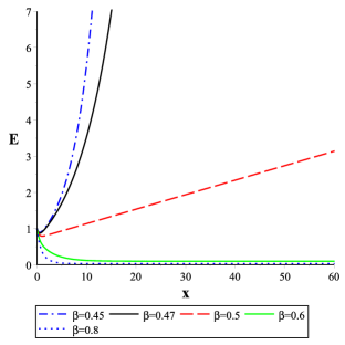
Figure 1:  Plot of the dimensionless Hubble rate $E$ against $x$. The cosmological parameters are assumed to be $\Omega_{m_{0}}=0.315$, $q_{0}=-0.558$, $\lambda_{m}=0.1$ and $\lambda_{H}=0$. The plot has been done for several values of the holographic parameter that are stated at the bottom of the figure.

In order to solve numerically Eq. (21), we choose $\Omega_{m0}=0.315$ and $q_{0}=-0.558$, as it is given by the latest Planck data Planck and assuming that our model is pretty much similar to a $\Lambda$CDM scenario at the present time. For a given value of $\beta$, the dimensionless energy density $\Omega_{H_{0}}$ is fixed through Eq. (12), while the crossover scale parameter $\Omega_{r_{c}}$ is fixed by the constraint Eq. (10).

In Fig. 1, we show the solutions corresponding to the model $Q=\lambda_{\mathrm{m}}H\rho_{\mathrm{m}}$ for different values of $\beta$. For ${\beta=0.45}$ and $\beta=0.47$ the brane expands exponentially with respect to $x$ in the future until it reaches a big rip singularity, while for $\beta=0.6$ and $\beta=0.8$ the brane expands as an inverse of the exponential of $x$ and remains asymptotically de Sitter in the future. Finally for $\beta=0.5$ the brane has an asymptotic solution of the form $E=Ax+B$ which corresponds to a little rip solution. All of these numerical solutions are in agreement with the analytical analysis as it should be. In addition, the model $Q=\lambda_{\mathrm{m}}H\rho_{\mathrm{m}}$ has the same asymptotic result as in Ref. OualiPRD85 .

Figs. 2 and 3 correspond to the model $Q=\lambda_{\mathrm{H}}H\rho_{\mathrm{H}}$. In Fig. 2 we show the numerical solutions of Eq. (21) for different values of $\beta$. For all these solutions the condition $\beta>\frac{3}{2(\lambda_{H}+3)}$ is satisfied, the brane is asymptotically de Sitter in the far future and the dimensionless Hubble rate $E$ approaches the value $E_{\infty}=\frac{6\sqrt{\Omega_{rc}}}{2\beta\lambda_{H}+3\left(2\beta-1\right)}$ which is in agreement with the analytical analysis (see Eq. (28)).

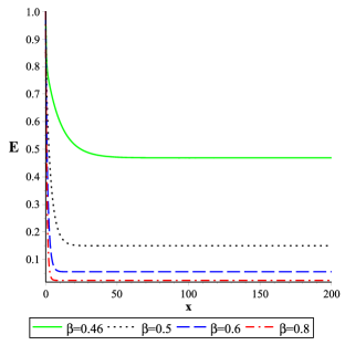
Figure 2: Plot of the dimensionless Hubble rate $E$ against $x$ for the normal branch. The cosmological parameters are assumed to be $\Omega_{m_{0}}=0.315$, $q_{0}=-0.558$, $\lambda_{m}=0$ and $\lambda_{H}=0.4$. The plot has been done for several values of the holographic parameter that are stated at the bottom of the figure.

It is worth noticing the avoidance of the big rip singularity for $\beta_{\textrm{lim}}<\beta<1/2$ and the little rip singularity for $\beta=1/2$ by assuming the interaction between CDM and HRDE component, while in the model OualiPRD85 the big rip and the little rip singularities are obtained respectively for $\beta<1/2$ and $\beta=1/2$. Fig. 3 illustrates the numerical solutions of Eq. (21) for $\beta=0.45$ and for different values of $\lambda_{\mathrm{H}}$. For  $\lambda_{\mathrm{H}}=1/3$, $\lambda_{\mathrm{H}}>\frac{1}{3}$ and $\lambda_{\mathrm{H}}<\frac{1}{3}$, Fig. 3 shows respectively the little rip solution, the de Sitter behaviour and the solution which hits a big rip singularity. For the model $Q=\lambda_{H}H\rho_{H}+\lambda_{m}\rho_{m}$, the above discussions are translated to the sets of the couple $(\lambda_{m},\lambda_{H})$. Indeed, by translating the constraints on $\lambda_{H}$ to $\frac{3\lambda_{H}}{3-\lambda_{m}}$ and requiring that the couple $(\lambda_{m},\lambda_{H})$ verifies these constraints the same conclusions are obtained.

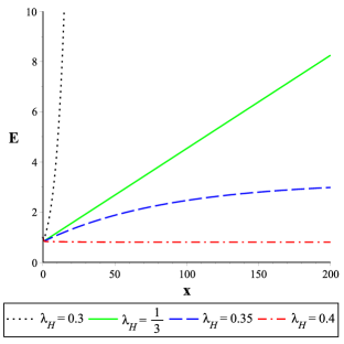
Figure 3: Plot of the dimensionless Hubble rate $E$ against $x$ for the branch $\beta=0.45$. The cosmological parameters are assumed to be $\Omega_{m_{0}}=0.315$, $q_{0}=-0.558$. The plot has been done for $\lambda_{m}=0$ and for several values of the parameter $\lambda_{H}$ that are stated at the bottom of the figure. We can see a big rip behaviour for $\lambda_{H}=0.3$, little rip behaviour for $\lambda_{H}=1/3$ and de Sitter behaviour for $\lambda_{H}\geq 0.35$.

In order to complete our numerical study and by imposing that the brane is currently accelerating, we analyze the equation of state $\omega_{H}=\rm{p}_{H}/\rho_{H}$, $\omega_{\text{eff}}$ and the deceleration parameter $q$ where $\rho_{H}$, $p_{H}$ and $\omega_{\text{eff}}$ are the HRDE density, its pressure and its effective equation of state associated to the effective energy density (please cf. Eq. (3.16)) respectively.

From Eq. (1) and $Q=\lambda_{\mathrm{H}}H\rho_{\mathrm{H}}$, we obtain

$$\omega_{H}=-1-\lambda_{H}-\frac{1}{3}\frac{d\ln(\Omega_{H})}{dx},$$ (34)

where $\Omega_{H}$ is defined in Eq. (9). In terms of the dimensionless Hubble rate E and its derivatives with respect to $x$, $\omega_{H}$ can be rewritten as

$$\omega_{\mathrm{H}}=-\lambda_{\mathrm{H}}-1-\dfrac{\left(\dfrac{dE}{dx}\right)^{2}+E\dfrac{d^{2}E}{dx^{2}}+4E\dfrac{dE}{dx}}{3E\dfrac{dE}{dx}+6E^{2}}.$$ (35)

The effective equation of state $\omega_{\text{eff}}$ can be obtained by rewriting the Friedmann equation (6) as the standard Friedmann equation

$$E^{2}=\frac{1}{3M_{p}^{2}H_{0}^{2}}(\rho_{m}+\rho_{\text{eff}}),$$ (36)

where $\rho_{\text{eff}}$ is the effective energy density that can be defined through Eq. (5) as

$$\rho_{\text{eff}}=3M_{p}^{2}H_{0}^{2}\Big{[}\frac{1}{2}\beta\frac{dE^{2}}{dx}+2\beta E^{2}-2\sqrt{\Omega_{\mathrm{r_{c}}}}E\Big{]}.$$ (37)

Furthermore, from the conservation equation

$$\dot{\rho}_{\text{eff}}+3H(1+\omega_{\text{eff}})\rho_{\text{eff}}=0,$$ (38)

we obtain the effective equation of state

$$1+\omega_{\text{eff}}=-\frac{1}{3\rho_{\text{eff}}}\frac{d\rho_{\text{eff}}}{dx}.$$ (39)

Fig. 4 shows some examples of the behavior of the equation of state for the current cosmological values, for $\lambda_{{H}}=0.1$ and for different values of $\beta$. As it can be clearly noticed from Eq. (35) and illustrated in Fig. 4, $\omega_{H}$ approaches $-\lambda_{\mathrm{H}}-1$ at very late-time for $\beta>\frac{3}{2(\lambda_{H}+3)}$ corresponding to a de Sitter behaviour of the brane as it is also confirmed by the effective equation of state $\omega_{\text{eff}}$ plotted in Fig. 5 (for $\lambda_{\mathrm{H}}=0.1$ and $\beta>0.48$, $\omega_{H}$ approaches $-1.1$ and $\omega_{\text{eff}}$ is less than $-1$). Therefore, HRDE will behave as a phantom like fluid even though the brane undergoes a de Sitter stage asymptotically. Fig. 6 shows that the Universe continues accelerating in the future. For the model $Q=\lambda_{H}H\rho_{H}+\lambda_{m}\rho_{m}$, the sets of the couple $(\lambda_{m},\lambda_{H})$ that verifie the constraint $\frac{3\lambda_{H}}{3-\lambda_{m}}=0.1$ lead to the same conclusions. We conclude that this kind of interaction can describe the current acceleration expansion of our Universe.

IV Model with Gauss-Bonnet term in the bulk

Now we consider the model where the bulk action contains a GB curvature term in order to analyze the possibility of avoiding the big freeze present in the absence of interaction between CDM and HRDE and in order to improve the constraints between the interaction and the beta parameters. In the same manner we show that the avoidance of the big rip and little rip requires finite values of $\Omega_{\mathrm{m}}$ at the far future.

From Eq. (II), the solution for the interaction $\lambda_{\mathrm{m}}=3$ and $\lambda_{H}=0$ is similar to the case without the GB term which is already analysed in the case $Q=\lambda_{\mathrm{m}}H\rho_{\mathrm{m}}$. Therefore, Eq. (II) should be analyzed only for $\lambda_{\mathrm{m}}\neq 3$ and can be written as

$$\Big{[}\lambda_{H}\beta-\beta(\lambda_{m}-3)\Big{]}\dfrac{dE}{dx} = -\Big{[}2\lambda_{H}\beta-\left(2\beta-1\right)(\lambda_{m}-3)\Big{]}E$$

$$- 2 \sqrt{\Omega_{rc}}(\lambda_{m}-3)(1+\Omega_{\alpha}E^{2})$$ (40)

in the asymptotic regime where $d\Omega_{m}/dx\rightarrow 0$.

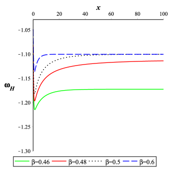
Figure 4: Plot of the equation of state $\omega_{H}$ against $x$ for $\lambda_{H}=0.1$. The cosmological parameters are assumed to be $\Omega_{m_{0}}=0.315$, $q_{0}=-0.558$. The plot has been done for several values of the parameter $\beta$ that are stated at the bottom of the figure.

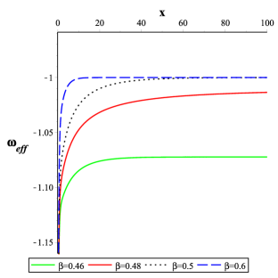
Figure 5: Plot of the effective equation of state $\omega_{\text{eff}}$ against $x$ for $\lambda_{H}=0.1$. The cosmological parameters are assumed to be $\Omega_{m_{0}}=0.315$, $q_{0}=-0.558$. The plot has been done for several values of the parameter $\beta$ that are stated at the bottom of the figure.

For $\lambda_{\mathrm{m}}\neq 3$, and in order to compare our results to the case without interaction OualiPRD85 , it is interesting to rewrite equation (40) as

$$\tilde{\beta}\dfrac{dE}{dx}=-\left[{\left(2\tilde{\beta}-1\right)E-2\sqrt{\Omega_{rc}}(1+\Omega_{\alpha}E^{2})}\right],$$ (41)

where $\tilde{\beta}=\gamma\beta,$ and

$$\ \gamma=\left(1+\frac{\lambda_{H}}{3-\lambda_{m}}\right).$$ (42)

The solutions of Eq. (41) depends on the sign of the discriminant $\mathcal{D}$ of the polynomial on its rhs, which reads

$$\mathcal{D}=\left(2\tilde{\beta}-1\right)^{2}-16\Omega_{r_{c}}\Omega_{\alpha},$$ (43)

and can be factorised as follows

$$\mathcal{D}=\mathcal{F}(\beta-\beta_{-})(\beta-\beta_{+}),$$ (44)

where

$$\beta_{\pm}=\frac{1+\Omega_{\alpha}\pm 2\sqrt{\Omega_{\alpha}}(1-\Omega_{m_{0}})}{2[(1+\Omega_{\alpha})\gamma\pm\sqrt{\Omega_{\alpha}}(1-q_{0})]}.$$ (45)

and

$$\mathcal{F}=4\left[\gamma^{2}-\Omega_{\alpha}\left(\frac{1-q_{0}}{1+\Omega_{\alpha}}\right)^{2}\right].$$ (46)

Fig. 7 shows the behaviour of the parameters $\beta_{\pm}$ against $\Omega_{\alpha}$ for the cosmological parameters $\Omega_{m0}=0.315$ and $q_{0}=-0.558$. As can be seen from Fig. 7, $\beta_{+}=\beta_{-}=\beta_{\textrm{lim}}$ for $\gamma=\frac{1}{2\beta_{\textrm{lim}}}$. For $\frac{1}{2\beta_{\textrm{lim}}}<\gamma$ ($\gamma<\frac{1}{2\beta_{\textrm{lim}}}$), $\beta_{+}<\beta_{-}<\beta_{\textrm{lim}}$ ($\beta_{\textrm{lim}}<\beta_{+}<\beta_{-}$).

In the following we analyze the effect of the interaction between CDM and HRDE component on the singularities appearing on the same model without such interaction (cf. Ref. OualiPRD85 ).

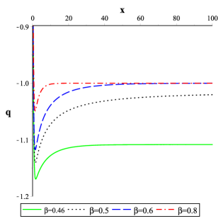
Figure 6: Plot of the deceleration parameter $q$ against $x$ for $\lambda_{H}=0.1$. The cosmological parameters are assumed to be $\Omega_{m_{0}}=0.315$, $q_{0}=-0.558$. The plot has been done for several values of the parameter $\beta$ that are stated at the bottom of the figure.

IV.1 $Q=\lambda_{\mathrm{m}}H\rho_{\mathrm{m}}$

In this case and from Eq. (42) $\gamma=1$, we obtain the same asymptotic result as in Ref. OualiPRD85 , and we conclude, as in the previous section, that the IHRDE model with $Q=\lambda_{\mathrm{m}}H\rho_{\mathrm{m}}$ does not succeed to remove the big freeze presented in the range $\beta_{\lim}<\beta<\beta_{-}$ for the holographic Ricci dark energy in a DGP brane world model with a GB term in the bulk.

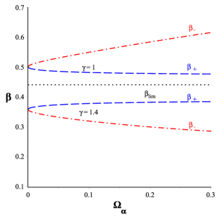
Figure 7: Plot of the $\beta_{\pm}$ parameters against $\Omega_{\alpha}$. The cosmological parameters are assumed to be $\Omega_{m_{0}}=0.315$, $q_{0}=-0.558$. The plot has been done for several values of the parameter $\gamma$.

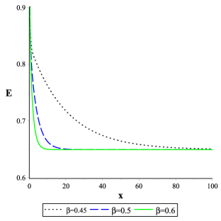
Figure 8: Plot of the dimensionless Hubble rate $E$ against $x$ for an interacting coefficient $\gamma=\frac{1}{2\beta_{\lim}}$. The cosmological parameters are assumed to be $\Omega_{m_{0}}=0.315$, $q_{0}=-0.558$ and $\Omega_{\alpha}=0.1$. The plot has been done for several values of the holographic parameter that are stated at the bottom of the figure.

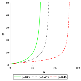
Figure 9: Plot of the dimensionless Hubble rate $E$ against $x$ for the normal branch, and for the negative sign of $\mathcal{D}$. The cosmological parameters are assumed to be $\Omega_{m_{0}}=0.315$, $q_{0}=-0.558$, $\Omega_{\alpha}=0.1$, $\lambda_{m}=0$ and $\lambda_{H}=0.3$. The plot has been done for several values of the holographic parameter that are stated at the bottom of the figure.

IV.2 $Q=\lambda_{\mathrm{H}}H\rho_{\mathrm{H}}$ and $Q=\lambda_{\mathrm{H}}H\rho_{\mathrm{H}}+\lambda_{\mathrm{m}}H\rho_{\mathrm{m}}$

The analysis will be done for the model $Q=\lambda_{\mathrm{H}}H\rho_{\mathrm{H}}$ while the generalization to the model $Q=\lambda_{\mathrm{H}}H\rho_{\mathrm{H}}+\lambda_{\mathrm{m}}H\rho_{\mathrm{m}}$, as it can be noticed from Eq. (III), will be obtained by replacing $\lambda_{H}$ by $\frac{3\lambda_{H}}{3-\lambda_{m}}$

IV.2.1 $\gamma=\frac{1}{2\beta_{\lim}}$

In this case $\beta_{\lim}=\beta_{-}=\beta_{+}$ and the discriminant is equal to $\mathcal{D=}$ $\mathcal{F}(\beta-\beta_{\lim})^{2}$ which is always positive. The solution of the asymptotic Friedmann equation (41) reads:

$$\left|\frac{4\Omega_{\alpha}\sqrt{\Omega_{r_{c}}}E-2\gamma\beta+1+\sqrt{\mathcal{D}}}{4\Omega_{\alpha}\sqrt{\Omega_{r_{c}}}E-2\gamma\beta+1-\sqrt{\mathcal{D}}}\right|=\mathcal{C}_{2}\exp\left[-\frac{\sqrt{\mathcal{D}}}{\gamma\beta}(x-x_{2})\right],$$ (47)

where

$$\mathcal{C}_{2}=\left|\frac{4\Omega_{\alpha}\sqrt{\Omega_{r_{c}}}E_{2}-2\gamma\beta+1+\sqrt{\mathcal{D}}}{4\Omega_{\alpha}\sqrt{\Omega_{r_{c}}}E_{2}-2\gamma\beta+1-\sqrt{\mathcal{D}}}\right|,$$ (48)

$x_{2}$ and $E_{2}$ are integration constants. We can deduce that, for very large values of $x$, the brane behaves asymptotically like an expanding de Sitter universe, i.e. with a constant positive Hubble rate (see Eq. (43))

$$E_{+}=\frac{(2\gamma\beta-1)-\sqrt{\mathcal{D}}}{4\Omega_{\alpha}\sqrt{\Omega_{r_{c}}}}=\frac{(\frac{\beta}{\beta_{\lim}}-1)-\sqrt{\mathcal{D}}}{4\Omega_{\alpha}\sqrt{\Omega_{r_{c}}}}.$$ (49)

IV.2.2 $\gamma\neq\frac{1}{2\beta_{\lim}}$

1. Negative discriminant ($\mathcal{D}<0$): The discriminant $\mathcal{D}$ is negative for $\frac{1}{2\beta_{\lim}}<\gamma$ where $\beta$ satisfies $\beta_{-}<\beta<\beta_{+}<\beta_{\lim}$ or for $\gamma<\frac{1}{2\beta_{\lim}}$ where $\beta_{\lim}<\beta_{+}<\beta<\beta_{-}$ (cf. Eq. (44) and Fig. 7). The first case will be ignored since it corresponds to the self-accelerating branch. Hence only the case $\gamma<\frac{1}{2\beta_{\lim}}$ will be analysed. The Friedmann Eq. (41) can be integrated as

   $$E=\frac{1}{4\Omega_{\alpha}\sqrt{\Omega_{rc}}}\left\{\sqrt{\left|\mathcal{D}\right|}\tan\left[\frac{\sqrt{\left|\mathcal{D}\right|}}{2\gamma\beta}\left(x-\mathcal{C}_{2}\right)\right]+2\gamma\beta-1\right\},$$ (50)

   where

   $$\mathcal{C}_{2}=x_{2}+\frac{2\gamma\beta}{\sqrt{\left|\mathcal{D}\right|}}\arctan\left[\frac{-4\Omega_{\alpha}\sqrt{\Omega_{r_{c}}}E_{2}+2\gamma\beta-1}{\sqrt{\left|\mathcal{D}\right|}}\right],$$ (51)

   $x_{2}$ and $E_{2}$ are integration constants. Consequently, there is always a finite value of the scale factor or $x$ where the Hubble rate and its derivative blow up at

   $$x_{\mathrm{sing_{1}}}=\mathcal{C}_{2}+\frac{2\gamma\beta}{\sqrt{\left|\mathcal{D}\right|}}\left(n+\frac{1}{2}\right)\pi,\quad n\in\mathbb{Z},$$ (52)

   where $"{\mathrm{sing_{1}}}"$ denotes the big freeze singularity. Therefore we conclude that the brane hits a big freeze singularity in the future as the event $x_{\mathrm{sing_{1}}}$ takes place at a finite future cosmic time $t_{\mathrm{sing_{1}}}$ Noj ; BouhmadiLopez:PLB2008 .
   

   

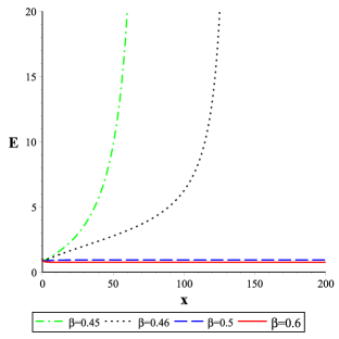
   Figure 10: Plot of the dimensionless Hubble rate $E$ against $x$, for the positive sign of $\mathcal{D}$, and for an interacting coefficient such that $\gamma<\frac{1}{2\beta_{\lim}}$. The cosmological parameters are assumed to be $\Omega_{m_{0}}=0.315$, $q_{0}=-0.558$, $\Omega_{\alpha}=0.1$, $\lambda_{m}=0$ and $\lambda_{H}=0.3$. The plot has been done for several values of the holographic parameter that are stated at the bottom of the figure.

   

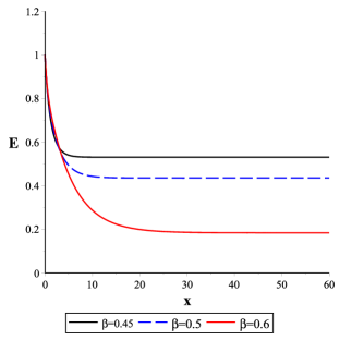
   Figure 11: Plot of the dimensionless Hubble rate $E$ against $x$, for the positive sign of $\mathcal{D}$, and for an interacting coefficient such that $\gamma>\frac{1}{2\beta_{\lim}}$. The cosmological parameters are assumed to be $\Omega_{m_{0}}=0.315$, $q_{0}=-0.558$, $\Omega_{\alpha}=0.1$, $\lambda_{m}=0$ and $\lambda_{H}=0.6$. The plot has been done for several values of the holographic parameter that are stated at the bottom of the figure.

2. Positive discriminant ($0<\mathcal{D}$):

   The discriminant $\mathcal{D}$ is positive for $\frac{1}{2\beta_{\lim}}<\gamma$, and $\beta_{+}<\beta_{\lim}<\beta$ or for $\gamma<\frac{1}{2\beta_{\lim}}$ and $\beta$ satisfying $\beta_{-}<\beta$ or $\beta_{\lim}<\beta<\beta_{+}$ (cf. Eq. (44), Fig. 7, see also Fig. 10, and 11 which will be discussed later).

   The solution of the asymptotic Friedmann equation (41) reads

   $$\left|\frac{4\Omega_{\alpha}\sqrt{\Omega_{r_{c}}}E-2\gamma\beta+1+\sqrt{\mathcal{D}}}{4\Omega_{\alpha}\sqrt{\Omega_{r_{c}}}E-2\gamma\beta+1-\sqrt{\mathcal{D}}}\right|=\mathcal{C}_{2}\exp\left[-\frac{\sqrt{\mathcal{D}}}{\gamma\beta}(x-x_{2})\right],$$ (53)

   where

   $$\mathcal{C}_{2}=\left|\frac{4\Omega_{\alpha}\sqrt{\Omega_{r_{c}}}E_{2}-2\gamma\beta+1+\sqrt{\mathcal{D}}}{4\Omega_{\alpha}\sqrt{\Omega_{r_{c}}}E_{2}-2\gamma\beta+1-\sqrt{\mathcal{D}}}\right|,$$ (54)

   $x_{2}$ and $E_{2}$ are integration constants. We can deduce that the brane behaves asymptotically like an expanding de Sitter universe with a positive Hubble rate

   $$E_{+}=\frac{(2\gamma\beta-1)-\sqrt{\mathcal{D}}}{4\Omega_{\alpha}\sqrt{\Omega_{r_{c}}}},$$ (55)

   for $\gamma>\frac{1}{2\beta}$. While for the case, $\gamma\leq\frac{1}{2\beta}$ the Hubble rate $E_{+}$ is negative and the asymptotic analysis performed is no longer valid. In fact, the brane faces a big freeze singularity where, from Eq. (40), the expansion of the brane can be approximated by

   $$E\sim\frac{\gamma\beta}{2\Omega_{\alpha}\sqrt{\Omega_{r_{c}}}\,(x_{\mathrm{sing_{2}}}-x)}.$$ (56)

   The constant $x_{\mathrm{sing_{2}}}$ stands for the “size” of the brane at this big freeze singularity $"{\mathrm{sing_{2}}}"$. The Hubble rate Eq. (56) can be integrated over time, resulting in the following expansion for the scale factor of the brane

   $$a=a_{\mathrm{sing_{2}}}\exp\left[-\left(\frac{H_{0}}{\Omega_{\alpha}\sqrt{\Omega_{r_{c}}}}\right)^{\frac{1}{2}}\sqrt{t_{\mathrm{sing_{2}}}-t}\right].$$ (57)

   The big freeze singularity takes place at a finite scale factor, $a_{\mathrm{sing_{2}}}$, and a finite cosmic time, $t_{\mathrm{sing_{2}}}$. This latter case can be removed by an appropriate choice of $\lambda_{m}$ and $\lambda_{H}$ through the coupling $\gamma$, which allows removing the big freeze present in the case $\mathcal{D>}0$ by making the brane asymptotically de Sitter.
   

3. Vanishing discriminant ($\mathcal{D}=0$):

   

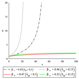
   Figure 12: Plot of the dimensionless Hubble rate $E$ against $x$, for vanishing $\mathcal{D}$, and for an interacting coefficient $\gamma<\frac{1}{2\beta_{\lim}}$. The cosmological parameters are assumed to be $\Omega_{m_{0}}=0.315$, $q_{0}=-0.558$, $\Omega_{\alpha}=0.1$, and $\lambda_{m}=0$. The plot has been done for several values of the holographic parameter, and the interacting parameter $\lambda_{H}$ that are stated at the bottom of the figure.

   Finally, the discriminant $\mathcal{D}$ vanishes when $\beta=\beta_{+}$ or $\beta_{-}$. This can take place on the normal branch for $\gamma<\frac{1}{2\beta_{\lim}}$. The solution of the modified Friedmann equation (41) can be expressed as

   $$E=-\frac{1}{4\Omega_{\alpha}\sqrt{\Omega_{r_{c}}}}\left[(2\gamma\beta-1)-\frac{1}{\mathcal{C}_{3}+\frac{1}{2\gamma\beta}(x-x_{3})}\right],$$ (58)

   where

   $$\mathcal{C}_{3}=\frac{1}{2\gamma\beta-1+4\Omega_{\alpha}\sqrt{\Omega_{r_{c}}}E_{3}},$$ (59)

   $x_{3}$ and $E_{3}$ are integration constants. By taking the limit $x\rightarrow\infty$, the dimensionless Hubble rate (58) reduces to

   $$E_{+}=\frac{(2\gamma\beta-1)}{4\Omega_{\alpha}\sqrt{\Omega_{r_{c}}}},$$ (60)

   $E_{+}$ coincides with the one of Eq. (55) for a vanishing $\mathcal{D}$. The brane can be asymptotically de Sitter for the normal branch if $\frac{1}{2\beta}<\gamma<\frac{1}{2\beta_{\lim}}$, otherwise the Hubble rate $E_{+}$ is negative and the asymptotic analysis performed is no longer valid. This behavior can be seen from the numerical analysis presented in Fig. 12 and the brane undergoes a big freeze singularity with an expansion given by Eq. (56).

   The results of the model for $Q=\lambda_{\mathrm{H}}H\rho_{\mathrm{H}}+\lambda_{\mathrm{m}}H\rho_{\mathrm{m}}$ are similar to those with $Q=\lambda_{\mathrm{H}}H\rho_{\mathrm{H}}$ after making the transformation $\lambda_{H}$ $\longrightarrow\frac{3\lambda_{H}}{3-\lambda_{m}}$ in the model $Q=\lambda_{\mathrm{H}}H\rho_{\mathrm{H}}$.

   

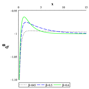
   Figure 13: Plot of the effective equation of state $\omega_{eff}$ against $x$, for $\gamma=\frac{1}{2\beta_{\lim}}$. The cosmological parameters are assumed to be $\Omega_{m_{0}}=0.315$, $q_{0}=-0.558$, $\Omega_{\alpha}=0.1$. The plot has been done for several values of the holographic parameter that are stated at the bottom of the figure.

   

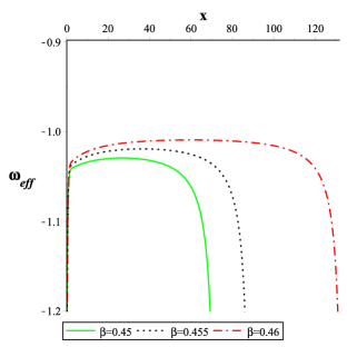
   Figure 14: Plot of the effective equation of state $\omega_{eff}$ against $x$, for the negative sign of $\mathcal{D}$, which correspond to $\gamma<\frac{1}{2\beta_{\lim}}$. The cosmological parameters are assumed to be $\Omega_{m_{0}}=0.315$, $q_{0}=-0.558$, $\Omega_{\alpha}=0.1$, $\lambda_{m}=0$ and $\lambda_{H}=0.3$. The plot has been done for several values of the holographic parameter that are stated at the bottom of the figure.

   

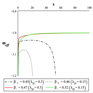
   Figure 15: Plot of the effective equation of state $\omega_{eff}$ against $x$, for the vanishing $\mathcal{D}$. The cosmological parameters are assumed to be $\Omega_{m_{0}}=0.315$, $q_{0}=-0.558$, $\Omega_{\alpha}=0.1$, $\lambda_{m}=0$. The plot has been done for several values of the holographic parameter that are stated at the bottom of the figure.

   

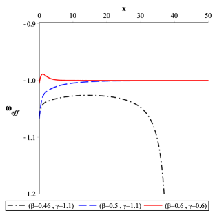
   Figure 16: Plot of the effective equation of state $\omega_{eff}$ against $x$, for the positive sign of $\mathcal{D}$. The cosmological parameters are assumed to be $\Omega_{m_{0}}=0.315$, $q_{0}=-0.558$, $\Omega_{\alpha}=0.1$, $\lambda_{m}=0$. The plot has been done for several values of the holographic parameter, and the interacting parameter $\lambda_{H}$ that are stated at the bottom of the figure.

IV.3 Numerical analysis

The asymptotical analysis we have carried out in the previous subsection can be completed with a numerical analysis of Eq. (II).

Fig. 8 shows some numerical solutions for $\gamma=\frac{1}{2\beta_{\lim}}$ corresponding to the normal branch in which we are interested. As we notice, the brane is asymptotically de Sitter in the future, and the dimensionless Hubble rate $E$ approaches the value $E_{+}=\frac{(\frac{\beta}{\beta_{\lim}}-1)-\sqrt{\mathcal{D}}}{4\Omega_{\alpha}\sqrt{\Omega_{r_{c}}}}.$ For $\gamma\neq\frac{1}{2\beta_{\lim}}$, we discuss the numerical analysis with respect to the sign of the discriminant $\mathcal{D}$: (i) Fig. 9 shows the numerical solutions of Eq. (II) for a negative value of $\mathcal{D}$. The brane expands with respect to $x$ in the future until it reaches a big freeze singularity which is consistent with our analytical results, (ii) For a positive sign of $\mathcal{D}$ and for $\gamma<\frac{1}{2\beta_{\lim}}$, Fig. 10 shows that the brane expands until it reaches a big freeze singularity for $\beta=0.45$, and $\beta=0.52$ for $\gamma<\frac{1}{2\beta}$, and a de Sitter solution for $\beta=1/2$ and $\beta=0.6$, for $\gamma>\frac{1}{2\beta}$. These results are similar to our previous analytical analysis. For $\gamma>\frac{1}{2\beta_{\lim}}$ the numerical solutions behave like a de Sitter solutions as shown in Fig. 11, which is of course consistent with the analytical results, (iii) When the discriminant $\mathcal{D}$ vanishes, the solutions are shown in Fig 12. The brane expands with respect to $x$ in the future until it reaches a big freeze for $\beta=0.45$, and $\beta=0.46$ for $\gamma<\frac{1}{2\beta}$, and behaves like a de Sitter solution for $\beta=0.47$, and $\beta=0.51$ for $\gamma>\frac{1}{2\beta}$. All of these solutions again are consistent with our previous analytical analysis.

For completeness, we plot in Figs. 13-16 the behaviours of the effective equation of state, $\omega_{eff}$, defined in Eq. (38)-(39) where $\rho_{\text{eff}}$ reads in this case

$$\rho_{\text{eff}}=3M_{p}^{2}H_{0}^{2}\Big{[}\frac{1}{2}\beta\frac{dE^{2}}{dx}+2\beta E^{2}-2\sqrt{\Omega_{\mathrm{r_{c}}}}(1+\Omega_{\mathrm{\alpha}}E^{2})E\Big{]}$$ (61)

Fig. 13 shows the behaviours of the effective equation of state for $\gamma=\frac{1}{2\beta_{\textrm{lim}}}$. At the far future $\omega_{eff}$ has a phantom like even though the brane follows a de sitter behaviour.

Fig. 14 shows the behaviours of the effective equation of state for the negative sign of $\mathcal{D}$ i.e. $\gamma<\frac{1}{2\beta_{\textrm{lim}}}$. The parameter $\omega_{eff}$ has a phantom like behaviour and the brane ends its expansion in a big freeze singularity.

Fig. 15 shows the behaviours of the effective equation of state for the vanishing $\mathcal{D}$. Once again the parameter $\omega_{eff}$ has a phantom like for $\frac{1}{2\beta}<\gamma<\frac{1}{2\beta_{\textrm{lim}}}$ even though the brane follows a de sitter expansion while for $\gamma<\frac{1}{2\beta}<\frac{1}{2\beta_{\textrm{lim}}}$ the brane ends its behaviours in a big freeze singularity.

Fig. 16 shows the behaviours of the effective equation of state for a positive sign of $\mathcal{D}$. The equation of state parameter $\omega_{eff}$ has a phantom like behaviour with two possible end states of the brane: (i) A de sitter behaviour of the brane for $\frac{1}{2\beta_{\textrm{lim}}}<\gamma$ e.g. $\beta=0.6$ and $\gamma=0.6$ and for $\frac{1}{2\beta}<\gamma<\frac{1}{2\beta_{\textrm{lim}}}$ e.g. $\beta=0.5$ and $\gamma=1.1$ (ii) while for $\gamma<\frac{1}{2\beta_{\textrm{lim}}}$ the brane ends its behaviours in a big freeze singularity.

			Without a Gauss-Bonnet term
Sec.	Interacting model	$\lambda$	$\beta$		Late time behaviour
III A	$\lambda_{\rm m}\neq 0,\lambda_{\rm H}=0$	$\lambda_{\rm m}=3$	$-$		Non physical
		$\lambda_{\rm m}\neq 3$	$\beta=\frac{1}{2}$		LR
		$\lambda_{\rm m}\neq 3$	$\beta>\frac{1}{2}$		de Sitter
		$\lambda_{\rm m}\neq 3$	$\beta_{lim}<\beta<\frac{1}{2}$		BR
III B	$\lambda_{\rm m}=0,\lambda_{\rm H}\neq 0$	-$-$	$\beta=\beta_{LR}=\frac{3}{2(\lambda_{\rm H}+3)}$		LR
			$\beta<\beta_{LR}$		BR
			$\beta>\beta_{LR}$		de Sitter
III C	$\lambda_{\rm m}\neq 0,\lambda_{\rm H}\neq 0$	$\lambda_{\rm m}=3$	$-$		Minkowski
		$\lambda_{\rm H}=\lambda_{\rm m}-3$	$-$		Non physical
		$\lambda_{\rm H}\neq\lambda_{\rm m}-3$	$\beta=\beta_{LR}=\frac{3-\lambda_{\rm m}}{2(\lambda_{\rm H}-2(\lambda_{\rm m}+6)}$		LR
			$\beta>\beta_{LR}$		de Sitter
			$\beta<\beta_{LR}$		BR
			With a Gauss-Bonnet term
Sec.	Interacting model	${\cal{D}}$	$\gamma$	$\lambda$	Late time behaviour
IV A	$\lambda_{\rm m}\neq 0,\lambda_{\rm H}=0$	$-$	$1$	$\lambda_{\rm m}=3$	Non physical
		$-$	$1$	$\lambda_{\rm m}\neq 3$	Big Freeze OualiPRD85
IV B ∗	$\lambda_{\rm m}=0,\lambda_{\rm H}\neq 0$	${\cal{D}}<0$	$\gamma<\frac{1}{2\beta_{lim}}$	$-$	Big Freeze
		$0\leq{\cal{D}}$	$\frac{1}{2\beta}<\gamma\leq\frac{1}{2\beta_{lim}}$	$-$	de Sitter
			$\gamma<\frac{1}{2\beta}<\frac{1}{2\beta_{lim}}$	$-$	Big Freeze

Table 1: Summary of the behaviours of the universe at late time, for different DM and DE interactions. (^∗) The case $\lambda_{\rm m}\neq 0,\lambda_{\rm H}\neq 0$ is obtained by replacing $\lambda_{\rm H}$ by $\frac{3\lambda_{\rm H}}{3-\lambda_{\rm m}}$ in the expressions of $\gamma$ and ${\cal{D}}$.

V Conclusions

In this paper, we have presented an interacting holographic Ricci dark energy model (IHRDE) with a cold dark matter (CDM) component in an induced gravity brane world model. We have shown that the late time acceleration of the universe is consistent with the current observational data with and without a Gauss-Bonnet (GB) curvature term in the bulk action.

The parameter $\beta$ that characterizes HRDE is very important in determining the asymptotic behaviour of the holographic Ricci dark energy (HRDE) and that of the brane. The parameter $\beta$ is bounded by a limiting value, $\beta_{\textrm{lim}}$, that splits the self-accelerating branch from the normal one. In this paper, we have considered only the normal branch, i.e. $\beta>\beta_{\textrm{lim}}$, which suffers from the big rip and the little rip singularities (see Ref. OualiPRD85 ). Assuming that, at present, our model does not deviate too much from $\Lambda$CDM, the value of $\beta_{\textrm{lim}}$ is estimated to be of the order $0.44$.

The interaction is characterized by the quantity $Q=\lambda_{H}H\rho_{H}+\lambda_{m}H\rho_{m}$ where $\lambda_{H}$ and $\lambda_{m}$ are the coupling characterizing the HRDE and the CDM interaction.

For a vanishing $\lambda_{H}$, the interaction model characterized only by the CDM energy does not succeed to remove the big freeze singularity occurring in the non interacting model OualiPRD85 with and without the GB curvature term.

For a vanishing $\lambda_{m}$, the model with interaction between the dark sector of the universe can be splited into two cases:

• Without a GB term the IHRDE model shows that the interaction removes the little rip singularity for $\beta=1/2$ to $\beta=\frac{3}{2(3+\lambda_{H})}$, and reduces the width of the big rip singularity from $\beta_{\textrm{lim}}<\beta<1/2$ to $\beta_{\textrm{lim}}<\beta<\frac{3}{2(3+\lambda_{H})}<1/2$. Therefore an appropriate choice of the coupling $\lambda_{H}$ such that $\frac{3}{2(3+\lambda_{H})}<\beta_{lim}$ avoids the big rip and the little rip and hence the IHRDE gives a satisfactory and an alternative description of the late time cosmic acceleration of the universe as compared to the HRDE. Indeed the later one modifies the big rip and little rip into a big freeze one while the former removes them definitively. Furthermore the IHRDE will have a phantom-like behaviour even though the brane undergoes a de Sitter stage at the very late time.
  

• With a GB term in the bulk the IHRDE model depends on the sign of the discriminant ${\mathcal{D}}$ through the parameter $\beta$, the GB parameter, and the coupling $\gamma$. In the particular case $\gamma=\frac{1}{2\beta_{\textrm{lim}}}$, the interacting model succeed in removing the big rip and little rip singularity from the brane future evolution and it will evolve asymptotically as a de Sitter universe as is shown in Fig. 13. For $\gamma\neq\frac{1}{2\beta_{\textrm{lim}}}$, the situation depends on the sign of the discriminant ${\mathcal{D}}$:

  1. If ${\mathcal{D<}}0$, which correspond to $\gamma<\frac{1}{2\beta_{\lim}}$. The brane expand in the future until it reaches a big freeze singularity as is shown in Fig. 14.

  2. If ${\mathcal{D}}=0$, two situations can be found (as is shown in Fig. 15)

     a-

     When $\frac{1}{2\beta}<\gamma<\frac{1}{2\beta_{\textrm{lim}}}$, the brane is asymptotically de Sitter.

     b-

     When $\gamma<\frac{1}{2\beta}<\frac{1}{2\beta_{\textrm{lim}}}$, the brane hits a big freeze singularity.

  3. If ${\mathcal{D}}>0$, two situations can be found (as is shown in Fig. 16)

     a-

     When $\gamma>\frac{1}{2\beta_{\textrm{lim}}},$ the brane expands in the future until it reaches a de Sitter stage.

     b-

     When $\gamma<\frac{1}{2\beta_{\textrm{lim}}},$ the brane becomes asymptotically de Sitter in the future for $\gamma>\frac{1}{2\beta}$, while for $\gamma<\frac{1}{2\beta}$ the brane hits a big freeze singularity.

Taking into account both couplings $\lambda_{m}$ and $\lambda_{H}$ the description of the interaction between CDM and HRDE is similar to the interaction characterised only by $\lambda_{H}$ in the HRDE by replacing the coupling $\lambda_{H}$ in the interaction form $Q=\lambda_{H}H\rho_{H}$ by the quantity $\frac{3\lambda_{H}}{3-\lambda_{m}}$. The same conclusions are obtained by requiring that the constraints on the parameter $\gamma$ are verified for the sets of the couple $(\lambda_{m},\lambda_{H})$ for which $\gamma=1+\frac{\lambda_{H}}{3-\lambda_{m}}$.

- (1) S. Perlmutter et al., Astrophys. J. 517, 565 (1999) [arXiv:astro-ph/9812133]; A. G. Riess et al., Astron. J. 116, 1009 (1998) [arXiv:astro-ph/9805201]. M. Kowalski et al., Astrophys. J. 686, 749 (2008) [arXiv:0804.4142].
- (2) D. N. Spergel et al., Astrophys. J. Suppl. 148, 175 (2003) [arXiv:astro-ph/0302209]; ibid. Astrophys. J. Suppl. 170, 377 (2007) [arXiv:astro-ph/0603449]; E. Komatsu et al. [WMAP Collaboration], Astrophys. J. Suppl. 180, 330 (2009) [arXiv:0803.0547].
- (3) M. Tegmark, et al., SDSS Collaboration, Phys. Rev. D 69, 103501 (2004) [arXiv:astro-ph/0310723]; J.K. Adelman-McCarthy, et al., SDSS Collaboration, Astrophys. J. Suppl. 175, 297 (2008) , [arXiv:0707.3413].
- (4) N. Aghanim et al. [Planck Collaboration], [arXiv:1807.06209].
- (5) P.J.E. Peebles and B. Ratra, Rev. Mod. Phys. 75, 559 (2003) [astro-ph/0207347].
- (6) B. Ratra and P.J.E. Peebles, Phys. Rev. D 37, 3406 (1988); I. Zlatev, L. Wang and P.J. Steinhardt, Phys. Rev. Lett. 82, 896 (1999).
- (7) Armendariz-Picon , Essentials of K-essence, Phys. Rev. D 63, 103510 (2001).
- (8) R.R. Caldwell, Phys. Lett. B 545, 23 (2002); S.M. Carroll, M. Hoffman and M. Trodden, Phys. Rev. D 68, 023509 (2003); J. G. Hao, X. Z. Li, Phys. Rev. D 68, 043501 (2003); D. J. Liu, X. Z. Li, Phys. Rev. D 68, 067301 (2003).
- (9) S. í. Nojiri, S. D. Odintsov and S. Tsujikawa, Phys. Rev. D 71, 063004 (2005) [arXiv:0501025]
- (10) J. D. Barrow, Class. Quant. Grav. 21, L79 (2004); J. D. Barrow and C. G. Tsagas, Class. Quant. Grav. 22, 1563 (2005); V. Gorini, A. Y. .Kamenshchik, U. Moschella and V. Pasquier, Phys. Rev. D 69, 123512 (2004).
- (11) M. Bouhmadi-López, P. F. Gonzalez-Díaz and P. Martín-Moruno, Phys. Lett. B 659, 1 (2008) [gr-qc/0612135].
- (12) L. P. Chimento and M. G. Richarte, Phys. Rev. D 93, 043524 (2016) [arXiv:1512.02664 [gr-qc]].
- (13) M. Cataldo, L. P. Chimento and M. G. Richarte, Phys. Rev. D 95, 063510 (2017) [arXiv:1702.07743].
- (14) T. Ruzmaikina and A. A. Ruzmaikin, Sov. Phys. JETP 30, 372 (1970).
- (15) S. í. Nojiri and S. D. Odintsov, Phys. Rev. D 72, 023003 (2005) [hep-th/0505215].
- (16) H. Stefancić, Phys. Rev. D 71, 084024 (2005) [astro-ph/0411630].
- (17) M. Bouhmadi-López, Nucl. Phys. B 797, 78 (2008) [astro-ph/0512124].
- (18) P. H. Frampton, K. J. Ludwick, and R. J. Scherrer, Phys. Rev. D 84, 063003 (2011) [arXiv:1106.4996].
- (19) I. Brevik, E. Elizalde, S. í. Nojiri, and S. D. Odintsov, Phys. Rev. D 84, 103508 (2011) [arXiv:1107.4642].
- (20) M. Bouhmadi-López, P. Chen, and Y. W. Liu, Eur. Phys. J. C 73, 2546 (2013) [arXiv:1302.6249].
- (21) M. Bouhmadi-López, A. Errahmani, P. Martín-Moruno, T. Ouali and Y. Tavakoli, Int. J. Mod. Phys. D 24, 1550078 (2015) [arXiv:1407.2446].
- (22) M. Bouhmadi-López, A. Errahmani, T. Ouali and Y. Tavakoli, Eur. Phys. J. C 78, 330 (2018) [arXiv:1707.07200].
- (23) G. ’t Hooft, [arXiv:gr-qc/9310026].
- (24) L. Susskind, J. Math. Phys. 36, 6377 (1995) [arXiv:hep-th/9409089].
- (25) J. D. Bekenstein, Phys. Rev. D 7, 2333 (1973); J. D. Bekenstein, Phys. Rev. D 9, 3292 (1974); J. D. Bekenstein, Phys. Rev. D 23, 287 (1981); J. D. Bekenstein, Phys. Rev. D 49, 1912 (1994); S. W. Hawking, Commun. Math. Phys. 43, 199 (1975); S. W. Hawking, Phys. Rev. D 13, 191 (1976).
- (26) A. G. Cohen, D. B. Kaplan and A. E. Nelson, Phys. Rev. Lett. 82, 4971 (1999) [arXiv:hep-th/9803132].
- (27) M. Li, Phys. Lett. B 603, 1 (2004) [arXiv:hep-th/0403127].
- (28) S. D. H. Hsu, Phys. Lett. B 594, 13 (2004) [arXiv:hep-th/0403052].
- (29) O. Luongo, L. Bonanno, G. Iannone, Int. Jour. Mod. Phys. D, 21, 12, 1250091 (2012); A. Aviles, L. Bonanno, O. Luongo, H. Quevedo, Phys. Rev. D 84, 103520, (2011).
- (30) C. Gao, F.Q. Wu, X. Chen, Y.G. Shen, Phys. Rev. D 79, 043511 (2009) [arXiv: 0712.1394].
- (31) S. í. Nojiri and S. D. Odintsov, Gen. Relativ. Gravit. 38, 1285 (2006).
- (32) M. H. Belkacemi, M. Bouhmadi-López, A. Errahmani, and T. Ouali, Phys. Rev. D 85, 083503 (2012).
- (33) G. R. Dvali, G. Gabadadze, M. Porrati, Phys. Lett. B484, 112-118 (2000). [hep-th/0002190]; ibid. Phys. Lett. B485, 208-214 (2000). [hep-th/0005016].
- (34) C. Deffayet, Phys. Lett. B 502, 199 (2001) [arXiv:hep-th/0010186].
- (35) V. Sahni and Y. Shtanov, J. Cosmol. Astropart. Phys. 11, 014 (2003); L. P. Chimento, R. Lazkoz, R. Maartens, and I. Quiros, J. Cosmol. Astropart. Phys. 09, 004 (2006).
- (36) H. S. Zhang and Z. H. Zhu, Phys. Rev. D 75, 023510 (2007); M. Bouhmadi-López and R. Lazkoz, Phys. Lett. B 654, 51 (2007).
- (37) M. Bouhmadi-López, JCAP 0911, 011 (2009) [arXiv:0905.1962]; M. Bouhmadi-López, S. Capozziello, V. F. Cardone, Phys. Rev. D82, 103526 (2010) [arXiv:1010.1547]; M. Li, Phys. Lett. B 603, 1 (2004).
- (38) Abdul Jawad, Shamaila Rani, Ines G. Salako, Faiza Gulshan, Eur. Phys. J. Plus 131, 236 (2016) [arXiv:1608.01181].
- (39) Jibitesh Dutta, Wompherdeiki Khyllep, Erickson Syiemlieh, Eur. Phys. J. Plus 131, 33 (2016) [arXiv:1602.03329].
- (40) A. Ravanpak, H. Farajollahi, G. F. Fadakar, Res. Astron. Astrophys. 16, 137 (2016) [arXiv:1610.09614].
- (41) H. Farajollahi, A. Ravanpak, G. F. Fadakar, Astrophys. Space Sci. 348, 253 (2013) [arXiv:1606.00845].
- (42) A. Sheykhi, M. H. Dehghani, S. Ghaffari, Int. J. Mod. Phys. D 25, 1650018 (2016) [arXiv:1506.02505].
- (43) S. Ghaffari, M. H. Dehghani, A. Sheykhi, Phys. Rev. D 89, 123009 (2014) [arXiv:1506.01676].
- (44) Y. Shtanov and V. Sahni, Class. Quant. Grav. 19, L101 (2002) [gr-qc/0204040].
- (45) L. Amendola, Phys. Rev. D 62, 043511 (2000); L. Amendola and C. Quercellini, Phys. Rev. D 68, 023514 (2003); L. Amendola, S. Tsujikawa and M. Sami, Phys. Lett. B 632, 155 (2006).
- (46) M. Bouhmadi-López, J. Morais and A. Zhuk, Phys. Dark Univ. 14, 11 (2016) [arXiv:1603.06983].
- (47) J. Morais, M. Bouhmadi-López, K. Sravan Kumar, J. Marto and Y. Tavakoli, Phys. Dark Univ. 15, 7 (2017) [arXiv:1608.01679].
- (48) C. G. Boehmer, G. Caldera-Cabral, R. Lazkoz, R. Maartens, Phys. Rev. D 78, 023505 (2008).
- (49) S. B. Chen, B. Wang, J. L. Jing, Phys. Rev.D 78, 123503 (2008).
- (50) D. Pavón,W. Zimdahl, Phys. Lett. B 628, 206 (2005).
- (51) S. Campo, R. Herrera, D. Pavón, Phys. Rev. D 78, 021302 (2008).
- (52) I. Duran, D. Pavon, Phys. Rev. D 83, 023504 (2011) [arXiv:1012.2986].
- (53) E. G. M. Ferreira, J. Quintin, A. A. Costa, E. Abdalla and B. Wang, Phys. Rev. D 95, no. 4, 043520 (2017) [arXiv:1412.2777].
- (54) T. Delubac et al. [BOSS Collaboration], Astron. Astrophys. 574 (2015), A59 [arXiv:1404.1801].
- (55) A. Sheykhi, M. H. Dehghani, S. Ghaffari, Int. J. Mod. Phys. D, 25, 1650018 (2016) [arXiv:1506.02505].
- (56) B. Wang, Y. Gong, E. Abdalla, Phys. Lett. B 624, 141 (2005).
- (57) L. P. Chimento and M. G. Richarte, Phys. Rev. D 86, 103501 (2012) [arXiv:1210.5505].
- (58) L. P. Chimento, M. Forte and M. G. Richarte, Eur. Phys. J. C 73, 2285 (2013) [arXiv:1301.2737].
- (59) M. Bouhmadi-López, A. Errahmani, and T. Ouali, Phys. Rev. D 84, 083508 (2011).
- (60) Z. K. Guo, N. Ohta, S. Tsujikawa, Phys. Rev. D 76, 023508 (2007).
- (61) G. Olivares, F. Atrio-Barandela and D. Pavón, Phys. Rev. D 74, 043521 (2006), J.H. He, B. Wang, JCAP 06, 010 (2008).
- (62) B. Wang, E. Abdalla, F. Atrio-Barandela and D. Pavon, Rept. Prog. Phys. 79, 096901 (2016) [arXiv:1603.08299].
- (63) B. Wang, C.-Y. Lin, D. Pavon, E. Abdalla, Phys. Lett. B 662, 1 (2008).
- (64) D. Pavón, Bin Wang, Gen. Rel. Grav. 41, 1 (2009).
- (65) B. Wang, C.-Y. Lin, E. Abdalla, Phys. Lett. B 637, 357 (2006).
- (66) S. Campo, R. Herrera, G. Olivares, D. Pavón, Phys. Rev. D 74, 023501 (2006).
- (67) S. Campo, R. Herrera, D. Pavón, Phys. Rev. D 71, 123529 (2005).
- (68) J. H. He, B. Wang and E. Abdalla, Phys. Lett. B 671, 139 (2009) [arXiv:0807.3471].
- (69) J. H. He, B. Wang and E. Abdalla, Phys. Rev. D 83, 063515 (2011) [arXiv:1012.3904].
- (70) C. Feng, B. Wang, E. Abdalla and R. K. Su, Phys. Lett. B 665, 111 (2008) [arXiv:0804.0110].
- (71) G. Kofinas, R. Maartens and E. Papantonopoulos, JHEP 0310, 066 (2003) [arXiv:hep-th/0307138].
- (72) M. Bouhmadi-López and P. V. Moniz, Phys. Rev. D 78, 084019 (2008) [arXiv:0804.4484]; M. Bouhmadi-López, Y. Tavakoli and P. V. Moniz, JCAP 1004, 016 (2010) [arXiv:0911.1428].
- (73) R. A. Brown, R. Maartens, E. Papantonopoulos and V. Zamarias, JCAP 0511, 008 (2005) [arXiv:gr-qc/0508116]; R. A. Brown, Gen. Rel. Grav. 39, 477 (2007) [arXiv:0602050]; R. G. Cai, H. S. Zhang and A. Wang, Commun. Theor. Phys. 44, 948 (2005) [arXiv:0505186].
- (74) M. Bouhmadi-López, P. F. González-Díaz, and P. Martín- Moruno, Phys. Lett. B 659, 1 (2008); ibid, Int. J. Mod. Phys. D 17, 2269 (2008).