Magneto-Electric Response of Quantum Structures Driven by Optical Vector Beams

Abstract

Key advances in the generation and shaping of spatially structured photonic fields both in the near and far field render possible the control of the duration, the phase, and the polarization state of the field distributions. For instance, optical vortices having a structured phase are nowadays routinely generated and exploited for a range of applications. While the light-matter interaction with optical vortices is meanwhile well studied, the distinctive features of the interaction of quantum matter with vector beams, meaning fields with spatially inhomogeneous polarization states, are still to be explored in full detail, which is done here. We analyze the response of atomic and low dimensional quantum structures to irradiation with radially or azimuthally polarized cylindrical vector beams. Striking differences to vortex beams are found: Radially polarized vector beams drive radially breathing charge-density oscillations via electric-type quantum transitions. Azimuthally polarized vector beams do not affect the charge at all but trigger, via a magnetic vector potential a dynamic Aharonov–Bohm effect, meaning a vector-potential driven oscillating magnetic moment. In contrast to vortex beams, no unidirectional currents are generated. Atoms driven by a radially polarized vector beam exhibit angular momentum conserving quadrupole transitions tunable by a static magnetic field, while when excited with azimuthally polarized beam different final-state magnetic sublevels can be accessed.

I Introduction

Spatio-temporally modulated electromagnetic (EM) fields in general, and laser fields in particular, have been the driving force for numerous discovery in science as in femto-chemistry and attosecond physics both relying on the controlled temporal shaping of laser fields Brabec and Krausz (2000); Petek and Ogawa (1997). Spatially structured EM fields, which are in the focus of research currently, have also proved instrumental for a wide range of applications such as particle trapping Ng et al. (2010), high-resolution lithography Hao et al. (2010); Dorn et al. (2003); Kang et al. (2012); Bauer et al. (2014), quantum memories Parigi et al. (2015), optical communication Dámbrosio et al. (2012); Vallone et al. (2014), classical entanglement Gabriel et al. (2011), and as a magnetic nanoprobe for enhancing the near field magnetic component Guclu et al. (2016).

Prominent examples of structured EM fields are orbital-angular momentum carrying (OAM) vortex beams and vector beams (VBs). OAM beams possess an inhomogeneous azimuthal phase distribution and a homogeneous polarization. For VBs the spatial distributions of both the phase and the polarization in the plane perpendicular to the propagation of the EM wave are inhomogeneous. The spatial structuring brings about several advantages. For instance, a radially polarized VB allows for a sharper focusing. It may also have a strong centered longitudinal field Dorn et al. (2003), offering a tool for investigating new aspects of light-matter interaction, as detailed below. On the other hand, an azimuthally polarized VB has a smaller spot size than a radially polarized VB Hao et al. (2010) and interact with quantum matter in fundamentally different manner, as shown here. Phase modulated beams carrying OAM Bliokh et al. (2015) serve further purposes. For instance, such beams were used to study otherwise inaccessible angular momentum state of atoms Schmiegelow et al. (2016) and to generate unidirectional steady-state charge currents in molecular matter or in nanostructures  Wätzel and Berakdar (2016); Wätzel et al. (2016) pointing so to qualitatively new routes in optomagnetism.

Theoretically, key quantities for understanding the fundamental of the interaction of structured fields with matter are the associated EM vector $\boldsymbol{A}(\boldsymbol{r},t)$ and scalar $\Phi(\boldsymbol{r},t)$ potentials that couple, respectively to the sample’s currents and charge densities. Homogeneous optical EM fields irradiating a quantum object (with a charge localization below the EM-field wavelength) induce mainly electric-dipole transitions in the sample and to a much smaller degree magnetic-dipole transitions. At moderate intensities, the ratio of the magnetic dipole to the electric dipole absorption rate is proportional to the ratio of the magnetic to the electric field strengths $\left|\boldsymbol{H}\right|^{2}/\left|\boldsymbol{E}\right|^{2}$ Zurita-Sánchez and Novotny (2002). Therefore, tailored laser beams with engineered magnetic to electric-field ratio may boost the magnetic transitions. For instance, this can be accomplished in the near-field of an object with a small circular aperture Hanewinkel et al. (1997). For the nm apertures experimentally feasible so far, the magnetic transitions enhancement is negligibly small, however Hanewinkel et al. (1997). In this context, cylindrical VBs with azimuthal or radial polarization offer an interesting alternative. For azimuthally polarized VBs the magnetic to electric field ratio is substantial: one can show that $\left|\boldsymbol{H}\right|/\left|\boldsymbol{E}\right|=1/\eta_{0}$ on the beam axis where $\eta_{0}$ is the free-space impedance Veysi et al. (2015); Zurita-Sánchez and Novotny (2002). The VBs we will be dealing with can be experimentally realized by the coherent interference of two TEM₀₁ laser modes which are orthogonally polarized Oron et al. (2000). Other techniques involve interferometry Tidwell et al. (1990), holograms Churin et al. (1993), liquid crystal polarizer Stalder and Schadt (1996), spatial light modulators Tripathi and Toussaint (2012) and multi-elliptical core fibers Giovani Milione, Henry I. Sztul, Dan A. Nolan, Jonathan Kim (2011). Planar fabrication technologies in connection with flat optics devices could also produce cylindrical VBs Memarzadeh and Mosallaei (2011); Yu et al. (2011, 2012). A further approach relies on the conversion of circularly polarized light into radially or azimuthally VBs (in the far-infrared Bomzon et al. (2002) and visible range Beresna et al. (2011)) by space-variant gratings. A method involving an inhomogeneous half-wave plate metasurface to generate VBs was also demonstrated Yi et al. (2014); Liu et al. (2014) where the efficiency was increased when employing suitable metamaterials Veysi et al. (2015).

VBs possess a pronounced longitudinal component that can be employed for Raman-spectroscopy Saito et al. (2008), material-processing Wang et al. (2008); Meier et al. (2007) or tweezers for metallic particles Zhan (2004). For OAM carrying beams, the longitudinal component may serve for studying subband states in a quantum well Sbierski et al. (2013) and hole-states in quantum dots Quinteiro and Kuhn (2014). The various facets of the interactions of VBs with quantum matter will be addressed in this present work. As a demonstration of the formal theory, we will study the nature of bound-bound and bound-continuum transitions caused by VBs when interacting with quantum systems such as nanostructures or atoms. As demonstrated here the interaction of such fields is not only fundamentally different from non-structured fields but also, radial VBs interact with matter in a qualitatively different way as azimuthal VBs do, and the employment of both offer qualitatively new opportunities for accessing the magneto-electric response of quantum matter at moderate intensities.

II Light-Matter Interaction with Cylindrical Vector Beams

A cylindrical vector beam may be composed from two counter-rotating circularly polarized optical vortex beams. The most prominent feature of such a vortex EM beam is the azimuthal phase structure described by $\exp(\mathrm{i}m_{\rm OAM}\varphi)$ where $\varphi$ is the azimuthal angle in the $xy$ plane Allen et al. (1992); Yao and Padgett (2011), transverse to the propagation direction (which sets the $z$-direction, the radial distance we denote by $\rho$). The parameter $m_{\rm OAM}$ is the vortex topological charge that determines the amount of the carried orbital angular momentum (OAM), and can potentially be transferred to a sample Quinteiro et al. (2011); Quinteiro and Kuhn (2014); Wätzel and Berakdar (2016). The wave vector along $z$ is $q_{\parallel}$. Optical vortices have a phase singularity at $\rho=0$ and thus a vanishing intensity at this point. Generally, the transverse spatial distribution is characterized by the function $f_{m_{\rm OAM}}(\rho)$ which can be of a Laguerre–Gaussian type Allen et al. (1992), Hermite–Gaussian Novotny et al. (1998) type or Bessel type Garces-Chavez et al. (2002) with the main difference being the radial intensity localization. For nano-scale objects centered in the vicinity of the optical axis, the different radial distributions of diffraction limited vortex beams have similar influence (due to the vast difference between electronic and optical wave lengths). The change in this behavior with increasing ${\rm OAM}$ can be inferred from the fact that $f_{m_{\rm OAM}}(\rho)\sim\rho^{\left|m_{\rm OAM}\right|}$ for $\rho\rightarrow 0$. As an example, we concentrate on Bessel beams which are exact solution of the Helmholtz equation Garces-Chavez et al. (2002), meaning that our theoretical considerations are beyond the paraxial approximation. Bessel beams are non-diffracting beam solutions with the radial profiles being independent of the propagation direction $z$ and the associated electromagnetic vector potential is a solenoidal vector field: $\nabla\cdot\boldsymbol{A}(\boldsymbol{r},t)\equiv 0$. For the electromagnetic field components follows ($\boldsymbol{r}=\left\{\rho,\varphi,z\right\}$ and $\Re$ means real part)

$$\boldsymbol{A}(\boldsymbol{r},t)=\Re\left\{\mathrm{e}^{\mathrm{i}(q_{\parallel}z-\omega t)}\left[\hat{e}_{\sigma}J_{m_{\rm OAM}}(q_{\perp}\rho)\mathrm{e}^{\mathrm{i}m_{\rm OAM}\varphi}\vphantom{\frac{q_{\perp}}{q_{\parallel}}}-\mathrm{i}\sigma\hat{e}_{z}\frac{q_{\perp}}{q_{\parallel}}J_{m_{\rm OAM}+\sigma}(q_{\perp}\rho)\mathrm{e}^{\mathrm{i}(m_{\rm OAM}+\sigma)\varphi}\right]\right\}$$ (1)

where $A_{0}$ is the vector potential amplitude and $\omega$ is the light frequency. The longitudinal and radial wave vectors satisfy the relation $q_{\parallel}^{2}+q_{\perp}^{2}=(\omega/c)^{2}$. The functions $J_{n}(x)$ are the Bessel functions of $n$th order while the polarization state is characterized by $\hat{e}_{\sigma}=\mathrm{e}^{\mathrm{i}\sigma\varphi}\left(\hat{e}_{\rho}+\mathrm{i}\sigma\hat{e}_{\varphi}\right)$, with $\sigma=\pm 1$. The ratio $q_{\perp}/q_{\parallel}=:\tan\alpha$. Consequently, the angle $\alpha$ characterizes the spatial extent of the intensity profile. A large transverse wave vector means a tighter focusing. Since Bessel beams satisfy also the Coulomb gauge, the electric field reads $\boldsymbol{E}(\boldsymbol{r},t)=-\partial_{t}\boldsymbol{A}(\boldsymbol{r},t)$ while the magnetic field is given by $\boldsymbol{B}(\boldsymbol{r},t)=\boldsymbol{\nabla}\times\boldsymbol{A}(\boldsymbol{r},t)$.

An azimuthally polarized cylindrical VB (we refer to as AVB) can be expressed as a linear combination of two optical vortices with $\{m_{\rm OAM}=+1,\sigma=-1\}$ and $\{m_{\rm OAM}=-1,\sigma=+1\}$, namely

$$\boldsymbol{A}_{\rm AVB}(\boldsymbol{r},t)=A_{0}J_{1}(q_{\perp}\rho)\sin(q_{\parallel}z-\omega t)\hat{e}_{\varphi}.$$ (2)

A radially polarized cylindrical VB (denoted by RVB) is expressible as the difference of the two optical vortices

$$\boldsymbol{A}_{\rm RVB}(\boldsymbol{r},t)=A_{0}\left[-J_{1}(q_{\perp}\rho)\cos(q_{\parallel}z-\omega t)\hat{e}_{\rho}\vphantom{\frac{q_{\perp}}{q_{\parallel}}}+\frac{q_{\perp}}{q_{\parallel}}J_{0}(q_{\perp}\rho)\sin(q_{\parallel}z-\omega t)\hat{e}_{z}\right].$$ (3)

A hallmark of AVB and RVB is the vanishing of the azimuthal-plane component of the field at $\rho=0$. Moreover, AVB and RVB possess a non-vanishing longitudinal component: beams with the azimuthal polarization have a magnetic component at the origin while the longitudinal component of the radially polarized light mode (RVB) is electric. The explicit electric and magnetic fields for both vector beam classes can be found in the first section of the Supporting Information (SI).

We find that for both VBs the minimal coupling to matter is still viable leading to the general interaction operator $\hat{H}_{\rm int}$ with a collection of charge carriers with effective mass $m_{e}^{*}$ and charge $-e$

$$\begin{split}\hat{H}_{\rm int,tot}&=\sum_{i}\hat{H}_{\rm int,i},\\ \hat{H}_{\rm int,i}&=-\frac{e}{2m_{e}^{*}}\left[\hat{\boldsymbol{p}_{i}}\cdot\boldsymbol{A}(\boldsymbol{r}_{i},t)+\boldsymbol{A}(\boldsymbol{r}_{i},t)\cdot\hat{\boldsymbol{p}_{i}}\right]+e\Phi(\boldsymbol{r}_{i},t)\end{split}$$ (4)

$\hat{\boldsymbol{p}_{i}}$ is the linear momentum operator of particle $i$ at the position $\boldsymbol{r}_{i}$ (for moderate intensities we may suppress the term $\boldsymbol{A}^{2}(\boldsymbol{r}_{i},t)$). It is instructive to exploit the gauge invariance of observables and go over to the potentials (for brevity index $i$ is suppressed)

$$\boldsymbol{A}^{\prime}(\boldsymbol{r},t)=-\boldsymbol{r}\times\int_{0}^{1}\mathrm{d}\lambda\,\lambda\boldsymbol{B}(\lambda\boldsymbol{r},t)$$ (5)

and

$$\Phi^{\prime}(\boldsymbol{r},t)=-\boldsymbol{r}\cdot\int_{0}^{1}\mathrm{d}\lambda\,\boldsymbol{E}(\lambda\boldsymbol{r},t)$$ (6)

The choice is referred to the Poincaré gauge or generally the multipole gauge Cohen-Tannoudji et al. (1989, 1992). Note that in this gauge $\boldsymbol{r}\cdot\boldsymbol{A}^{\prime}(\boldsymbol{r},t)\equiv 0$ and $\boldsymbol{B}(\boldsymbol{r},t)=\boldsymbol{\nabla}\times\boldsymbol{A}^{\prime}(\boldsymbol{r},t)$ while $\boldsymbol{E}(\boldsymbol{r},t)=-\partial_{t}\boldsymbol{A}^{\prime}(\boldsymbol{r},t)-\boldsymbol{\nabla}\Phi^{\prime}(\boldsymbol{r},t)$. With eqs (5) and (6), the light-matter interaction can be expressed as a sum of a pure electric and magnetic contributions $\hat{H}_{\rm int}=\hat{H}_{\rm el}+\hat{H}_{\rm magn}$, where

$$\hat{H}_{\rm el}(t)=e\Phi^{\prime}(\boldsymbol{r},t)=e\,\boldsymbol{r}\cdot\boldsymbol{E}^{\prime}(\boldsymbol{r},t)$$ (7)

and $\boldsymbol{E}^{\prime}(\boldsymbol{r},t)=-\int_{0}^{1}\mathrm{d}\lambda\boldsymbol{E}(\lambda\boldsymbol{r},t)$. The magnetic part reads Quinteiro et al. (2017)

$$\hat{H}_{\rm magn}(t)=2\boldsymbol{B}^{\prime}(\boldsymbol{r},t)\cdot\hat{\boldsymbol{m}}_{B}$$ (8)

with the field $\boldsymbol{B}^{\prime}(\boldsymbol{r},t)=-\int_{0}^{1}\mathrm{d}\lambda\,\lambda\boldsymbol{B}(\lambda\boldsymbol{r},t)$ and the magnetic moment operator $\hat{\boldsymbol{m}}_{B}=(e/2m_{0})\,\boldsymbol{r}\times\hat{\boldsymbol{p}}$ (for more details, see SI). For a homogeneous field $\boldsymbol{B}^{\prime}(\boldsymbol{r},t)=-\frac{1}{2}\boldsymbol{B}(t)$ we obtain the well-known dipolar magnetic interaction $\hat{H}_{\rm magn}(t)=-\hat{\boldsymbol{m}}_{B}\cdot\boldsymbol{B}(t)$. Considering a spin-active system with a spin-dependent field-free Hamiltonian $\hat{H}_{0}$ such as (with $\hat{\boldsymbol{\sigma}}$ being a vector of Pauli matrices)

$$\hat{H}_{0}=\frac{\hat{\boldsymbol{p}}^{2}}{2m_{e}^{*}}+\frac{\alpha_{R}}{\hbar}\left[\hat{\boldsymbol{\sigma}}\times\hat{\boldsymbol{p}}\right]_{z}+V(\mathbf{r})$$ (9)

where $V(\mathbf{r})$ is a scalar potential and $\alpha_{R}$ is a (Rashba) spin-orbital interaction (SOI) strength, we find the following expression upon applying the external VBs

$$\hat{H}=\hat{H}_{0}+\hat{H}_{\rm int}(t)+\hat{H}_{\rm SOI}(t)+\hat{H}_{\rm z}(t)$$ (10)

The field-induced spin-orbital interaction $\hat{H}_{\rm SOI}(t)=-\frac{e\alpha_{R}}{\hbar}\left[\hat{\boldsymbol{\sigma}}\times\boldsymbol{A}(\boldsymbol{r},t)\right]_{z}$ transforms in the Poincaré gauge to

$$\begin{split}\hat{H}_{\rm SOI}(t)&=-\frac{e\alpha_{R}}{\hbar}\left[\hat{\boldsymbol{\sigma}}\times\left(\boldsymbol{r}\times\boldsymbol{B}^{\prime}(\boldsymbol{r},t)\right)\right]_{z}\end{split}$$ (11)

The field-induced Zeeman coupling reads

$$\hat{H}_{\rm z}(t)=-\frac{1}{2}\mu_{B}g_{s}\,\hat{\boldsymbol{\sigma}}\cdot\boldsymbol{B}(\boldsymbol{r},t)$$ (12)

where $\mu_{B}$ is the Bohr magneton and $g_{s}$ is the anomalous gyromagnetic ratio. In the static limit we recover the usual Zeeman coupling lifting the spin degeneracy  Frustaglia and Richter (2004); Molnár et al. (2005); Sheng and Chang (2006); Földi et al. (2006); Zhu and Berakdar (2008).

III Spin-active Quantum Ring Structures

For numerical demonstrations we consider quantum rings. Physical systems are, for example, molecular macrocycles or rotaxane structures Iyoda et al. (2011); Choi and Hamilton (2003); Stoddart (2017). Here, we inspect an appropriately doped quantum ring etched in a semi-conductor-based two-dimensional electron gas. The conduction band charge carriers are tightly confined in the direction normal to the ring plane by the potential $U(z)$. In the ring plane the radially symmetric potential $V(\rho)$ defines the ring. The independent charge carriers are free to move in the azimuthal direction $\hat{e}_{\varphi}$. The (spin-degenerate) single particle states are represented by the wave functions $\Psi_{n,m,k}(\rho,\varphi,z)=\frac{1}{\sqrt{2\pi}}\rho^{-1/2}R_{nm}(\rho)\mathrm{e}^{\mathrm{i}m\varphi}Z_{k}(z)$ with the normalization $\int\mathrm{d}\rho\,R_{nm}(\rho)R_{n^{\prime}m}(\rho)=\delta_{n,n^{\prime}}$ and $\int\mathrm{d}z\,Z_{k}(z)Z_{k^{\prime}}(z)=\delta_{k,k^{\prime}}$. The particles number and $U(z)$ are chosen such that only the lowest subband $k=0$ is occupied. This can be achieved in a semi-conductor based structure by an appropriate gating. Henceforth, we omit therefore the index $k=0$ for brevity and trace out the $z$-dependence. Furthermore, we checked that the driving field amplitude and its frequency do not cause any transitions to subbands with $k\neq 0$.

The time-independent single-particle Hamiltonian including SOI (9) has been already discussed extensively in several works Frustaglia and Richter (2004); Molnár et al. (2005); Sheng and Chang (2006); Földi et al. (2006); Zhu and Berakdar (2008), albeit for homogeneous EM fields. Considering intraband transition in the lowest radial subband $n=0$, the angular-dependent spin resolved single-particle wave functions are

$$\Psi_{m}^{s}=N_{n}\mathrm{e}^{\mathrm{i}(m+1/2)\varphi}\nu^{s}(\gamma,\varphi)$$ (13)

where $s$ and $m$ denote the spin and integer angular quantum numbers and $N_{n}$ stands for the normalization. The spinors

$$\nu^{s}(\gamma,\varphi)=\left(a^{s}\mathrm{e}^{-\mathrm{i}\varphi/2},b^{s}\mathrm{e}^{\mathrm{i}\varphi/2}\right)^{T}$$ (14)

are defined in the local frame with

$$a^{\uparrow}=\cos(\gamma/2),\,b^{\uparrow}=\sin(\gamma/2)$$ (15)

and

$$a^{\downarrow}=-\sin(\gamma/2),\,b^{\downarrow}=\cos(\gamma/2)$$ (16)

The angle $\gamma$ defines the direction of the spin relative to $\hat{e}_{z}$ with a value set by SOI strength: $\tan(\gamma)=-\omega_{R}/\omega_{0}$ where $\hbar\omega_{R}=2\alpha_{R}/\rho_{0}$ and $\hbar\omega_{0}=\hbar^{2}/(m^{*}_{e}\rho_{0}^{2})$, is the inherent energy scale of a ring with a radius $\rho_{0}$. The local spin orientations are inferred from the relations

$$\begin{split}S_{\uparrow}(\boldsymbol{r})=&\frac{\hbar}{2}\left[\sin(\gamma)\cos(\varphi)\hat{e}_{x}+\sin(\gamma)\sin(\varphi)\hat{e}_{y}+\cos(\gamma)\hat{e}_{z}\right]\end{split}$$ (17)

for the spin-up states, while the spin-down states are characterized by

$$\begin{split}S_{\downarrow}(\boldsymbol{r})=\frac{\hbar}{2}\left[\sin(\pi-\gamma)\cos(\pi+\varphi)\hat{e}_{x}+\sin(\pi-\gamma)\sin(\pi+\varphi)\hat{e}_{y}+\cos(\pi-\gamma)\hat{e}_{z}\right].\end{split}$$ (18)

The associated eigenenergies are given by

$$E_{m}^{s}=\frac{\hbar\omega_{0}}{2}\left[(m-x_{s})^{2}-\frac{Q_{R}^{2}}{4}\right]$$ (19)

where $x_{s}=-(1-sw)/2$ and $w=\sqrt{1+Q_{R}^{2}}=1/\cos(\gamma)$. Furthermore, $s=\pm 1$ stand for up and down spin states. We emphasize that, hereafter, the terms up and down (labeled, respectively, $\uparrow$ and $\downarrow$) refer to directions in the local frame $\{\gamma,\varphi\}$ (cf. eqs (17) and (18)). The two characteristic spin bands are separated from each other by $w$ which, in return, depends on the strength of the spin-orbit coupling $\alpha_{R}$.

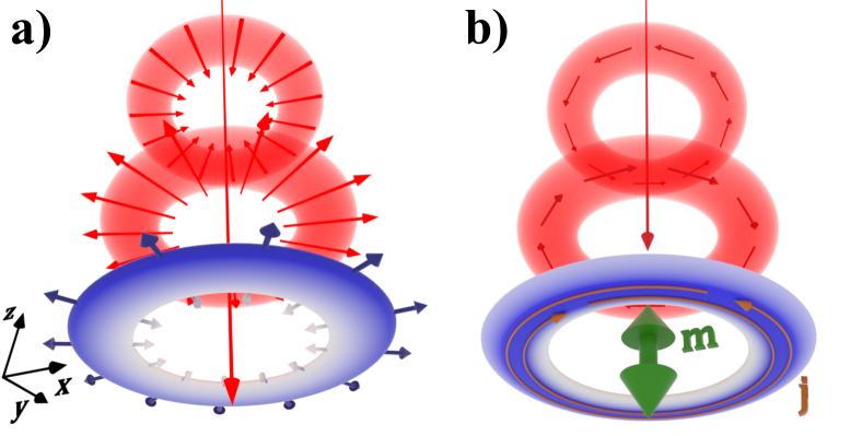
Figure 1: Quantum ring (charge density is marked blue) irradiated by a cylindrical vector beam (red rings at two different times). (a) The radially polarized vector beam initiates electric-type transitions leading to uniform radially breathing charge density. (b) The azimuthally polarized vector beam generates homogeneous oscillating transient currents (orange arrows) giving rise to an oscillating magnetic dipole moment (green arrow). The frequency is set by the driving field.

III.1 Electric Transitions Induced by Radially Polarized Vector beams

The interaction of RVB with quantum rings is illustrated schematically in Figure 1a. The coupling to the electric charge is dominant causing photo-induced transitions, meaning that $\hat{H}^{\rm RVB}_{\rm int}(t)=\hat{H}^{\rm RVB}_{\rm elec}(t)$. Positioning the nano-structure in the plane $z=0$, the interaction with the RVB associated magnetic field (cf. fields in the SI) reads $\hat{H}^{\rm RVB}_{\rm magn}(t)=-2\mathrm{i}\mu_{B}B^{\prime}(\boldsymbol{r},t)(z\partial_{\rho}-\rho\partial_{z})$. Obviously this has no influence on the confined electrons in the $xy$ plane as long as the photon energy $\hbar\omega$ is smaller than the level spacing of the subbands associated with the confinements in the $z$-direction (characterized by $U(z)$). RVBs induce electric transitions between states with an amplitude

$$\begin{split}M^{\rm RVB}_{\rm int}(t)&=\langle\Psi_{m^{\prime}}^{s^{\prime}}|\hat{H}^{\rm RVB}_{\rm el}(t)|\Psi_{m}^{s}\rangle\\ &=\frac{eA_{0}\omega}{q_{\perp}}(J_{0}(q_{\perp}\rho_{0})-1)\sin(\omega t)\quad\delta_{m^{\prime},m}\delta_{s^{\prime},s}.\end{split}$$ (20)

Notably, no direct spin-flip transitions are induced by RBVs; and, in contrast to OAM carrying optical vortex, no orbital angular momentum is transferred to the charge carriers, leading to the selection rule $\Delta m=0$. Thus, in strictly 1D quantum ring angular momentum and spin states are unaffected by RVB. For 2D quantum rings $n\to n^{\prime}$ radial subband transitions are possible with an amplitude (time-averaged and to a first order in the driving fields) proportional to the integral

$$\int_{0}^{\infty}\mathrm{d}\rho\,R_{n^{\prime}m}(\rho)R_{nm}(\rho)(J_{0}(q_{\perp}\rho)-1).$$ (21)

This radial electric excitation has a volume character: The evaluated local dipole moment is the same in all radial directions $\hat{e}_{\rho}$ and oscillates with a frequency characterized by the energy difference between both levels $n$ and $n^{\prime}$. As a result, the averaged total moment is zero:

$$\boldsymbol{d}(t)=\int\mathrm{d}\boldsymbol{r}\,\rho_{e}(\boldsymbol{r},t)\cdot\boldsymbol{r}=0$$ (22)

where $\rho_{e}(\boldsymbol{r},t)$ is the (driven) time-dependent charge density.

For detailed and reliable insight, we performed full-numerical space-time-grid propagation of the three energetically lowest electron states in an irradiated quantum ring including the external fields to all orders. Figure 2(a) displays the resulting charge dynamics induced by the depicted few-cycle external RVB pulse. The ring radius is $\rho_{0}=50$ nm and the effective width $\Delta\rho=30$ nm. The RVB temporal envelope function $\Omega(t)=\sin[\pi t/T_{p}]^{2}$, where $T_{p}=2\pi n_{p}/\omega$ sets the pulse length in terms of the number of optical cycles $n_{p}$. We consider a short pulse with $n_{p}=6$ cycles and a photon energy $\hbar\omega=8$ meV. The small nano-structure is localized in the low-intense beam center and away from the first field intensity maximum. Strong multi-photon processes and the ponderomotive contribution due to $\boldsymbol{A}^{2}(\boldsymbol{r},t)$ we found be negligibly small for the light intensity on the ring which was in the range of $\sim 10^{4}$ W/cm². As predicted by the analytical treatment, we found that all the propagated wave functions keep the symmetry in the azimuthal direction at all times. Field-induced effects are caused by transitions to the second radial subband leading to charge "breathing" oscillations in radial direction (we start from the initial states $n=0,\,m=-1,0,1$). The time-dependent radial expectation value $\langle\rho\rangle$(t) oscillates with a frequency related to $(E_{n=1,m}-E_{n=0,m})/\hbar$. When the pulse is off, the prodded charge dynamics goes on due to coherences meaning that every electron state oscillates between lowest two radial levels.

III.2 Magnetic Transitions Induced by Azimuthally Polarized Vector Beams

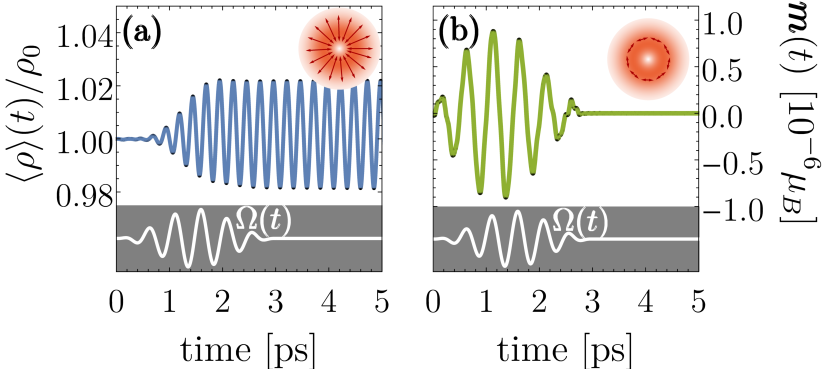
Figure 2: Dynamics from full numerical quantum simulation: (a) time-dependent averaged value $\langle\rho\rangle(t)$ of a quantum ring driven by RVB with six optical cycle duration causing a radial dipole excitation. The oscillation frequency can be identified by $(E_{n=1}-E_{n=0})/\hbar$. (b) The time-dependent magnetic moment in $z$-direction of a quantum ring driven by AVB. The white curves represent the normalized electric field amplitude of the incident light pulses having an intensity $I\sim 10^{4}$ W /cm² in the area of the ring, and $\hbar\omega=8$ meV.

A schematics of an AVB and its action on a quantum ring is shown in Figure 1(b). It is straightforward to demonstrate that the associated electric contribution to the light-matter Hamiltonian $\hat{H}_{\rm int}(t)$ vanishes in the geometry depicted in Figure 1(b): the electric field is perfectly azimuthally polarized and therefore $\boldsymbol{r}\cdot\boldsymbol{E}^{\prime}(\boldsymbol{r},t)\equiv 0$. Thus, the AVB induces no electric (dipole) moment.

The light-matter interaction Hamiltonian reduces to $\hat{H}_{\rm int}(t)\equiv\hat{H}_{\rm magn}^{\text{\tiny AVB}}(t)$. Note, the contribution to the magnetic interaction of the type $\hat{e}_{z}\cdot\hat{\boldsymbol{m}}_{B}=-\mathrm{i}\mu_{B}\partial_{\varphi}$ does not affect the magnetic quantum number, i.e. the selection rule $\Delta m=0$ is obtained. Generally, the interaction matrix elements have the explicit form

$$\begin{split}M_{\rm int}^{\text{\tiny AVB}}(t)&=\langle\Psi_{m^{\prime}}^{s^{\prime}}|\hat{H}^{\text{\tiny AVB}}_{\rm magn}(t)|\Psi_{m}^{s}\rangle\\ &=\mu_{B}\frac{A_{0}}{\rho_{0}}J_{1}(q_{\perp}\rho_{0})\sin(\omega t)\delta_{m^{\prime},m}\left[\left(m+\frac{1}{2}-\frac{1}{2}s\cos(\gamma)\right)\delta_{s^{\prime},s}+\frac{1}{2}\sin(\gamma)\delta_{s^{\prime},-s}\right].\end{split}$$ (23)

Importantly, in contrast to the RVB, spin-flip can be triggered by AVB (recall that the eigenstates of $\hat{H}_{0}$ are not eigenstates of $\sigma_{z}$ nor $\hat{L}_{z}$; thus, for instance $\partial_{\varphi}\Psi_{m}^{s}(\varphi)=\mathrm{i}(m+1/2)\Psi_{m}^{s}(\varphi)-\frac{\mathrm{i}s}{2\sqrt{2\pi}}\mathrm{e}^{\mathrm{i}(m+1/2)\varphi}\nu^{s}(-\gamma,\varphi)$). Further, the spin-flip transitions are proportional to the Rashba coefficient $\sin(\gamma)\propto\alpha_{R}$ (cf. Refs. Zhu and Berakdar (2008); Quinteiro et al. (2011) for EM homogeneous or OAM pulses).

For $\gamma\rightarrow 0$ and starting from equi-populated clock and anti-clockwise angular momentum quantum numbers $m=-M,-M+1,\dots,M-1,M$ (such as the ground state) the induced current density (meaning due to the perturbed states $\delta\Psi_{m}(t)$) reads

$$\begin{split}\boldsymbol{j}(\boldsymbol{r},t)&=\mathbf{j}_{\rm charge}(\boldsymbol{r},t)+\mathbf{j}_{\rm A}(\boldsymbol{r},t),\\ &=\frac{\hbar}{m_{0}\rho_{0}}\sum_{m=-M}^{M}\left\{\Im\left\{\delta\Psi_{m}^{*}(\boldsymbol{r},t)\partial_{\mathbf{\varphi}}\delta\Psi_{m}(\boldsymbol{r},t)\right\}-\frac{e}{m_{0}}\boldsymbol{A}_{\rm AVB}(\boldsymbol{r},t)\left|\delta\Psi_{m}(\boldsymbol{r},t)\right|^{2}\right\},\\ &=\frac{eA_{0}}{m_{0}}J_{1}(q_{\perp}\rho_{0})\delta\rho_{e}\sin(\omega t)\hat{e}_{\varphi}.\end{split}$$ (24)

Obviously, the $\pm M$ state pair deliver the same (in magnitude) but counter-directed current densities and hence $\textbf{j}_{\rm charge}(\boldsymbol{r},t)$ vanishes. Thus, the current density in the $\varphi$-direction is solely set by the induced charge density $\delta\rho_{e}=\sum_{m=-M}^{M}\left|\delta\Psi_{m}(\boldsymbol{r},t)\right|^{2}$ driven by the vector potential $\boldsymbol{A}_{\rm AVB}(\boldsymbol{r},t)$. It follows that $\delta\rho_{e}$ oscillates with the frequency of the driving field which means that, beyond transient effects, no directional time-averaged current is induced. Since the setup can be tuned to low frequencies, the effect should be observable. Note, for the AVB the coupling to the electric field component of light-matter interaction vanishes. Therefore, the resulting oscillating current caused solely by the time-dependent magnetic vector potential $\boldsymbol{A}_{\rm AVB}(\boldsymbol{r},t)$ falls thus in the class of a dynamic Aharonov–Bohm effect.

Since at all time $\boldsymbol{\nabla}\cdot\boldsymbol{j}(\boldsymbol{r},t)\equiv 0$, the continuity equation states that the incident light field does not change the electronic density, i.e. $\partial_{t}\rho(\boldsymbol{r},t)=0$ and our system remains locally and at all time neutral and so does not couple to the electric field part of AVB. Experimentally, we may sense the action of AVB by measuring the associated oscillating magnetic dipole moment

$$\begin{split}\boldsymbol{m}(t)&=\frac{1}{2}\int\mathrm{d}\boldsymbol{r}\,\boldsymbol{r}\times\boldsymbol{j}(\boldsymbol{r},t)\\ &=\frac{e^{2}A_{0}\rho_{0}}{m_{0}}J_{1}(q_{\perp}\rho_{0})\delta\rho_{e}\sin(\omega t)\hat{e}_{z}.\end{split}$$ (25)

In Figure 2(b) the time-dependent magnetic moment in $z$-direction which is gathered from a full numerical quantum dynamic simulation is shown. For the irradiated quantum ring we used the same parameters as for the RVB case. In line with the analytical predictions eq (24), the build-up and decay times are locked to the applied external field pointing to a vanishing contribution $\pm{j}_{\rm charge}(\boldsymbol{r},t)$ to the whole current density (cf. eq (24)). The transient $\boldsymbol{m}(t)$ vanishes once the pulse is off but one may induce also an interference-driven quasi-static component by a combination of two AVB with the frequencies $\omega$ and $2\omega$ (not shown here).

The spin-orbit coupling $\hat{H}_{\rm SOI}(t)$ (cf. eq (11)) is mainly determined by the longitudinal component of the magnetic field of the AVB. The corresponding matrix elements take on the explicit form

$$\begin{split}M^{\text{\tiny AVB}}_{\rm SOI}(t)&=\langle\Psi_{m^{\prime}}^{s^{\prime}}|\hat{H}^{\text{\tiny AVB}}_{\rm SOI}(t)|\Psi_{m}^{s}\rangle\\ &=\frac{e\alpha A_{0}}{\hbar}J_{1}(q_{\perp}\rho_{0})\left[s\sin(\gamma)\delta_{s^{\prime},s}\right.\\ &\quad\left.+\cos(\gamma)\delta_{s^{\prime},-s}\right]\sin(\omega t)\delta_{m^{\prime},m}.\end{split}$$ (26)

Thus, effectively AVB results in spin-flip transitions, even to a first order in the light-matter interaction. The strength of these transitions is linear in SOI strength $\alpha_{R}$. The matrix element indicates that even in the presence SOI the AVB does not cause a change in the angular momentum state. This fact allows to study pure spin dynamics while the orbital angular momentum is frozen. We conclude so that a ubiquitous feature of all vector beam types is that the orbital angular momentum of the electronic states is unaffected.

The further spin-dependent contribution to the AVB-matter interaction is given by $\hat{H}_{\rm z}(t)$. It describes the direct interaction of the spin state with the magnetic field component of the vector beam. Generally, it is much weaker than the spin-orbit interaction, as follows from comparing the prefactors ($e\alpha/\hbar>\mu_{B}q$). Nonetheless, for completeness we provide an expression for the matrix elements of this light-matter interaction contribution. Notice, the magnetic field of the AVB has also a transverse component which couples to $\sigma_{r}$ leading again to spin-flip transitions. In addition to that, the strong longitudinal field (characterized by $J_{0}(q_{\perp}\rho)$) gives rise to a dynamical Zeeman effect. The matrix elements can be found analytically and read explicitly

$$\begin{split}M_{\rm z}^{\text{\tiny AVB}}(t)&=\langle\Psi_{m^{\prime}}^{s^{\prime}}|H^{\rm AVB}_{\rm z}|\Psi_{m}^{s}\rangle,\\ &=\frac{1}{2}g_{s}\mu_{B}A_{0}\left[q_{\parallel}J_{1}(q_{\perp}\rho_{0}\left(s\sin(\gamma)\delta_{s^{\prime},s}+\cos(\gamma)\delta_{s^{\prime},-s}\right)\cos(\omega t)\right.\\ &\quad\left.+q_{\perp}J_{0}(q_{\perp}\rho_{0})\left(s\cos(\gamma)\delta_{s^{\prime},s}-\sin(\gamma)\delta_{s^{\prime},-s}\right)\sin(\omega t)\right]\delta_{m^{\prime},m}.\end{split}$$ (27)

In practice, both spin-orbit coupling contributions bring about dynamical spin flip processes while the individual charge currents (associated with the orbital motion) sum up to zero.

IV Atoms Driven by Vector Beams

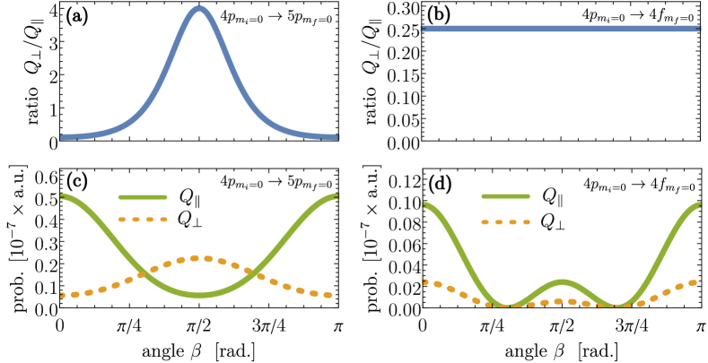
Figure 3: Quadrupole transitions initiated by a vector laser pulse with a radial polarization. A comparison between the longitudinal and the transverse field contributions is shown. Upper row: The ratio between the quadrupole excitation probability, labeled by $Q_{\perp}$ and $Q_{\parallel}$, for the $p$-$p$ and $p$-$f$ transitions. Lower row: Explicit quadrupole excitation probabilities for the $p$-$p$ and $p$-$f$ transitions. The field has a peak intensity of $I=3.51\times 10^{16}$ W/cm². The atom is on the optical access and experience a much lower intensity. The photon energy is tuned to $\hbar\omega=4.37$ eV (for $p$-$p$ transitions) or $\hbar\omega=5.31$ eV ($p$- $f$ transitions); all fields have a duration corresponding of thirty optical cycles. The static magnetic field is set to $10$ T.

Let us consider as a further case an atomic system in a strong magnetic field such that SOI is subsidiary compared to $\mu_{B}B_{z}(\hat{L}_{z}+g_{s}\hat{S}_{z})$ (Paschen–Back effect). The electron states with the usual notation $|i\rangle=|n_{i}\ell_{i}m_{i}s_{i}\rangle$ are appropriate. The magnetic field sets the quantization axis ($z$ axis) while the optical axis of the incident VB makes an angle $\beta=\measuredangle(\hat{e}_{z},q_{\parallel})$ with the $z$ axis. We inspect Rydberg states $|i\rangle$ characterized by the principle, orbital, and magnetic quantum numbers $n_{i}$, $\ell_{i}$ and $m_{i}$. For photoexcitation of higher Rydberg states, as already demonstrated for a trapped ⁴⁰Ca⁺ ion by means of OAM vortex field Schmiegelow et al. (2016), the laser photon energy is such that the wave vector $q=\omega/c\ll 1$ and thus we expand the oscillating functions in Eqs. (3) and (2) in a Taylor series up to terms of the first order: $J_{1}(x)=(1/2)x+\mathcal{O}(x^{3})$, $J_{0}=1+\mathcal{O}(x^{2})$ and $\exp(\mathrm{i}x)=1+\mathrm{i}x+\mathcal{O}(x^{2})$. In the local frame $\left\{\rho^{\prime},\varphi^{\prime},z^{\prime}\right\}$ rotated by $\beta$ relative to the $z$ axis, we employ the rotating wave approximation and obtain for the first-order term of the field of the RVB

$$\begin{split}\boldsymbol{A}_{\rm RVB}(\boldsymbol{r}^{\prime},t)\approx-A_{0}\left[\frac{1}{2}q_{\perp}\rho^{\prime}\hat{e}_{\rho^{\prime}}+\mathrm{i}\frac{q_{\perp}}{q_{\parallel}}(1+\mathrm{i}q_{\parallel}z^{\prime})\hat{e}_{z^{\prime}}\right]e^{-\mathrm{i}\omega t}.\end{split}$$ (28)

Interestingly, the quadrupole terms, originating from the longitudinal and the transverse field distributions have the same prefactors.

Figure 3 shows the results for the photoexcitation process of a trapped Ca⁺ ion starting from the initial $4p_{m_{i}=0}$ Rydberg state by a continuous wave (CW) RVB.

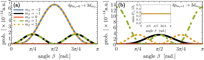
Figure 4: Dipole transitions initiated by an azimuthally polarized vector laser pulse. The population of different magnetic sublevels in dependence on the rotation angle $\beta$ between the beam optical axis and the direction of an external static magnetic field. Two initial states $4p_{m_{i}=0}$ and $4p_{m_{i}=1}$ are shown. Inset: The ratio between the dipole transition probabilities originating from the longitudinal and the transverse field contributions, labeled by $D_{\perp}$ and $D_{\parallel}$. Similar field parameters where used as for Figure 3.

The nature of the matter interaction with a radially polarized vector beam is dominantly electric and is characterized by a strong dipole term stemming from the (electric) longitudinal component. However, one can discriminate between these dipolar and higher order electron transitions by adjusting appropriately the photon energy to $\hbar\omega=\varepsilon_{5p}-\varepsilon_{4p}$ or $\hbar\omega=\varepsilon_{4f}-\varepsilon_{4p}$. The peak amplitude of the vector beam was chosen to be $A_{0}=1$ a.u.. In the region of the atom, however, this amplitude is very small (the prefactor for the transverse electric field is $A_{0}\omega q_{\perp}$ and for the longitudinal field $A_{0}\omega\tan\alpha$ with $\alpha=1^{\circ}$). The left panels on Figure 3 show the quadrupole transition probabilities $Q_{\perp}$ and $Q_{\parallel}$, resolved for the longitudinal and transverse field components, in dependence on the rotation angle $\beta$ for the initial-final state transition $4p_{m_{i}=0}\rightarrow 5p_{m_{f}=0}$. Interestingly, for the orbital momentum conserving quadrupole transition with $\Delta\ell=\Delta m=0$ the ratio $Q_{\perp}/Q_{\parallel}$ can be steered by rotating the incident vector field relative to the applied magnetic field (which sets the quantization axis). Parallel to the magnetic field, the ratio $Q_{\perp}/Q_{\parallel}=1/9$ reveals the dominating longitudinal component while at an angle of $\beta=90^{\circ}$ (RVB and magnetic field are perpendicularly polarized) the transverse component dominates the photoexcitation process since $Q_{\perp}/Q_{\parallel}=4$. Therefore, in contrast to a conventional Gaussian mode we can find angular momentum conserving quadrupole transitions for all possible light field setups due to the special spatially inhomogeneous character of the vector beam.

The situation changes when exploring the $4p_{m_{i}=0}\rightarrow 4f_{m_{f}=0}$ quadrupole transition which is characterized by $\Delta\ell=2$. Here, it is not possible to change the ratio between the longitudinal and transverse field contributions since $Q_{\perp}/Q_{\parallel}=1/4$ for all rotation angles $\beta$. Interestingly, we find rotating angles where the quadrupole transitions (either from the longitudinal or transverse field) vanishes completely. For such a setup the whole photoexcitation probability of $4p_{m_{i}=0}\rightarrow 4f_{m_{f}=0}$ collapses.

For the azimuthal polarization the interaction is fully magnetic since $\boldsymbol{r}\cdot\hat{e}_{\varphi}^{\prime}=0$ and, therefore, we have no coupling to the electron (note that $\boldsymbol{r}\cdot\hat{e}_{\varphi}^{\prime}$ vanishes for every rotation angle $\beta$). With same approximations as for the RVB the strong longitudinal field is given (up to the first order in $r$) by $B_{\parallel}(\boldsymbol{r}^{\prime},t)=\mathrm{i}A_{0}q_{\perp}(1+\mathrm{i}q_{\parallel}z^{\prime})e^{-\mathrm{i}\omega t}\hat{e}_{z}^{\prime}$ while the transverse field $B_{\perp}(\boldsymbol{r}^{\prime},t)=\frac{1}{2}A_{0}q_{\perp}q_{\parallel}\rho^{\prime}e^{-\mathrm{i}\omega t}{e}_{\rho}^{\prime}$. The homogeneous term in the longitudinal component provides no contribution to the photo-induced electron transition since it characterizes a monopole interaction. Consequently, as for the electric type transitions in the case of the RVB the effective contributions of the longitudinal and transverse field components are on equal footing but the associated light-matter interaction is dipolar.

In Figure 4 we show the dipole transitions initiated by the spatially inhomogeneous magnetic field of the AVB for two different initial states $4p_{m_{i}=0}$ and $4p_{m_{f}=1}$. As expected, for $\beta=0^{\circ}$ no photoexcitation processes can be observed since the magnetic field does not act on the electron states with zero angular velocity ($m_{i}=0$). However, as inferred from Figure 4(a), for finite rotating angles one can populate final magnetic substates with $m_{f}\neq 0$. Prominent setups are given by $\beta=\pm 45^{\circ}$ where states with $m_{f}=\pm 1$ and $m_{f}=\pm 2$ are equally excited while for $\beta=\pm 90^{\circ}$ the final states are fully characterized by $m_{f}=\pm 2$. Note, that due to the presence of the external magnetic field, which sets the quantization axis and shifts the energy of the individual magnetic substates (Zeeman effect), the photon energy of the incident AVB has to be adjusted to the specific transitions, i.e. $\hbar\omega=\varepsilon_{n_{f}\ell_{f}m_{f}}-\varepsilon_{n_{i}\ell_{i}m_{i}}$.

In Figure 4(b) the dipolar photoexcitation transitions are depicted for the initial state $4p_{m_{i}=1}$. As expected for $\beta=0^{\circ}$, the only state which can be excited is characterized by $m_{f}=1$ since in this case the interaction between the electron and the light field is angular momentum conserving, i.e. $\Delta m=0$. Interestingly, at $\beta=\pm 90^{\circ}$ the photoexcitation probability of $m_{f}=\pm 1$ is the same while at $\beta=\pm 45^{\circ}$ the dominating final state is characterized by the magnetic quantum number $m_{f}=2$. Another striking feature, in contrast to the RVB, is the ratio between transverse and longitudinal field contributions which is always given by $D_{\perp}/D_{\parallel}=0.25$ and thus, can not be manipulated by the rotation angle $\beta$.

V Summary and outlook

We explored the nature of the interaction of atomic and low dimensional quantum systems (rings) with EM fields with spatially inhomogeneous polarization states, called vector beams. In particular, we focused on cylindrical beams with radial or azimuthal polarization. Although these beams share some common features with vortex beams carrying orbital angular momentum, like the intensity profile, their effect on charge carriers is fundamentally different. For the investigated systems, radially polarized vector beams (RVB) trigger via electric transitions radial charge oscillations. Azimuthally polarized vector beams (AVB) generate via a magnetic interaction oscillating magnetic moments. Despite the presence of the electric field in AVB, it subsumes in a way that it does not affect the charge. The interaction with AVB is solely due to the magnetic vector potential, and can thus be interpreted as a dynamic Aharonov–Bohm effect. In contrast to OAM carrying fields, no unidirectional, time averaged currents are generated by AVB nor by RVB. Atomic targets subject to radially polarized light fields show angular momentum conserving quadrupole transitions which can be manipulated in magnitude by rotating the field relative to the quantization axis set by an external static magnetic field. When photoexciting with an azimuthally polarized field, the special field structure makes it possible to select different magnetic sublevels (in the final state) by rotating the laser field relative to the quantization axis of the atomic target.

VI Acknowledgements

This work was partially supported by the DFG through SPP1840 and SFB TRR 227.

Appendix A

The electric field of a radially polarized vector beam (RVB) is given by

$$E_{r}^{\rm RVB}(\boldsymbol{r},t) =A_{0}\omega_{x}J_{1}(q_{\perp}\rho)\sin(q_{\parallel}z-\omega_{x}t),$$ (29a)

$$E_{\varphi}^{\rm RVB}(\boldsymbol{r},t) =0,$$ (29b)

$$E_{z}^{\rm RVB}(\boldsymbol{r},t) =A_{0}\omega_{x}\frac{q_{\perp}}{q_{\parallel}}J_{0}(q_{\perp}\rho)\cos(q_{\parallel}z-\omega_{x}t),$$ (29c)

while the associated magnetic field reads

$$B_{r}^{\rm RVB}(\boldsymbol{r},t) =0,$$ (30a)

$$B_{\varphi}^{\rm RVB}(\boldsymbol{r},t) =A_{0}\frac{q_{\perp}^{2}+q_{\parallel}^{2}}{q_{\parallel}}J_{1}(q_{\perp}\rho)\sin(q_{\parallel}z-\omega_{x}t),$$ (30b)

$$B_{z}^{\rm RVB}(\boldsymbol{r},t) =0.$$ (30c)

In the same vein, the electromagnetic fields of the azimuthally polarized vector beam (AVB) as the sum of two antiparallel Bessel beams read

$$E_{r}^{\rm AVB}(\boldsymbol{r},t) =0,$$ (31a)

$$E_{\varphi}^{\rm AVB}(\boldsymbol{r},t) =-A_{0}\omega_{x}J_{1}(q_{\perp}\rho)\cos(q_{\parallel}z-\omega_{x}t),$$ (31b)

$$E_{z}^{\rm AVB}(\boldsymbol{r},t) =0,$$ (31c)

and

$$B_{r}^{\rm AVB}(\boldsymbol{r},t) =A_{0}q_{\parallel}J_{1}(q_{\perp}\rho)\cos(q_{\parallel}z-\omega_{x}t),$$ (32a)

$$B_{\varphi}^{\rm RVB}(\boldsymbol{r},t) =0,$$ (32b)

$$B_{z}^{\rm AVB}(\boldsymbol{r},t) =-A_{0}q_{\perp}J_{0}(q_{\perp}\rho)\sin(q_{\parallel}z-\omega_{x}t),$$ (32c)

Appendix B

Using the vector potential in the Poincaré gauge, i.e. $\boldsymbol{A}^{\prime}(\boldsymbol{r},t)=-\boldsymbol{r}\times\int_{0}^{1}\mathrm{d}\lambda\,\lambda\boldsymbol{B}(\lambda\boldsymbol{r},t)$ where the vector field satisfies $\boldsymbol{r}\cdot\boldsymbol{A}^{\prime}(\boldsymbol{r},t)\equiv 0$, we derive the expression for the magnetic contribution to the interaction Hamiltonian $\hat{H}_{\rm int}(t)$ from the minimal coupling scheme:

$$H_{\rm magn}(t)=-\frac{e}{2m_{0}}\left(\boldsymbol{p}\cdot\boldsymbol{A}^{\prime}(\boldsymbol{r},t)+\boldsymbol{A}^{\prime}(\boldsymbol{r},t)\cdot\boldsymbol{p}\right).$$ (33)

Inserting $\boldsymbol{A}^{\prime}(\boldsymbol{r},t)$ as well as applying the fundamental identities $\boldsymbol{p}\cdot\left(\boldsymbol{r}\times\boldsymbol{B}\right)=\left(\boldsymbol{p}\times\boldsymbol{r}\right)\cdot\boldsymbol{B}$ as well as $\left(\boldsymbol{r}\times\boldsymbol{B}\right)\cdot\boldsymbol{p}=\boldsymbol{B}\cdot\left(\boldsymbol{p}\times\boldsymbol{r}\right)$, we find

$$H_{\rm magn}(t)=\frac{e}{2m_{0}}\left(\boldsymbol{p}\times\boldsymbol{r}\right)\cdot\int_{0}^{1}\mathrm{d}\lambda\,\lambda\boldsymbol{B}(\lambda\boldsymbol{r},t)+\frac{e}{2m_{0}}\int_{0}^{1}\mathrm{d}\lambda\,\lambda\boldsymbol{B}(\lambda\boldsymbol{r},t)\cdot\left(\boldsymbol{p}\times\boldsymbol{r}\right).$$ (34)

From elementary quantum mechanical algebra we know that

$$\left(\boldsymbol{p}\times\boldsymbol{r}\right)\cdot\boldsymbol{B}=\boldsymbol{B}\cdot\left(\boldsymbol{p}\times\boldsymbol{r}\right)-\left[\boldsymbol{B},\left(\boldsymbol{p}\times\boldsymbol{r}\right)\right]_{-}.$$ (35)

Using $\boldsymbol{p}\times\boldsymbol{r}=-\boldsymbol{r}\times\boldsymbol{p}$ and we can find the commutator

$$\begin{split}\left[\boldsymbol{B},\left(\boldsymbol{p}\times\boldsymbol{r}\right)\right]_{-}&=\left[\left(\boldsymbol{r}\times\boldsymbol{p}\right),\boldsymbol{B}\right]_{-}\\ &=\varepsilon_{ijk}\left[x_{j}p_{k},B_{i}\right]_{-}\\ &=\varepsilon_{ijk}x_{j}\left[p_{k},B_{i}\right]_{-}+\varepsilon_{ijk}\underbrace{\left[x_{j},B_{i}\right]_{-}}_{=0}p_{k}\\ &=\boldsymbol{r}\cdot(\boldsymbol{p}\times\boldsymbol{B}).\end{split}$$ (36)

By using now Ampère–Maxwell law Jackson (1975) the commutator can be reformulated further:

$$\begin{split}\left[\boldsymbol{B},\left(\boldsymbol{p}\times\boldsymbol{r}\right)\right]_{-}&=\boldsymbol{r}\cdot(\boldsymbol{p}\times\boldsymbol{B})\\ &=-\mathrm{i}\hbar\boldsymbol{r}\cdot\left[\boldsymbol{\nabla}\times\boldsymbol{B}(\boldsymbol{r},t)\right]\\ &=-\frac{\mathrm{i}\hbar}{c^{2}}\boldsymbol{r}\cdot\frac{\partial\boldsymbol{E}(\boldsymbol{r},t)}{\partial t}.\end{split}$$ (37)

Furthermore, by assuming a harmonic wave we find that $\partial_{t}\boldsymbol{E}(\boldsymbol{r},t)\sim-\omega_{x}\boldsymbol{E}(\boldsymbol{r},t)$ and obtain the final expression for Hamiltonian containing the commutator

$$\begin{split}H_{\rm magn}^{\rm comm.}&=-\int_{0}^{1}\mathrm{d}\lambda\,\lambda\frac{e}{2m}\left[\boldsymbol{B},\left(\boldsymbol{p}\times\boldsymbol{r}\right)\right]_{-}\\ &=\frac{\mathrm{i}e}{2}\frac{\hbar\omega_{x}}{m_{0}c^{2}}\int_{0}^{1}\mathrm{d}\lambda\,\lambda\boldsymbol{r}\cdot\boldsymbol{E}(\boldsymbol{r},t),\end{split}$$ (38)

which can be safely neglected by noticing that the prefactor $\hbar\omega_{x}/m_{0}c^{2}<10^{-4}$ even for photon energies in the (X)UV regime. Furthermore, in the case of an AVB $\boldsymbol{r}\cdot\boldsymbol{E}(\boldsymbol{r},t)\equiv 0$ (azimuthal polarization). As a consequence, the magnetic part of the interaction Hamiltonian is

$$\begin{split}H_{\rm magn}(t)&=\frac{e}{m_{0}}\left[-\int_{0}^{1}\mathrm{d}\lambda\,\lambda\boldsymbol{B}(\lambda\boldsymbol{r},t)\right]\cdot\left(\boldsymbol{r}\times\hat{\boldsymbol{p}}\right)\\ &=2\boldsymbol{B}^{\prime}(\boldsymbol{r},t)\cdot\widehat{\boldsymbol{m}}_{B}\end{split}$$ (39)

where $\boldsymbol{B}^{\prime}(\boldsymbol{r},t)=-\int_{0}^{1}\mathrm{d}\lambda\,\lambda\boldsymbol{B}(\lambda\boldsymbol{r},t)$ and the magnetic moment operator is $\widehat{\boldsymbol{m}}_{B}=(e/2m)\,\boldsymbol{r}\times\hat{\boldsymbol{p}}$.

References

- Brabec and Krausz (2000) T. Brabec and F. Krausz, Rev. Mod. Phys. 72, 545 (2000).
- Petek and Ogawa (1997) H. Petek and S. Ogawa, Prog. Surf. Sci. 56, 239 (1997).
- Ng et al. (2010) J. Ng, Z. Lin, and C.T. Chan, Phys. Rev. Lett. 104, 103601 (2010).
- Hao et al. (2010) X. Hao, C. Kuang, T. Wang, and X. Liu, Opt. Lett. 35, 3928 (2010).
- Dorn et al. (2003) R. Dorn, S. Quabis, and G. Leuchs, Phys. Rev. Lett. 91, 233901 (2003).
- Kang et al. (2012) M. Kang, J. Chen, X.-L. Wang, and H.-T. Wang, JOSA B 29, 572 (2012).
- Bauer et al. (2014) T. Bauer, S. Orlov, U. Peschel, P. Banzer, and G. Leuchs, Nat. Photonics 8, 23 (2014).
- Parigi et al. (2015) V. Parigi, V. DÁmbrosio, C. Arnold, L. Marrucci, F. Sciarrino, and J. Laurat, Nat. Commun. 6, 7706 (2015).
- Dámbrosio et al. (2012) V. Dámbrosio, E. Nagali, S. P. Walborn, L. Aolita, S. Slussarenko, L. Marrucci, and F. Sciarrino, Nat. Commun. 3, 961 (2012).
- Vallone et al. (2014) G. Vallone, V. DÁmbrosio, A. Sponselli, S. Slussarenko, L. Marrucci, F. Sciarrino, and P. Villoresi, Physical review letters 113, 060503 (2014).
- Gabriel et al. (2011) C. Gabriel, A. Aiello, W. Zhong, T. G. Euser, N. Y. Joly, P. Banzer, M. Förtsch, D. Elser, U. L. Andersen, C. Marquardt,P. S. J. Russell, and G. Leuchs, Phys. Rev. Lett. 106, 060502 (2011).
- Guclu et al. (2016) C. Guclu, M. Veysi, and F. Capolino, ACS Photonics 3, 2049 (2016).
- Bliokh et al. (2015) K. Y. Bliokh, F. Rodríguez-Fortuño, F. Nori, and A. V. Zayats, Nat. Phot. 9, 796 (2015).
- Schmiegelow et al. (2016) C. T. Schmiegelow, J. Schulz, H. Kaufmann, T. Ruster, U. G. Poschinger, and F. Schmidt-Kaler, Nat. Commun. 7, 12998 (2016).
- Wätzel and Berakdar (2016) J. Wätzel and J. Berakdar, Sci. Rep. 6, 21475 (2016).
- Wätzel et al. (2016) J. Wätzel, Y. Pavlyukh, A. Schäffer, and J. Berakdar, Carbon 99, 439 (2016).
- Zurita-Sánchez and Novotny (2002) J. R. Zurita-Sánchez and L. Novotny, J. Opt. Soc. Am. B 19, 2722 (2002).
- Hanewinkel et al. (1997) B. Hanewinkel, A. Knorr, P. Thomas, and S.W. Koch, Phys. Rev. B 55, 13715 (1997).
- Veysi et al. (2015) M. Veysi, C. Guclu, and F. Capolino, J. Opt. Soc. Am. B 32, 345 (2015).
- Oron et al. (2000) R. Oron, S. Blit, N. Davidson, A. A. Friesemzeev Bomzon, E. Hasman, A. A. Friesem, and Z. Bomzon, Appl. Phys. Lett. 77, 3322 (2000).
- Tidwell et al. (1990) S. C. Tidwell, D. H. Ford, and W. D. Kimura, Appl. Opt. 29, 2234 (1990).
- Churin et al. (1993) E. G. Churin, J. Hobfeld, and T. Tschudi, Opt. Commun. 99, 13 (1993).
- Stalder and Schadt (1996) M. Stalder and M. Schadt, Opt. Lett. 21, 1948 (1996).
- Tripathi and Toussaint (2012) S. Tripathi and K. C. Toussaint, Opt. Expr. 20, 10788 (2012).
- Giovani Milione, Henry I. Sztul, Dan A. Nolan, Jonathan Kim (2011) M. E. Giovani Milione, Henry I. Sztul, Dan A. Nolan, Jonathan Kim, CLEO Sci. Innov. (Optical Society of America, 2011) p. CTuB2.
- Memarzadeh and Mosallaei (2011) B. Memarzadeh and H. Mosallaei, Opt. Lett. 36, 2569 (2011).
- Yu et al. (2011) N. Yu, P. Genevet, M. a. Kats, F. Aieta, J.-P. Tetienne, F. Capasso, and Z. Gaburro, Science 334, 333 (2011).
- Yu et al. (2012) N. Yu, F. Aieta, P. Genevet, M. A. Kats, Z. Gaburro, and F. Capasso, Nano Lett. 12, 6328 (2012).
- Bomzon et al. (2002) Z. Bomzon, G. Biener, V. Kleiner, and E. Hasman, Opt. Lett. 27, 285 (2002).
- Beresna et al. (2011) M. Beresna, M. Gecevičius, P. G. Kazansky, and T. Gertus, Appl. Phys. Lett. 98, 1 (2011).
- Yi et al. (2014) X. Yi, X. Ling, Z. Zhang, Y. Li, X. Zhou, Y. Liu, S. Chen, H. Luo, and S. Wen, Opt. Expr. 22, 17207 (2014).
- Liu et al. (2014) Y. Liu, X. Ling, X. Yi, X. Zhou, H. Luo, and S. Wen, Appl. Phys. Lett. 104, 191110 (2014).
- Saito et al. (2008) Y. Saito, M. Kobayashi, D. Hiraga, K. Fujita, S. Kawano, N. I. Smith, Y. Inouye, and S. Kawata, J. Raman Spectrosc. 39, 1643 (2008).
- Wang et al. (2008) H. Wang, L. Shi, B. Lukyanchuk, C. Sheppard, and C. T. Chong, Nat. Photonics 2, 501 (2008).
- Meier et al. (2007) M. Meier, V. Romano, and T. Feurer, Appl. Phys. A Mater. Sci. Process. 86, 329 (2007).
- Zhan (2004) Q. Zhan, Opt. Expr. 12, 3377 (2004).
- Sbierski et al. (2013) B. Sbierski, G. F. Quinteiro, P. I. Tamborenea, Q. Zhan, C. Gabriel, A. Aiello, W. Zhong, T. G. Euser, N. Y. Joly, P. Banzer, M. Förtsch, D. Elser, U. L. Andersen, C. Marquardt, and Others, J. Phys. Condens. Matter 25, 385301 (2013).
- Quinteiro and Kuhn (2014) G. F. Quinteiro and T. Kuhn, Phys. Rev. B 90, 115401 (2014).
- Allen et al. (1992) L. Allen, M. W. Beijersbergen, R. J. C. Spreeuw, and J. P. Woerdman, Phys. Rev. A 45, 8185 (1992).
- Yao and Padgett (2011) A. M. Yao and M. J. Padgett, Adv. Opt. Photonics 3, 161 (2011).
- Quinteiro et al. (2011) G. F. Quinteiro, P. I. Tamborenea, and J. Berakdar, Opt. Expr. 19, 26733 (2011).
- Novotny et al. (1998) L. Novotny, E. J. Sachez, and X. S. Xie, Ultramicroscopy 71, 21 (1998).
- Garces-Chavez et al. (2002) V. Garces-Chavez, J. Arlt, K. Dholakia, K. Volke-Sepulveda, and S. Chavez-Cerda, J. Opt. B Quantum Semiclass. Opt. 4, 82 (2002).
- Cohen-Tannoudji et al. (1989) C. Cohen-Tannoudji, J. Dupont-Roc, and G. Grynberg, Photons and atomso Title (Wiley- Interscience, New York, 1989).
- Cohen-Tannoudji et al. (1992) C. Cohen-Tannoudji, J. Dupont-Roc, G. Grynberg, and P. Thickstun, Atom-photon interactions: basic processes and applications (Wiley Online Library, 1992).
- Quinteiro et al. (2017) G. F. Quinteiro, D. E. Reiter, and T. Kuhn, Phys. Rev. A 95, 012106 (2017).
- Frustaglia and Richter (2004) D. Frustaglia and K. Richter, Phys. Rev. B 69, 235310 (2004).
- Molnár et al. (2005) B. Molnár, P. Vasilopoulos, and F. M. Peeters, Phys. Rev. B 72, 075330 (2005).
- Sheng and Chang (2006) J. S. Sheng and K. Chang, Phys. Rev. B. 74, 235315 (2006).
- Földi et al. (2006) P. Földi, O. Kálmán, M. G. Benedict, and F. M. Peeters, Phys. Rev. B 73, 155325 (2006).
- Zhu and Berakdar (2008) Z. G. Zhu and J. Berakdar, Phys. Rev. B. 77, 235438 (2008).
- Iyoda et al. (2011) M. Iyoda, J. Yamakawa, and M. J. Rahman, Angew. Chem. Int. Ed. Engl. 50, 10522 (2011).
- Choi and Hamilton (2003) K. Choi and A. D. Hamilton, Coord. Chem. Rev. 240, 101 (2003).
- Stoddart (2017) J. F. Stoddart, Angew. Chem. Int. Ed. Engl. 56, 11094 (2017).
- Jackson (1975) J. D. Jackson, Classical electrodynamics (Wiley Online Library, 1975).