The Enskog–Vlasov equation:
A kinetic model describing gas, liquid, and solid

Abstract

The Enskog–Vlasov (EV) equation is a semi-empiric kinetic model describing gas-liquid phase transitions. In the framework of the EV equation, these correspond to an instability with respect to infinitely long perturbations, developing in a gas state when the temperature drops below (or density rises above) a certain threshold. In this paper, we show that the EV equation describes one more instability, with respect to perturbations with a finite wavelength and occurring at a higher density. This instability corresponds to fluid-solid phase transition and the perturbations’ wavelength is essentially the characteristic scale of the emerging crystal structure. Thus, even though the EV model does not describe the fundamental physics of the solid state, it can ‘mimic’ it – and, thus, be used in applications involving both evaporation and solidification of liquids. Our results also predict to which extent a pure fluid can be overcooled before it definitely turns into a solid.

1 Introduction

The Enskog–Vlasov (EV) kinetic equation comprises the Enskog collision integral for dense fluids [Enskog22] and a Vlasov term describing the van-der-Waals force. The first version of the EV equation [Desobrino67] was based on the original form of the Enskog integral – which, as shown in [LebowitzPercusSykes69], does not comply with the Onsager relations. [VanbeijerenErnst73a] proposed a modification of the Enskog integral free from this shortcoming, which was incorporated in the EV model in [KarkheckStell81, StellKarkheckVanbeijeren83]. [GrmelaGarciacolin80] showed that an H-theorem holds for the EV equation only subject to a certain restriction of its coefficients, and [BenilovBenilov18] proposed a version of the EV equation that satisfies this restriction and conserves energy as well (all of the previous versions do not).

Note that, in kinetic models, phase transitions correspond to instabilities. For the original version of the EV equation, the presence of an instability has been shown in [Grmela71], and it was interpreted as gas-liquid phase transition.

In the present paper, we report the results of a more detailed study. Using the EV equation that conserves energy and satisfies an H-theorem, we find two instabilities, with respect to infinite- and finite-wavelength perturbations – interpreted as gas-liquid and fluid-solid transitions, respectively. The latter result comes as a surprise, as the EV equation was conceived as a tool for modeling of fluids only. We show, however, that it admits periodic solutions capable of ‘mimicking’ the solid phase.

The present paper has the following structure. In section 2, we introduce the Enskog–Vlasov equation and, in section 3, carry out the stability analysis of its spatially homogeneous solutions. The general results are illustrated by applying them to noble gases in sections 4–5.

2 The Enskog–Vlasov model

2.1 The EV equation

Consider a fluid of hard spheres of diameter $D$, characterized by the one-particle distribution function $f(\mathbf{r},\mathbf{v},t)$ where $\mathbf{r}$ is the position vector, $\mathbf{v}$ the velocity, and $t$ the time.

Let the molecules exert on each other a force with a pair-wise potential $\Phi(r)$, modeling physically the van der Waals interaction of molecules. Let $\Phi(r)$ be a monotonically growing function of $r$, so that the van der Waals force is attractive at all distances. Letting also, without loss of generality, $\Phi\rightarrow 0$ as $r\rightarrow\infty$, we can assume that $\Phi(r)<0$ for all $r$.

As seen later, the main characteristic of $\Phi$ – one that affects the fluid’s macroscopic properties – is

$$E=-\int\Phi(r)\,\mathrm{d}^{3}\mathbf{r}.$$ (1)

Using $E$, $D$, the molecular mass $m$, and the Boltzmann constant $k_{B}$, we introduce the following nondimensional variables:

$$\mathbf{r}_{nd}=\frac{\mathbf{r}}{D},\qquad\mathbf{v}_{nd}=\left(\frac{m}{ED^{3}}\right)^{1/2}\mathbf{v},\qquad t_{nd}=\left(\frac{ED}{m}\right)^{1/2}t,$$

$$f_{nd}=\frac{k_{B}E^{1/2}D^{3/2}}{m^{3/2}}f,\qquad\Phi_{nd}=\frac{\Phi}{ED^{3}}.$$

Note that, due to (1), the nondimensional potential $\Phi_{nd}$ satisfies (the subscript _nd omitted)

$$\int\Phi(r)\,\mathrm{d}^{3}\mathbf{r}=-1.$$ (2)

In terms of the nondimensional variables, the Enskog–Vlasov equation has the form (_nd omitted)

$$\frac{\partial f(\mathbf{r,v},t)}{\partial t}+\mathbf{v}\cdot\mathbf{\nabla}f(\mathbf{r,v},t)+\mathbf{F}(\mathbf{r},t)\cdot\frac{\partial f(\mathbf{r,v},t)}{\partial\mathbf{v}}$$

$$=\int\int\left[\eta(\mathbf{r},\mathbf{r}+\mathbf{\bm{\kappa}},t)\,f(\mathbf{r},\mathbf{v}^{\prime},t)\,f(\mathbf{r}+\mathbf{\bm{\kappa}},\mathbf{v}_{1}^{\prime},t)\right.$$

$$-\left.\eta(\mathbf{r},\mathbf{r}-\mathbf{\bm{\kappa}},t)\,f(\mathbf{r},\mathbf{v},t)\,f(\mathbf{r}-\mathbf{\bm{\kappa}},\mathbf{v}_{1},t)\right]\mathbf{g}\cdot\mathbf{\bm{\kappa}}\,\mathrm{H}(\mathbf{g}\cdot\mathbf{\bm{\kappa}})\,\mathrm{d}^{2}\mathbf{\bm{\kappa}}\,\mathrm{d}^{3}\mathbf{v}_{1},$$ (3)

where $\mathrm{H}$ is the Heaviside function,

$$\mathbf{F}(\mathbf{r},t)=-\mathbf{\nabla}\int n(\mathbf{r}_{1},t)\,\Phi(\left|\mathbf{r}-\mathbf{r}_{1}\right|)\,\mathrm{d}^{3}\mathbf{r}_{1}$$ (4)

is the collective van der Waals force,

$$n(\mathbf{r},t)=\int f(\mathbf{r},\mathbf{v},t)\,\mathrm{d}^{3}\mathbf{v}$$ (5)

is the number density, $\mathbf{\bm{\kappa}}$ is a unit vector parameterizing all possible orientations of a pair of spheres (molecules) at the moment of collision, and the post-collision velocities $\left(\mathbf{v}^{\prime},\mathbf{v}_{1}^{\prime}\right)$ are related to the pre-collision ones, $\left(\mathbf{v},\mathbf{v}_{1}\right)$, by

$$\mathbf{v}^{\prime}=\mathbf{v}+\mathbf{\bm{\kappa}}\left(\mathbf{g}\cdot\mathbf{\bm{\kappa}}\right),\qquad\mathbf{v}_{1}^{\prime}=\mathbf{v}_{1}-\mathbf{\bm{\kappa}}\left(\mathbf{g}\cdot\mathbf{\bm{\kappa}}\right)\mathbf{,\qquad g}=\mathbf{v}_{1}-\mathbf{v}.$$ (6)

The coefficient $\eta(\mathbf{r},\mathbf{r}_{1},t)$ which appears in the collision integral is, generally, a functional of $n(\mathbf{r},t)$. It originates from the main assumption of the EV theory that the two-particle distribution function $f^{(2)}(\mathbf{r},\mathbf{v},\mathbf{r}_{1},\mathbf{v}_{1},t)$ is related to the singlet $f(\mathbf{r},\mathbf{v},t)$ by

$$f^{(2)}(\mathbf{r},\mathbf{v},\mathbf{r}_{1},\mathbf{v}_{1},t)=\eta(\mathbf{r},\mathbf{r}_{1},t)\,f(\mathbf{r},\mathbf{v},t)\,f(\mathbf{r}_{1},\mathbf{v}_{1},t).$$

Given a specific expressions for $\eta$, equations (3)–(6) fully determine the evolution of $f$.

There are three approaches to choosing $\eta(\mathbf{r},\mathbf{r}_{1},t)$:

1. In the original Enskog theory [Enskog22], $\eta$ is a function of the number density evaluated at the midpoint between the colliding molecules, i.e., $n(\frac{1}{2}(\mathbf{r}+\mathbf{r}_{1}),t)$. This function is supposed to be such that the EV model describes the equation of state (EoS) of the fluid under consideration with the best possible accuracy.

2. The authors of [VanbeijerenErnst73a] derived $\eta$ from a hypothesis that the n-particle distribution function is represented by a product of singlet distributions and (sic!) a factor excluding all states where the hard spheres overlap. This hypothesis does hold at equilibrium, but should be considered as approximate otherwise. Another difficulty associated with this approach is that the resulting $\eta$ is defined through a limiting procedure involving multiple integrals of increasing order, making it impossible to solve the EV equation numerically.

3. The authors of [BenilovBenilov18] assumed

   $$\eta(\mathbf{r},\mathbf{r}_{1},t)=1+\sum_{l=2}^{L}c_{l}\int^{l}\left[{\displaystyle\prod_{i=2}^{l}}n(\mathbf{r}_{i},t)\,\mathrm{H}(1-\left|\mathbf{r}-\mathbf{\mathbf{r}}_{i}\right|)\,\mathrm{H}(1-\left|\mathbf{r}_{1}-\mathbf{\mathbf{r}}_{i}\right|)\right]$$

   $$\times\left[{\displaystyle\prod_{i=2}^{l-1}}\,\,{\displaystyle\prod_{j=i+1}^{l}}\mathrm{H}(1-\left|\mathbf{r}_{i}-\mathbf{\mathbf{r}}_{j}\right|)\right]{\displaystyle\prod_{i=1}^{l}}\mathrm{d}^{3}\mathbf{r}_{i},$$ (7)

   where $\int^{l}$ denotes $l$ repeated integrals, and the coefficients $c_{2}$, $c_{3}$, $c_{4}$…$c_{L}$ are to be chosen to fit the properties of the fluid under consideration. Note that the ‘proper’ hard-sphere $\eta$ derived in [VanbeijerenErnst73a] is a particular case of (7) – one with $L=\infty$ and certain values of $c_{l}$ (which are not easy to calculate).

It turns out that the choice of $\eta$ affects the fundamental properties of the EV equation.

Consider, for example, the entropy of the system, which is traditionally assumed [Desobrino67, GrmelaGarciacolin80, GrmelaGarciacolin80b, Grmela81] to have the form

$$S=-\int\int f(\mathbf{r,v},t)\ln f(\mathbf{r,v},t)\,\mathrm{d}^{3}\mathbf{v}\,\mathrm{d}^{3}\mathbf{r}+Q[n],$$

where the non-ideal contribution $Q[n]$ is a functional depending on $n(\mathbf{r},t)$. Then, the H-theorem holds if and only if $Q[n]$ and $\eta$ are inter-related by

$$\mathbf{\nabla}\frac{\delta Q[n]}{\delta n(\mathbf{r},t)}=-\int\eta(\mathbf{r},\mathbf{r}_{1},t)\,n(\mathbf{r}_{1},t)\,(\mathbf{r}_{1}-\mathbf{\mathbf{r}})\,\delta(\left|\mathbf{r}-\mathbf{\mathbf{r}}_{1}\right|-1)\,\mathrm{d}^{3}\mathbf{r}_{1}$$ (8)

(see [GrmelaGarciacolin80] and, for more detail, Appendix A of [BenilovBenilov18]). The question of existence of $Q[n]$ as a solution of equation (8) for a given $\eta$ is not trivial. If, for example, $\eta$ is a function of $n\left(\frac{1}{2}(\mathbf{r+r}_{1}),t\right)$ – as in the original Enskog’s theory – (8) does not seem to have a solution ofr $Q$. For the versions of $\eta$ suggested in [VanbeijerenErnst73a, BenilovBenilov18], on the other hand, it does. In the latter case, an explicit expression for $Q$ can be found,

$$Q[n]=-\frac{1}{2}\int\int n(\mathbf{r})\,n(\mathbf{r}_{1})\,\mathrm{H}(1-\left|\mathbf{r}-\mathbf{\mathbf{r}}_{1}\right|)\,\mathrm{d}^{3}\mathbf{r}\,\mathrm{d}^{3}\mathbf{r}_{1}$$

$$-\sum_{l=2}^{L}\frac{c_{l}}{l\left(l+1\right)}\int^{l}\int n(\mathbf{r})\left[{\displaystyle\prod_{i=1}^{l}}n(\mathbf{r}_{i})\,\mathrm{H}(1-\left|\mathbf{r}-\mathbf{\mathbf{r}}_{i}\right|)\right]$$

$$\times\left[{\displaystyle\prod_{i=1}^{l-1}}\,\,{\displaystyle\prod_{j=i+1}^{l}}\mathrm{H}(1-\left|\mathbf{r}_{i}-\mathbf{\mathbf{r}}_{j}\right|)\right]\mathrm{d}^{3}\mathbf{r}\,{\displaystyle\prod_{i=1}^{l}}\mathrm{d}^{3}\mathbf{r}_{i},$$ (9)

where the coefficients $c_{l}$ are the same as in expression (7) for $\eta$.

In this paper, we shall use $\eta$ and $Q$ given by (7) and (9), respectively.

We shall also need the function $\Theta(n)$ related to the functional $Q[n]$ by

$$\Theta(n)=-\frac{1}{n}\left(Q[n]\right)_{n=\mathrm{const}},$$

so that (9) yields

$$\Theta(n)=\frac{2\pi}{3}n+\sum_{l=2}^{L}\frac{c_{l}A_{l}}{l\left(l+1\right)}n^{l},$$ (10)

where

$$A_{l}=\int^{l}\left[{\displaystyle\prod_{i=1}^{l}}\mathrm{H}(1-\left|\mathbf{\mathbf{r}}_{i}\right|)\right]\left[{\displaystyle\prod_{i=1}^{l-1}}\,\,{\displaystyle\prod_{j=i+1}^{l}}\mathrm{H}(1-\left|\mathbf{r}_{i}-\mathbf{\mathbf{r}}_{j}\right|)\right]{\displaystyle\prod_{i=1}^{l}}\mathrm{d}^{3}\mathbf{r}_{i}$$ (11)

are numeric constants.

$\Theta(n)$ plays an important role in the thermodynamics of EV fluids: in particular, their EoS is [BenilovBenilov18]

$$p=nT\left[1+n\Theta^{\prime}(n)\right]-\frac{1}{2}n^{2}.$$ (12)

where $\Theta^{\prime}=\mathrm{d}\Theta/\mathrm{d}n$.

2.2 Steady solutions of the EV equation

Physically, steady (time independent) solutions of the EV equation must have spatially uniform temperature and zero fluxes of mass, momentum, and energy – which means that they must be equilibrium states.

To find these, observe that the scattering cross-section in the Enskog integral does not depend on $\mathbf{v}$ – as a result, the EV equation is consistent with the following ansatz:

$$f(\mathbf{r},\mathbf{v},t)=\frac{n(\mathbf{r})}{\left(2\pi T\right)^{3/2}}\exp\left(-\frac{\left|\mathbf{v}\right|^{2}}{2T}\right),$$

where $T$ is the temperature. Substituting this ansatz into the EV equation and carrying out straightforward algebra (see [Grmela71]), we obtain the following equation for $n(\mathbf{r})$:

$$\mathbf{\nabla}\left[\ln n(\mathbf{r})+\frac{1}{T}\int n(\mathbf{r}_{1})\,\Phi(\left|\mathbf{r}-\mathbf{r}_{1}\right|\mathbf{)}\,\mathrm{d}^{3}\mathbf{r}_{1}\right]$$ (13)

$$+\int\eta(\mathbf{r},\mathbf{r}_{1})\,n(\mathbf{r}_{1})\,(\mathbf{r}_{1}-\mathbf{r})\,\delta(\left|\mathbf{r}_{1}-\mathbf{r}\right|-1)\,\mathrm{d}^{3}\mathbf{r}_{1}=0.$$ (14)

Subject to (8), this equation can be integrated,

$$\ln n(\mathbf{r})+\frac{1}{T}\int n(\mathbf{r}_{1})\,\Phi(\left|\mathbf{r}-\mathbf{r}_{1}\right|\mathbf{)}\,\mathrm{d}^{3}\mathbf{r}_{1}-\frac{\delta Q[n]}{\delta n(\mathbf{r})}=\mathrm{const}.$$ (15)

This equation coincides with the Euler equation from density functional theory and also arises in equilibrium statistical mechanics (grand ensemble), where the term involving $\Phi$ is the functional derivative of the mean field contribution to the free energy, the $\mathrm{const}$ is the nondimensional chemical potential divided by $T$, and $Q[n]$ is the excess free energy. The present derivation shows that $Q[n]$ can also be interpreted as the excess contribution to, or non-ideal part of, the entropy.

3 The stability analysis

Consider the spatially uniform Maxwellian distribution $f_{M}(\mathbf{v})$. To examine its stability within the framework of the EV equation, one should let

$$f(\mathbf{r},\mathbf{v},t)=f_{M}(\mathbf{v})+\tilde{f}(\mathbf{r},\mathbf{v},t),$$

where $\tilde{f}(\mathbf{r},\mathbf{v},t)$ is a small perturbation. It is usually sufficient to examine harmonic perturbations only,

$$\tilde{f}(\mathbf{r},\mathbf{v},t)=\hat{f}(\mathbf{v})\,\mathrm{e}^{ikz+\lambda t},$$ (16)

where $k$ is the perturbation’s wavenumber, $\lambda$ is its growth/decay rate, and $z$ is one of the spatial coordinates. Substituting (16) into the linearized EV equation, one obtains an eigenvalue problem, where $\hat{f}(\mathbf{v})$ is the eigenfunction and $\lambda$ the eigenvalue. If, for some $k$, an eigenvalue exists such that $\mathrm{Re}\lambda>0$, the base state is unstable.

Unfortunately, the outlined procedure implies solving a two-dimensional integral equation involving the $z$ and normal-to-$z$ components of $\mathbf{v}$. This equation cannot be solved analytically, and it is even difficult to be solved numerically.

Instead, we shall only examine “frozen waves”, i.e., perturbations with zero growth/decay rate, $\lambda=0$. They are excellent stability indicators: if a frozen wave with a wavenumber $k$ exists for a certain state, either a small increase or a small decrease of $k$ should make it unstable. Thus, the parameter values for which the first frozen wave bifurcates from the base state corresponds to the onset of instability.

Admittedly, if $\mathrm{Re}\lambda$ changes sign while $\mathrm{Im}\lambda\neq 0$, this approach fails to detect destabilization – but in similar kinetic equations examined for stability so far [BenilovBenilov16, Fowler19], this kind of destabilization does not occur. In the worst-case scenario, one finds some, albeit not all, of the unstable states.

Most importantly, frozen waves in the problem at hand can be found analytically – which is incomparably simpler than dealing with the general perturbations (16). For the same reason, this kind of stability analysis is often used in fluid mechanics, in particular, for liquid bridges (for example, [MeseguerSlobozhaninPerales95, Benilov16]).

Since frozen waves are steady, we can search for them using the steady-state reduction (15) of the full EV equation. To do so, let

$$n(\mathbf{r})=\bar{n}+\tilde{n}(\mathbf{r}),$$

where $\bar{n}$ is the density of the base state and $\tilde{n}(\mathbf{r})$ is a perturbation. Substituting expression (10) for $Q[n]$ into equation (15), linearizing it, and letting $\tilde{n}(\mathbf{r})=\mathrm{e}^{ikz}$, we obtain an equation inter-relating $k$, $T$, and $\bar{n}$ – which can be written in the form (overbars omitted)

$$T=-\frac{n\,\hat{\Phi}(k)}{1+nF_{1}(k)+{\displaystyle\sum\limits_{l=2}^{L}}c_{l}n^{l}F_{l}(k)},$$ (17)

where

$$F_{l}(k)=\int^{l}\left[{\displaystyle\prod_{j=1}^{l}}\mathrm{H}(1-\left|\mathbf{r}_{j}\right|)\right]\left[{\displaystyle\prod_{j=1}^{l-1}}{\displaystyle\prod_{i=j+1}^{l}}\mathrm{H}(1-\left|\mathbf{r}_{j}-\mathbf{r}_{i}\right|)\right]\cos kz_{l}\,{\displaystyle\prod_{j=1}^{l}}\mathrm{d}^{3}\mathbf{r}_{j},$$ (18)

and

$$\hat{\Phi}(k)={\displaystyle\int}\Phi(r\mathbf{)}\cos kz\,\mathrm{d}^{3}\mathbf{r}.$$

Note that, due to constraint (2),

$$\hat{\Phi}(0)=-1.$$ (19)

Functions $F_{l}(k)$ do not involve any parameters. The first two can be calculated analytically, and another three have been computed using the Monte-Carlo method. All five are depicted in figure 1.

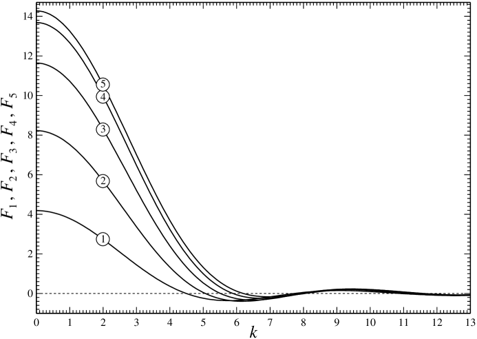
Figure 1: The functions $F_{l}(k)$ defined by (18). The curves are marked with the corresponding value of $l$.

Equality (17) is, essentially, an instability criterion: if a value of $k$ exists such that (17) is satisfied for a state $\left(n,T\right)$, this state is unstable.

4 The results

In what follows, we shall illustrate criterion (17) using the values for the coefficients $c_{l}$, obtained in [BenilovBenilov19] for noble gases. The series representing $Q$ was truncated at $L=5$, and

$$c_{2} =-1.3207,\hskip 30.44466ptc_{3}=9.9308,$$ (20)

$$c_{4} =-18.7526,\qquad c_{5}=13.1406,$$ (21)

As seen later, the shape of the Vlasov potential is of little importance, so we assume, on a more or less ad hoc basis,

$$\hat{\Phi}(k)=-\frac{1}{1+\left(Rk\right)^{4}},$$ (22)

where $R$ is, physically, the ratio of the spatial scale of the van der Waals force to the molecule’s size. Evidently, expression (22) complies with restriction (19).

The stability criterion (17), (20)–(22) describes a one-parameter family of curves $T=T(n)$ with $k$ being the parameter. The behavior of these curves depends on whether or not the fifth-order polynomial in $n$ in the denominator of (17) has positive roots. Computations show that no more than one such root exists, and it (dis)appear only if $F_{5}(k)\$changes sign – which it does do for infinite sequence of values of $k$ tending to infinity (see figure 1). Denoting these values by $k_{1}$, $k_{2}$, $k_{3}$…, we have computed

$$k_{1}\approx 6.2042,\qquad k_{2}\approx 8.0354,\qquad k_{3}\approx 11.6014.$$

A straightforward analysis of expression (17) shows that, in the range

$$0<k<k_{1},$$ (23)

the denominator of expression (17) does not have positive roots. As a result – and due to quick decay of $\hat{\Phi}(k)$ as $k$ increases – the curves $T(n)$ ‘recede’ within range (23) – see figure 2. Thus, the curve with $k=0$ determines the boundary of an instability region, which will be referred to as IR1.

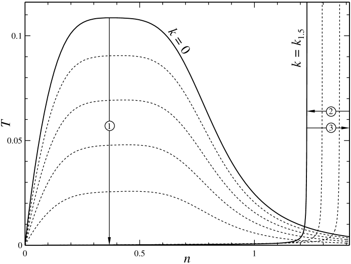
Figure 2: Existence of frozen waves on the $\left(n,T\right)$ plane. The curves $T(n)$ are determined by (17), (20)–(22) with $R=1$. Dotted curves within ranges (1)–(3) correspond to $k$ being within ranges (23)–(25), respectively. The boundaries of the instability regions are shown by solid lines.

Another instability region (IR2) arises for the range $k_{1}<k<k_{2}$ – which can be conveniently subdivided into two subranges,

$$k_{1}<k<k_{1.5},$$ (24)

with $k_{1.5}\approx 7.129$, and

$$k_{1.5}<k<k_{2}.$$ (25)

As $k$ changes from $k_{1}$ to $k_{1.5}$, the (real positive) root $n_{0}$ of the denominator of (17) ‘travels’ from $+\infty$ to $n_{0}\approx 1.230$. Then, when $k$ changes from $k_{1.5}$ to $k_{2}$, $n_{0}$ travels back to $+\infty$ – i.e., the boundary of IR2 corresponds to $k=k_{1.5}$. The corresponding curve $T(n)$ is shown in figure 2 together with examples of curves for $k$ from ranges (24) and (25).

A basic analysis of expression (17) and computations show that the instability regions corresponding to $\left(k_{2},k_{3}\right)$, $\left(k_{3},k_{4}\right)$, etc. are all inside IR1 and IR2 and, thus, are physically unimportant.

Finally, if $n\ll 1$ (diluted gas), the stability criterion (17) agrees with the corresponding results obtained in [BenilovBenilov16, BenilovBenilov17] for the BGK–Vlasov and Boltzmann–Vlasov models, respectively.

5 Discussion

For $k=0$ (the boundary of IR1), (17) and (19) reduce to

$$T=\frac{n}{1+\frac{4\pi}{3}nA_{1}+{\displaystyle\sum\limits_{l=2}^{L}}c_{l}n^{l}A_{l}},$$

where constants $A_{l}$ are given by (11). The above expression can be rewritten in terms of the function $\Theta(n)$ [given by (10)],

$$T=\frac{n}{1+\left[n^{2}\Theta^{\prime}(n)\right]^{\prime}}.$$ (26)

This representation of the boundary of IR1 turns out to be very useful.

(1) Equation (26) implies that IR1 does not depend on the specific shape of the Vlasov potential $\Phi$.

(2) As for IR2, it does depend on $\Phi$, but this dependence is weak – which we illustrate by computing the boundary of IR2 for different values of the parameter $R$ [which appears in expression (22)] and plotting the results in figure 3. One can see that, for $R\gtrsim 2$, the boundary of IR2 is virtually indistinguishable from a vertical line. This effect is even more pronounced if $\hat{\Phi}(k)$ decays exponentially as $k\rightarrow\infty$.

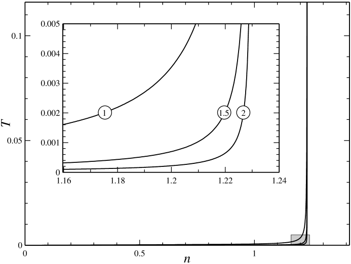
Figure 3: The dependence of the boundary of IR2 on the parameter $R$ of the Fourier transform (22) of the Vlasov potential. The inset shows a blow-up of the shaded region of the main panel. The curves are marked with the corresponding values of $R$.

Given that the van der Waals force is supposed to be long-range (by comparison with the molecule size), one can assume that $R\gg 1$, and thus replace the boundary of IR2 by a vertical line. Physically, this means that a fluid cannot be compressed beyond a certain density value no matter what the temperature is.

(3) Using EoS (12), one can show that the maximum of the function $T(n)$ given by (26) corresponds to the critical point.

(4) Not all of the stable states are physically meaningful, as some of them correspond to negative pressure. These can be detected using EoS (12). For the case (20)–(22) with $R=1$, the full diagram of stable and physically meaningful fluid states is shown in figure 4.

Figure 4: The stable, physically meaningful fluid states in the $\left(n,T\right)$ parameter plane. IR1 and IR2 stand for instability regions 1 and 2, respectively. The black dot marks the critical point.

(5) As stated in most thermodynamics texts, a non-ideal gas becomes unstable if

$$\left(\frac{\partial p}{\partial n}\right)_{T=\mathrm{const}}<0,$$ (27)

i.e., if an increase of density gives rise to a decrease of pressure. Applying this argument to EoS (12), we recover equation (26) describing the boundary of IR1.

IR2, in turn, is located in high-density region – hence, it may only describe fluid-solid transitions. Most importantly, the whole boundary of IR2 corresponds to a single value of the perturbation wavenumber, $k_{1.5}$ – so that $2\pi/k_{1.5}$ can be identified with the spatial scale of the emerging crystal. This agrees with the fact that that crystal structure does not depend on the temperature or density of the fluid state where the transition takes place.

(6) It is well-known that gas-liquid transition typically occurs before criterion (27) predicts it. The threshold where the actual transition occurs is determined by the so-called evaporation curve describing the gas-liquid equilibrium. It is still possible, however, to overcool a gas or overheat a liquid beyond this threshold, provided they are sufficiently pure. Thus, the boundaries of the instability regions are essentially the limits to which one can overcool or overheat a fluid before phase transition occurs.

To illustrate this interpretation, we have redrawn figure 4 on the $\left(T,p\right)$ plane, thus turning it into a phase diagram – see figure 5. We have also added empirically-derived evaporation, melting, and sublimation curves (the last two describe the solid-liquid and solid-gas equilibria, respectively).

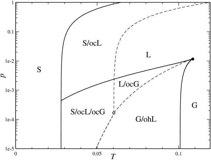
Figure 5: The phase diagram for argon in the nondimensional $\left(T,p\right)$ plane. Solid lines correspond to the boundaries of the instability regions computed using the EV model; dashed lines show the empiric evaporation, melting, and sublimation curves [TegelerSpanWagner99]. The critical and triple points are marked by a black dot and small circle, respectively. “G”, “L”, and “S” mark the regions where gas, liquid, and solid may exist; the prefixes “oc” and “oh” mean “overcooled” and “overheated”.

The following features of figure 5 can be observed:

• There are two single-phase regions: in the one marked “S”, only solid phase exists – and in the one whose parts are marked “L” or “G”, one of the two fluid phases exists (gas and liquid are difficult to separate in the latter case, as they can be continuously transformed one into another).

• In the transitional zone marked “S/ocL”, either solid or overcooled liquid can exist – and in the zone “S/ocL/ocG”, it is either solid or overcooled liquid, or overcooled gas.

• In the remaining two zones, “L/ocG” and “G/ohL”, either of the two fluid phases can exist.

6 Concluding remarks

In this work, we have used the Enskog–Vlasov model to examine when fluids are unstable, and with respect to which perturbations. The parameter range of the instability is illustrated in figure 4 on the nondimensional $\left(n,T\right)$ plane, and in figure 5, on the $\left(T,p\right)$ plane. These figures are the main results of this work.

Note that, in figure 5, we have calculated only the solid curves, whereas the dashed ones have been obtained by methods of statistical thermodynamics [TegelerSpanWagner99]. This does not mean that the EV model cannot be used to calculate the latter: in fact, it has been used for calculating the evaporation curve, producing a result with an error of only several percent [BenilovBenilov19]. Before calculating the melting and sublimation curves, however, one should explore periodic solutions of the EV equation which describe the solid (crystal) state; these solutions bifurcate from the spatially uniform (fluid) solutions as frozen waves. That is, we do not claim that the EV model can describe the fundamental physics of the solid state – but we do hope that it can ‘mimic’ it given a suitable choice of the functional $Q[n]$ and the Vlasov potential $\Phi$. In fact, the Enskog approach to dense fluids has been successfully used for describing hard-sphere crystals [Kirkpatrick89, KirkpatrickDasErnstPiasecki90] and studying equilibrium properties of the liquid–solid phase transitions [RamakrishnanYussouff79, HaymetOxtoby81] (for recent developments in the latter theory, see [Archer09, Lutsko12, BaskaranBaskaranLowengrub14, HeinonenAchimKosterlitzYingEtAl16]).

Once the EV model is calibrated to deal with all three phases, it would become an invaluable tool for modeling complex physical problems (e.g., evolution of liquid films with evaporation and solidification). This is an important point, as several version of the Enskog–Vlasov kinetic equation have been used for applications (see [FrezzottiBarbante17, FrezzottiGibelliLockerbySprittles18] and references therein).