Machine Learning as a universal tool for quantitative investigations
of phase transitions

Abstract

The problem of identifying the phase of a given system for a certain value of the temperature can be reformulated as a classification problem in Machine Learning. Taking as a prototype the Ising model and using the Support Vector Machine as a tool to classify Monte Carlo generated configurations, we show that the critical region of the system can be clearly identified and the symmetry that drives the transition can be reconstructed from the performance of the learning process. The role of the discrete symmetry of the system in obtaining this result is discussed. A finite size analysis of the learned Support Vector Machine decision function allows us to determine the critical temperature and critical exponents with a precision that is comparable to that of the most efficient numerical approaches relying on a known Hamiltonian description of the system. For the determination of the critical temperature and of the critical exponent connected with the divergence of the correlation length, other than the availability of a range of temperatures having information on both phases, the method we propose does not rest on any physical input on the system, and in particular is agnostic to its Hamiltonian, its symmetry properties and its order parameter. Hence, our investigation provides a first significant step in the direction of devising robust tools for quantitative analyses of phase transitions in cases in which an order parameter is not known.

1 Introduction

Phase transitions (a basic overview of which can be found e.g. in [1]) are ubiquitous phenomena in Statistical Mechanics, Condensed Matter and Particle Physics systems. In addition, applications of the physical concepts related to phase transitions have been proved successful in investigating problems in other scientific domains such as the boolean satisfiability problem in Mathematics (which is an archetypal example of an NP-complete problem, see e.g. [2]) and cancer dynamics. Some applications beyond traditional physical systems are discussed for instance in [3].

We say that we are in the presence of a phase transition when there is a point or an hypersurface in parameter space that separates two regions of the system with very different properties (e.g. the density of ice is significantly different from that of water, and this change happens at the freezing point). Mathematically, a phase transition is a singularity in physical observables as the number of degrees of freedom of the system goes to infinity. Understanding the dynamics of the two phases near the transition point and being able to quantify the location of the latter (in addition to establishing the presence of a transition, a question that sometimes has not an immediate answer) are wide reaching issues that have been investigated from various angles and perspectives since the early days of thermal physics, with invaluable insights that have originated some of the most remarkable ideas in theoretical physics. Two related examples of transformative ideas originating from the investigation of phase transitions are the concept of the renormalisation group and the deep connection between the concept of criticality in Statistical Mechanics and renormalisability of gauge theories [4].

The current standard approach to phase transitions relies on a first principle knowledge of the system. Generally, one investigates a system whose classical or quantum dynamics is in principle known and can be worked out from an explicit Hamiltonian or a Lagrangian, respectively. The Hamiltonian (Lagrangian) has some manifest symmetry that is spontaneously broken as a function of some control parameters. Based on this, one builds an order parameter, i.e. an observable that is not invariant under the relevant symmetry of the Hamiltonian (Lagrangian). In the phase in which the symmetry is implemented à la Wigner, the lack of invariance of the order parameter forces this observable to be zero. Conversely, the fact that the order parameter observable is different from zero in a phase is an explicit signal that in that phase the symmetry is not linearly realised, i.e. one is in the presence of a spontaneously broken symmetry. A system in which the symmetry is spontaneously broken possesses a set of degenerate groundstates that transform into each other under the relevant symmetry group rather than a single, symmetric groundstate, as it is the case in the symmetric phase.

This ab initio approach, which is by now consolidated and described in detail in various textbooks (e.g. [5]), has produced widely accurate results in a variety of contexts, including Monte Carlo simulations of gauge theories (see [6] for a recent example). However, there are relevant physical systems for which the order parameter is hard to identify and currently unknown, mainly because the symmetry that drives the phase transition is not manifest in the Hamiltonian. Remarkable examples in this class are topological phases [7], in which the phase transition, being of a topological nature, is driven by a dual order parameter that might not be immediate to express in terms of the local variables or indeed might not be known in terms of the latter, and Quantum Chromodynamics (the theory of the strong force) at finite quark mass, for which it is still debated what is the mechanism that drives the phase transition (when it exists, as a function of the constituent quark mass) and whether it is possibly of a topological nature (e.g. [8].)

Recently, a surge of interest has been generated by the possibility of using Machine Learning inspired techniques for identifying phase transitions [9]. The underlying idea is to use clustering techniques to identify properties of the phase transitions without any a priori information (a setup that in the Machine Learning terminology is referred to as unsupervised learning) or by using particular realisations of the system for which the phase is known unambiguously to understand whether there is a critical set of parameters for which the phase transition takes place (supervised learning). Both supervised and unsupervised learning characterisations of phase transitions have produced encouraging first results for identifying and studying phase transitions in Condensed Matter, Statistical Mechanics and Quantum Field Theory. An incomplete set of references is provided by [9, 10, 11, 12, 13, 14, 15, 16, 17, 18, 19, 20, 21, 22, 23, 24, 25, 26, 27, 28, 29, 30, 31, 32, 33, 34], with a recent review given in [35].

To our knowledge, so far all studies have focused on qualitative and semi-quantitative results using a varying degree of a priori knowledge on the target system. In this paper, we shall investigate whether it is possible to identify the critical region and characterise it from a quantitative point of view by using Machine Learning with a minimal number of assumptions. To be more specific, we will ask whether from the simple knowledge of states of the system at various temperatures we can predict whether a phase transition takes place and in case extract precise values of observables and critical quantities such as the critical temperature and critical exponents as the system undergoes the transition. As the system of choice for this analysis we have taken the Ising model in two dimensions, which has an exact analytical solution and can be investigated numerically with efficient Monte Carlo techniques. From the Machine Learning point of view, we do the investigation with a Support Vector Machine (SVM) analysis of Monte Carlo generated data. This will be contrasted to a traditional analysis of the same Monte Carlo data. One of the characteristics of the SVM that makes it particularly suitable for investigating quantitative issues is that its predictions are based on controlled analytical models whose parameters are extracted with well-defined optimisation procedures. Once the model reconstructed by the algorithm on the data is known, in principle one can use it to get insights on the physical phenomenon that drives the transition. Among recent studies of phase transitions with Machine Learning techniques, our work share a similar approach with [13]. However, there are significant differences between our investigation and the latter reference (for instance, the training strategy), on which we shall return later. The main findings of our study are: (a) for the Ising model, the critical region is easily identified by training the SVM with two ensembles of 200 configurations, each obtained at temperature values that are respectively one deep in the ordered phase, the other deep in the disordered phase; (b) information on the symmetry and on the optimal training temperatures can be obtained by optimising the performance of the learned model, the physical case corresponding to the best performance; (c) once the algorithm has been optimised, a finite size scaling analysis of the classification function (called the decision function for the SVM) yields results for the critical temperature and for the critical exponents that are comparable in precision to those obtained from finite size scaling of an a priori known order parameter, even if we have not informed the process with any previous knowledge on the underlying physics driving the phase transition.

The rest of the paper is organised as follows. The formulation of the Ising model and the description of its critical properties are the subject of Sect. 2, where we also discuss the Monte Carlo method for generating the data that we have processed with the SVM. In Sect. 3 we review the mathematical framework underpinning the SVM, with emphasis on the aspects that have been used in our work. Our numerical analysis using the SVM will be reported in detail in Sect. 4. Finally, our findings are summarised in Sect. 5, where we also outline potential future directions.

2 The phase transition of the Ising model

Due to the simplicity of its formulation coupled to the non-trivial features it displays, the Ising model is commonly used to illustrate key concepts and test new techniques in Statistical Mechanics. Its most direct physical counterpart is a ferromagnet in the vicinity of the Curie point, but the model can also be reformulated to describe a lattice gas or a binary alloy. More in general, the Ising model describes an order-disorder phase transition in dimension two and above. In two dimensions, it can be solved analytically in a physically relevant region of parameter space. It is both the presence of a non-trivial phase structure and the availability of an analytical solution that make the Ising model in two dimensions an ideal test bed for new approaches and ideas in Statistical Mechanics, Condensed Matter and Lattice Field Theory. In this work, we shall use the model to explore whether a quantitative study of the phase transition (more specifically, critical temperature and critical exponents) can be performed using Machine Learning methods. In order to provide a comparison of these techniques with a more traditional Monte Carlo approach, in this section we present a study with the latter method.

The Ising model is defined by the Hamiltonian

$$\mathcal{H}=-\mathcal{J}\sum_{\langle i,j\rangle}\sigma_{i}\sigma_{j}-h\sum_{i}\sigma_{i}~{},$$ (1)

with the $\sigma$’s, which take the values $\pm 1$, being conventionally referred as spins. Each spin is defined on the sites of a two dimensional lattice that we take to be a squared grid with equal spacings in the two orthogonal directions and closed with periodic boundary conditions. Each side of the lattice has total length $L$ and the total area occupied by the system is given by $V=L^{2}$. $\sum_{\langle i,j\rangle}$ indicates a sum over nearest neighbours. $\mathcal{J}$ is the nearest-neighbour spin-spin coupling (that we choose ferromagnetic, i.e. $\mathcal{J}>0$). $h$ is an externally applied field (in the traditional ferromagnetic language, which we follow from now on, $h$ is an external magnetic field), coupled linearly with each spin.

At vanishing external magnetic field, the state of lowest (internal) energy is easily seen to be an ordered state, in which all of the $\sigma$’s have the same value, $+1$ or $-1$. A non-zero value of $h$ splits the degeneracy of those two states, with the ground state having all spins aligned to $h$. At finite temperature $T=1/(k\beta)$, with $k$ the Boltzmann constant, the probability of finding the system in a configuration with spins taking the values $\{\sigma_{i}\}$ is given by

$$p(\{\sigma_{i}\})=\frac{1}{Z}~{}e^{-\beta\mathcal{H}}\ ,$$ (2)

where $Z$ is the partition function

$$Z(\beta,h)=\sum_{\left\{\sigma_{i}=\pm 1\right\}}e^{-\beta\mathcal{H}}=e^{-\beta F}\ ,$$ (3)

with $F$ the free energy of the system. The sum defining $Z$ is taken over all possible values of the spins. For later use, we define the ensemble average of an observable $O$ depending on the spin variables $\sigma_{i}$ as

$$\langle O\left(\left\{\sigma_{i}\right\}\right)\rangle=\frac{1}{Z}\sum_{\left\{\sigma_{i}=\pm 1\right\}}O\left(\left\{\sigma_{i}\right\}\right)e^{-\beta\mathcal{H}}\ .$$ (4)

Let us now consider for simplicity the case $h=0$. Due to the fact that the weights $e^{-\beta\mathcal{H}}/Z$ are positive definite for any realisation of the spin configuration $\left\{\sigma_{i}=\pm 1\right\}$, the expression defining $O$ has a simple interpretation as the average over the probability distribution provided by the normalised Boltzmann factor

$$P(\mathcal{H}=E)=\rho(E)e^{-\beta E}/Z\ ,$$ (5)

where the function $\rho(E)$, which counts the number of configurations giving $\mathcal{H}=E$, is known as the density of states. In terms of $\rho(E)$ we can rewrite

$$Z(\beta)=\sum_{E}\rho(E)e^{-\beta E}\ .$$ (6)

For low temperatures (corresponding to large $\beta$), we expect the Ising system to have a significant number of spins pointing to the same direction. While this direction is arbitrary, the dynamics will force the system to choose one, and tunnelling between the two will be exponentially suppressed with the size of the system. The dynamical selection of a particular state, out of a set of symmetrically connected ones with the same energy, realises the key concept of spontaneous symmetry breaking. In our model, the Hamiltonian $\mathcal{H}$ is invariant under the simultaneous transformation of all the spins

$$\sigma_{i}\mapsto-\sigma_{i}\ ,$$ (7)

which is implemented by the (global) symmetry group $\mathbb{Z}_{2}\equiv\{-1,1\}$. A $\mathbb{Z}_{2}$ transformation, however, does not leave invariant the two degenerate groundstates, but interchanges them. For this reason, the choice of a groundstate (or more in general of a preferred direction of spin alignment) over the other breaks the invariance of the system. The expression spontaneous symmetry breaking underlines the crucial fact that the global symmetry of the Hamiltonian is broken by the dynamics rather than by some explicit coupling.

In the opposite limit of very high temperature, the energy component of the free energy of the system becomes negligible if compared to the entropy term. In this regime, spins are effectively randomised, with no clear alignment being visible. In this phase, the $\mathbb{Z}_{2}$ symmetry of the system is restored. The phase with spontaneously broken symmetry is separated from the symmetric phase by the critical value of the temperature $T_{c}$ given by

$$kT_{c}=2{\cal J}/\left(k\log\left(1+\sqrt{2}\right)\right)\ .$$ (8)

In general, a quantity that allows us to distinguish in which phase we are is called an order parameter. The order parameter of the Ising model is the reduced magnetisation $m=M/V=\langle\sum_{i}\sigma_{i}/V\rangle$ ($M=\langle\sum_{i}\sigma_{i}\rangle$ is called the total magnetisation) . For this observable, in the limit $L\to\infty$, one finds

$$|m|=\big{|}\langle\sum_{i}\sigma_{i}\rangle\big{|}/V=\begin{cases}=0&\mbox{$\beta<\beta_{c}$,}\\ \neq 0&\mbox{$\beta>\beta_{c}$~{}.}\end{cases}$$ (9)

Another important quantity is the correlation length $\xi$, which can be understood as the range of the effective interactions or, equivalently, the typical size of a region (cluster) over which spins are aligned. $\xi$ is formally defined from the expected scaling of the correlation of two spins $\sigma_{l}$ and $\sigma_{m}$ sitting at points $l$ and $m$ as

$$\langle\sigma_{l}\sigma_{m}\rangle-\langle\sigma_{l}\rangle\langle\sigma_{m}\rangle\ \mathop{\sim}^{r\to\infty}\ \frac{e^{-r/\xi}}{r^{p}}\ ,$$ (10)

where $r$ is the distance between $l$ and $m$. $p$ is a calculable exponent that near the critical temperature is given by

$$p=d-2+\eta\ ,$$ (11)

where $d$ is the dimension of the system ($d=2$ in our case) and $\eta$ is a dynamical exponent called anomalous dimension.

As the critical point is approached, clusters grow in size and, exactly at the critical temperature, clusters of all sizes are present. At this point, the system is invariant with respect to a scale transformation and the correlation length is infinite. The divergence of $\xi$ as $t\to 0$ is observed to behave as a power law, i.e.

$$\xi\propto|t|^{-\nu}~{},$$ (12)

where $t=(T_{c}-T)/T_{c}$ is called the reduced temperature and $\nu$ is the thermal critical exponent.

Other thermodynamic quantities sensitive to the phase transition like the magnetisation $m$ and the magnetic susceptibility $\chi=V\left(\langle\sum_{i,j}\sigma_{i}\sigma_{j}\rangle/V^{2}-m^{2}\right)$ have power-low singularities as $T_{c}$ is approached:

$$|m|\mathop{\propto}_{t\to 0^{+}}t^{\beta}\ ,\qquad\chi\mathop{\propto}_{t\to 0}t^{-\gamma}\ ,$$ (13)

where $\beta$ and $\gamma$ are two additional (calculable in our case) critical exponents.

The final two phenomenologically relevant critical exponents, $\delta$ and $\alpha$, are defined from the following behaviours:

$$\big{|}m\big{|}_{t=0}\propto|h|^{1/\delta}\ ;$$ (14)

$$c_{V}=\frac{1}{V}\left(\langle H^{2}\rangle-\langle H\rangle^{2}\right)\propto t^{-\alpha}\ ,$$ (15)

$c_{V}$ being the specific heat of the system.

The power law behaviour of the above or similarly defined quantities (and hence the existence of critical exponents) is a general feature of second order phase transitions, and not only a characteristic of the Ising model. Hence, an essential aspect of any study (numerical or analytical) of a phase transition is the derivation of its critical exponents. The importance of these quantities is highlighted by the phenomenon of universality: systems with very different interactions, but with the same symmetry structure and having the same dimensionality, share the same critical behaviour. Therefore, rather than being specific to the model, the set of critical exponents $(\alpha,\beta,\gamma,\delta,\nu,\eta)$ only depend on the dimensionality of the system and on the symmetry of its Hamiltonian, and not on the microscopic structure of the latter. Universality makes the Ising model very relevant for studies of systems with more complicated Hamiltonians that display the same global $\mathbb{Z}_{2}$ symmetry.

Using the scaling hypothesis, which assumes that the free energy is an homogeneous function of $t$ and $h$ with respect to rescaling of lengths by an arbitrary factor of $b$, one can derive the following scaling relations:

$$\begin{array}[]{l l}\text{Fisher Law:}&\gamma=\nu(2-\eta)\ ,\\ \text{Widom Law:}&\gamma=\beta(\delta-1)\ ,\\ \text{Rushbrooke Law:}&\alpha+2\beta+\gamma=2\ ,\\ \text{Josephson Law:}&\nu d=2-\alpha\ ,\end{array}$$ (20)

which show that only two of the critical exponents are independent, while the others can be derived. The two critical exponents that are directly related to the rescaling of $t$ and $h$ are respectively $\nu$ and $\eta$. Hence, based on this physical motivation, these two exponents are considered fundamental, while the others are considered secondary.

While in the specific case of the two-dimensional Ising model the availability of an explicit solution allows us to compute the critical exponents and the critical temperature, in more general settings one has to resort to first-principle numerical techniques. In a Monte Carlo based numerical approach, two aspects would need to be considered: (i) the generation of a sample of configurations of the system according to the Boltzmann weight Eq. (5), in order to compute observables in a controlled way; and (ii) the extraction of critical exponents from the scaling of key observables with the size of the system.

For the first step above, a Markovian process is defined that allows one to obtain a chain of configurations distributed according to the Boltzmann weight computed at the target temperature. The physics of the system plays a crucial role in designing an efficient Markov process. In the case of the Ising model, the Wolff algorithm [36] provides the most suitable method for exploring the configuration space. According to this algorithm, in order to generate a configuration from a preceding one, we start from a randomly chosen spin, called seed, from which a cluster is grown by adding to it neighbour spins with the same orientation with probability $1-e^{-2\beta\mathcal{J}}$. The growth process proceeds by exploring the neighbourhood of the newly added spins and applying the same growth rule until all equally oriented spins connected to the seed have been proposed for addition, at which point the whole cluster is flipped. This process defines a new configuration that becomes the next element of the Markov chain. If one starts from a random configuration, general principles of Markov processes guarantee the convergence to the equilibrium distribution given by (5). With a chain of $N$ thermalised configurations $C_{j}$, the thermal average of an observable $O$ can be written as

$$\langle O\rangle\simeq\sum_{j}O(C_{j})e^{-\beta H(C_{j})}/\left(\sum_{j}e^{-\beta H(C_{j})}\right)\ ,$$ (21)

where the convergence of the approximated value to the exact one is ${\cal O}(1/\sqrt{N})$. Since the latter is a statistical controllable error, the method is first principles, in the sense that there is a rigorous way for approximating the exact result at any specified level of precision. While this is a general fact, we remark for completeness that in practical applications of Monte Carlo methods systematic errors may arise. The most common ones are due to thermalisation (i.e. if not enough configurations are discarded before the Markov process reaches the stationary distribution), autocorrelation (characterised as lack of enough information in the sample due to slow dynamics of the Markov process) and lack of ergodic exploration of the configuration space (due, e.g., to the presence of disconnected topological sectors). The systematics is well under control in the two-dimensional Ising model, thanks to the availability of efficient algorithms that have been tested against the known solution. Powerful general tests also exist for systems where an analytic solution is not known, although these tests (often based on comparisons with semi-analytic or perturbative approaches) are only as good as our prior knowledge of the broad physical properties of the system.

In general, the values of the critical exponents can be obtained from the use of finite size scaling, whereby the size of the system $L$ enters scale-invariance arguments as a renormalisation group relevant quantity with length dimension one. Given that one can build the adimensional ratio $\xi/L$, we can trade the correlation length $\xi$ with $L$, which does not introduce new scaling exponents. Under the assumption that the finite volume corrections to scaling are analytic in $\xi/L$, one can derive the textbook relation

$$\beta_{c}-\beta_{c}(L)\propto L^{-1/\nu}\ ,$$ (22)

where $\beta_{c}(L)=(T_{c}(L))^{-1}$ is the value at which a susceptibility such as $\chi$ computed at volume $V=L^{2}$ achieves its maximum. This maximum value, which will be referred to as $\chi_{\text{max}}$, diverges as $L\to\infty$, with its position converging to $\beta_{c}$. Using scaling arguments, one can show that

$$\chi_{\text{max}}\propto L^{\gamma/\nu}\ .$$ (23)

The whole set of critical exponents can be reconstructed by measuring the value of $\chi_{\text{max}}(L)$ and of its position $\beta_{c}(L)$ and using the asymptotic behaviours provided in Eqs. (22,23) to determine $\nu$ and $\gamma$. In practical applications, these exponents are extracted through a fit on a set of data obtained at different volumes. In this process, one has to consider that these arguments are asymptotic. A systematic error can henceforth arise if the volumes explored are not in the asymptotic region. This error is generally controlled by repeating the analysis discarding smaller volumes and adding larger ones, until a regime of convergence is determined. In the Ising case, one can cross-check the results against the analytic solutions. When an analytic solution is not available, comparisons with other approaches (e.g. predictions in a $4-\epsilon$ expansion, when the latter is sufficiently reliable) can be instructive. Another source of systematic errors come from scaling violations, which, however, general arguments show to be sub-leading and undetectable at the level of precision that can be reached in standard simulations, their identification requiring dedicated methodologies. Hence, we neglect them for the remainder of our discussion.

Using conventional analysis of Monte Carlo simulated data based on scaling arguments, we extracted numerically the critical temperature and the critical exponents of the model, comparing our determination to the known exact results. We stress that this approach is very well established and has been used for the study of phase transitions in various Condensed Matter, Statistical Mechanics and Field Theory models (including the Ising model) for a long time. The reason why we repropose it here is to be able to assess the quality of our SVM analysis, comparing the results on the same set of input data.

Our Monte Carlo simulations were run on $L^{2}$ lattices of linear size ranging from $L=32$ to $L=1024$ and for several values of temperatures between $T=0.5$ and $T=5.0$. Near the transition, $3000$ Wolff clusters were flipped for thermalisation, in order to allow the system to relax to its equilibrium state, and the configurations were recorded once every $15$ Wolff updates. Far from the transition, the separation between configurations was reduced, as temporal correlations of the Markov chain are less severe. For each lattice size and temperature value, we recorded $200$ configurations. For the scaling analysis that allowed us to extract $\beta_{c}$, $\nu$ and $\gamma$ we used data for order $20$ equally spaced temperature values $T$ in the critical region, i.e. in a small neighbourhood of $T_{c}$ in which one can verify a posteriori that scaling arguments apply. The simulated values are reported in Tab. 1.

$L$	$T_{\text{min}}$	$T_{\text{max}}$	$n_{\text{steps}}$
$64$	$2.280$	$2.330$	$20$
$128$	$2.275$	$2.294$	$20$
$240$	$2.273$	$2.285$	$24$
$360$	$2.270$	$2.280$	$20$
$440$	$2.270$	$2.280$	$20$
$512$	$2.2665$	$2.2770$	$22$
$760$	$2.27000$	$2.27400$	$20$
$1024$	$2.27000$	$2.27300$	$30$

$L$	$T_{c}$	$\chi_{\text{max}}$
$64$	$2.3037(29)$	$1.284(37)\cdot 10^{2}$
$128$	$2.28664(74)$	$4.590(97)\cdot 10^{2}$
$360$	$2.27528(28)$	$2.781(65)\cdot 10^{2}$
$440$	$2.27448(47)$	$3.97(10)\cdot 10^{3}$
$512$	$2.27351(29)$	$5.24(14)\cdot 10^{3}$
$240$	$2.27892(39)$	$1.383(28)\cdot 10^{3}$
$760$	$2.27226(25)$	$1.035(21)\cdot 10^{4}$
$1024$	$2.27145(23)$	$1.757(40)\cdot 10^{4}$

Table 1: On the left, scanning windows of temperatures for extracting the pseudocritical temperature $T_{c}(L)$ at each value of $L$; $n_{\text{steps}}$ indicates the number of simulated values of $T$, all equally spaced between the two extremes $T_{\text{min}}$ and $T_{\text{max}}$. On the right, values of the pseudocritical temperature $T_{c}$ and the corresponding maximum of the magnetic susceptibility, as obtained from the multi-histogram method.

To extract the infinite volume critical coupling and the critical exponents $\nu$ and $\gamma/\nu$, we fitted Eq. (22) and Eq. (23) to the data in the critical region using $\beta_{c}(\infty)\equiv\beta_{c}$, $\nu$ and $\gamma/\nu$ as fitting parameters after reweighting the measured observables with the multi-histogram method (see Appendix A.1). Errors were estimated using bootstrap (described in Appendix A.2). The results can be found in the first row of Tab. 2. In the same table, the second row reports fits in which the values of the critical exponents are fixed to their analytically computed values. The fit results are visible in Fig. 1.

As expected, the method reproduces well the analytically computable results, with a precision of order $10^{-4}$ on $T_{c}$, and of $10^{-3}$ on $\gamma/\nu$ (with the central value in this latter case being compatible with the expected value within two standard deviations, while in the former the compatibility is within the statistical error). The critical exponent $\nu$ is determined with a precision of the order of five percent. More precise results can be obtained by increasing the number of generated configurations and/or the set of simulated temperatures, which in this model can be achieved with a moderate increase in computational time. However, we stress that the purpose of the study we have discussed is to establish a numerical benchmark for the SVM analysis provided in Sect. 4 using the same input information, rather than performing a high precision investigation of the phase transition in the Ising model with finite size scaling techniques, which is by now a classic topic in specialised textbooks (see e.g. [37]).

$T_{c}$	$\nu$	$\chi^{2}_{r}$	$\gamma/\nu$	$\chi^{2}_{r}$
$2.26922(33)$	$1.004(48)$	$0.36$	$1.7634(68)$	$0.46$
$2.26925(11)$	$1$ (exact)	$0.3$	$7/4$ (exact)	$0.66$

Table 2: On the left, the extracted values of $T_{c}$ and $\nu$ obtained from fitting Eq. (22) to the data at the simulated values of $L$. On the right, the extracted values of $\gamma/\nu$ obtained from fitting Eq. (23) to the data. We also show $\chi^{2}_{r}$, the $\chi^{2}$ per degree of freedom, of each fit.

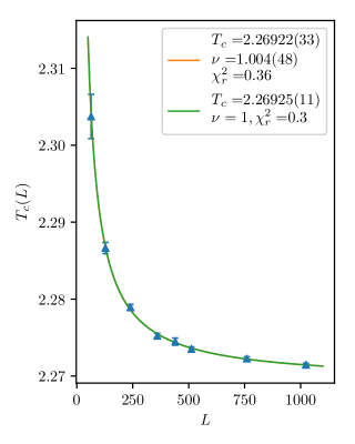
(a)

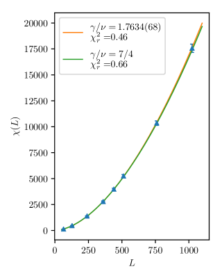
(b)

Figure 1: (Colour online) Left: behaviour of the pseudocritical temperature with the linear size of the lattice. Right: behaviour of the peak value of magnetic susceptibility with the linear size of the lattice. A fit to the expected asymptotic functional form is also displayed.

3 Ensemble classification and the Support Vector Machine

The Support Vector Machine (SVM) is a popular supervised learning algorithm used to solve classification and regression problems. In the field of Machine Learning, supervised learning approaches use labelled training data (i.e. data for which the classification is known) to find a model describing the functional relationship $Y=f(X)$ between a response variable $Y$ (where most often $Y$ is a label, i.e. a set of discrete values) and input variable(s) $X$. The learned model enables one to predict values of $Y$ for previously unseen values of $X$. Supervised learning is often contrasted to unsupervised learning approaches. The goal of unsupervised learning is to model the underlying structure of the data to discover patterns (for instance finding clusters of observations) and insightful representations rather than predicting a functional relationship. Unike in supervised learning, in this case the learning process uses only the input values $X$, assuming no knowledge of any output. Both supervised and unsupervised methods are widely used for modelling and prediction for a variety of applications including fraud detection, image and speech recognition, quality control and defect or failure prediction. In addition to SVM, supervised learning techniques include Artificial Neural Network, Decision Trees and K-Nearest Neighbour, while unsupervised learning can be achieved through clustering (k-means or EM Clustering), Kernel Density Estimation, Principal Component Analysis (PCA) and Self Organising Maps (SOM).

SVM was firstly introduced in 1963 by Vladimir Vapnik and Alexey Chervonenkis, and further developed in the 90’s as a general solution to linear binary and multi-class classification problems, and as the generalisation thereof to cases in which the target data are not linearly separable [38, 39]. The SVM method can also be modified to solve regression problems when the label can take continuous real values instead of categorical values. The SVM method is very effective in high dimensional spaces where the number of dimensions is greater than the number of samples (see e.g. [40]). It also differs from other supervised learning techniques such as Artificial Neural Network because it can be expressed as a convex optimisation problem and, if a solution exists, it is always found as the unique global minimum of the equivalent optimisation problem [41]. The simple visual interpretation of the procedure and the possibility to use a wide range of functional forms (provided by transformations that in this context are called kernels) make the SVM an effective method in problems when boundaries that separate the data (the decision boundaries) can not be expressed as a linear hyperplane in the space of the input variables [42].

In the most straightforward case, an SVM deals with a binary classification problem between linearly separable datasets. For this problem, in the space of the input variables, the SVM method seeks to find the maximum margin hyperplane separating data belonging to the two classes. Given $N$ linearly separable training points $(x_{i},y_{i})$, with $x_{i}\in\mathbb{R}^{d}$ and $y_{i}\in\{-1,1\}$, there are generally many possible separating hyperplanes, all specified in $d$-dimensional space by the equation

$$\vec{\omega}\cdot\vec{x}-\hat{\beta}=0,$$ (24)

for appropriate values of $\vec{\omega}$ and $\hat{\beta}$, with $\vec{\omega}$ the normal vector to the plane and $\hat{\beta}$ its offset with respect to the origin. For each of these hyperplanes, a margin can be defined as the region of space delimited by the two hyperplanes that are parallel to the separating hyperplane and pass through the closest data points that lie on either side of it. These points are called support vectors. For each support vector, we define the size as the distance between that support vector and the separating hyperplane. As the name suggests, a Support Vector Machine is an algorithm that seeks to find the maximum margin hyperplane, as determined by its support vectors. This plane is identified by the equation

$$\vec{w}\cdot\vec{x}-b=0\ ,$$ (25)

where $\vec{w}$ and $b$ are obtained through a maximisation process as discussed below. Once $\vec{w}$ and $b$ have been found, we are still free to rescale them such that

$$\vec{w}\cdot\vec{x}-b=1,\quad\vec{w}\cdot\vec{x}-b=-1$$ (26)

for the support vectors, where we fix the convention that the first equation holds for support vectors corresponding to label $+1$ and the other for those with label $-1$. The size of the margin (i.e. the maximum separating slab) will be $2/|\vec{w}|$ and for points $\left\{\vec{x}_{i},~{}y_{i}\right\}$ on either side of the maximal margin hyperplane, $y_{i}(\vec{w}\cdot\vec{x}_{i}-b)\geq 1$. A diagram that illustrates the linearly separable case is provided in Fig. 2, left.

Finding the maximum margin hyperplane can be reformulated mathematically as the minimisation problem

$$\min_{\vec{\omega},\hat{\beta}}||\vec{\omega}||^{2}\text{ s.t. }y_{i}(\vec{\omega}\cdot\vec{x}_{i}-\hat{\beta})\geq 1,~{}\forall i=1,\dots,N\ ,$$ (27)

where $N$ is the total number of training data. The solution of this problem delivers the values of $\vec{w}$ and $b$ that allow us to define the desired classifier

$$f(\vec{x})=\mathrm{sign}\left(\vec{w}\cdot\vec{x}-b\right)$$ (28)

assigning a value $\pm 1$ to any pervasively unseen $\vec{x}$ depending on whether it lays above or below the maximal separting hyperplane. The decision function is defined as

$$d(\vec{x})=\vec{w}\cdot\vec{x}-b$$ (29)

and its (signed) value determines the distance of $\vec{x}$ from the separating hyperplane.

We now proceed to generalise the above picture by relaxing the assumption of strict linear separability. We introduce the slack variables $\xi_{i}$ defined as

$$\xi_{i}=\max(~{}0,~{}1-y_{i}(\vec{w}\cdot\vec{x}_{i}-b)~{})~{}.$$ (30)

If the data are such that $\left\{\xi_{i}=0\right\}$, we fall back to the linearly separable case. When some of the $\xi_{i}$’s are non-vanishing, the corresponding data points fall into the margin. In that case, we associate a penalty $C$ to each of the non-vanishing $\xi_{i}$’s and we modify condition (27) as

$$\min_{\vec{\omega},\hat{\beta}}\left(||\vec{\omega}||^{2}+\frac{C}{N}\sum_{i=1}^{N}\xi_{i}\right)\ \text{ s.t. }\xi_{i}=\max(0,~{}1-y_{i}(\vec{\omega}\cdot\vec{x}_{i}-\hat{\beta}))~{}\forall i~{}.$$ (31)

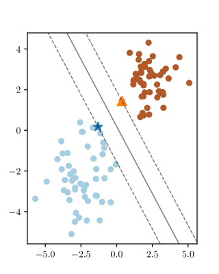
(a) Example of linearly separable data.

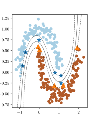
(b) Example of non-linearly separable data.

Figure 2: (Colour online) Two archetypal examples of distributions of training data in a two-class SVM classification problem, taken for simplicity to be bidimensional. Circles with the same shade indicate points in the same known class and each axis represents a feature. The separating hyperplane or hypersurface is denoted with a solid line and the margin on either side is indicated by a dashed line. The support vectors for each of the two classes are represented respectively with stars (corresponding to the lighter points) and with triangles (corresponding to the darker points).

For $C=0$, the unique solution to the minimisation problem can only be found in the linearly separable case, as a hard-margin classifier. For non vanishing $C$, the solution is called a soft-margin classifier. Using Lagrangian language, the problem is to minimise

$$L=\frac{1}{2}||\vec{\omega}||^{2}+\frac{C}{N}\sum_{i=1}^{N}\xi_{i}+\sum_{i=1}^{N}\alpha_{i}\left(1-y_{i}\left(\vec{\omega}\cdot\vec{x}_{i}-\hat{\beta}\right)-\xi_{i}\right)-\sum_{i=1}^{N}\eta_{i}\xi_{i}$$ (32)

with respect to $\vec{\omega},~{}\xi_{i},\hat{\beta}$, where $\alpha_{i}$ and $\eta_{i}$ are Lagrange multipliers. Note that, as requested by the Karush-Kuhn-Tucker conditions, $\alpha_{i},~{}\eta_{i}\geq 0$. Setting the gradients of $L$ to zero imposing

$$\delta_{\vec{\omega}}~{}L=0\ ,\qquad\delta_{\hat{\beta}}~{}L=0\ ,\qquad\delta_{\vec{\xi}}~{}L=0$$ (33)

yields

$$\vec{\omega}-\sum_{i=1}^{N}\alpha_{i}y_{i}\vec{x}_{i}=0\ ,\qquad\sum_{i=1}^{N}\alpha_{i}y_{i}=0\ ,\qquad\frac{C}{N}-\alpha_{i}-\eta_{i}=0\ .$$ (34)

Plugging these into the original Lagrangian, one obtains

$$L=-\frac{1}{2}\sum_{i,j=1}^{N}\alpha_{i}\alpha_{j}y_{i}y_{j}\vec{x}_{i}\cdot\vec{x}_{j}+\sum_{i=1}^{N}\alpha_{i}\ \text{s.t. }\sum_{i=1}^{N}\alpha_{i}y_{i}=0\text{ and }0\leq N\alpha_{i}\leq C\ ,$$ (35)

where now the extremisation would need to be performed over the $\alpha_{i}$. If the unique solution exists, we call $\{a_{i}\}$ the set of the $\alpha$’s that maximises $L$.

Eq. (35) expresses the dual formulation of the problem of finding the maximally separating hyperplane, which is the starting point to generalize the applicability of the method to cases where linear separation is not possible. Indeed, note that $L$ now only depends on the inner product between representative vectors of training samples. In cases in which the problem does not appear to have a solution in $\mathbb{R}^{d}$, we might seek one in another space of larger dimensionality. We can then consider a more general Lagrangian functional

$$\tilde{L}=\frac{1}{2}\sum_{i,j}y_{i}y_{j}\alpha_{i}\alpha_{j}\mathcal{K}(\vec{x}_{i},\vec{x}_{j})-\sum_{i=1}^{n}\alpha_{i}\ ,$$ (36)

where $\mathcal{K}(x_{i},x_{j})$ is referred to as a kernel. Note that in writing Eq. (36) we have multiplied the natural generalisation of (35) by a global $-1$, which means that, in order to follow the standard convention, we have rewritten our original maximisation problem into a minimisation problem. As it is transparent from Eq. (36), the value of the kernel computed on the input data is all the information that the minimisation algorithm sees. For this reason, the kernel is often denoted as an information bottleneck in this kind of analyses. Thus, the choice of kernel is crucial. Obviously, the kernel must be symmetric in its arguments, reflecting the symmetry under exchange of two training sets. If we require that the minimisation problem above has a unique global solution, then we must also require that $\mathcal{K}$ is positive definite (the optimisation problem is then convex). According to Mercer’s theorem, there exists then a map $\Phi:\vec{x}\to\Phi(\vec{x})$, called feature maps, such that the kernel can be represented as a dot product in some higher dimensional space, $\mathcal{K}(x_{i},x_{j})=\Phi(\vec{x}_{i})\cdot\Phi(\vec{x}_{j})$. Other than the conditions above, our choice of kernel must be guided by our knowledge of the system, performance or computational ease. If a solution is found that minimises $\tilde{L}$ in the image space for a given $\Phi$, we define the decision function as

$$d(\vec{x})=\sum_{i=1}^{N}\alpha_{i}y_{i}\Phi(\vec{x}_{i})\cdot\Phi(\vec{x})+b\ .$$ (37)

As in the linearly separable case, the sign of the decision function determines the predicted label of each input point. An illustrative representation of a non-linearly separable data set in the space of the input data (again, for this purpose assumed to be two-dimensional) is provided in Fig. 2, right.
The structure of a kernel that allows us to separate the training data is closely related to the dynamics of the system. Henceforth, the selection of a class of kernels embodies assumptions about the data to be analysed. The more these assumptions are constraining, the smaller is the class of functions among which we can choose our kernel. For a comprehensive and agnostic analysis, intuitively, we would be led to choose from a very large class of kernels, in order to reduce any bias due to any possible assumption. However, when we try and infer some physical behaviour from the ability of a kernel to separate the training set, this latter approach will generally reflect in a larger number of parameters that need to be optimised for the given data, with a correspondingly higher variance in the final result, notably due to fitting noise. There is therefore a trade-off between variance and bias that is central in many discussions in Machine Learning.
A set of kernels that will be important for analysis below is the class of polynomial kernels of degree $n$,

$$\mathcal{K}(\vec{x}_{i},\,\vec{x}_{j})=\left(\frac{\vec{x}_{i}\cdot\vec{x}_{j}}{\Gamma}+c_{0}\right)^{n}=\sum_{a=0}^{n}\binom{n}{a}c_{0}^{n-a}\left(\frac{\vec{x}_{i}\cdot\vec{x}_{j}}{\Gamma}\right)^{a}~{},$$ (38)

where $\Gamma$ and $c_{0}$ are constants and $\cdot$ is the usual scalar product in the $\vec{x}$ space. If $c_{0}=0$ these are called homogeneous, otherwise inhomogeneous. The components of the feature map in the inhomogeneous case are all the monomials of degree up to $n$ built from the products of the components of $\vec{x}_{i}$ and $\vec{x}_{j}$, respectively. These form a linear space of dimension $\binom{N+n}{n}$. For example, in the case $n=2$

$$\Phi^{n=2}(\vec{x})=(x_{1}^{2},\,\dots,\,x_{N}^{2},\,x_{1}x_{2},\dots,\,x_{1}x_{N},\,x_{2}x_{3},\dots,\,x_{2}x_{N},\,c_{0}x_{1},\dots,\,c_{0}x_{N})~{}.$$ (39)

From the right hand side of Eq. (38) it is apparent that the inhomogeneous polynomial kernel of degree $n$ can be obtained as a linear combination of homogeneous kernels of degrees up to $n$. In homogeneous kernels, only monomials of degree exactly $n$ are present in the feature map. Owing to the important role of homogeneous polynomial kernels in this work, we denote them as

$$\mathcal{K}^{(n)}(\vec{x}_{i},\,\vec{x}_{j})=\left(\frac{\vec{x}_{i}\cdot\vec{x}_{j}}{\Gamma}\right)^{n}~{}.$$ (40)

An important aspect of the analysis performed in our study is related to the symmetry properties of the system. We will restrict to the case of a global internal symmetry with respect to a group $G$, acting on $\vec{x}$ as

$$g\,\vec{x}=\left(gx_{1},\dots,gx_{N}\right),\quad\forall g\in G~{}.$$ (41)

As explained in [45], a symmetry of the system can be interpreted as a prior knowledge on the system itself. Indeed if a system is invariant under a symmetry group $G$, we would expect that only features that are invariant with respect to the action of $G$ shown above will play an important role. Restricting ourselves to those features forces the kernel to be totally invariant with respect to the action of the symmetry group $G$:

$$\mathcal{K}(\vec{x},\,\vec{y})=\mathcal{K}(g\vec{x},\,\vec{y})=\mathcal{K}(\vec{y},\,g\vec{x}),~{}\forall g\in G\ ,$$ (42)

where the last equality is implied by the symmetry of the kernel with respect to the exchange of its arguments.

As is shown in [46] , a complete set of invariant features for a finite group $G$ of order $|G|$ can be obtained by projecting the kernel in Eq. (38) with $d=|G|$ on the group. For a generic function $f(\vec{x})$, the projection is realised as an average over all possible transforms of the argument:

$$\tilde{f}(\vec{x})=\frac{1}{|G|}\sum_{g\in G}f(g\vec{x})~{}.$$ (43)

Similarly, the projection of the inhomogeneous polynomial kernel above reads,

$$\mathcal{K}_{G}(\vec{x},\,\vec{y})=\frac{1}{|G|^{2}}\sum_{a=0}^{n}\binom{n}{a}c_{0}^{n-a}\sum_{g,g^{\prime}\in G}\left(\frac{g\vec{x}_{i}\cdot g^{\prime}\vec{x}_{j}}{\Gamma}\right)^{a}~{}.$$ (44)

The transformation law of a polynomial kernel under a symmetry can be rephrased in terms of the behaviour of its homogeneous components under that symmetry. Specifically, if, as a consequence of the invariance of the physical system we would like to classify, a polynomial kernel is invariant under the action of a symmetry group $G$, it can only contain homogeneous terms that are invariant under $G$. For instance, in the case of a global symmetry under the $\mathbb{Z}_{2}$ group, an invariant kernel only contains even powers, as odd powers are projected out in the averaging. Hence, we would expect that a good classifying kernel (i.e. a kernel implementing a transformation taking us in a space in which a separating hyperplane can be found) will only contain even powers. In the search for a good classifier, our prior knowledge of the symmetry has restricted possible candidate kernels. More formally, under general assumptions, for systems with a discrete symmetry group, one can prove that the empirical risk is minimised by kernels that respect the symmetry of the system.

In a bottom-up approach to phase transitions with SVM methods, we aim to reconstruct physical properties (among which, the global symmetry of the Hamiltonian) of the system by identifying an appropriate kernel that allows us to separate the two input classes (e.g. known phases at two temperatures). Following our previous argument, if such a kernel exists, it must respect the symmetries of the system. Hence, by identifying transformations under which this kernel is invariant, we can identify the symmetries of the system. However, the problem of finding a classifying kernel with a systematic search through a generic space with no a priori knowledge is a rather hopeless process, as any arbitrary function respecting the properties of a good kernel can be in principle the answer we are looking for. Henceforth, we shall investigate whether, by looking at classification properties of a finite set of kernels (e.g. all the monomials up to some degree $p$), one can infer or at least restrict the symmetry properties of the system being studied. The naive expectation is that kernels that respect the underlying symmetry will classify better than those that don’t. Taking this perspective inevitably leads us to discussing which classification should we trust more among all those that separate the data. In the remaining of this section, we will discuss a procedure to quantify the reliability of a classification, which will allow us to discriminate between bad and good classifiers and to chose the best among the latters.

We will use a model selection technique strongly inspired by structural risk minimisation. To perform model selection, which relies on an evaluation of the robustness of the trained model, we estimate the expected risk. The probability of test error, or expected risk, of a model $f$ on a data sample $(X,\,Y)$, where $X$ are the data points, $Y$ their class label, which are related according to the probability distribution $P(X,\,Y)$ can be defined as

$$R[f]=\int\mathrm{d}P(X,\,Y)\mathbb{1}\left(Y,\,f(X)\right)~{}.$$ (45)

where the function $\mathbb{1}$ is the indicator function, which vanishes when its arguments coincide and is equal to $1$ otherwise.

If we knew the probability measure $P(X,\,Y)$ relating $X$ to $Y$ we could compute the expected risk for any model $f$. Intuitively, the expected risk is expected to be higher for models that do not correctly predict the class labels of the data points. In practice, however, we do not know $P(X,\,Y)$, and we must evaluate it from the data. The empirical risk can be defined as

$$R_{\text{emp}}[f]=\frac{1}{m}\sum_{i=1}^{m}\mathbb{1}\left(Y_{i},\,f(X_{i})\right)~{},$$ (46)

where $m$ is the number of data points.

To evaluate this quantity we use a procedure called cross-validation. In general, this method consists in splitting the data in two parts: one is used to train a model and the other to test it, for example computing Eq. (46) several times over different divisions. The simplest form of cross-validation is Leave-one-out (LOO-CV), in which all but a single data point are used for training, and the former for testing. Repeating the computation of the risk for every possible choice of the removed data point yields

$$R_{\text{LOO}}[f]=\frac{1}{m}\sum_{i=1}^{m}\mathbb{1}\left(Y_{i},\,f_{m-1}(X_{i})\right)~{},$$ (47)

where $f_{m-1}$ is the model obtained after training on a $m-1$ size sample, i.e. with $i$-th data point removed from the sample. The $R_{\text{LOO}}$ is shown to be an unbiased estimator (see theorem 12.9 in [47]) of the expected risk evaluated on a sample of size $m-1$,

$$\langle R_{\text{LOO}}[f_{m}]\rangle=\langle R[f_{m-1}]\rangle\ .$$ (48)

A very useful bound for $R_{\text{LOO}}$ can be obtained by observing that the removal, from the sample, of a data point which is not a support vector cannot alter $R_{\text{LOO}}$, because that point would be well classified anyways. Thus

$$\langle R_{\text{LOO}}[f_{m}]\rangle\leq\frac{\langle n_{\text{SV}}\rangle}{m}~{},$$ (49)

where $n_{SV}$ is the number of support vectors and the average is taken on the $LOO$ sample. Therefore the number of support vectors found in the learning process is related to the performance of the SVM on unseen examples. The comparison between the number of support vectors obtained in training various models on the same data will thus provide useful additional information in performing model selection.

The are two problems with the LOO estimates described above. The first is that, from a computational point of view, they are very demanding, since we have to perform the training procedure for a number of times equal to the size of sample. The second problem is that they are quite noisy. There are in principle many implementations of cross-validation that can circumvent both problems. In this work, we will use stratified $10$-fold CV estimates. These consist in dividing the sample in $10$ equal bins, chosen so that the classes are equally represented, and performing the train and test procedure above with each bin removed in turn. This is shown to yield an unbiased [48] estimator of $R_{\text{LOO}}$.

Related to model selection is the problem of overfitting. Overfitting occurs when we have a large number of parameters to fix that are not constrained enough by the available data. When this happens, we say that the model is overfitting the training data. In this case, typically, the classifier is significantly affected by the statistical noise of the input sample and will be unable to correctly predict the classification of new data. Procedures such as the LOO and the $10$-fold CV allow one to identify whether overfitting has occurred by returning a low cross-validation score.

4 An SVM analysis of the phase transition

Our aim is to estimate the critical temperature $T_{c}$ and the critical exponents of the 2D Ising model using an approach based on the SVM. For this, we must first select the kernel we will use. Following the discussion in the previous section, we will restrict to polynomial homogeneous kernels. Secondly, we have to devise a technique to extract the critical temperature $T_{c}$ and critical exponents from the trained model. Before delving into the details of our strategy, let us specify some technicalities regarding the application of the theory explained in section 3 to the case of our study.

To train the SVM, we will use $200$ configurations at temperature $T_{1}$, labelled as $y=-1$, and $200$ configurations at temperature $T_{2}$, labelled as $y=1$, with both sets obtained from Monte Carlo simulations. While eventually we would like to identify each label with a phase, for the moment the label does not carry this meaning: we can simply identify the two classes with the two training temperatures $T_{1}$ and $T_{2}$. Then, training a SVM at temperatures $T_{1}$ and $T_{2}$ means running the learning algorithm using the configurations obtained at temperature $T_{1}$ as the training set with $y=-1$ and those at $T_{2}$ as the training set with $y=1$ (we assume for simplicity $T_{1}<T_{2}$). Each configuration will consist of a $L^{2}$ component vector $\vec{x}$, each component corresponding to the elementary variable defined on a site of a square $L\times L$ lattice. When we refer to the configurations at a temperature $T$, we mean a sample of $200$ independent configurations obtained from Monte Carlo simulations at temperature $T$. In order to find a separating hyperplane, we will be using homogeneous polynomial kernels of degree $n$,

$$\mathcal{K}^{(n)}(\vec{x}_{i},\,\vec{x}_{j})=\left(\frac{\vec{x}_{i}\cdot\vec{x}_{j}}{\Gamma}\right)^{n}~{},$$ (50)

where $i$ and $j$ label the configurations. To fix $\Gamma$, whose value is irrelevant for the minimisation algorithm, we require that for a configuration in which $\vec{x}=(1,\,1,\,\dots,\,1)$, $\mathcal{K}(\vec{x},\vec{x})=1$. Since $\vec{x}$ has $L^{2}$ unit valued components, $\vec{x}\cdot\vec{x}=L^{2}$. Thus, $\Gamma=L^{2}$. The corresponding form of the decision function will be

$$d(\vec{x})=\frac{1}{L^{2n}}\sum_{i=1}^{n_{SV}}y_{i}\alpha_{i}\left(\vec{x}_{i}\cdot\vec{x}\right)^{n}+b~{},$$ (51)

where now $i$ labels the support vectors, their number being $n_{\text{SV}}$. The value of the decision function $d(\vec{x})$ (whose general form is provided in Eq. (37)) is the signed distance of the configuration $\vec{x}$ in the image space of the feature map from the the maximum margin hyperplane. If we pick an ensemble of independent configurations $\left\{\vec{x}\right\}_{T}$ at temperature $T$, the average of the decision function over these, $d(T)=\langle d(\vec{x})\rangle_{T}$, is a thermodynamic observable that depends on $T$.

In order to find whether a second order phase transition occurs and its location, two criteria will be required from the model obtained by training a SVM. First, for an appropriate choice of kernel, the SVM must be able to separate configurations drawn at any pair of sufficiently separated temperatures. We say that the SVM is able to separate configurations at two different temperatures if a maximum margin separating hypersurface can be found that does not overfit. Whether this happens can be measured from estimates of the expected risk, Eq. (45). The SVM is able to separate configurations at the training temperatures if the estimated expected risk is small. This ability will depend on the kernel and on the training temperatures. Second, if trained at two temperatures, the decision function must be a monotonic function of the intermediate temperatures. Indeed, if the temperature is progressively changed from $T_{1}$ to $T_{2}$, we expect the configurations collected along the change to be at the start very similar to those at $T_{1}$, and to become progressively more similar to those at $T_{2}$. We expect this general behaviour to be reflected in the average value of the decision function as a function of $T$. This can be restated as the request that $d(T)$ is a monotonic function of $T$. Heuristically, the reason for requiring monotonicity is that if we are to define the critical temperature $T_{c}$ as the temperature at which $d$ has some set value, for example when it becomes compatible with $0$, then we must be able to associate a unique value of $T$ to each value of $d$. Thus $d(T)$ must be invertible over its domain, and monotonicity follows. Moreover, since we are analysing different volumes $L$, we will require that the direction of variation of $d(T)$ does not change qualitatively if $L$ is changed. These are two independent and necessary criteria that we require from the model in order to be able to eventually locate the transition precisely. They will be tested in the next two subsections. In a third subsection, we will study the meaning of the decision function that performs best and lastly we will use its scaling properties to extract the critical temperature $T_{c}$ and the critical exponents of the transition. The Machine Learning analyses reported in this work have been done using the scikit-learn library [49] and, as a cross-check of results, code developed in MATLAB.

Since a priori we do not know the location of the transition, or if the transition is there at all, we collected configurations at temperatures $T_{i}=0.5+i0.5$ with $i=0,\dots,9$ and for the same values of $L$ as in the standard analysis above. This rough scan of the temperature range from $T=0.5$ to $T=5.0$ will be refined when we extract the critical temperature and the critical exponents. Let us stress that, at this point, our only knowledge on the system comes from its raw configurations available at different volumes and temperatures and the fact that its geometry is an $L\times L$ square with periodic boundary conditions. In particular, any global symmetry that could drive the transition is assumed to be unknown to us.

4.1 Monotonicity of the decision function

For this analysis, we train the SVM at the most distant temperatures in our range, $T_{1}=0.5$ and $T_{2}=5.0$ with homogeneous polynomial kernels of degree $n=1,\dots,4$, and we compute the value of the average value of the decision function Eq. (51) on sets of $200$ configurations collected at intermediate values $T_{i}$. For convenience, we define a translated and rescaled decision function $\tilde{d}(\vec{x})$ as

$$\tilde{d}(\vec{x})=\tfrac{1}{2}d(\vec{x})-b\ .$$ (52)

The range of $\tilde{d}$ is $[0,1]$. If $T_{1}$ and $T_{2}$ are in two different phases, then $\tilde{d}$ resembles an order parameter.

The values of $\langle\tilde{d}\rangle_{T}$ are reported in Fig. 3. In the left panel we report the results for the $n=1$ polynomial kernel, on the right the results for the $n=2$ polynomial kernel. The results do not show any qualitatively appreciable variation as long as $C>10^{-2}$ and are represented just for $L<440$ in order to avoid overcrowding the plots. At larger volumes, their qualitative behaviour does not change.

For the $n=1$ polynomial kernel SVM, the classification at intermediate temperatures is not obviously monotonic (in fact, a classification signal seems to be completely absent), and, for the same $T$ it also changes drastically for different $L$’s. Both these features can be consequences of a rather noisy nature of the hyperplane finding process in this specific case, where the data for $\langle\tilde{d}\rangle_{T}$ are mostly compatible with zero. Although this type of kernel fails already at this stage and in such a spectacular manner, we will not discard it for the time being and postpone any further comment about this and other odd power kernels to the next subsection. On the contrary, $n=2$ shows the expected monotonic behaviour for all the values of $L$. In this case, $\langle\tilde{d}\rangle_{T}$ is $\sim 1$ at very low $T$ and goes to $0$ for large $T$. The figure shows how the vanishing of $\langle\tilde{d}\rangle_{T}$ is concentrated around $T=2.5$. Besides, the results are unchanged if other different training temperatures are considered, i.e. $T_{1}=1.0$ and $T_{2}=4.0$ (a systematic scan of possible pairing of training temperatures will be done in the next subsection). Note, moreover, that the value of $\langle\tilde{d}\rangle(T)$ taken at $T=2.5$ goes to $0$ if $L$ is increased, while far from this value of $T$, it changes minimally. We interpret this as evidence that around the value $T=2.5$, the behaviour of the system changes in a way that is relevant for the phenomenon we want to observe. This is a first sign that the transition might be in a region of $T$ around $T=2.5$. Henceforth, the neighbourhood of $T=2.5$ will be called the critical region.

The study of kernels of order $n=3$ and $n=4$ does not add new insights, with the $n=3$ kernel being similar to the $n=1$ case and $n=4$ resembling $n=2$. A clear pattern starts to emerge that shows a separation between even-order and odd-order kernels. This will be even more evident in the next subsection.

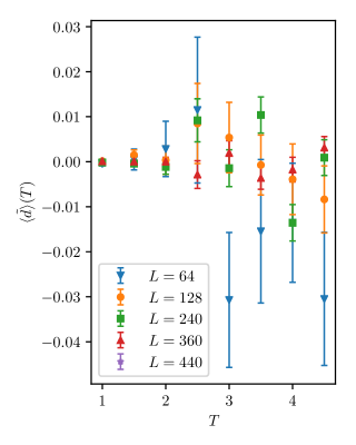
(a)

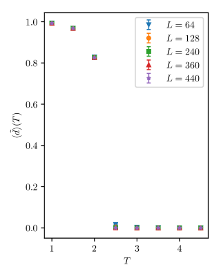
(b)

Figure 3: (Colour online) Behaviour of $\langle\tilde{d}\rangle(T)$ with a kernel of degree $n=1$ (left) and $n=2$ (right).

4.2 Separation ability

In this subsection, using different degree polynomial kernels, we evaluate the ability of the SVM to separate data through estimates of the expected risk, as explained in Sect. 3. Specifically, we will evaluate the empirical risk for homogeneous polynomial kernels of degrees $n=1,\dots,4$, for every value of the size $L$ and for every possible pair of training temperatures $T_{1}$ and $T_{2}>T_{1}$ in the coarse temperature scan discussed above.

In each case, we report estimates of the expected risk, also called the score, and of the ratio $\langle n_{\text{SV}}\rangle/n_{\text{TP}}$ between number of support vectors and the total number of points in the training sample. We estimate the latter with its statistical error using a jack-knife procedure that consists in computing the running averages after 10% of the points in each training set is removed; hence, in our case, $n_{\text{TP}}=360$, each complete training set consisting of $200$ points. The results are represented as heatmaps in Figs. 4, 5 and 6 for three different lattice sizes. In these figures, the lower training temperature $T_{1}$ is reported on the horizontal axis, the higher, $T_{2}$, on the vertical axis. For each pair, the obtained score is reported as the color of the corresponding rectangle in grayscale. A white rectangle maps to the poorest score of $0$, while a black rectangle to the maximum score of $1$. Note that a score of 0.5 is equivalent to a mere guess, and hence provides the worst possible classification ability. In addition, the average of the ratio $\langle n_{\text{SV}}\rangle/n_{\text{TP}}$ is shown as a number in the rectangle together with the measured error (unless the latter is exactly zero).

Let us discuss how to read these heatmaps. In each case, the values reported on the skew diagonal correspond to close training temperatures, while, at the opposite end, the values in the upper left corner correspond to distant pairs of training temperatures. Columns (resp. rows) correspond to scores obtained for various values of $T_{2}$ (resp. $T_{1}$) holding $T_{1}$ (resp. $T_{2}$) fixed.

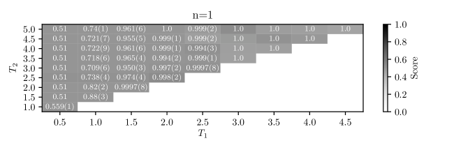
(a)

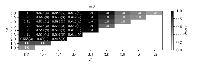
(b)

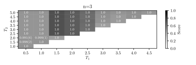
(c)

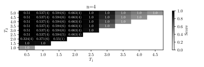
(d)

Figure 4: (Colour online) Heatmaps representing the score of the cross-validation test at $L=128$ and $C=1.0$ with homogeneous polynomial kernels of power $n=1,\dots,4$. The numbers in the rectangles are the estimates of $\langle n_{\text{SV}}\rangle/n_{\text{TP}}$.

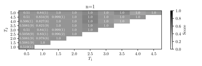
(a)

(b)

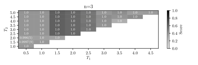
(c)

(d)

Figure 5: (Colour online) Heatmaps representing the score of the cross-validation test at $L=240$ and $C=1.0$ with homogeneous polynomial kernels of power $n=1,\dots,4$. The numbers in the rectangles are the estimates of $\langle n_{\text{SV}}\rangle/n_{\text{TP}}$.

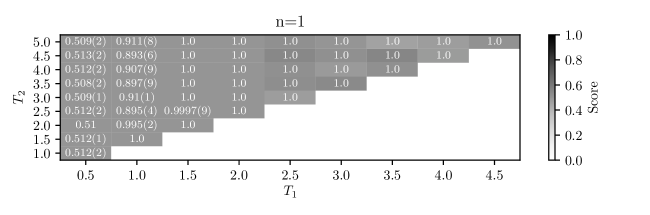
(a)

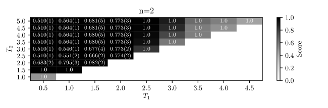
(b)

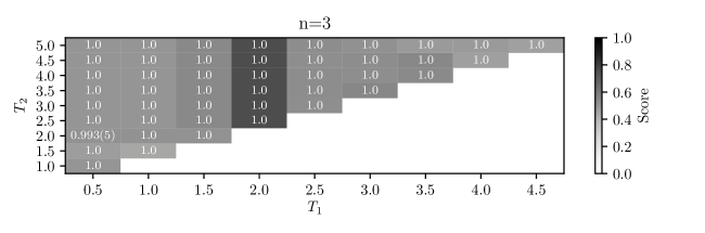
(c)

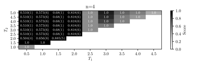
(d)

Figure 6: (Colour online) Heatmaps representing the score of the cross-validation test at $L=360$ and $C=1.0$ with homogeneous polynomial kernels of power $n=1,\dots,4$. The numbers in the rectangles are the estimates of $\langle n_{\text{SV}}\rangle/n_{\text{TP}}$.

Already at a first glance we notice that the SVM with a kernel of even degree ($n=2,4$) yields a better score than with kernels of odd degree ($n=1,3$) everywhere on the heatmaps. Let us analyse the even and the odd power kernel cases in more detail.

For the even degree kernels, the results seem to change only slightly among the various $L$ at $n=2$ and $n=4$. Therefore, we analyse the case $n=2$, $L=128$ and later comment on the differences with respect to $n=4$ and for larger $L$’s. The score is close to $1$ for almost every choice of the pair $T_{1}$ and $T_{2}$, except when they are both smaller than $T=2$ or both greater than $T=2.5$ and very close to each other. Note that in the critical region, the score remains high even when $T_{1}$ and $T_{2}$ are close. Regarding the ratio $\langle n_{\text{SV}}\rangle/n_{\text{TP}}$, we can divide the heatmap in roughly two regions. For $0.5\leq T_{1}\leq 2.0$ and $2.0<T_{2}\leq 5.0$, the ratio has a consistently lower value than in the rest of the heatmap, the difference being up to $\sim 30\%$. This is an additional hint at the fact that a transition may take place for $T\sim 2.0$. We remind the reader that our analysis in the previous section has singled out the value $T=2.5$, which is the next high up in our coarse scanning; hence, we can redefine the critical region as $2.0\leq T\leq 2.5$. Once again, for the moment this is just a convenience name, as we have not shown any evidence of any phase transition yet. In the critical region of the heatmap, the ratio $\langle n_{\text{SV}}\rangle/n_{\text{TP}}$ reaches its minimum value when $T_{1}$ and $T_{2}$ are the farthest possible, in the upper left hand corner, and its maximum value when the training temperatures are at their closest, in the bottom right hand corner.

In going to $n=4$ the picture is qualitatively the same, as it is for larger values of $L$. The only difference worth a comment is the behaviour of the number of support vectors for $T_{1}=0.5$ and $T_{2}=2.0$ at $n=4$, which is systematically lower than the value at $n=2$. As we can observe, however, the difference reduces at growing $L$ and we interpret it as an effect of the finite size of the system. Hence, we can infer that the estimate of the ratio $\langle n_{\text{SV}}\rangle/n_{\text{TP}}$ remains roughly constant even when the number of components of the feature map is increased considerably in passing from a quadratic to a quartic kernel. This means that of the new components of the feature map, almost none is chosen as support vector. This can be interpreted as the signal of the fact that the $n=2$ kernel already captures the essential properties of the model. It is then no surprise that increasing the number of components of the feature map does not lead to an improvement of the (already high) score. In that case, the new components of the feature map are actually fitting the statistical noise.

For the odd power kernels $n=1$ and $n=3$, the picture is totally different, the score being small over all the pairs $T_{1}$ and $T_{2}$. Let us analyse the case $n=1$ for $L=128$ first. The score is $\sim 0.5$ over all the heatmap. This means that the classification algorithm classifies incorrectly roughly half of the test samples. In passing to $n=3$, the score heatmap remains approximately the same, but the behaviour of the ratio $\langle n_{\text{SV}}\rangle/n_{\text{TP}}$ changes, and becomes almost uniformly $\sim 1.0$. This means that as a consequence of the addition of components to the feature map, almost the whole points in the sample become support vectors. Such a behaviour in passing from $n=1$ to $n=3$ is observed at all values of $L$. We argue that in those cases the minimisation algorithm uses the more numerous components of the $n=3$ feature map to try to fit to statistical noise, i.e. to overfit in order to accommodate a separating hypersurface. Hence, in this case we obtain a poorer classification prediction.

We have performed a similar analysis (not reported here) also with the $n=5$ and $n=6$ kernels, which confirms the conclusion that even power kernels are preferred to odd power kernels in terms of their efficiency at separating classes corresponding to temperatures. One can also easily see that, among the even degree kernels, the quadratic kernel performs better, in the sense of containing already all information on the separating hypersurface with the minimal number of features. This set of observations is very powerful at identifying the important symmetry at play. In fact, the common symmetry of the better performing kernels is $\mathbb{Z}_{2}$, and among all the $\mathbb{Z}_{2}$ symmetric kernels, the $n=2$ kernel is the one for which this symmetry is maximal, while all the others have higher order symmetries containing $\mathbb{Z}_{2}$ as a subgroup (namely, $\mathbb{Z}_{4}$ for $n=4$ and $\mathbb{Z}_{6}$ for $n=6$). Among the even power kernels, the behaviour of the number of support vectors singles out the quadratic kernel as the one that best adapts to the data.

It is worth stressing again at this point that $\mathbb{Z}_{2}$ invariance was not an input: indeed the SVM has been only fed with raw configurations, i.e. vectors with $L^{2}$ components labeled with the temperature, whose possible values are $\pm 1$. By clearly singling out the quadratic kernel, the SVM is giving us a strong hint of a possible global symmetry of the system. Hence, our working hypothesis that a systematic investigation of a class of kernels can identify the symmetry of the system seems to be valid.

4.3 Meaning of the decision function

Given the special role played by the $n=2$ kernel, we restrict our analysis to the latter from now on. As noted in [13], in the case of $n=2$, the meaning of the decision function can be easily understood. Its homogeneous part $\tilde{d}$ can be written as

$$\tilde{d}(\vec{x})=\frac{1}{2}\sum_{i=1}^{n_{SV}}y_{i}\alpha_{i}~{}\mathcal{K}\left(\vec{x}_{i},\vec{x}\right)=\frac{1}{2L^{4}}\sum_{i=1}^{n_{SV}}y_{i}\alpha_{i}~{}\left(\sum_{\vec{a}}x_{i}(\vec{a})\,x(\vec{a})\right)^{2}~{},$$ (53)

where on the right hand side we switched back to a cartesian labeling of the elementary variables, $\vec{a}$ indicating the position on the lattice and the sum running over the whole lattice. After swapping the sums over the positions with the sum over the support vectors, Eq. (51) can be rewritten as

$$\tilde{d}(\vec{x})=\frac{1}{2}\sum_{\vec{a},\vec{b}}C(\vec{a},\,\vec{b})\,x(\vec{a})\,x(\vec{b})~{},$$ (54)

where

$$\overline{C}(\vec{a},\,\vec{b})=\frac{1}{L^{4}}\sum_{i=1}^{n_{\text{SV}}}y_{i}\alpha_{i}\,x_{i}(\vec{a})\,x_{i}(\vec{b})\ .$$ (55)

The quantity $\overline{C}(\vec{a},\vec{b})$ can be interpreted as an effective coupling between two spins at positions $\vec{a}$ and $\vec{b}$ (see also [13]). As it can be verified by direct inspection, $\overline{C}(\vec{a},\vec{b})=\overline{C}(\vec{a}-\vec{b})$, owing to the translation symmetry of the system. By studying the average $\overline{C}(\vec{a})$ obtained by training a quadratic SVM at a given pair of training temperatures, we can get a clear insight into the nature of the decision function. An illustration of the behaviour of this quantity is provided in a normalised (from $0$ (lightest colour) to $1$ (darkest)) heatmap in Fig. 7 at $L=64$ for $C=1.0$ at four choices of the training temperatures. These can be seen as pictures of the effective coupling. Note that periodic boundary conditions are imposed in both directions.

Let us comment on these heatmaps. In all cases except one, the effective coupling is roughly uniform. Then

$$\tilde{d}(\vec{x})\propto\frac{1}{L^{4}}\sum_{\vec{a}}x(\vec{a})\,x(\vec{a})=m^{2}~{},$$ (56)

where $m$ is the magnetisation density of the system. The decision function $d$, in this case, is thus linearly related to $m^{2}$.

If $T_{1}$ and $T_{2}$ are respectively smaller and greater than $T=2.5$ (bottom right panel) but very close to each other, we see that the effective coupling vanishes smoothly in a small neighbourhood of the origin and is uniformly $1$ everywhere else. When, instead, $T_{1},T_{2}>2.5$, the shape of the effective coupling drastically changes. The decision function becomes now a shorter ranged version of $m^{2}$. These conclusions do not change for larger volumes and as long as $C\gtrsim 10^{-2}$. It is clear that the distinction between the decision functions learned in each case is related to its range on the lattice. The mapping of the decision function into the order parameter provides us with an easy a posteriori interpretation on the conclusion (reached in the previous two subsections) that learning temperatures must be chosen distant enough and on either side of $T=2.5$: with this choice, the SVM has information from both phases of the model, which enables it to learn the order parameter.

(a) $T_{1}=0.5$, $T_{2}=5.0$.

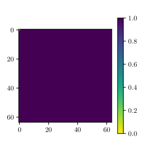
(b) $T_{1}=0.5$, $T_{2}=2.0$.

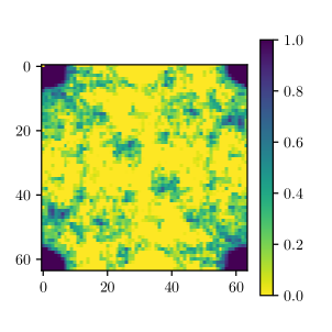
(c) $T_{1}=3.0$, $T_{2}=5.0$.

(d) $T_{1}=2.0$, $T_{2}=2.5$.

Figure 7: (Colour online) Heatmaps representing the effective coupling $\overline{C}({\vec{x}})$ for $L=64$ at the indicated values of the pairs $T_{1}$, $T_{2}$. The axes are the Cartesian coordinates of the lattice.

4.4 Extracting $T_{c}$ and the critical exponents

In this subsection, we shall show that the decision function can be used to precisely locate the phase transition point and evaluate the critical exponents. The heuristic argument that guides our approach is the following. Far from the phase transition, the SVM should easily succeed at classifying phases, as configurations will fall far from the separating hypersurface. Near the phase transition, we would expect a less clear classification, with configurations falling in the separating margin. The critical temperature can be identified with the temperature at which $\langle\tilde{d}\rangle$ has the maximal change (see e.g. Fig. 3). Hence, by studying the fluctuations of the decision function obtained following an appropriate training procedure (which is provided by a measure of the classification error), one can identify the critical temperature as the value at which this quantity reaches its maximum. Owing to finite size scaling, the shift of this maximal value as a function of $L$ is expected to scale with the critical exponent $\nu$ of the transition.

For the Ising model, the identification of $m^{2}$ as the decision function learned for distant temperatures on either side of $T=2.5$ provides a more rigorous justification of our heuristic expectations. Indeed, we know that the fluctuations of $m^{2}$ reach their peak at the critical temperature. Since $\tilde{d}$ is proportional to $m^{2}$, its fluctuations should show the same behaviour. Therefore, by performing a finer scan of temperatures in the critical region as identified in the procedure for calibrating the choice of the kernel, we should be able to find a peak in $\sigma_{d}$, the susceptibility of $d$, hence uncovering the phase transition. This will allow us to obtain $T_{c}(L)$ and the critical exponents.

Before showing our results, we remark that our discussion of the methodology allows us to identify also important potential sources of systematic errors. For instance, when instead of $m^{2}$ the learned decision function is a shorter range version thereof, as it happens e.g. when both training temperatures are in the symmetric phase, the fluctuations of $\tilde{d}$ will not be related to criticality, and the outcome of our analysis will be completely dominated by the systematics. We have shown that our procedure for choosing the training temperatures reasonably protects us from this extreme scenario. Other distortions to the learned decision function from the target one will arise if $T_{1}$ and $T_{2}$ are chosen too close to the critical region, as shown in the bottom right panel of Fig. 7. Although cross-validation and analysis of number of support vectors as the training temperatures vary provide reassuring evidence that we can avoid also this case, our determination of $T_{c}$ and of the critical exponents must take it into account as a logical possibility. Hence, while for brevity we shall show only results for one set of training temperatures (namely $T_{1}=0.5$ and $T_{2}=5.0$), in our study we ensured we are free from systematic errors related to the choice of the training points by testing our numerical values for robustness against changes of $T_{1}$ and $T_{2}$ in the pre-determined acceptable region.

We now move on to the determination of the critical temperature $T_{c}$ and of the critical exponents. In order to perform an easier comparison with the results obtained with standard methods for the magnetic susceptibility $\chi$, we consider the quantity

$$V\sigma_{d}=V\sqrt{\langle d^{2}\rangle-\langle d\rangle^{2}}\ .$$ (57)

From Eq. (53), we find

$$V\sigma_{d}\propto V\sqrt{\langle m^{4}\rangle-\langle m^{2}\rangle^{2}}=V\langle m^{2}\rangle\sqrt{\frac{\langle m^{4}\rangle}{\langle m^{2}\rangle^{2}}-1}\ .$$ (58)

Note that $\sigma_{d}$ and $\sigma_{\tilde{d}}$ are linearly related, owing to the definition of $\tilde{d}$.

Let us examine the scaling behaviour of $V\sigma_{d}$. The choice of $\Gamma$ in Eq. (50) ensures that the proportionality constant between $\tilde{d}$ and $m^{2}$ is independent of the volume. Hence, a straightforward dimensional analysis of Eq. (58) shows that the scaling behaviour of $V\sigma_{d}$ near criticality is the same as that of the magnetic susceptibility $\chi$,

$$V\sigma_{d}(T_{c}(L))\propto L^{\frac{\gamma}{\nu}}~{}\ ,$$ (59)

with

$$T_{c}-T_{c}(L)\propto L^{1/\nu}\ .$$ (60)

To obtain both the pseudocritical temperature $T_{c}(L)$ and the critical exponents $\gamma$ and $\nu$, it will then be sufficient to find the coordinates of the maximum of $V\sigma_{d}(L)$ in the $(T,V\sigma_{d})$ plane (which we refer to respectively as $T_{c}(L)$ and $V\sigma_{\text{d,max}}(T_{c})$) for each $L$ and fit Eq. (59) and Eq. (60) to their behaviour. For each value of $L$, $V\sigma_{\text{d,max}}(T_{c})$ and $T_{c}(L)$ are first roughly estimated and then their estimate is improved with a finer scan. To better compare the final results with those obtained with the multi-histogram method, we used the same temperatures used for this latter analysis, see Tab. 1.

The results of this procedure are reported in Tab. 3 and represented in Figs 8a and 8b. The scaling behaviour is fitted to the data using $T_{c}(L)$, $\nu$ and $\gamma/\nu$ as fitting parameters. The results of the fit are reported in Tab. 4 and plotted also in Figs. 8a and 8b. As an additional estimate of the critical temperature, also the fits with the critical exponents fixed to their analytical values are performed. The results are visible in the same figures and tables. The determined values of $T_{c}$, $\nu$ and $\gamma$ have good accuracy, which allows us to make meaningful comparisons with both the values obtained analytically for the 2D Ising model ($\gamma=7/4=1.75$ and $\nu=1$) and with the estimates obtained with the multi-histogram method. As in the conventional analysis, all the determined quantities are compatible with the analytical known values within at most two standard deviations. The errors on the fitted parameters obtained with the traditional approach are smaller by about a factor two to four than in the SVM analysis, possibly owing to the fact that the former method combines samples at different values of $T$ through multi-histogram reweighting, which can not be used in our Machine Learning analysis (since, for instance, in order to use it, we would need to know the Hamiltonian of the system, which is not part of our hypotheses). Likewise, the availability of more data for the fitting procedure generated through reweighting explains the smaller $\chi^{2}_{r}$ in the case of the conventional analysis, since in this latter case one has better resolution around the maximum.

Hence, to conclude, when applied to the same set of input data, our analysis shows that a finite size scaling study of the peak of the decision function susceptibility provides results that are quantitatively comparable for precision and accuracy to those obtained with a traditional finite size scaling analysis of the order parameter susceptibility using reweighting techniques. We note that our analysis for the extraction of $T_{c}$ and $\nu$ has only made use of an implicit connection between the decision function and the order parameter, while for the extraction of $\gamma/\nu$ the exact relationship has been needed.

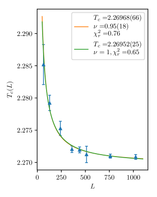
(a) (Colour online) Temperature of the peak value of $V\sigma_{d}$ at each simulated size $L$.

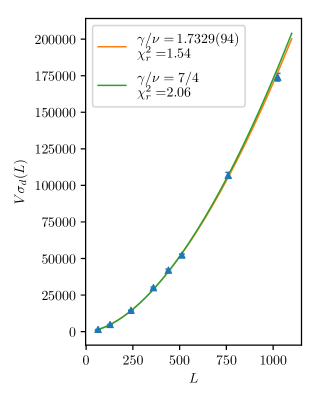
(b) (Colour online) Peak values of $V\sigma_{d}$ computed at each simulated size $L$.

Figure 8: Finite size scaling of critical quantities extracted from the SVM decision function error.

$L$	$T_{c}(L)$	$V\sigma_{d}$
$64$	$2.2852(31)$	$1.426(31)\cdot 10^{3}$
$128$	$2.2792(12)$	$4.782(85)\cdot 10^{3}$
$240$	$2.2753(11)$	$1.448(24)\cdot 10^{4}$
$360$	$2.27204(51)$	$2.995(55)\cdot 10^{4}$
$440$	$2.27194(46)$	$4.193(82)\cdot 10^{4}$
$512$	$2.2712(13)$	$5.221(87)\cdot 10^{4}$
$760$	$2.27098(31)$	$1.068(21)\cdot 10^{5}$
$1024$	$2.27085(38)$	$1.740(26)\cdot 10^{5}$

Table 3: Position ($T_{c}(L)$) and volume-multiplied value ($V\sigma_{d}$) of the maximum of the decision function error at each investigated lattice size $L$.

$T_{c}$	$\nu$	$\chi^{2}_{r}$	$\gamma/\nu$	$\chi^{2}_{r}$
$2.26968(66)$	$0.95(18)$	$0.79$	$1.733(10)$	$1.54$
$2.26954(25)$	$1$ (exact)	$0.65$	$7/4$ (exact)	$2.06$

Table 4: Results of the fit of the predicted scaling behaviour Eq. (59) and Eq. (60) to the data in Tab. 3. The best fit curves are represented in Figs. 8a and 8b.

5 Conclusions and outlook

In this work, we have provided the first (to the best of our knowledge) precision test of Machine Learning techniques applied to the study of phase transitions in statistical systems. In particular, we have studied the Ising model, benchmarking our findings with more consolidated numerical approaches that assume the knowledge of the Hamiltonian and of the order parameter. As a Machine Learning tool, we have used the Support Vector Machine, which implements a supervised learning technique. Our starting point are sets of configurations (with phase not specified, or unlabelled, using a Machine Learning language). The first task has been to understand whether a phase transition takes place. In order to perform this task, we needed to optimise the Machine Learning process by choosing a kernel to map input data in a space in which they are linearly separable. Looking at the performance of the separation process by choosing two arbitrary temperatures and giving them two different labels, we have been able to optimise the kernel and to deduce where a phase transition takes place. Our procedure of iterating over ordered pairs of training temperatures can be seen as a way to perform unsupervised learning using a supervised learning tool. Note that our approach is different from that of [13], where the phase was assumed to be known at various temperatures. In our case, the phase of the system is an output.

The optimised decision function, which is the learned classification criterium and is obtained through a systematic study of kernel performances using the optimal training temperatures, turns out to be simply related to the order parameter, with the kernel selection process and the optimal kernel pinning down the symmetry driving the phase transition. With the knowledge of the decision function, we have performed a finite size scaling analysis of its susceptibility (related to the classification error, expected to be maximal at the phase transition), obtaining results for the critical temperature and the critical exponents that are comparable in precision to those extracted with the best numerical tool currently available for studying phase transitions in systems with known Hamiltonian, namely finite size scaling of the order parameter susceptibility. Our extraction of the critical temperature and of the critical exponent $\nu$ describing the divergence of the correlation length has relied on the sole knowledge of the decision function and on the assumption that the latter is related to the order parameter, but not on the precise relationship between the two. This explicit relationship has been exploited to determine the combination $\gamma/\nu$.

Our results pave the way to precise quantitative studies of phase transitions using Machine Learning techniques, which are particularly useful in cases in which an order parameter is either not known or not existing, such as for topological phases of matters. There are several related directions in which this work can be extended. First, one can check whether the method of kernel selection we have proposed works in the Potts model, where the transition is driven by a $\mathbb{Z}_{N}$ symmetry, with $N\geq 3$. For $N=3$, we still expect a second order phase transition, but now the best performing kernel should be an homogeneous polynomial of order 3, with homogeneous polynomial of order 3n ($n>1$) still giving similar performance, while polynomials of order $3n+1$ and $3n+2$ ($n\geq 0$) should have significantly worse performance. In addition, for $N>4$, the system has a first order phase transition. Hence, in these cases it is not clear a priori if we can use the same methodology we have successfully devised for a second order phase transitions. Explorations in these directions are currently in progress. Another relevant question is how the proposed procedure can be generalised to systems with continuous symmetries, for which we would need to optimise the kernel in a wider space. Finally, it will be interesting to test our methodology on systems where a bona fide order parameter is absent or not known, like in models of topological superconductivity or in QCD with finite quark mass.

Appendix A Methodology

In this appendix, we discuss more technical aspects of the data analysis performed in Sects. 2 and 4.

A.1 Multi-histogram reweighting

In addition to providing an efficient way for computing thermodynamic observables, Monte Carlo simulations give direct information on the density of states $\rho(E)$ of a system, which can be extracted from an energy histogram of the generated configurations at a particular value of $\beta$. If $n(E)$ is the number of recorded events at energy $E$ and $N$ is the total number of generated events, the measured probability for the occurrence of energy $E$ is

$$p(E)=n(E)/N\ .$$ (61)

Since Monte Carlo are first principle methods, in the large $N$ limit this has to be equal to the Boltzmann probability. Hence,

$$\rho(E)=\frac{Z}{N}n(E)e^{\beta E}=\frac{n(E)}{N}e^{\beta E-f}\ ,$$ (62)

where $f=\beta F$ and $F$ is the free energy of the system.

In principle, determining $\rho(E)$ from a single simulation performed at a particular $\beta$ allows us to compute $Z$ (and then, to extract the thermodynamic properties of the system) at any other value of the temperature, since

$$Z(\beta^{\prime})=\sum_{E}\rho(E)e^{-\beta^{\prime}E}\ .$$ (63)

The approach of reconstructing thermodynamic observables at different $\beta$ from the density of states measured with histograms obtained in a single simulation is called single-histogram reweighting [50].

In practice, however, given that $E$ has Gaussian fluctuations around its average, in a simulation involving a finite set of configurations $\rho(E)$ can be extracted only in a limited range around the average energy, since the entries in the histogram will be unavoidably zero far enough from the central value of the Gaussian. On the other hand, this very same fact tells us that only a limited number of states with energy sufficiently close to the ensemble average Hamiltonian contribute in practice to the thermodynamics of a system at a given value of $\beta$. In order to cover the relevant range of energies needed at a particular temperature, one could do simulations at different values of $\beta=\beta_{1},\dots,\beta_{i},\dots,\beta_{j}$ for which the target density of states provides a non-negligible contribution to thermodynamic averaging of observables. For each of the simulated $\beta_{i}$ and fixed value of the energy $E_{k}$, we have

$$\rho_{i}(E_{k})=\frac{n_{i}(E_{k})}{N_{i}}e^{\beta_{i}E_{k}-f_{i}}\ ,$$ (64)

with $\rho_{i}(E_{k})$ being the density of states at energy $E_{k}$ measured in the run at $\beta_{i}$. Since all values of $\rho_{i}(E_{k})$ are an estimator for $\rho(E_{k})$, we can build the improved estimator

$$\rho(E_{k})=\sum_{i}r(i)\rho_{i}(E_{k})\ ,$$ (65)

with the weights $r(i)$ satisfying $\sum_{i}r(i)=1$. The $r(i)$ can be determined by minimising the square of the error in $\rho(E_{k})$, which gives

$$\rho(E_{k})=\frac{\sum_{i=1}^{j}g_{i}^{-1}n_{i}(E_{k})}{\sum_{i=1}^{j}N_{i}g_{i}^{-1}e^{\beta_{i}E_{k}-f_{i}}}\ ,$$ (66)

with the $f_{i}$ defined self-consistently using the relationship

$$e^{-\beta_{i}f_{i}}=\sum_{k}\rho(E_{k})e^{-\beta_{i}E_{k}}\ ,$$ (67)

$n_{i}(E_{k})$ the number of entries at energy $E_{k}$ recorded in the run performed at $\beta_{i}$ and $N_{i}$ the total number of configurations generated in the same run. In order to keep into account the autocorrelation time of each simulation, we have introduced the autocorrelation factor $g_{i}=1+2\tau_{i}$, where $\tau_{i}$ can be calculated e.g. with the Madras-Sokal algorithm [51]. The set of $2j$ simultaneous equations (66, 67) can be solved numerically (for instance, using the Newton-Raphson method). The expectation value of an observable $O$ at a reweighted $\beta$ can be expressed as

$$\langle O\rangle_{\beta}=\frac{\sum_{i=1}^{j}\sum_{l=1}^{N_{i}}g_{i}^{-1}O_{i}^{l}e^{-\beta E_{i}^{l}-f_{\beta}}}{\sum_{m=1}^{J}N_{m}g_{m}^{-1}e^{-\beta_{m}E_{i}^{l}+f_{m}}}\ ,$$ (68)

with

$$e^{-f_{\beta}\beta}=\frac{\sum_{i=1}^{j}\sum_{l=1}^{N_{i}}g_{i}^{-1}e^{-\beta E_{i}^{a}}}{\sum_{m=1}^{J}N_{m}g_{m}^{-1}e^{-\beta_{m}E_{i}^{a}+f_{m}}}\ ,$$ (69)

where all the $f_{j}$ (and $f_{\beta}$) are determined self-consistently. In the previous two equations $E_{i}^{l}$ indicates the value of the energy measured at Monte Carlo step $l$ in the run performed at $\beta_{i}$ and likewise $O_{i}^{l}$ is the value of $O$ at Monte Carlo step $l$ in the run at $\beta_{i}$. This method, introduced in [52], is known as multi-histogram reweighting.

While multi-histogram reweighting has a wider range of predictability and generally better precision than the single-histogram method, there are still technical points to consider in order to apply the former technique efficiently. In particular, each density of state value will receive contributions only from simulations at which the corresponding energy is sampled with sufficient accuracy. Notwithstanding this and other limitations, if carefully implemented, multi-histogram reweighting is a powerful tool for extracting to a very high degree of accuracy quantities related to phase transitions such as critical exponents and critical couplings from Monte Carlo simulations. While the obtained accuracy depends on the details of the calculations (like the number of sampled $\beta$’s in the critical region and the number of configurations generated at each $\beta$, in addition to the chosen Monte Carlo update algorithm), precisions well below the percent level on critical exponents and significantly higher on critical couplings are within reach for a wide number of statistical systems.

A.2 Bootstrap

The bootstrap technique is a general procedure that can be used to obtain robust estimates of the standard error from observations of variables even when the underlying probability distribution is unknown. This technique proves particularly convenient when we are interested in general functions of a random variable.

Let us assume we have a set of measurements of the variable X, described by the ensamble $\{X_{i}\}$, $1\leq i\leq N$, with $N$ the total number of measurements. We are interested in the estimator of $F(X)$, where $F$ is a function of the variable $X$. The bootstrap provides the estimator and the confidence interval according to the following procedure:

1. build the set of the estimators $\{F_{i}=F(X_{i})\}\$;

2. for each $j$ with $1\leq j\leq N_{B}$, with $N_{B}$ integer, construct a bootstrap sample by taking $N$ random values in $\{F_{i}\}$ and call the resulting set $\{F^{j}_{i}\}$ (each of this sets will be referred to as a bootstrap resample);

3. for each bootstrap resample $\{F^{j}_{i}\}$, compute the average as

   $$\overline{F}^{j}=\frac{1}{N}\sum_{i}F^{j}_{i}\ ;$$ (70)

4. an estimator for $F(X)$ is provided by the bootstrap average

   $$\bar{F}=\frac{1}{N_{B}}\sum_{j}\bar{F}^{j}\ ,$$ (71)

   with the standard error given by

   $$\Delta\bar{F}=\sqrt{\frac{1}{N_{B}-1}\sum_{j}\left(\bar{F}^{j}-\bar{F}\right)^{2}}\ .$$ (72)

In practical applications, one takes $N_{B}$ of the order of 100-1000, which ensures we fulfil the hypotheses of the central limit theorem.

Our discussion so far assumes lack of correlations between the data, which is certainly not the case for Monte Carlo generated data. In order to remove correlations from the sample, one applies a binning procedure, which consists in computing averages over $N_{b}$ consecutive values of $F_{i}$ and replace the latter subset of values with this average. This reduces the size of the sample of the $F_{i}$ used in the bootstrap procedure from $N$ to $N/N_{b}$. If we choose $N_{b}\gg\tau$, with $\tau$ the autocorrelation time, the data in the reduced set are uncorrelated. We can then apply the bootstrap procedure to the sample of the binned values.

References

References

- [1] S. Blundell, K. M. Blundell, Concepts in thermal physics, 2nd Edition, Oxford University Press, 2010.
- [2] H. Schawe, R. Bleim, A. Hartmann, Phase transitions of the typical algorithmic complexity of the random satisfiability problem studied with linear programming. arXiv:1702.02821.
- [3] R. Solé, Phase Transitions, Princeton University Press, 2011.
- [4] K. G. Wilson, J. B. Kogut, The Renormalization group and the epsilon expansion, Phys. Rept. 12 (1974) 75–200. doi:10.1016/0370-1573(74)90023-4.
- [5] J. Cardy, Scaling and Renormalization in Statistical Physics, Cambridge Lecture Notes in Physics, Cambridge University Press, 1996.
- [6] K. Langfeld, B. Lucini, R. Pellegrini, A. Rago, An efficient algorithm for numerical computations of continuous densities of states, Eur. Phys. J. C76 (6) (2016) 306. arXiv:1509.08391, doi:10.1140/epjc/s10052-016-4142-5.
-
[7]
M. A. Continentino,
Topological
phase transitions, Physica B: Condensed Matter 505 (2017) A1 – A2.
doi:https://doi.org/10.1016/j.physb.2016.10.037.
URL http://www.sciencedirect.com/science/article/pii/S0921452616305117 - [8] M. D’Elia, A. Di Giacomo, B. Lucini, G. Paffuti, C. Pica, Color confinement and dual superconductivity of the vacuum. IV., Phys. Rev. D71 (2005) 114502. arXiv:hep-lat/0503035, doi:10.1103/PhysRevD.71.114502.
-
[9]
J. Carrasquilla, R. G. Melko,
Machine learning phases of
matter, Nature Physics 13 (2017) 431 EP –.
URL http://dx.doi.org/10.1038/nphys4035 -
[10]
L. Wang, Discovering
phase transitions with unsupervised learning, Phys. Rev. B 94 (2016) 195105.
doi:10.1103/PhysRevB.94.195105.
URL https://link.aps.org/doi/10.1103/PhysRevB.94.195105 - [11] A. Tanaka, A. Tomiya, Detection of phase transition via convolutional neural network, J. Phys. Soc. Jap. 86 (6) (2017) 063001. arXiv:1609.09087, doi:10.7566/JPSJ.86.063001.
- [12] E. P. L. van Nieuwenburg, Y.-H. Liu, S. D. Huber, Learning phase transitions by confusion, Nature Physics 13 (2017) 435–439. arXiv:1610.02048, doi:10.1038/nphys4037.
-
[13]
P. Ponte, R. G. Melko,
Kernel methods for
interpretable machine learning of order parameters, Phys. Rev. B 96 (2017)
205146.
doi:10.1103/PhysRevB.96.205146.
URL https://link.aps.org/doi/10.1103/PhysRevB.96.205146 - [14] P. Broecker, F. F. Assaad, S. Trebst, Quantum phase recognition via unsupervised machine learningarXiv:1707.00663.
- [15] S. J. Wetzel, M. Scherzer, Machine Learning of Explicit Order Parameters: From the Ising Model to SU(2) Lattice Gauge Theory, Phys. Rev. B96 (18) (2017) 184410. arXiv:1705.05582, doi:10.1103/PhysRevB.96.184410.
-
[16]
S. J. Wetzel,
Unsupervised
learning of phase transitions: From principal component analysis to
variational autoencoders, Phys. Rev. E 96 (2017) 022140.
doi:10.1103/PhysRevE.96.022140.
URL https://link.aps.org/doi/10.1103/PhysRevE.96.022140 -
[17]
W. Hu, R. R. P. Singh, R. T. Scalettar,
Discovering
phases, phase transitions, and crossovers through unsupervised machine
learning: A critical examination, Phys. Rev. E 95 (2017) 062122.
doi:10.1103/PhysRevE.95.062122.
URL https://link.aps.org/doi/10.1103/PhysRevE.95.062122 - [18] A. Morningstar, R. G. Melko, Deep Learning the Ising Model Near Criticality, arXiv e-prints (2017) arXiv:1708.04622arXiv:1708.04622.
-
[19]
M. J. S. Beach, A. Golubeva, R. G. Melko,
Machine learning
vortices at the kosterlitz-thouless transition, Phys. Rev. B 97 (2018)
045207.
doi:10.1103/PhysRevB.97.045207.
URL https://link.aps.org/doi/10.1103/PhysRevB.97.045207 - [20] M. Richter-Laskowska, H. Khan, N. Trivedi, M. M. Maśka, A machine learning approach to the Berezinskii-Kosterlitz-Thouless transition in classical and quantum models, arXiv e-prints (2018) arXiv:1809.09927arXiv:1809.09927.
- [21] S. Iso, S. Shiba, S. Yokoo, Scale-invariant Feature Extraction of Neural Network and Renormalization Group Flow, Phys. Rev. E97 (5) (2018) 053304. arXiv:1801.07172, doi:10.1103/PhysRevE.97.053304.
- [22] K. Kashiwa, Y. Kikuchi, A. Tomiya, Phase transition encoded in neural networkarXiv:1812.01522.
- [23] G. Cossu, L. Del Debbio, T. Giani, A. Khamseh, M. Wilson, Machine learning determination of dynamical parameters: The Ising model casearXiv:1810.11503.
-
[24]
T. Ohtsuki, T. Ohtsuki, Deep
learning the quantum phase transitions in random two-dimensional electron
systems, Journal of the Physical Society of Japan 85 (12) (2016) 123706.
arXiv:https://doi.org/10.7566/JPSJ.85.123706, doi:10.7566/JPSJ.85.123706.
URL https://doi.org/10.7566/JPSJ.85.123706 -
[25]
T. Mano, T. Ohtsuki, Phase
diagrams of three-dimensional anderson and quantum percolation models using
deep three-dimensional convolutional neural network, Journal of the Physical
Society of Japan 86 (11) (2017) 113704.
arXiv:https://doi.org/10.7566/JPSJ.86.113704, doi:10.7566/JPSJ.86.113704.
URL https://doi.org/10.7566/JPSJ.86.113704 -
[26]
F. Schindler, N. Regnault, T. Neupert,
Probing many-body
localization with neural networks, Phys. Rev. B 95 (2017) 245134.
doi:10.1103/PhysRevB.95.245134.
URL https://link.aps.org/doi/10.1103/PhysRevB.95.245134 - [27] P. Broecker, J. Carrasquilla, R. G. Melko, S. Trebst, Machine learning quantum phases of matter beyond the fermion sign problem, Scientific Reports 7 (2017) 8823. arXiv:1608.07848, doi:10.1038/s41598-017-09098-0.
-
[28]
K. Ch’ng, J. Carrasquilla, R. G. Melko, E. Khatami,
Machine learning
phases of strongly correlated fermions, Phys. Rev. X 7 (2017) 031038.
doi:10.1103/PhysRevX.7.031038.
URL https://link.aps.org/doi/10.1103/PhysRevX.7.031038 -
[29]
Y. Zhang, E.-A. Kim,
Quantum loop
topography for machine learning, Phys. Rev. Lett. 118 (2017) 216401.
doi:10.1103/PhysRevLett.118.216401.
URL https://link.aps.org/doi/10.1103/PhysRevLett.118.216401 - [30] Y. Zhang, R. G. Melko, E.-A. Kim, Machine learning Z2 quantum spin liquids with quasiparticle statistics, Phys. Rev. B96 (24) (2017) 245119, [Addendum: Phys. Rev.B97,no.7,079904(2018)]. arXiv:1705.01947, doi:10.1103/PhysRevB.96.245119,10.1103/PhysRevB.97.079904.
-
[31]
N. Yoshioka, Y. Akagi, H. Katsura,
Learning
disordered topological phases by statistical recovery of symmetry, Phys.
Rev. B 97 (2018) 205110.
doi:10.1103/PhysRevB.97.205110.
URL https://link.aps.org/doi/10.1103/PhysRevB.97.205110 -
[32]
S. Arai, M. Ohzeki, K. Tanaka,
Deep neural network detects
quantum phase transition, Journal of the Physical Society of Japan 87 (3)
(2018) 033001.
arXiv:https://doi.org/10.7566/JPSJ.87.033001, doi:10.7566/JPSJ.87.033001.
URL https://doi.org/10.7566/JPSJ.87.033001 -
[33]
J. Greitemann, K. Liu, L. Pollet,
Probing hidden
spin order with interpretable machine learning, Phys. Rev. B 99 (2019)
060404.
doi:10.1103/PhysRevB.99.060404.
URL https://link.aps.org/doi/10.1103/PhysRevB.99.060404 -
[34]
K. Liu, J. Greitemann, L. Pollet,
Learning multiple
order parameters with interpretable machines, Phys. Rev. B 99 (2019) 104410.
doi:10.1103/PhysRevB.99.104410.
URL https://link.aps.org/doi/10.1103/PhysRevB.99.104410 -
[35]
J. Carrasquilla, Viewpoint: Neural
networks identify topological phases, Physics 10 (2017) 56.
URL http://dx.doi.org/10.1038/nphys4035 -
[36]
U. Wolff, Collective
monte carlo updating for spin systems, Phys. Rev. Lett. 62 (1989) 361–364.
doi:10.1103/PhysRevLett.62.361.
URL https://link.aps.org/doi/10.1103/PhysRevLett.62.361 - [37] D. Landau, K. Binder, A Guide to Monte Carlo Simulations in Statistical Physics, Cambridge University Press, 2014.
- [38] C. Cortes, V. Vapnik, Support-vector networks, Machine learning 20 (3) (1995) 273–297.
- [39] B. E. Boser, I. M. Guyon, V. N. Vapnik, A training algorithm for optimal margin classifiers, in: Proceedings of the fifth annual workshop on Computational learning theory, ACM, 1992, pp. 144–152.
-
[40]
V. Pappu, P. M. Pardalos,
High-Dimensional Data
Classification, Springer New York, New York, NY, 2014, pp. 119–150.
doi:10.1007/978-1-4939-0742-7\_8.
URL https://doi.org/10.1007/978-1-4939-0742-7_8 - [41] J. Shawe-Taylor, N. Cristianini, Kernel methods for pattern analysis, Cambridge university press, 2004.
- [42] V. Kecman, Learning and soft computing: support vector machines, neural networks, and fuzzy logic models, MIT press, 2001.
- [43] W. Karush, M.Sc. Dissertation, Dept. of Mathematics, University of Chicago, Chicago, Illinois (US), 1939.
-
[44]
H. W. Kuhn, A. W. Tucker,
Nonlinear
programming, in: Proceedings of the Second Berkeley Symposium on
Mathematical Statistics and Probability, University of California Press,
Berkeley, Calif., 1951, pp. 481–492.
URL https://projecteuclid.org/euclid.bsmsp/1200500249 -
[45]
B. Haasdonk, H. Burkhardt,
Invariant kernel functions
for pattern analysis and machine learning, Machine Learning 68 (1) (2007)
35–61.
doi:10.1007/s10994-007-5009-7.
URL https://doi.org/10.1007/s10994-007-5009-7 - [46] H. Schulz-Mirbach, On the existence of complete invariant feature spaces in pattern recognition, Tech. rep., Hamburg, Germany, Germany (1992).
- [47] B. Scholkopf, A. J. Smola, Learning with Kernels: Support Vector Machines, Regularization, Optimization, and Beyond, MIT Press, Cambridge, MA, USA, 2001.
-
[48]
R. Kohavi, A study of
cross-validation and bootstrap for accuracy estimation and model selection,
in: Proceedings of the 14th International Joint Conference on Artificial
Intelligence - Volume 2, IJCAI’95, Morgan Kaufmann Publishers Inc., San
Francisco, CA, USA, 1995, pp. 1137–1143.
URL http://dl.acm.org/citation.cfm?id=1643031.1643047 - [49] F. Pedregosa, G. Varoquaux, A. Gramfort, V. Michel, B. Thirion, O. Grisel, M. Blondel, P. Prettenhofer, R. Weiss, V. Dubourg, J. Vanderplas, A. Passos, D. Cournapeau, M. Brucher, M. Perrot, E. Duchesnay, Scikit-learn: Machine learning in Python, Journal of Machine Learning Research 12 (2011) 2825–2830.
-
[50]
A. M. Ferrenberg, R. H. Swendsen,
New monte carlo
technique for studying phase transitions, Phys. Rev. Lett. 61 (1988)
2635–2638.
doi:10.1103/PhysRevLett.61.2635.
URL https://link.aps.org/doi/10.1103/PhysRevLett.61.2635 -
[51]
N. Madras, A. D. Sokal, The pivot
algorithm: A highly efficient monte carlo method for the self-avoiding walk,
Journal of Statistical Physics 50 (1) (1988) 109–186.
doi:10.1007/BF01022990.
URL https://doi.org/10.1007/BF01022990 -
[52]
A. M. Ferrenberg, R. H. Swendsen,
Optimized monte
carlo data analysis, Phys. Rev. Lett. 63 (1989) 1195–1198.
doi:10.1103/PhysRevLett.63.1195.
URL https://link.aps.org/doi/10.1103/PhysRevLett.63.1195