ACACIA: a new method to produce on-the-fly merger trees in the RAMSES code

Abstract

The implementation of ACACIA, a new algorithm to generate dark matter halo merger trees with the Adaptive Mesh Refinement (AMR) code RAMSES, is presented. The algorithm is fully parallel and based on the Message Passing Interface (MPI). As opposed to most available merger tree tools, it works on the fly during the course of the N body simulation. It can track dark matter substructures individually using the index of the most bound particle in the clump. Once a halo (or a sub-halo) merges into another one, the algorithm still tracks it through the last identified most bound particle in the clump, allowing to check at later snapshots whether the merging event was definitive, or whether it was only temporary, with the clump only traversing another one. The same technique can be used to track orphan galaxies that are not assigned to a parent clump anymore because the clump dissolved due to numerical over-merging. We study in detail the impact of various parameters on the resulting halo catalogues and corresponding merger histories. We then compare the performance of our method using standard validation diagnostics, demonstrating that we reach a quality similar to the best available and commonly used merger tree tools. As a proof of concept, we use our merger tree algorithm together with a parametrised stellar-mass-to-halo-mass relation and generate a mock galaxy catalogue that shows good agreement with observational data.

1 Introduction

Mock galaxy catalogues generated using N-body or hydrodynamical simulations are important tools for extragalactic astronomy and cosmology. They are used to test current theories of galaxy formation, to explore systematic and statistical errors in large scale galaxy surveys and to prepare analysis codes for future dark energy mission such as Euclid or LSST. There is a large variety of methods to generate such mock galaxy catalogues. The most ambitious line of products is based on full hydrodynamical simulations, where dark matter, gas, and star formation are directly simulated (e.g. Dubois et al., 2014; Khandai et al., 2015; Vogelsberger et al., 2014; Schaye et al., 2015). The intermediate approach is based on semi-analytic modelling (hereafter SAM) (e.g. White & Frenk, 1991; Bower et al., 2006; Somerville & Primack, 1999; Kauffmann et al., 1993; Kang et al., 2005; Croton et al., 2006) for which galaxy formation physics, although simplified, is still at the origin of the mock galaxy properties. Finally, the simplest and most flexible approach is based on a purely empirical modelling of galaxy properties, sometimes called Halo Occupation Density (HOD hereafter) (e.g. Seljak, 2000; Berlind & Weinberg, 2002; Peacock & Smith, 2000; Benson et al., 2000; Wechsler et al., 2001; Scoccimarro et al., 2001). The last two techniques (SAM and HOD) both require the complete formation history of dark matter haloes, and possibly their sub-haloes. This formation history is described by halo ‘merger trees’ (Roukema et al., 1993; Roukema & Yoshii, 1993; Lacey & Cole, 1993). Accurate merger trees are essential to obtain realistic mock galaxy catalogues, and constitute the backbone of SAM and HOD models.

The advantage of using SAM and HOD techniques to generate mock galaxy catalogues is that one does not need to model explicitly the gas component, but only the dark matter component. The corresponding N-body simulations are commonly referred to as ‘dark matter only’ (DMO) simulations. With growing processing power, improved algorithms and the use of parallel computing tools and architectures, larger and better resolved DMO simulations are becoming possible. The current state-of-the-art is the Flagship simulation performed for the preparation of the Euclid mission (Potter et al., 2017) and featured 2 trillion dark matter particles. Such extreme simulations make post-processing analysis tool such as merger tree algorithms increasingly difficult to develop and to use, mostly because of the sheer size of the data to store on disk and to load up later from the same disk back into the processing unit memory. In some extreme cases, the amount of data that needs to be stored to perform a merger tree analysis in post-processing is simply too large. Storing just particle positions and velocities in single precision for trillions of particles requires dozens of terabytes per snapshot. Another issue is that most modern astrophysical simulations are executed on large supercomputers which offer large distributed memory. Post-processing the data they produce may also require just as much memory, so that the analysis will also have to be executed on the distributed memory infrastructures as well. The reading and writing of such vast amount of data to a permanent storage remains a considerable bottleneck, particularly so if the data needs to be read and written multiple times. One way to reduce the computational cost is to include analysis tools like halo-finding and the generation of merger trees in the simulations and run them “on the fly”, i.e. run them during the simulation, while the necessary data is already in memory.

The main motivation for this work is precisely the necessity for such a merger tree tool for future “beyond trillion particle” simulations. While many state-of-the-art N-body simulation codes include structure finders that are run on-the-fly, codes like Gadget4 Springel et al. (2021) who are able to build merger trees on-the-fly are still a relative rarity. It is crucial that multiple, distinct, codes have the capacity to do this to provide the possibility to cross-check results and their convergence. To this end, a new algorithm that we named ACACIA was designed to work on the fly within the parallel AMR code RAMSES. One novel aspect of this work is the use of the halo finder PHEW (Bleuler et al., 2015) for the parent halo catalogue. Different halo finders have been shown to have a strong impact on the quality of the resulting merger trees (Avila et al., 2014). PHEW falls into the category of “watershed” algorithms that are not so common in the cosmological halo finding literature. This type of algorithm assigns particles (or grid cells) to density peaks above a prescribed density threshold and according to the so-called “watershed segmentation” of the negative density field.

This paper is structured as follows. In Section 2, a brief description of the PHEW halo finder and its new particle unbinding method is given. Section 3 describes some common difficulties that arise when making merger trees and the way we address them in our merger algorithm ACACIA, which is ultimately described in detail in Section 4. Section 5 shows test results to determine what parameters give the best results. Using the halo catalogue and its corresponding merger tree generated on the fly by a cosmological N-body simulation, we use the stellar-mass-to-halo-mass (SMHM) relation from Behroozi et al. (2013c) to produce a mock galaxy catalogue. We analyse in Section 6 the properties of our mock galaxy catalogue and show that the introduction of orphan galaxies improve the comparison to observations considerably. Finally, a detailed comparison with the other halo finding and tree-building algorithms presented in Avila et al. (2014) is given in Appendix A.

2 Halo Finding and Particle Unbinding

Halo finding plays a central role in the exploitation of N-body simulations. Paradoxically, a unique definition of what is a halo or a sub-halo has never been adopted so far. The current state of affairs in the halo finding business is quite the opposite, with a multitude of definitions emerging over the last decades, each definition corresponding to a different halo finding algorithm. The Halo Finder Comparison Project (Knebe et al., 2011) lists 29 different codes and roughly divides them into two distinct groups:

1. Percolation algorithms, for which particles are linked together if closer to each other than some specified linking length. The typical example is the algorithm “friends-of-friends” (thereafter FOF) (Davis et al., 1985).

2. Segmentation algorithms, for which space is segmented into separate regions around local peaks of the density field. Particles within these regions are then collected and assigned to the same halo or sub-halo. The typical example is the “Spherical Overdensity” method (thereafter SOD) (Press & Schechter, 1974).

The outer boundary of the haloes are defined in both method by a density iso-surface, whose exact value determines the properties of the resulting halo statistics. Halo catalogues derived from FOF and SOD and their corresponding merger trees have been studied quite extensively in the literature (see e.g. Avila et al., 2014).

2.1 The PHEW halo finder

In this paper, we extend these earlier studies to the PHEW halo finder (Bleuler et al., 2015) developed specifically for the RAMSES code (Teyssier, R., 2002). The PHEW algorithm belongs to the category of segmentation methods. Particle masses are first deposited to the AMR grid using the “cloud-in-cell” technique. All density maxima are then marked as potential sites for a clump. Clumps are what we call any structure, haloes and sub-haloes, in contexts where we don’t need to differentiate between them. The volume is then segmented into peak patches by assigning each cell of the grid to the closest density maximum in the direction of the steepest density gradient.

This segmentation method provides well defined regions separated by density saddle surfaces. The minimum density in the saddle surface between two adjacent peaks marks the saddle point between the two peaks. This well known method is often called ‘watershed segmentation‘. In order to define proper halo boundaries, PHEW uses an outer density isosurface, like most methods described above. Subhaloes, on the other hand, are just the ensemble of all peak patches within the halo boundaries. This allows to identify haloes and sub-haloes without the assumption of spherical symmetry, unlike other popular methods such as SOD.

Subhaloes can be organised into a hierarchy of sub-structures based on the same steepest gradient technique, for which individual clumps can be assigned to the closest densest peak. After this first pass, only a few sub-haloes survived the merging process, which is then repeated a second time, assigning these surviving sub-haloes to their densest neighbours. Ultimately, all sub-haloes will be collected into a single peak that corresponds to the main halo. Each pass defines a level in the hierarchy of sub-haloes. More details can be found in the original PHEW paper (Bleuler et al., 2015). As a consequence, a halo can have a number of sub-haloes, each one of them containing subsub-haloes and so on. This well defined hierarchy is a very important feature for us to uniquely assign particles to haloes and sub-haloes based on a binding energy criterion.

There are four parameters that PHEW requires a user to choose in order to identify clumps and haloes. Firstly, a “relevance threshold” needs to be defined. If for any given peak patch the ratio of the peak’s density to the maximal density of the entire saddle surface of the respective peak patch is smaller than the chosen relevance threshold, then the peak patch is considered to be noise, not a genuine structure. The peak patch is then merged into a neighbour. Secondly, a density threshold determines the minimal density a cell needs to have to be part of any peak patch. Thirdly, a “saddle threshold” defines the maximal density for a saddle surface between two peak patches for the two patches to be considered parts of two different haloes. If the saddle surface density is above the threshold, then the peak patches will be parts of the same halo (but different sub-haloes within the host halo). Finally, a mass threshold determines the minimal mass a peak patch needs to have to be kept. We list the parameters that we used throughout this paper in Table 1.

Table 1: Parameters used for the PHEW clump finder throughout this paper. The numerical values given can be directly used in the namelist file that RAMSES uses to read in runtime parameters. Here $\bar{\rho}$ here is the mean background density and $m_{p}$ is the particle mass.

parameter	value	units
relevance threshold	3	1
density threshold	80	$\bar{\rho}$
saddle threshold	200	$\bar{\rho}$
mass threshold	10	$m_{p}$

2.2 Particle unbinding

We now describe how we assign each dark matter particle to a given sub-halo, a process that has not been implemented so far in the PHEW code. For this, we follow a physically motivated criterion, quite common in the halo finding literature, based on the binding energy of the particle (e.g. Knollmann & Knebe, 2009; Springel et al., 2001; Stadel, 2001). If a particle is not bound to the first sub-halo of the hierarchy, it is then passed recursively to the next sub-halo in the hierarchy, where the binding energy is checked again and so on. If the particle is not bound to any sub-halo, it is assigned to the main halo.

In the previous hierarchical unbinding process, the key component is the criterion adopted for deciding whether a particle is bound to a sub-halo or not. Traditionally, this is done using the static gravitational potential, since we are dealing with a single time step and we have to assume that the N-body system is stationary. In this case, a particle at position ${\bf r}$ is considered as unbound if its velocity ${\bf v}$ exceeds the escape velocity given by

$$v_{\rm esc}=\sqrt{-2\Phi(\mathbf{r})}$$ (1)

More precisely, this means that the particle will be able to travel to infinity where the potential goes to zero. If the velocity is smaller than the escape velocity, the particle will follow a bound orbit and come back to its current location. Note that this orbit can leave the boundaries of the sub-halo. The particle will stay for some time in the sub-halo, but can visit at a later time a neighbouring sub-halo and then come back along the same bound orbit. This kind of particle does not exclusively belong to its original sub-halo. It should be in fact assigned to the parent sub-halo in the hierarchy. In order to identify particles as more strictly bound, we re-define the escape velocity using the potential of the closest saddle point $\Phi_{S}$.

$$v_{\rm esc}=\sqrt{-2(\Phi(\mathbf{r})-\Phi_{S})}$$ (2)

This new escape velocity is smaller than the previous one, allowing more particle to exceed it and leak out of the current sub-halo into neighbouring ones. In what follows, we will use these two unbinding criteria, calling the first method the “loosely bound” criterion and calling the second one the “strictly bound” criterion. Figure 1 illustrates the difference between these two criteria. The gravitational potential of two neighbouring sub-haloes labelled A and B is represented. We show an example of a strictly bound particle in each sub-halo, and an example of a loosely bound particle that can wander from one sub-halo to the other one. If one uses the first binding criterion, this loosely bound particle will be assigned to sub-halo A, because this is where it is located at the present time. If one uses the second, stricter binding criterion, then the loosely bound particle will be assigned to the parent halo, but not to sub-halo A nor B.

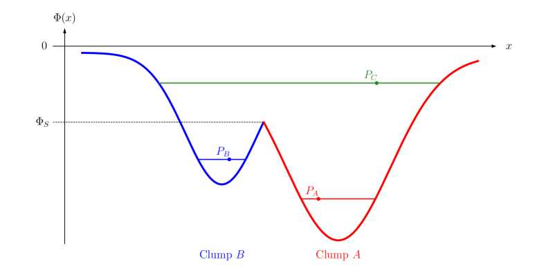
Figure 1: Simple sketch of the gravitational potential of a halo that consists of two clumps, $A$ and $B$. The position of the horizontal lines marks the energies of three example particles, $P_{A}$, $P_{B}$, and $P_{C}$, while the length of the lines shows the spatial extent of the orbits. We call particles like $P_{A}$ and $P_{B}$ “strictly bound”, as their predicted orbit boundaries don’t allow them to escape from the clump they are assigned to. Particle $P_{C}$ however, although energetically bound to clump $A$, can wander off deep into clump $B$, and for that reason is called “loosely bound”. To discriminate between these two types of particles, we use the potential of the saddle point between clump $A$ and $B$ marked as $\Phi_{S}$.

When computing the velocity of the particle, it is important to use the velocity relative to the velocity of the sub-halo centre of mass (also called the bulk velocity of the sub-halo). Because of this requirement, the unbinding process has to be performed iteratively, since removing a particle that is unbound requires to recompute the centre of mass velocity. Let us finally repeat that the particle unbinding is performed recursively, following the sub-halo hierarchy from the bottom up. Starting with the lowest (finest) level of sub-haloes, unbound particles are assigned to the higher (coarser) level of parent sub-halo for unbinding, and so on following the structure hierarchy. Particles that are unbound from all sub-haloes are collected into the main halo, marking the end of the hierarchical unbinding process.

3 Merger Trees: Basic Principles

In this work, we adopt the terminology set by the “Sussing Merger Tree Comparison Project” (Srisawat et al., 2013; Wang et al., 2016; Avila et al., 2014; Lee et al., 2014). For sake of clarity, we repeat here some important definitions:

• For two snapshots at different times, a halo from the first one (i.e. higher redshift) is always referred to using the capital letter $A$ and a halo from the second one (i.e. lower redshift) using $B$.

• Recursively, $A$ itself and progenitors of $A$ are all progenitors of $B$. When it is necessary to distinguish $A$ from earlier progenitors, the term direct progenitor will be used.

• Recursively, $B$ itself and descendants of $B$ are all descendants of $A$. When it is necessary to distinguish $B$ from later descendants, the term direct descendant will be used.

• In this work, we restrict ourselves to merger trees for which there is precisely one direct descendant for every halo.

• When there are multiple direct progenitors, it is required that one of these is identified as the main progenitor.

• The main branch of a halo is a complete list of main progenitors tracing back along its cosmic history.

We finally define an important convention we use here: when no distinction between sub-haloes and main haloes is necessary, they are collectively referred to as clumps.

3.1 Linking Clumps Across Snapshots

The aim of a merger tree code is to link haloes from an earlier snapshot to haloes in the consecutive snapshot, i.e. to find all the descendants of the haloes in the earlier snapshot. If we do this successfully each snapshot, then we can follow the formation history of haloes throughout the simulation. In particular, this will enable us to track the mass growth of haloes as well as the merging of different sub-haloes during the course of the simulation. To illustrate the idea, a merger tree of a main halo generated by ACACIA during a simulation is shown in Figure 2. In this particular case, we were able to track the formation history of the main halo down to redshifts $z>3$. By linking progenitors and descendants throughout the simulation many branches of the tree are revealed. Each branch represents a clump that eventually merged into the main halo which we chose as the root of the tree at redshift zero.

Merger events occur when a clump, identified as such in a previous snapshot, disappears from the list of clumps in the next snapshot. In the case of a halo, it usually first becomes the sub-halo of another halo and can be followed as such in many subsequent snapshots. After some time, this sub-halo can merge into another sub-halo or dissolve completely due to numerical over-merging. In both cases, the sub-halo disappears completely from the clump catalogue.

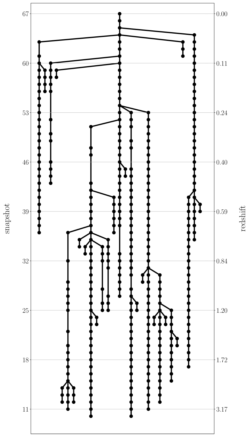
Figure 2: The merger tree of a main halo at redshift zero as found by ACACIA. This tree was extracted from a low resolution cosmological DMO simulation containing $64^{3}$ particles for illustrative purposes. Using higher resolutions quickly leads to hundreds and thousands of branches, resulting in a rather messy plot. On the $y$ axis, the snapshot numbers and their corresponding redshifts are given. The $x$ axis has no physical meaning. Each dot represents a clump identified at the given snapshot. Two dots connected by a vertical line represent clumps that have been linked as main progenitor and main descendant. Diagonal lines depict merging events. In this tree, a few links between two dots are larger than others. These are cases where clumps merge temporarily, but then re-emerge later as separate clumps (see the example shown in Figure 4). We discuss these cases and how they are dealt with in Section 3.3.

A straightforward method to link progenitors with descendants in two consecutive snapshots is to trace individual particles using their unique particle ID. All merger tree codes use this simple technique (Behroozi et al., 2013b; Springel et al., 2005a; Jiang et al., 2014; Knebe et al., 2010; Tweed et al., 2009; Elahi et al., 2019; Jung et al., 2014; Rodriguez-Gomez et al., 2015) with the notable exception of the code JMERGE described and tested in Srisawat et al. (2013).

Linking a progenitor to a descendant means checking how many particles of the progenitor halo or sub-halo end up in the descendant halo or sub-halo. Naturally, these tracer particles may end up in multiple clumps, giving multiple descendant candidates for a progenitor. In such cases, the most promising descendant candidate will be called the main descendant. To find a main progenitor and a main descendant, a merit function $\mathcal{M}$ has to be defined, which is to be maximised or minimised, depending on its definition. An overview of the merit functions that are used in other merger tree algorithms is given in Table 1 of Srisawat et al. (2013). The merit function used in our implementation is given in Equation 6.

Sometimes, unfortunately, linking progenitors to descendants is not as straightforward as described so far. We now discuss two circumstances where special care must be taken to define robust links between different snapshots: fragmentation events and temporary merger events.

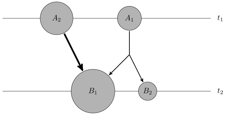
Figure 3: Illustration of a fragmentation event, where a progenitor $A_{1}$ at time $t_{1}$ is partially merged together with a second progenitor $A_{2}$ into a descendant $B_{1}$ at time $t_{2}>t_{1}$, while some fragmented part of $A_{1}$, $B_{2}$, evaded the merging.

3.2 Fragmentation Events

In our current approach, each progenitor can have only one descendant. We therefore need to pick only one descendant within a possibly large ranked list of descendant candidates, that all contain particles coming from the progenitor.

Normally, this choice is performed according to the ranking provided by the merit function, where the main descendant is ranked number 1. Problems arise for example when the progenitor $A_{1}$ is not the main progenitor of its main descendant $B_{1}$, but also has fragmented into another viable descendant candidate $B_{2}$. This situation is schematically shown in Figure 3.

Relying only on the merit function (6), progenitor $A_{1}$ will seem to have merged with $A_{2}$, the direct progenitor of $B_{1}$, in order to form $B_{1}$. The other fragment, $B_{2}$, will be treated as a newly formed clump and the entire formation history of $B_{2}$ would be lost. In order to preserve this history, we choose to prioritize the link from $A_{1}$ to $B_{2}$ over of merging progenitor $A_{1}$ into $B_{1}$.

It is simpler to deal with this case directly in the algorithm than via the merit function. The resulting logic can be summarized as follows: If $A_{1}$ is not the main progenitor of its main descendant $B_{2}$, then we don’t merge it into $B_{2}$ but we link it instead with the first secondary descendants that considers $A_{1}$ as its main progenitor.

3.3 Temporary Merger Events

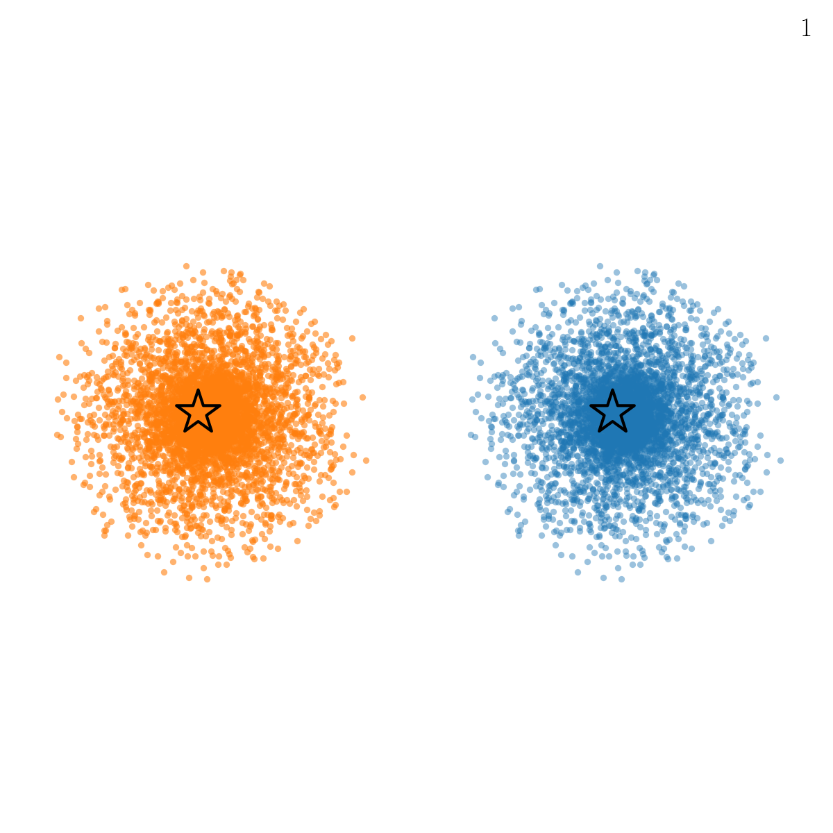
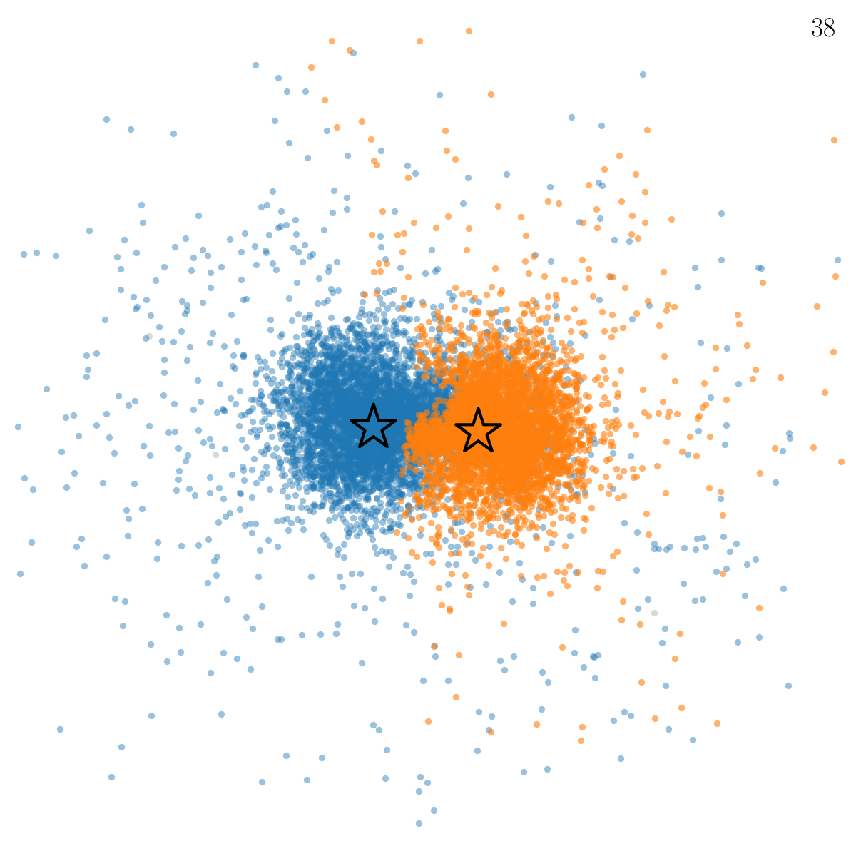
Figure 4: Illustration of how haloes can seemingly merge into another one and re-appear a few snapshots later. The blue and orange particles are two initially distinct haloes that pass through each other. The galaxies assigned to them are marked by a star with the same colour as the particles. Fully black stars mark orphan galaxies, which have lost their unique host (sub)halo. The number in the upper right corner of each plot is the snapshot number that is depicted. In snapshots 27-32, the halo-finding algorithm doesn’t identify both haloes as distinct objects. However by tracing the blue halo’s orphan galaxy it was possible to link the halo in snapshot 33 all the way back to snapshot 26.                                                                                                                                     The initial conditions were created using DICE (Perret, 2016).

When a sub-halo travels towards the core of its parent halo, it will merge with the central clump and disappear from the sub-halo lists. It can however re-emerge at a later snapshot and will be added back to the list as a newly born halo. Such a scenario is shown in Figure 4. Indeed, when this occurs, the merger tree code will deem the sub-halo to have merged into the main halo, and will likely find no progenitor for the re-emerged sub-halo, thus treating it as newly formed.

This is a problematic case because we lose track of the growth history of the sub-halo, regardless of its size, and massive clumps may be found to just appear out of nowhere in the simulation. This is a well known problem for configuration-space halo finders (Onions et al., 2012), and phase-space halo finders like ROCKSTAR (Behroozi et al., 2013a) have been developed precisely to alleviate this issue. While they typically perform better than configuration-space halo finders, Srisawat et al. (2013) found that phase-space halo finders aren’t infallible in recovering all such missing haloes, and strongly recommend checking for links between progenitors and descendants in non-consecutive snapshots as well.

As our merger tree code works on the fly, future snapshots will not be available at the time of the merger tree analysis, so it will be necessary to check for progenitors of a descendant across multiple snapshots. This can be achieved by keeping track of the most bound particles of each clump when it is merged into some other clump. These tracer particles are also used to track orphan galaxies. For this reason, we call these tracer particles “orphan particles”, and progenitor-descendant links over non-adjacent snapshots “jumpers”.

These jumper links between different haloes widely separated in time are less reliable than proper links between progenitors and descendants from adjacent snapshots. As we will discuss in Section 5.3, the quality of the merger trees increases with the number of tracer particles used. Using jumpers corresponds to using only one tracer particle over a large time interval, much larger than the one between two adjacent snapshots.

For this reason, priority is given to direct progenitor candidates in adjacent snapshots. Only if no direct progenitor candidates have been found for some descendant, then progenitor candidates from non-adjacent snapshots are searched for. Because these progenitors from non-adjacent snapshots are only tracked by one single particle, we don’t use the merit function to rank them. Instead, we find the orphan particle within the descendant clump which is the most tightly bound.

In conclusion, although not ideal, using jumpers remains a necessity to track these temporary merger events. As a bonus, it allows us to track orphan galaxies as will be discussed in Section 6.

4 Details Of Our New Algorithm

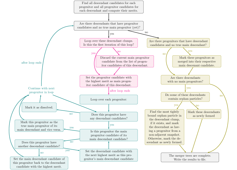
Figure 5: Flowchart of the tree making algorithm. For more details, please refer to Section 4 in the main text.

For clarity, the algorithm that we describe in what follows is also shown in a flow diagram in Figure 5. The first step of our algorithm is to identify plausible progenitor candidates for descendant clumps, as well as descendant candidates for progenitor clumps. We achieve this by tracking tracer particles across simulation snapshots. For any given snapshot, the tracer particles of each clump are selected within the list of all particles belonging to the clump, ranked from most bound to least bound. Indeed, the most bound particles are expected to remain well within the clump boundary between two snapshots. The main parameter of our method is the maximum number of these tracer particle used per progenitor clump, called $n_{\rm mb}$. The minimum number of tracer particles is obviously equal to $n_{\rm min}$, the minimum mass threshold in units of particle masses adopted by the PHEW clump finder.

So for every clump in the current snapshot, the $n_{\rm mb}$ most bound tracer particles are found and written to file. In the following output step, those files are read in and the tracer particles are used to determine which clumps of the previous snapshot are the progenitor candidates of the clumps of the current snapshot. For each progenitor clump, we compile a list of descendant clump candidates by finding all descendant clumps which contain tracer particles of said progenitor. Conversely, we also compile a list of progenitor candidates for each descendant clump by finding all tracer particles amongst the descendant clump’s particles and by noting which progenitor clump they are tracing.

As explained earlier, in order to generate the merger trees the main progenitor of each descendant and the main descendant of each progenitor need to be found. Commonly at this point however, multiple progenitor candidates have been found for every descendant, as well as multiple descendant candidates for each progenitor. Therefore, we somehow need to select the “best” candidate amongst those with the aim of generating reliable merger trees. To be able to select the “best”, we first quantify how “good” a candidate is by assigning a merit to each descendant candidate of every progenitor, as well as every progenitor candidate of each descendant. We define the merit as follows:

Let $\mathcal{M}_{\rm pd}(A,B_{i})$ be the merit function to be maximised for a list of descendant candidates $B_{i}$ of a progenitor $A$. Let $n_{\rm mb}$ be the total number of particles of progenitor $A$ that are being traced. Note that $n_{\rm mb}$ can be smaller than the total number of particles in clump $A$. A straightforward ansatz for the merit function would be to based on the fraction of particle traced from the progenitor to the descendant candidate:

$$\mathcal{M}_{\rm pd}(A,B_{i})\propto\frac{n_{A\cap B_{i}}}{n_{\rm mb}}$$ (3)

where $n_{A\cap B_{i}}$ is the number of tracer particles of $A$ found in $B$. Similarly, we define $\mathcal{M}_{\rm dp}(A_{i},B)$ as the merit function to be maximised for a list of progenitor candidates $A_{i}$ of a descendant $B$. Another straightforward ansatz would be based on the fraction of particle traced from the progenitor candidates to the descendant:

$$\mathcal{M}_{\rm dp}(A_{i},B)\propto\frac{n_{A_{i}\cap B}}{n_{B}}$$ (4)

where $n_{B}$ is the total number of particles in the descendant $B$. In these two merit functions, $n_{\rm mb}$ and $n_{B}$ are just normalizing factors. They are independent of the properties of the candidate and hence won’t affect the selection process. We can therefore define a generic merit function as

$$\mathcal{M}(A,B)\propto n_{A\cap B}$$ (5)

The PHEW clump finder in RAMSES identifies the main halo as the clump with the highest density maximum. During a major merger event, the halo will have two clumps with similar masses and comparable maximum densities. It is then quite common that small variations in the value of the density maxima will cause the identification of the main halo to jump between these two clumps. Indeed, the particle unbinding algorithm will identify particles that are not bound to the sub-halo and pass them on to the main halo, modifying the resulting mass for the two clumps. This effect is particularly strong if one uses the strictly bound definition for the particle assignment. As a consequence, because the identification of the main halo varies, strong mass oscillations are expected. To counter this spurious effect, we modify the merit function to preferentially select candidates with similar masses:

$$\mathcal{M}(A,B)=\frac{n_{A\cap B}}{n_{\rm max}-n_{\rm min}}$$ (6)

where $n_{\rm max}=\max(n_{A},n_{B})$ and $n_{\rm min}=\min(n_{A},n_{B})$. An overview of other merit functions used in the literature is given in Table 1 of Srisawat et al. (2013).

With the merit function defined, let’s return to the tree making algorithm. We left off with the commonly encountered situation in which we have identified multiple progenitor candidates for descendants and vice versa, and are now looking to find a matching progenitor-descendant pair, where the main progenitor candidate of a descendant has precisely this descendant as its main descendant candidate. This search is performed iteratively. At every iteration, we first look at all progenitors that haven’t found their respective match yet, and check all of their descendant candidates for a match. The loop over descendant candidates for a given progenitor is performed in order of decreasing merit of the descendant candidates, and the checks are stopped either when a progenitor has found a match, or has run out of candidates. (In case a progenitor has no descendant candidates at all, we consider it as dissolved.) Once all the progenitors have been checked, the second step of the iteration begins. We now look at all descendants that haven’t found their respective match yet. For these descendants, we discard the current, unsuccessful main progenitor candidate in favour of the progenitor candidate with the next highest merit, and the first step of the iteration begins anew: All progenitors without a matching main descendant again loop over all their descendant candidates in search for a match. This two-step iteration is repeated until either all descendants have found their match, or have run out of progenitor candidates.

After the iteration finishes, we may have both progenitors as well as descendants which aren’t part of a matching pair. We deal with them as follows:

1. Progenitors that have not found any available descendant will be considered to have merged into the descendant candidate with the highest merit. These progenitors are recorded in the merger tree as merged progenitors. In this case, only one tracer particle is kept for future use, the most strongly bound particle in the list of $n_{\rm mb}$ tracer particles. This single particle is referred to as the orphan particle of the merged progenitor. It is used to check whether the merger event was a final merger or only a temporary merger. It is also used to track orphan galaxies.

2. Descendants that have not found any available progenitor will be checked against non-consecutive past snapshots. The particles of the descendant are compared to the orphan particles in the list of past merged progenitors. The most strongly bound orphan particle will be used to restore the broken link with its main progenitor. Finally, remaining descendants without a progenitor are considered as being newly formed.

Finally, we note that the choice to first check all progenitor candidates of descendants and only merge progenitors into descendants later is how we deal with fragmentation events (see Section 3.2) in an attempt to preserve the formation history of clumps. Effectively, this procedure assigns more weight to a descendant having progenitor candidates at all over the merging of a progenitor into its main descendant candidate, as the merit function would suggest.

5 Testing and Optimizing the Algorithm

The current implementation of our merger tree algorithm needs several free parameters to be chosen by the user. We present in this section multiple tests that reveal the recommended values for these parameters. We use for this a single reference cosmological simulation and analyze the merger trees we obtained for different set of parameters. A similar methodology was used in the Sussing Merger Trees Comparison Project (Srisawat et al., 2013; Wang et al., 2016; Avila et al., 2014; Lee et al., 2014). This is why we adopt in this section several tests from this seminal work, as they are quite efficient at testing the strengths and the weaknesses of merger tree codes. They also allow for a direct comparison of our new implementation with many other state-of-the-art merger tree codes in the community.

5.1 Test Suite

We now list the different diagnostics we use to characterize the quality of our merger tree algorithm.

1. Length of the Main Branch of a Halo

   The length of the main branch of a halo is simply defined as the number of snapshots in which a halo and all its progenitors are detected. A halo at $z=0$ without any progenitors will be considered as newly formed and thus will have a main branch of length $1$. If a halo appears to merge temporarily into another and re-emerges at a later snapshot, the missing snapshots will be counted towards the length of the main branch as if they weren’t missing. Traditionally, finding long main branches is considered as a good thing for a merger tree code.

2. Number of Branches of a Halo

   Another popular quantity is the number of branches of the tree leading to the formation of a halo at $z=0$. The main branch is included in this count, thus the minimal number of branches is $1$. If a different choice of parameters leads to a reduction of the number of branches, it usually corresponds to an increase of the average length of the main branches and a smaller number of merger events. For example, intuitively if we compare the merger trees where we use only one tracer particle per clump to the trees that were built using several hundreds tracer particles per clump, we would expect to be able to detect more fragmentation events with the increased number of tracer particles. If the fragmentation remained undetected, we would instead have found a newly formed clump (the fragment) alongside a merging event. Both the “newly formed” fragment as well as its progenitor, which is now merged into a descendant, will have shorter main branches. Conversely, the descendant will have an increased number of branches compared to the scenario where the fragmentation was detected. Finally, in the hierarchical picture of structure formation, one would expect more massive clumps to have longer main branches and a higher number of branches.

3. Logarithmic Mass Growth of a Halo

   The logarithmic mass growth rate of a halo is computed using the following finite difference approximation:

   $$\frac{\mathrm{d}\log M}{\mathrm{d}\log t}\simeq\frac{(t_{k+1}+t_{k})(M_{k+1}-M_{k})}{(t_{k+1}-t_{k})(M_{k+1}+M_{k})}\equiv\alpha_{M}(k,k+1)$$ (7)

   where $k$ and $k+1$ are two consecutive snapshots, with the corresponding halo mass $M_{k}$ and $M_{k+1}$ and times $t_{k}$ and $t_{k+1}$. A convenient approach was proposed by Wang et al. (2016) to reduce the range of values to the interval $(-1,1)$ using the new variable

   $$\beta_{M}=\frac{2}{\pi}\arctan(\alpha_{M})$$ (8)

   Note that we expect the mass of dark matter haloes to increase systematically with time. We also expect in some cases the mass to remain constant or even to decrease slightly. We nevertheless expect the distribution of $\beta_{M}$ to be skewed towards $\beta_{M}>0$. $\beta_{M}\rightarrow\pm 1$ imply $\alpha_{M}\rightarrow\pm\infty$, indicating suspiciously extreme cases of mass growth or mass loss.

4. Mass Growth Fluctuation of a Halo

   Mass growth fluctuations are defined similarly as

   $$\xi_{M}=\frac{\beta_{M}(k,k+1)-\beta_{M}(k-1,k)}{2}$$ (9)

   where $k-1$, $k$, $k+1$ are three consecutive snapshots. A smooth mass accretion history generally leads to $\xi_{M}\simeq 0$. Strong deviations from zero could indicate an erratic behaviour, indicating extreme mass loss followed by extreme mass growth and vice versa. Within the standard model of structure formation, this behaviour is expected only during major merger events. Otherwise, it might indicate either a misidentification by the merger tree code or a misdetection by the halo finder.

Ideally, we should have tested ACACIA on the dataset used in Srisawat et al. (2013) and Avila et al. (2014) (S13 and A14 from here on, respectively). This would have enabled a direct comparison of the performance to other merger tree codes. However, ACACIA was designed to work on the fly with the RAMSES code. Using it as a post-processing tool would defeat its purpose and as a matter of fact handling other halo catalogues has proven technically impossible. ACACIA is tightly coupled to the PHEW halo finder, and relies heavily on already existing internal structures and tools, in particular the explicit communications which are necessary for parallelism on distributed memory architectures, as well as the structures and their hierarchies as they are defined by PHEW. Attempting to use other halo catalogues would require us to re-write a significant portion of the PHEW halo finder. If we instead used only particle data, which is possible, we would still find a different halo catalogue compared to other structure finding codes, and we would still not be able to do an exact comparison. Furthermore, we also want to demonstrate that the PHEW halo finder can be used within the RAMSES code to produce reliable merger trees. For these various reasons, we have decided to perform the same tests but using our own dataset generated on the fly by RAMSES.

Despite this limitation, we have performed a direct comparison to other halo finders and merger tree codes using the exact same merger tree parameters as in A14. The results are given in Appendix A. Our results are comparable to e.g. the MergerTree, TreeMaker and VELOCIraptor tree builders with AHF, Subfind, or Rockstar halo finders as presented in A14, demonstrating that ACACIA performs similarly than other state-of-the-art tools.

In this section, we would like to explore different parameters and see how they affect the quality of the merger tree. Our tests are performed on a single DMO simulation with $256^{3}\approx 1.7\times 10^{7}$ particles of identical mass $m_{p}=1.6\times 10^{9}M_{\sun}$. To enable a comparison with A14, we adapted the same cosmology and snapshot output times as them at a comparable, but slightly lower resolution. The cosmological parameters used are taken from the WMAP-7 (Komatsu et al., 2011), while the snapshot times are identical to the ones used for Millenium Simulation (Springel et al., 2005b), starting at redshift 50 and being roughly uniformly spaced in log $a$ in 61 steps. At redshift zero, the simulation was then continued for 3 further snapshots to ensure that the merging events at $z=0$ are actual mergers and not temporary mergers that will re-emerge later.

This choice of spacings between the snapshots was relatively arbitrarily in the sense that we did not take into account any further underlying physical considerations that would be important in e.g. semi-analytical models. For different snapshot spacings, we recommend to follow the suggestions found by Wang et al. (2016):

• Sequences of snapshots with very rapidly changing time intervals between them should be avoided as they can lead to very poor trees.

• Increasing the number of outputs from which the tree is generated results in shorter trees. This is because, due to limitations in the input halo catalogue, tree-builders may face difficulties caused by the fluctuating center and size of the input haloes, and the frequency of detected temporary merging events increases with the number of snapshots, resulting in haloes missing from the catalogue. For merger trees built from an order of 100 or more snapshots, they recommend using an algorithm capable of dealing with these problems, which ACACIA is able to do, although at the moment this patching of missing haloes in the catalogue isn’t based on a physical timescale, but on a user defined number of snapshots.

• To facilitate this patching at the end of the simulation, snapshots should be generated beyond the desired endpoint. This would entail typically running past $z=0$, as we did with our test suite.

For the clump finder, we have adopted a outer density threshold of 80$\bar{\rho}$ and a saddle surface density threshold of 200$\bar{\rho}$, where $\bar{\rho}=\Omega_{m}\frac{3H^{2}}{8\pi G}$ is the average density. The minimal mass for clumps is set to 10 particles. Note that for the histogram of the logarithmic mass growth and mass growth fluctuations, we adopt a threshold for the clump mass of 200 particles for sake of visibility. Choosing a smaller mass threshold would indeed give too much weight to small mass, poorly resolved haloes in our statistical analysis.

5.2 Varying the Clump Mass Definition

In our current implementation, there are two important parameters that can have a strong effect on the halo catalogue (beside the mass and the density thresholds mentioned earlier) and the corresponding merger tree.

The first one is the exact definition adopted for the mass of the sub-haloes in the merit function. For main haloes, there is no ambiguity as the mass is defined as the sum of the masses of all particles contained within the boundary of the halo (set by the outer density isosurface). This is not the case for sub-haloes, because of the unbinding process described in Section 2. Indeed, unbound particles are removed from their original sub-halo and passed to the parent sub-halo in the hierarchy. Clump masses are therefore defined as the sum of the mass of all bound particles. In the merit function evaluation, we however consider two different cases to compute the mass: 1- the mass is equal to the sum of the masses of only the bound particles, like for sub-haloes or 2- the mass is equal to the sum of the masses of all particles within their boundaries (set by the saddle surface with neighbouring clumps), like for main haloes. In the former case, the mass used in the merit function is identical to the clump mass. It is referred to as the exclusive case. In the latter case, the mass in the merit function is different that the sub-halo mass definition but identical to the main halo mass definition. We refer to this case as inclusive.

The second important definition is the exact boundedness criterion adopted for the unbinding process. As discussed in Section 2, we explored two different cases: When particles are allowed to leave the outer boundary of their host clump (and possibly come back later) or when particles are not allowed to cross the saddle surface during their orbital evolution. In the first case, we only require the binding energy to be negative, while in the second case, the binding energy has to be smaller than the gravitational potential of the nearest saddle point. We call the first case loosely bound and the second case strictly bound.

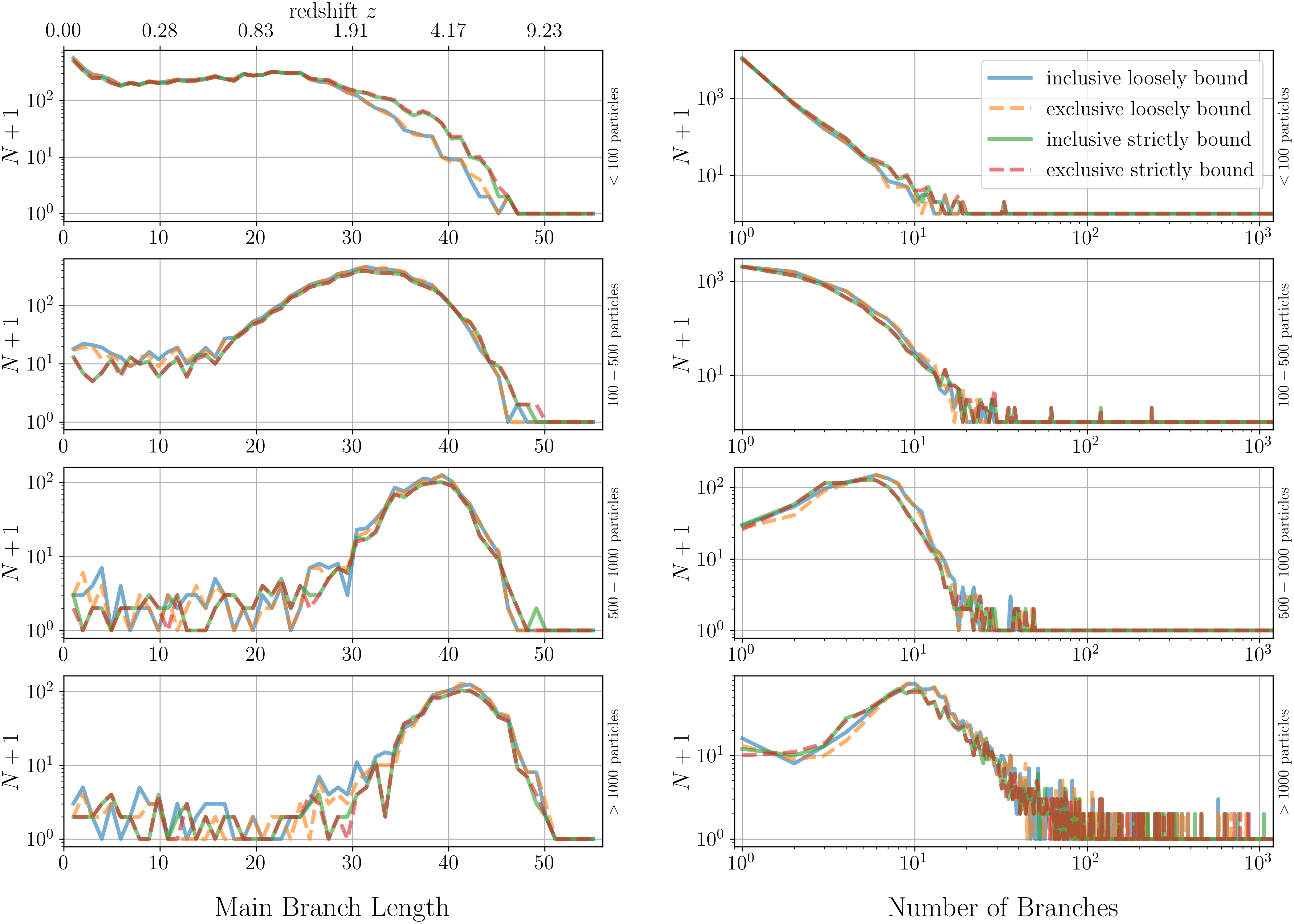
Figure 6: Histogram of the length of main branch (left) and of the number of branches (right) for all clumps (halo and sub-halo) detected at $z=0$. Each row corresponds to a different range of clump masses (expressed in particle numbers): less then 100 (top), 100-500, 500-1000 and more than 1000 (bottom). We compare these histograms for four different cases: whether unbound particles are included (inclusive) or excluded (exclusive) in the evaluation of the merit function, and whether bound particles are loosely bound or strictly bound.

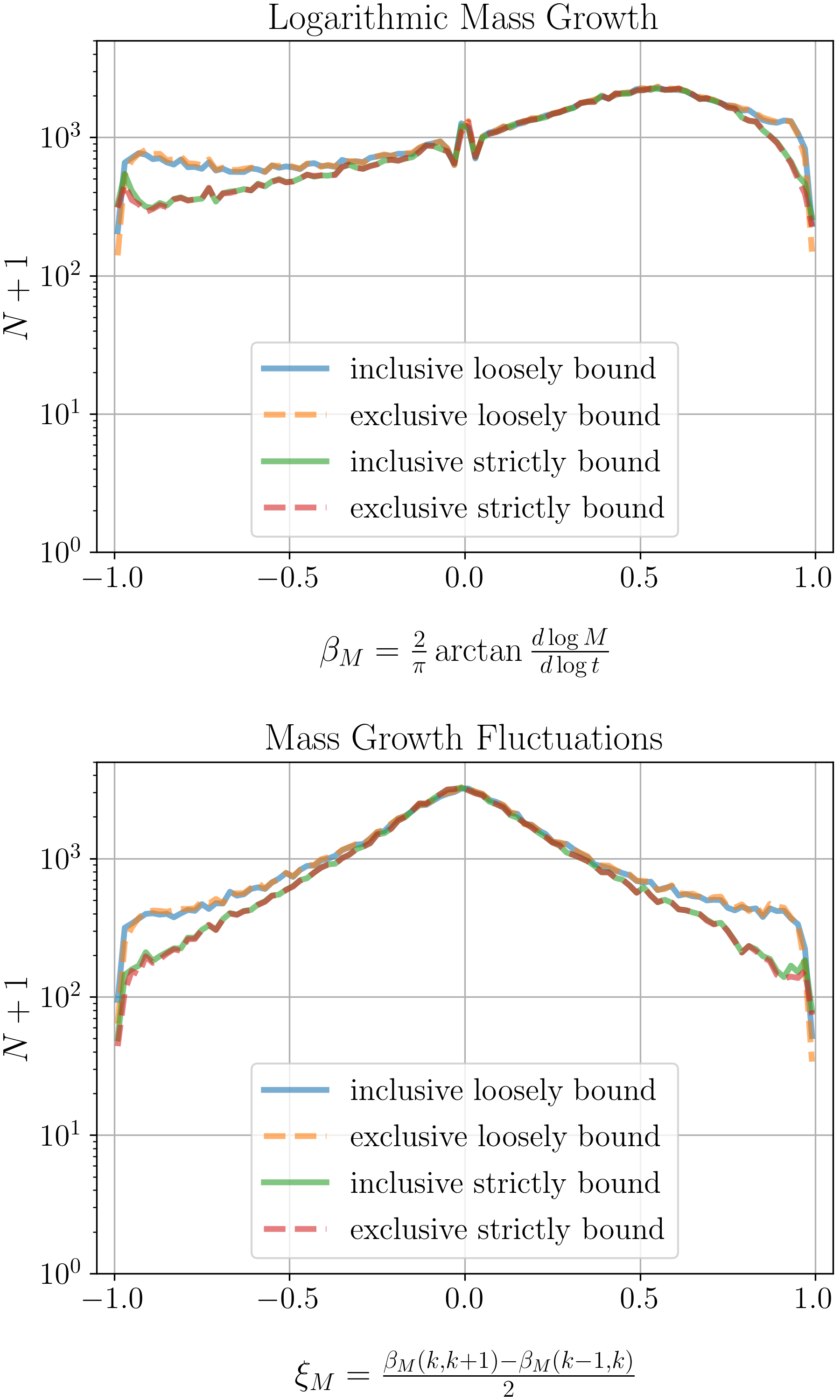
Figure 7: Histogram of the logarithmic mass growth (top) and the mass growth fluctuation (bottom) for all clumps (halo and sub-halo) detected in two (top) or three (bottom) consecutive snapshots of the simulation and with more than 200 particles. We compare these histograms for four different cases: whether unbound particles are included (inclusive) or excluded (exclusive) in the evaluation of the merit function, and whether bound particles are loosely bound or strictly bound.

Table 2: Average data for all clumps at $z=0$ depending on whether to consider particles which might wander off into another clump as bound (loosely bound) or not (strictly bound). The results shown are for the exclusive mass definition, which show no significant difference to when the inclusive mass definition is used.

	strictly bound	loosely bound
total clumps	17115	18247
median number of particles in a clump	77	85
average main branch length
clumps with < 100 particles	14.7	13.0
clumps with 100-500 particles	31.4	31.0
clumps with 500-1000 particles	37.5	37.3
clumps with > 1000 particles	40.7	40.9
average number of branches
clumps with < 100 particles	1.2	1.1
clumps with 100-500 particles	2.8	2.8
clumps with 500-1000 particles	6.2	6.7
clumps with > 1000 particles	25.4	26.1

We now test our algorithm with these four different options for the clump masses, using the simulation presented in the previous section. Note that we used here $n_{\rm mb}=200$ tracer particles to identify links in the merger tree. We will study the impact of this other important parameter in the next section.

We show in Figure 6 the histogram of the length of the main branch and the histogram of the number of branches for each clump (halo and sub-halo) at $z=0$ and for each of our four different mass definitions. In all four cases, we see that more massive clumps tend to have longer main branches and a higher number of branches. This is also visible from the average length of the main branch and the average number of branches in different bins of halo masses given in Table 2. This is a well-known property of cosmological simulations in the hierarchical scenario of structure formation.

Whether clump masses are defined in an exclusive manner (like for sub-haloes) or in an inclusive manner (like for main haloes) in the merit function has negligible effect on these two statistics. This means that this a priori large difference in the mass definition of the merit function has no effect on the linking process of the merger tree. The distinction between strictly bound and loosely bound particles does not change much for larger clumps but does change the length of the main branch (and to a lesser extent the number of branches) for small mass clumps (less than 100 particles). Our first idea was that strictly bound particles might be better at identifying robust links between snapshots. It turned out that the main effect of changing the mass definition from loosely bound to strictly bound is to reduce the mass of the clump and to promote them systematically from a larger mass bin to a smaller mass bin. We see indeed in Figure 6 and Table 2 that the number of clumps is reduced in the large mass bins and increased in the smallest mass bin, explaining that this change in the mass definition merely transfers clumps between different bins and affects the statistics accordingly.

A qualitative comparison of the length of the main branches of the most massive haloes that we obtain in Figure 6 to Figure 3 of A14 shows that our results are in good agreement with what the other codes find: The distribution peaks around the length of 45, it is about 20 snapshots wide, and there are only few cases with main branch lengths below 30. This is in good agreement with what e.g. the MergerTree, TreeMaker, and VELOCIraptor tree builders find in combination with the Rockstar or Subfind halo finders. We note that in Figure 3 of A14, both the peak of the distribution and the maximal value of the main branch lengths they found are at slightly higher values than ours. We attribute this to the slightly lower resolution of our simulations: The first identifiable clumps we find are at snapshot 10, leading to a maximal main branch length of 51, compared to $\sim 53$ that A14 find. Compared to Figure 3 of S13, the distributions we find for the lower mass clumps are also in very good agreement. Our high clump mass distribution however is much narrower around the peak value of $\sim 45$. This difference is due to the different halo finders employed, as is demonstrated in Figure 3 of A14. The AHF halo finder, which was used in S13, displays the same differences in the distribution of main branch lengths for nearly all tree codes.

We also note in Figure 6 that a few large clumps (with mass larger than 500 particles) at $z=0$ have a main branch length of unity. These large clumps don’t have any progenitor and thus essentially appeared out of nowhere. As explained in S13, this effect is present in many state-of-the-art merger tree codes and is due to fragmentation events at the periphery of large haloes leading to a misidentification of a few rare progenitor-descendant links. We have however identified a second culprit, which is the way that PHEW establishes substructure hierarchies and the subsequent particle unbinding. The hierarchy is determined by the density of the density peak of each clump: A clump with a lower peak density will be considered lower in the hierarchy of substructure. So in situations where two adjacent clumps have similarly high density peaks, their order in the hierarchy might swap. The unbinding algorithm then strips the particles from the sub-haloes that have the lowest level in the hierarchy and passes it on to the next level, amplifying the particle loss which these sub-haloes experience. This loss of particles is essential here because it prevents the algorithm to establish links between progenitors and descendants. About half of the main branches that we tracked back in time were cut short for this reason: The leaf of the main branch was a sub-halo with much fewer particles ($\sim 100$) whose progenitor the algorithm was not able to identify and who in subsequent snapshots was found to be the main halo, gaining a lot of mass in a very short time. So this issue arises due to the halo finder, not due to the tree builder.

The histogram of the logarithmic mass growth shown in Figure 7 is indeed skewed towards $\beta_{M}>0$, demonstrating that clump masses are on average growing. Based on the shoulder of the histogram around $\beta_{M}\sim 0.6$ our results are comparable to those of the HBThalo and Subfind halo finders in Column A of Figure 8 of A14 for all tree codes. We do find more extreme events with $\beta_{M}\rightarrow\pm 1$, which are due to the smaller mass haloes and sub-haloes that we used compared to A14. Indeed, when we apply the appropriate mass thresholds in Appendix A, these extreme events are significantly reduced. The small wiggle around $\beta_{M}=0$ is due to the discrete particle masses and the linear binning of the histogram. Adopting a merit function based on the inclusive or exclusive mass definition has here also no effect on the mass growth and mass growth fluctuation statistics. At first sight, using the strictly bound instead of the loosely bound definition would have led to more robust links and a smoother mass growth. In Figure 7, we do see in the latter case more extreme mass growth around $\beta_{M}\rightarrow\pm 1$ and mass growth fluctuations around $\xi_{M}\rightarrow\pm 1$. We verified that the increase in the number of these extreme events for the loosely bound case is in fact due to a larger number of small sub-haloes that satisfy the adopted mass threshold of 200 particles. This just means that mass growth statistics is more robust for large, well resolved haloes, while smaller clumps, closer to the resolution limit (between 10 and 100 particles; see discussion below) are less reliable.

In conclusion, whether to use inclusive or exclusive mass definitions in the merit function has no effect on the final merger trees, while using a strictly bound definition for the clump mass is preferable. We expected the strictly bound clumps to allow more stable tracking, but the only effect we noticed was that it systematically promotes sub-haloes to lower masses and so naturally selects better resolved, higher mass clumps from the halo catalogue.

5.3 Varying the Number of Tracer Particles

Table 3: Average length of main branch and average number of branches for clumps in different mass bins at $z=0$ and for varying numbers of clump tracer particles $n_{\rm mb}$.

$n_{\rm mb}=$	1	10	50	100	200	500	1000
Average main branch length
clumps with < 100 particles	24.2	24.3	23.6	23.4	23.2	22.9	22.7
clumps with 100-500 particles	50.4	50.1	49.5	49.1	48.8	48.8	48.8
clumps with 500-1000 particles	55.2	54.9	53.3	54.1	54.7	54.3	54.2
clumps with > 1000 particles	56.7	54.9	52.3	52.9	54.0	55.8	56.4
Average number of branches
clumps with < 100 particles	1.2	1.3	1.3	1.3	1.3	1.4	1.4
clumps with 100-500 particles	2.7	3.0	3.3	3.3	3.4	3.6	3.6
clumps with 500-1000 particles	6.6	7.2	8.1	8.2	8.7	8.9	9.1
clumps with > 1000 particles	20.4	25.2	27.3	28.6	29.5	30.4	31.4

Table 4: Number of dead trees pruned from the merger tree catalogue for varying numbers of tracer particles $n_{\rm mb}$ throughout all snapshots. “LIDIT” is an abbreviation for “last identifiable descendant in tree”. For a LIDIT, no descendant could have been identified throughout the simulation and consequently the corresponding tree is considered dead and pruned from the merger tree catalogue. LIDITS are obviously a spurious feature of the merger tree algorithm.

$n_{\rm mb}=$	1	10	50	100	200	500	1000
dead trees pruned from tree catalogue	23617	15438	14467	14433	14432	14432	14433
highest particle number of a LIDIT	6418	674	182	182	182	182	182
median particle number of a LIDIT	19	20	20	20	20	20	20
LIDITs with >100 particles pruned	493	61	32	28	26	26	26

Table 5: Number of “jumpers” (progenitor-descendant links found across non-adjacent snapshots) during the entire simulation for varying number of tracer particles $n_{\rm mb}$.

$n_{\rm mb}=$	1	10	50	100	200	500	1000
Total Jumpers	14738	15500	17654	18995	20505	20305	20407
Jumper Progenitors
clumps with < 100 particles	13372	14064	15696	16448	17233	16795	16779
clumps with 100- 500 particles	1295	1353	1833	2383	3024	3153	3214
clumps with 500-1000 particles	52	60	87	121	176	251	278
clumps with > 1000 particles	19	23	38	43	72	106	136

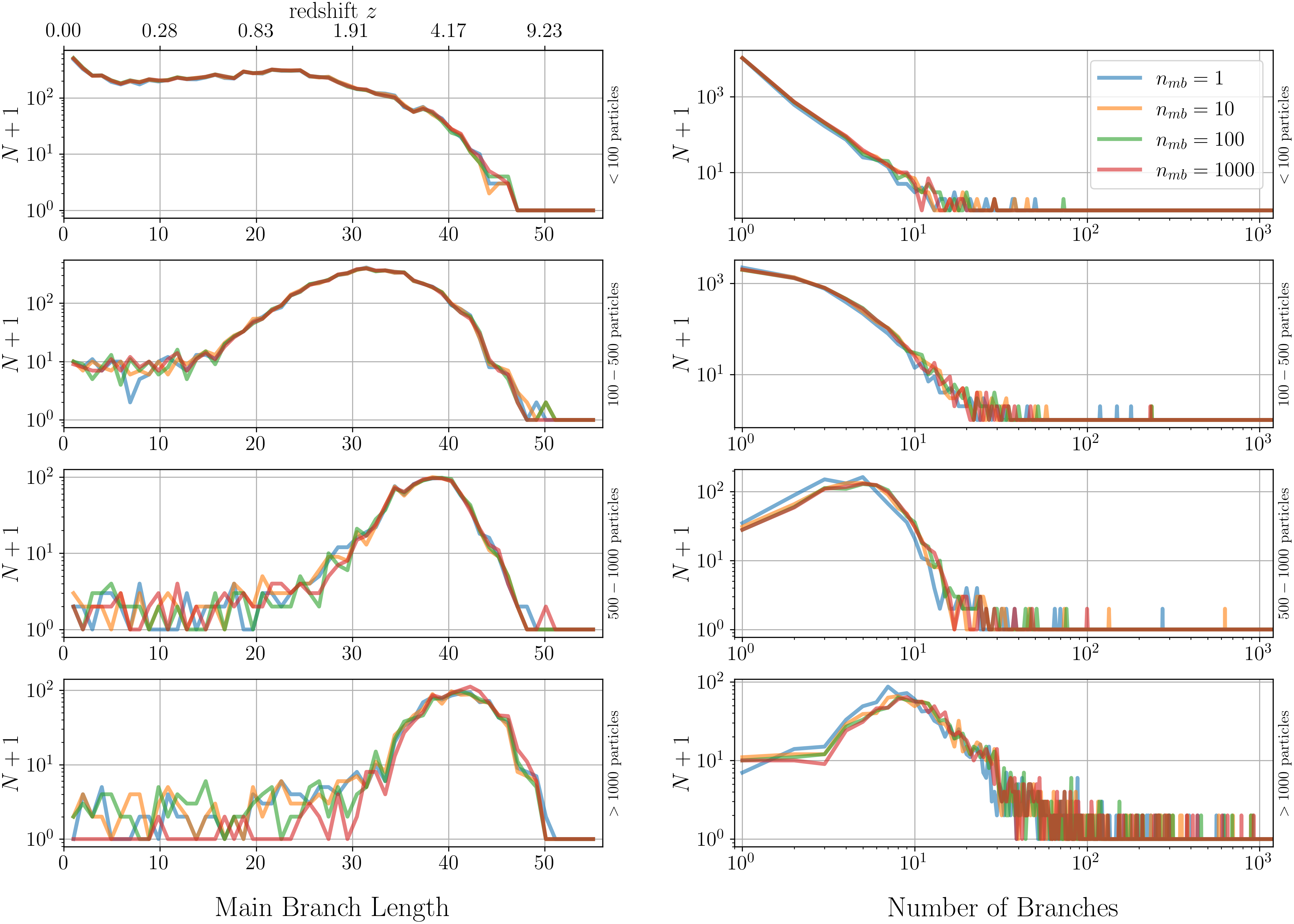
Figure 8: Histogram of the length of the main branch (left) and histogram of the number of branches (right) for all clumps (haloes and sub-haloes) detected at $z=0$ for different numbers of tracer particles $n_{\rm mb}$ indicated in the legend. Each row corresponds to a different range of clump masses (expressed in particle numbers): less then 100 (top), 100-500, 500-1000 and more than 1000 (bottom). In all cases, we used the exclusive and strictly bound clump mass definitions.

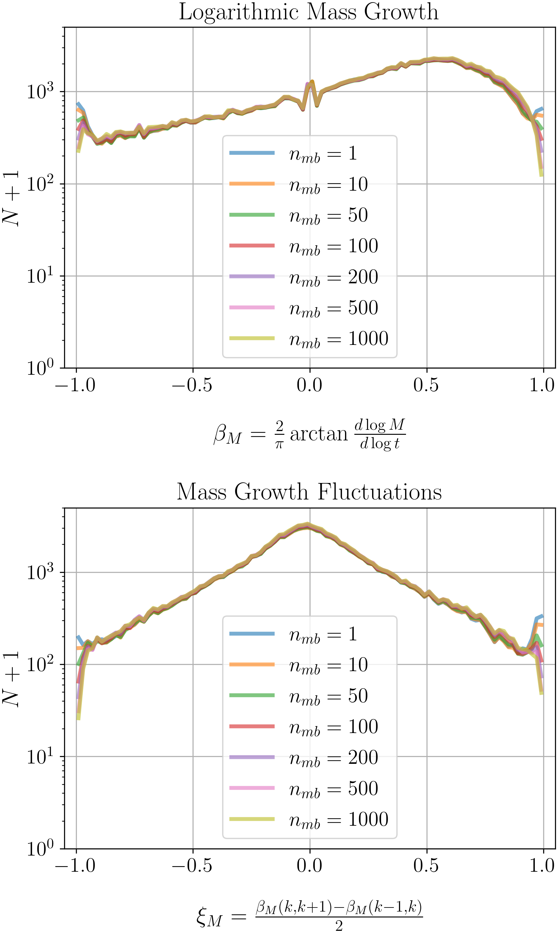
Figure 9: Histogram of the logarithmic mass growth (top) and histogram of the mass growth fluctuation (bottom) for all clumps (halo and sub-halo) detected in two (top) or three (bottom) consecutive snapshots of the simulation and with more than 200 particles. We compare these histograms for four different numbers of tracer particles $n_{\rm mb}$ as indicated in the legend. In all cases, we used the exclusive and strictly bound clump mass definitions.

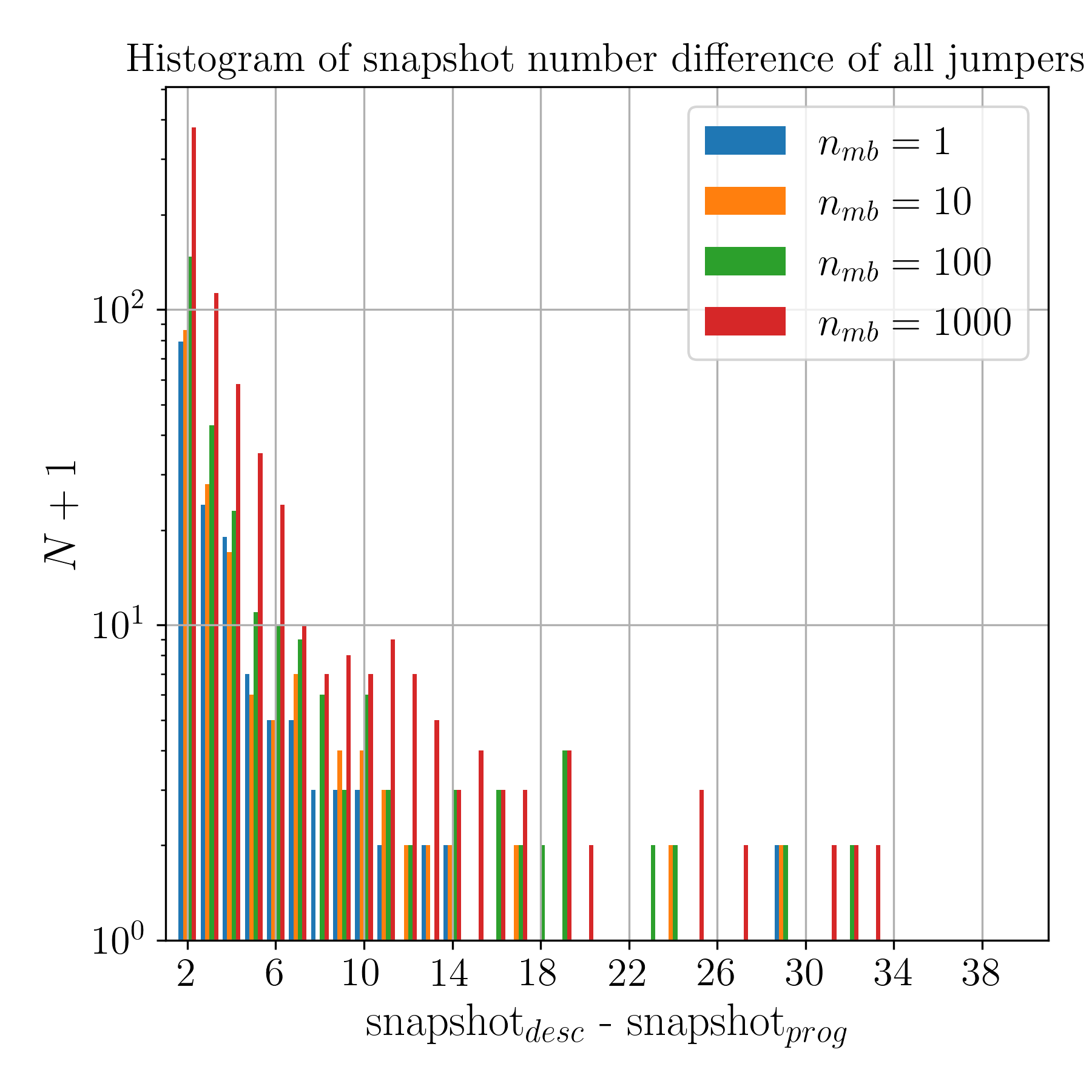
Figure 10: Histogram of the difference in snapshot numbers for jumpers, i.e. progenitor-descendant links which are made across non-adjacent snapshots. Only pairs where both the progenitor’s and the descendant’s masses exceed 200 particle masses were included in this plot. We compare these histograms for four different numbers of tracer particles $n_{\rm mb}$ as indicated in the legend. In all cases, we used the exclusive and strictly bound clump mass definitions.

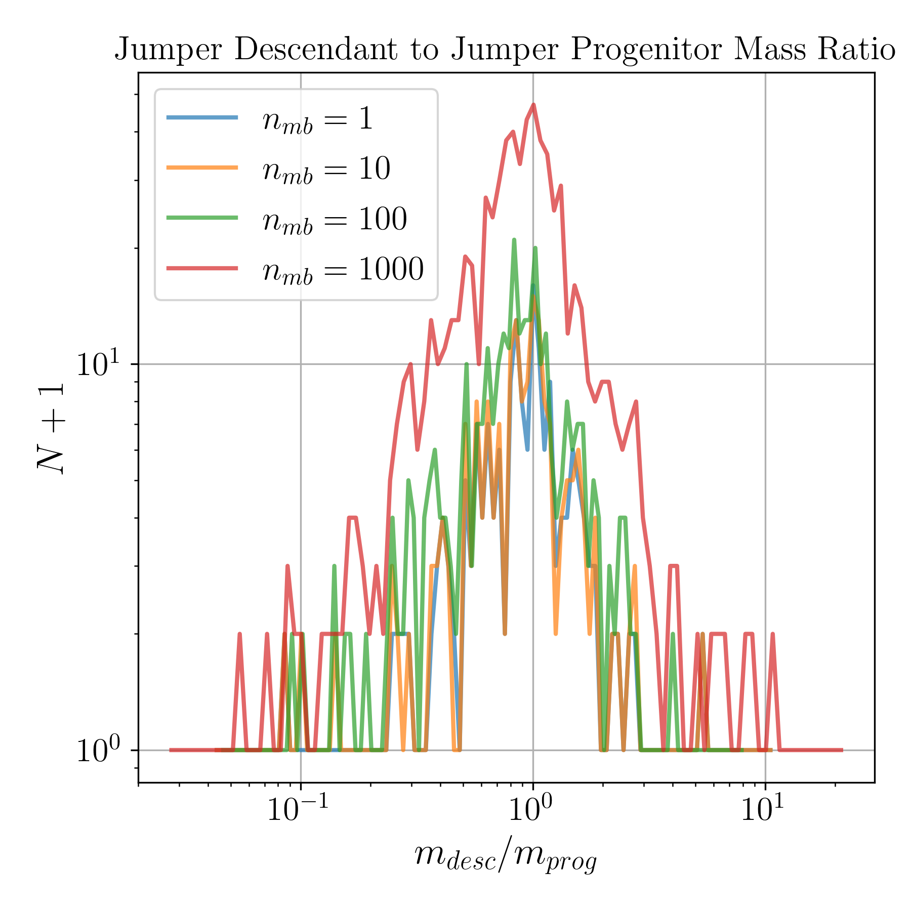
Figure 11: Histogram of the ratio of descendant mass to progenitor mass for jumpers, i.e. progenitor-descendant links which are made across non-adjacent snapshots. Only pairs where both the progenitor’s and the descendant’s masses exceed 200 particle masses were included in this plot. We compare these histograms for four different numbers of tracer particles $n_{\rm mb}$ as indicated in the legend. In all cases, we used the exclusive and strictly bound clump mass definitions.

In this section, we study the effect of varying the number of tracer particles on our various diagnostics of tree quality. Even though we performed the simulations with up to 1000 tracer particles, the mass threshold for clumps was always kept constant at 10 particles. The number of tracer particles per clump is an upper limit, not a lower limit. For clumps that contain less than $n_{\rm mb}$, this means that they will be traced by every single particle they consist of. In effect, we expect that this assigns greater weight to clumps which are more massive than $n_{\rm mb}$ to be identified as the main progenitor, and should hopefully decrease extreme mass growths and mass fluctuations. To illustrate, consider for example the merging of two clumps with unequal masses, where all of the tracer particles of both clumps are found inside the resulting merged descendant. Raising the number of tracer particles above the less massive clump’s particle number in this scenario means that the number of its tracer particles inside the descendant will remain constant, while the number of tracer particles stemming from the more massive clump will increase, and thus raising its merit to be the main progenitor. This is also the desired outcome. Should however both clumps have masses above $n_{\rm mb}$ particle masses, then our inclusion of the clump masses in the merit function should nevertheless find the more massive clump to be the main progenitor if it had a mass closer to the resulting descendants mass. So we expect that increasing the number of tracer particles should enhance this effect, and hence lead to at least as smooth mass growths and fluctuations.

We show in Table 3 the average number of branches and the average length of the main branch for all our detected clumps at $z=0$ organised in different mass bins. We see that the effect of the number of tracer particles used is quite mild. Even with as few as one tracer particle do we manage to recover the correct average main branch length. This is also true for small mass haloes, although with a slightly reduced accuracy. This also validates our orphan particle technique to track temporary merger events.

On a closer look, the average number of branch is however more affected by the number of tracer particles. If we look at the two highest mass bins for clumps in the two bottom rows of Table 3, we can see that the average number of branches converges towards the values of 1000 tracer particles used, and is only slightly lower in the cases when 200 or 500 tracer particles were used. Comparing these converged results to the ones with only one tracer particle, we loose $\sim 30\%$ of the average number of branches, which are links associated to merger events. This can be easily explained by the fact that too few tracer particles cannot be distributed across enough descendant candidates to identify potential links. It appears that using 100 tracer particles is enough to recover most of the otherwise broken links. These conclusions remain the same after looking at the histogram of the number of branches and the histogram of the main branch length for the same clumps in Figure 8. Here again, we see the peak of the histogram of the number of branches being shifted to the right when increasing the number of tracer particles. We also see that using 100 tracer particles seems enough to almost recover the correct distribution.

We now examine the effect of the number of tracers on the mass growth (and on the mass growth fluctuations) of all our detected clumps within the entire redshift range. We see in Figure 9 that the effect is very weak, except for the extreme cases $\beta_{M}\simeq\pm 1$ and $\xi_{M}\simeq\pm 1$, corresponding to spurious links in the merger tree. These extreme mass growth cases correspond to broken links due to the small number of tracer particles. Here again, using more than 100 tracer particles seem to get rid of most of these spurious cases. Note that we include in these histograms only clumps with more than 200 particles.

We now study in details another spurious effect of our merger tree algorithm, shared by many other merger tree code in the literature, namely dead tree branches. A dead branch arises when no descendant could have been identified after a certain redshift, even after looking for all subsequent snapshots using the corresponding orphan particle. Such an event is called a “Last Identifiable Descendant In Tree” or LIDIT. When such a case occurs, it is customary to prune the corresponding tree from the tree catalogue. When not enough tracer particles are used, we expect such spurious dead links to appear. Table 4 shows the statistics of these LIDITs (or tree pruning events), which confirms that the number of LIDITs decreases strongly when using more and more tracer particles. We also show in the same table the typical and maximum mass of the LIDITs. Interestingly, the maximum mass also strongly decreases when using more tracer particles. When enough tracer particles are used, we see that LIDITs are typically less massive than 200 particles. We believe they correspond to poorly resolved clumps that are subject to all sorts of spurious numerical effects. We found that taking all LIDITs into account, over 80% of them were main haloes. LIDITs containing more than 50 particles however were over 95% sub-haloes. This suggests that the number of very low mass LIDITs is dominated by poorly resolved small clumps in low density environments, since in overdense environments clumps wouldn’t have been identified as main haloes, but as sub-haloes instead. Conversely, with increased resolution of the clumps, the overwhelming majority of LIDITs are sub-haloes, and as such in overdense regions. We conclude that a conservative resolution limit of 200 particles per clump removes all the LIDITs from our catalogue, as long as one uses more than 200 tracer particles.

We finally study a specific aspect of our merger tree algorithm, namely the possibility to follow the temporary mergers of clumps that travel through another clumps to emerges later as a distinct object. We show in Table 5 the number of these temporary mergers that we call “jumpers” as they represent links across non-adjacent snapshots that we are able to “repair” using orphan particles. On average, the number of jumpers increases with the number of tracer particles. This is a similar behavior than for the number of branches: More tracer particles allows more merger events to be detected, and every merger event results in a new orphan particle. More orphan particles allow more non-adjacent descendant candidates to be found. We here also recommend to use 200 tracer particles as a compromise between speed and proper detection of jumpers in the simulation.

We show in Figure 10 the histogram of the distance in time between the two non-adjacent snapshot of all jumpers in our merger tree. We see that most jumpers have a distance of only 2 snapshots. They corresponds to clumps traversing another clump and re-emerging a snapshot later as a distinct halo. We also see in this histogram that the number of jumpers increases with the number of tracer particles. But overall, the statistics of the distance between jumpers is relatively robust, with only very rare cases with a distance larger than 10 snapshots. Figure 11 shows the histogram of the mass ratio between the jumper progenitor and the jumper descendant. As expected, it peaks at one, which means that the mass of the clump that re-emerges in a later snapshot is close to the mass of the clump that disappeared in an earlier snapshot. Note that this is not due to the merit function, because for jumpers we only use a single orphan particle to repair the link. This is a clear sign that the same clump is identified before and after the temporary merger. We also see that the distribution is slightly skewed toward mass ratio smaller than 1, with values always bounded between 0.3 and 3. Only a few very rare cases show more extreme mass ratios. This means that clumps hosting our orphan particles either preserve their mass (over 2 snapshots) or loose mass (on average), usually when the time between non-adjacent snapshots increases.

In conclusion, we found that $n_{\rm mb}\simeq 200$ is a safe choice to obtain robust results for our merger tree algorithm, in light of the diagnostics we have used in this section. We also recommend adopting a conservative mass threshold of 200 particles per clumps to get rid of a few rare spurious dead branches that would need to be pruned from the halo catalogue anyway.

6 Application of the Merger Tree Algorithm: Creating a Mock Galaxy Catalogue

Now that we know the optimal parameters to create a merger tree with ACACIA, we use it to generate a mock galaxy catalogue. We summarize here the main data products generated by our code.

1. For every snapshot of the N body simulation, we have the full clump catalogue generated by PHEW. Every clump is uniquely classified as a main halo or as a sub-halo.

2. Every dark matter particle is given the clump index it belongs to, or zero if it belongs to the smooth background.

3. For each clump, we follow and store the index of the $n_{mb}$ most strongly bound particles, the position of the density peak, the clump bulk velocities, centre of mass, mass, and other clump properties.

4. For each clump, we store the index of the direct progenitors (in particular its main progenitor) and its peak mass over its entire past formation history.

5. We augment our clump database with orphan particles, storing for each of them the index of the last known main progenitor and its peak mass.

To generate the mock galaxy catalogue, we use the well-established technique of Sub-Halo Abundance Matching (SHAM). This technique was introduced more than ten years ago as a surprisingly simple and accurate method to populate a pure dark matter simulation with galaxies with the correct clustering statistics (Vale & Ostriker, 2006; Shankar et al., 2006; Conroy et al., 2006).

Although several implementations of SHAM exist in the recent literature (Guo et al., 2010; Wetzel & White, 2010; Moster et al., 2010; Trujillo-Gomez et al., 2011; Nuza et al., 2013; Zentner et al., 2014; Chaves-Montero et al., 2016) we use here the variant based on the peak clump mass as a proxy for the stellar mass (Reddick et al., 2013), using the Stellar-Mass-to-Halo-Mass (SMHM) relation of Behroozi et al. (2013c).

Using the peak clump mass is believed to mimick the actual stellar mass growth of a galaxy, first as a central galaxy when the host clump was a main halo, then as a satellite galaxy when the halo was accreted and became a sub-halo. After infall, although the clump mass might decrease quickly due to interactions within the parent main halo, this model assumes that the stellar mass in the galaxy remains constant (Nagai & Kravtsov, 2005).

Note that in the SHAM methodology, the merger tree algorithm plays a central role.

1. In order to compute the clump peak mass, we need the entire mass growth past history.

2. In order to follow galaxies even when the parent clump has dissolved due to numerical overmerging, we need to follow orphan particles and their peak clump mass.

Our parent DMO simulation uses $512^{3}\simeq 1.3\times 10^{8}$ particles and a box wize of 100 comoving Mpc with a particle mass resolution of $m_{p}\simeq 3.1\times 10^{8}M_{\sun}$. The cosmological parameters are taken from the 2015 Planck Collaboration results (Planck Collaboration et al., 2016), with Hubble constant $H_{0}=67.74$ km s^-1Mpc^-1, density parameters $\Omega_{m}=0.309$, $\Omega_{\Lambda}=0.691$, scalar spectral index $n_{s}=0.967$, and fluctuation amplitude $\sigma_{8}=0.816$. The initial conditions were created using the MUSIC code (Hahn & Abel, 2011). As explained before, the density threshold for clump finding was chosen to be 80 times the mean background density, $\bar{\rho}=\Omega_{m}\rho_{c}$, and the saddle threshold for haloes was set to 200$\bar{\rho}$, where $\rho_{c}=\frac{3H_{0}^{2}}{8\pi G}$ is the cosmological critical density.

As a first application of our merger tree code, we will now compute the two point correlation functions and the average radial profiles of galaxy clusters in our simulation. We will compare our results to observational data, and demonstrate that this is only when we include orphan galaxies that our results are in good agreement with observations.

6.1 The Stellar Mass Correlation Function

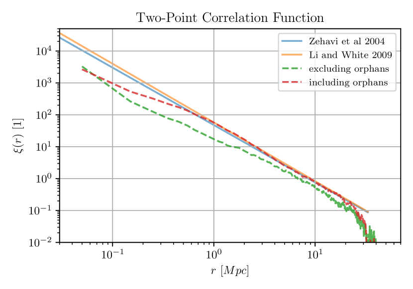
Figure 12: The predicted stellar mass 2-point correlation function (2PCF) $\xi(r)$ of our SHAM model, including and excluding orphan galaxies, compared to the power law fits of the observed 2PCF in Li & White (2009) and Zehavi et al. (2004).

The stellar mass two-point correlation function (2PCF) $\xi(r)$ is computed via inverse Fourier transform of the power spectrum $P(k)$ (e.g. Mo et al., 2011), which itself can be obtained from the Fourier transform of the stellar mass density contrast field $\delta(\mathbf{r})$:

$$\delta_{\mathbf{k}}=\frac{1}{V}\int e^{i\mathbf{kr}}\delta(\mathbf{r})\mathrm{d}^{3}\mathbf{r}$$ (10)

with

$$\delta(\mathbf{r})=\frac{\rho(\mathbf{r})}{\langle\rho(\mathbf{r})\rangle}-1$$ (11)

Where $\rho(\mathbf{r})$ is the galaxy stellar mass density field and $\langle\rho(\mathbf{r})\rangle$ is the corresponding mean density, $V=L^{3}$ is the volume of our large box on which the density field is assumed periodic, and $\mathbf{k}=\frac{2\pi}{L}(i_{x},i_{y},i_{z})$, where $i_{x},i_{y},i_{z}$ are integers. The Fourier transform is performed using the FFTW library (Frigo & Johnson, 2005). The power spectrum $P(k)$ and the 2PCF $\xi(r)$ are given by

$$P(k) =V\langle|\delta_{\mathbf{k}}|^{2}\rangle$$ (12)

$$\xi(r) =\frac{1}{(2\pi)^{3}}\int e^{-i\mathbf{kr}}P(k)\mathrm{d}^{3}\mathbf{k}$$ (13)

The simulation box is divided in a uniform grid of $1024^{3}$ cells and the stellar mass is deposited on the grid using a cloud-in-cell interpolation scheme. The cloud-in-cell scheme consists of assigning each galaxy a cubic volume (“cloud”) the size of a grid cell centered on the galaxy’s position. The galaxy stellar mass is assumed to be uniformly distributed within the cloud, and is deposited on the uniform grid cells according to the volume fraction of the cloud that resides within each cell.

We only include galaxies with masses above $10^{9}M_{\sun}$. Using our adopted SMHM relation, these galaxies are hosted in haloes with mass larger than $\sim 10^{11}M_{\sun}$, or more than 300 particles. This threshold ensures that we only use well resolved clumps for our analysis, as discussed in the previous sections.

The predicted 2PCF $\xi(r)$ is shown in Figure 12, and is compared to the observational results of Li & White (2009) and Zehavi et al. (2004). Note that the observed galaxy catalogue is presented as complete down to $10^{8}M_{\sun}$, one order of magnitude smaller than our simulated catalogue. To highlight the influence of orphan galaxies, we have computed the predicted 2PCF both with and without orphan galaxies. Including orphan galaxies produces a correlation function in much better agreement with observations. Our theoretical 2PCF obtained reproduces the observed power law fit over two orders of magnitude in scale of $r\sim 0.3-25$ Mpc. On the smallest scales, below 0.3 Mpc, our predictions are likely to be affected by our limited mass resolution and the grid resolution which is used for the Fourier Transform ($\sim 0.1$ Mpc per cell). We have verified that using a lower mass threshold for the stellar masses of galaxies makes no visible difference in the resulting correlation function.

The role of the orphan galaxies is particularly important on intermediate scales $\sim 0.2$ Mpc $<\ r\ <2$ Mpc. This behaviour is explained by the fact that orphan galaxies are located within host haloes, thus contributing to the correlations at small distances, the so-called 1-halo term. Our conclusion are in agreement with those of Campbell et al. (2018), who have found that the inclusion of orphan galaxies for mass-based SHAM models improves the clustering statistics of mock galaxy catalogues, particularly so at small scales.

6.2 Radial Profiles of Satellites in Large Clusters

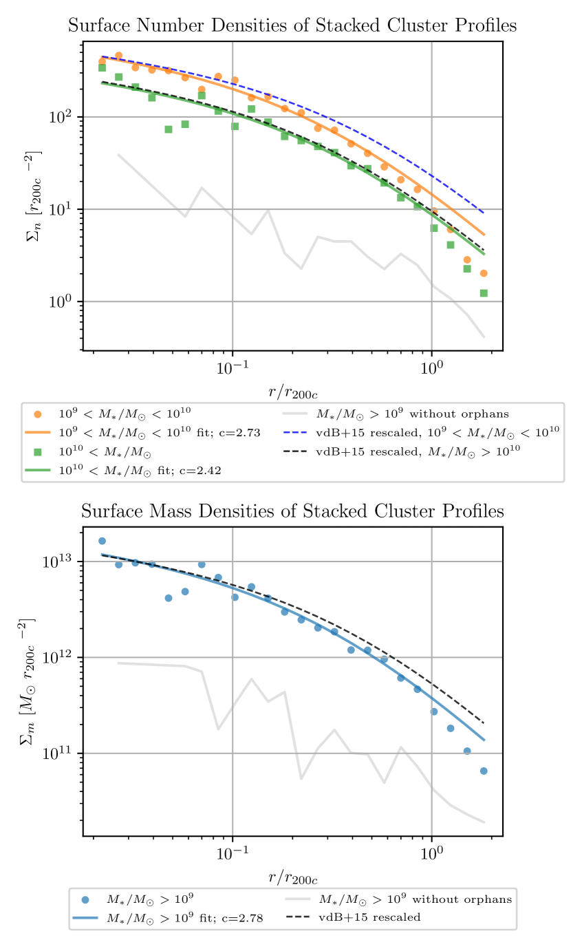
Figure 13: Upper panel: the light grey solid line shows the satellite number density profile averaged over the 10 largest haloes in our simulation including only satellite galaxies with a detected parent clump with masses above $10^{9}M_{\sun}$. Satellites are then grouped in two mass bins indicated in the legend. The colored symbols show the average number density profile including also orphan satellite galaxies. The colored solid lines show the corresponding best fit projected NFW profiles, while the dashed lines show the best fit projected NFW profiles of the observed sample in van der Burg et al. (2015). Note that for the latter, we have renormalized the surface density to match the lower median mass of the simulated sample (see text for details). The lower panel shows the stellar mass surface density averaged over our simulated sample. Here again the light grey solid line shows the mass density profile only for satellite galaxies within a detected clump while the blue symbols shows the same quantity also including orphan satellite galaxies. The blue solid line corresponds to our best fit projected NFW profile while the dashed line shows the best fit NFW profiles of the observed sample in van der Burg et al. (2015). Here again this last profile has been renormalized to account for the difference in median mass between the simulated and the observed cluster samples.

In this section, we compute the radial profiles of number and mass densities of satellite galaxies in the 10 largest clusters in our simulation. In order to compare to observations, we will follow as closely as possible the method described in van der Burg et al. (2015), who analyzed 60 massive clusters between 0.04<$z$<0.26 in the Multi-Epoch Nearby Cluster Survey and the Canadian Cluster Comparison Project.

We identified 10 haloes at $z=0$ with the highest mass. The mass is defined here like in van der Burg et al. (2015) as $M_{200c}$, the mass included within radius $R_{200c}$ at which the average enclosed mass density of the halo is 200 times the cosmological critical density $\rho_{c}$. The $M_{200c}$ masses of our 10 selected haloes range between $1.4\times 10^{14}M_{\sun}$ and $4.8\times 10^{14}M_{\sun}$ with a median value of $1.6\times 10^{14}M_{\sun}$. Due to our limited box size, these haloes are on the lower end of the sample observed in van der Burg et al. (2015), who reported masses ranging from $0.8\times 10^{14}M_{\sun}$ and $1.6\times 10^{15}M_{\sun}$ with a median value of $8.6\times 10^{14}M_{\sun}$.

We compute the projected number density profiles and projected mass density profiles as follows: For each halo, we first project the galaxies (excluding the central galaxy) along each coordinate axis obtaining three images. We then compute cylindrical profiles using radial shells equally space in log radius in units of $r_{200c}$. We then average the 30 profiles (three projections for 10 clusters) to obtain the final average radial surface density profile. Each profile is then fitted to a projected NFW profile (Navarro et al., 1996) using a standard least square fitting procedure. We obtain in particular the concentration parameter that we can compare to the observed value.

The resulting profiles are shown in Figure 13, again including and excluding orphan galaxies. Orphan galaxies play here also a crucial role, as the profiles without orphans underestimate the true value by an order of magnitude. Following van der Burg et al. (2015), we adapt the same galaxy stellar mass $M_{*}$ thresholds of $10^{9}M_{\sun}<M_{*}<10^{10}M_{\sun}$ and $M_{*}>10^{10}M_{\sun}$ for the surface number density profile, and a stellar mass threshold of $M_{*}>10^{9}M_{\sun}$ for the surface mass density profile. It is worth stressing that this lower mass threshold correspond exactly to the mass resolution limit of our mock galaxy catalogue.

As already noted above, the median mass of the simulated and observed catalogues widely differ. In order to facilitate a meaningful comparison, we assume that the total stellar mass in satellites roughly scales with $M_{200c}$ in the halo mass range of interest here. We then adopt the following simple scaling relation

$$\Sigma\propto\frac{M_{200c}}{R_{200c}^{2}}\propto M_{200c}^{1/3}$$ (14)

and rescale the observed average profile found by van der Burg et al. (2015) using this scaling relation and the ratio of the two median masses. We plot in Figure 13 the corresponding best fit projected NFW profiles, showing excellent agreement with our simulated results.

Interestingly, the observed surface density profiles have a slightly smaller concentration than the simulated ones. Although we find for the number densities of satellite galaxies above $10^{10}M_{\sun}$ a concentration $c=2.4$, in strikingly good agreement with $c=2.3$ found by van der Burg et al. (2015) for the same mass range, our results differ for the mass range $10^{9}M_{\sun}<M_{*}<10^{10}M_{\sun}$: we find $c=2.7$ while van der Burg et al. (2015) found $c=1.8$. The same mismatch is found using the mass density profile. we find $c=2.8$, while van der Burg et al. (2015) found $c=2.0$.

We believe that this mismatch in the concentration parameter is consistent with the difference we have in the median sample mass. Indeed, the theory predicts a larger concentration for smaller mass haloes, roughly in the amplitude observed here (Zhao et al., 2009). We therefore could in principle improve the agreement between our simulation results and the observations of van der Burg et al. (2015) by also rescaling the radial direction according to the theoretical expectations. We believe this is beyond the scope of this paper to try and fit exactly the data.

In addition, we believe there is much more to the story. van der Burg et al. (2015) found that larger mass satellite galaxies have a significantly larger concentration parameter than the low mass bin ($c=2.3$ compared to $c=1.8$). Moreover, they have also found a strong excess of satellite galaxies compared to the best fit NFW profile in the centre ($r<0.1R_{200c}$). These observations are consistent with the effect of dynamical friction bringing the more massive galaxies faster to the central regions of the cluster. Dynamical friction is expected to be sufficiently efficient for the most massive sub-haloes, with a mass larger than a few percent of that of the host halos (e.g. Binney & Tremaine, 2008; Mo et al., 2011). In our case, this translates into sub-haloes more massive than a few $10^{12}M_{\sun}$ and satellite galaxies more massive than a few $10^{10}M_{\sun}$. Our simulation clearly suffers from numerical overmerging in this mass range (van den Bosch et al., 2018), as highlighted by the importance of including orphan galaxies in our methodology. Moreover, our pure DMO parent simulation cannot follow precisely the many baryonic effects that are needed to predict accurately the individual trajectory of these higher mass satellite galaxies.

With these caveats in mind, we conclude that using our merger tree code and a state-of-the-art SHAM method, we can model reasonably well the cluster satellite galaxy number density and mass density profiles.

7 Conclusion

We presented ACACIA, a new algorithm to identify dark matter halo merger trees, which is designed to work on-the-fly on systems with distributed memory architectures, together with the adaptive mesh refinement code RAMSES with its on-the-fly clump finder PHEW. Clumps of dark matter are tracked across snapshots through a user-defined maximum number of most bound particles of the clump $n_{mb}$. We found that using $n_{mb}\simeq 200$ tracer particles is a safe choice to obtain robust results for our merger tree algorithm, while not being computationally unrealistically expensive. We also recommend adopting a conservative mass threshold of 200 particles per clump to get rid of a few rare spurious dead branches that would need to be pruned from the halo catalogue anyway.

Additionally, we examined the influence of various definitions of substructure properties on the resulting merger trees. Whether we define substructures to contain their respective substructures’ masses or not had negligible effect on the merger trees. However defining particles to be strictly gravitationally bound to their parent substructure (by requiring that particles can’t leave the spatial extent of that substructure) leads to better results, with much less extreme mass growths and extreme mass growth fluctuations of dark matter clumps. We recommend to use this strictly bound definition as the preferred definition for robust merger trees. The resulting merger trees are in agreement with the bottom-up hierarchical structure formation picture for dark matter haloes. The merger trees of massive haloes at $z=0$ have more branches than their lower mass counterparts. Their formation history can often be traced to very high redshifts.

Once a progenitor clump is merged into a descendant, ACACIA keeps track of the progenitor’s most strongly bound particle, called the “orphan particle”. It is possible for a temporarily merged sub-halo to re-emerge from its host halo at a later snapshot because it hasn’t actually dissolved or merged completely, but only because it wasn’t detected by the clump finder as a separate density peak. Such a situation is illustrated in Figure 4. In these cases, orphan particles are used to establish a link between progenitor and descendant clumps across non-adjacent snapshots. By default, ACACIA will track orphans until the end of the simulation, and orphans are only removed after they have indeed established a link between a progenitor and descendant and thus have served their purpose. Nonetheless, the current implementation offers the option to remove orphan particles after a user defined number of snapshots has passed. Keeping track of orphan particles indefinitely might lead to misidentifications of progenitor-descendant pairs and therefore to wrong formation histories. Our analysis shows however that matches between progenitor-descendant pairs over an interval greater than 10 snapshots are quite rare, so we expect this type of misidentifications to be a negligible issue.

Compared to the test results in Avila et al. (2014), our results are comparable to e.g. the MergerTree, TreeMaker and VELOCIraptor tree builders with AHF, Subfind, or Rockstar halo finders as presented in A14, demonstrating that ACACIA performs similarly to other state-of-the-art tools. However, the performance is inferior to the one of the HBTtree algorithm, which together with the HBThalo halo finder follows structure from one timestep to the next and makes use of this information when constructing both halo catalogues and trees. Furthermore we have encountered issues, e.g. main branch lengths of massive haloes being cut short, due to failures in the PHEW halo finder that we used. In those cases, substructure changed their order in the hierarchy, and the subsequent particle unbinding stripped particles from clumps in lower levels in the hierarchy, preventing ACACIA to establish any links between progenitor and descendant clumps. The resolution of these issues with the clump finder will be a high priority in future work, where we plan on modifying the way PHEW creates the hierarchies. For example, we could define the peak hierarchy not based on the peak density, but rather on the peak mass (e.g. similarly to AdapdaHOP, Aubert et al., 2004). Additionally, with the structure information from previous snapshots available now through ACACIA, further improvements can be made by taking this information into account when constructing the sub-halo hierarchies, in a similar spirit as HBThalo does.

Orphan particles also serve a second purpose besides tracing disappearing clumps. If we also want to produce a mock galaxy catalogue on-the-fly using a dark matter only simulation, the orphan particles are also used to track orphan galaxies. Those are galaxies that don’t have an associated dark matter clump any longer because of numerical overmerging. If we interpret orphan particles as orphan galaxies, there could be additional reasons to consider stopping tracking them. For example, the effects of dynamical friction makes them fall towards the central galaxies. Once the orphan galaxies have lost enough energy, they may find themselves in close proximity to the central galaxies, even below the resolution limit. In these cases, it makes little sense to keep track of these orphans as individual galaxies. They should rather be regarded as merged into the central galaxy, and for that reason removed from the list of tracked orphans. Given that the model we employ doesn’t provide us with the galaxy radii, this approach requires some form of galaxy-galaxy merging cross-sections to compute the probability of a collision between galaxies that will result in a galaxy merger. A different approach that other models use is to estimate the time for orphan galaxies to merge into the parent structure. This estimate could be e.g. the dynamical friction time (as is done in Moster et al. (2013)), or the fitting formula for the merger timescale of galaxies in cold dark matter models by Jiang et al. (2008). These physically motivated approaches to remove orphans will be the subject of future work, where we also intend to make use of the tools and methods presented in Poulton et al. (2018) in order to improve our resulting merger trees and mock galaxy catalogues.

Finally, as a proof of concept and using the known formation history of dark matter clumps from the merger trees and a widely adopted stellar-mass-to-halo-mass relation (Behroozi et al., 2013c), we generate a mock galaxy catalogue from a dark matter only simulation. The influence of the merger trees on the quality of the galaxy catalogues is twofold. First, while the stellar-mass-to-halo-mass relation can be directly applied to central galaxies associated to main haloes, using the peak clump mass for sub-haloes is a better approach for satellite galaxies. The reason is that tidal stripping of galaxies inside a dark matter halo sets in much later than for their host sub-halo (Nagai & Kravtsov, 2005). Second, without properly keeping track of all merging events, no orphan galaxies can be traced, nor can their stellar mass be estimated through the stellar-mass-to-halo-mass relation unless it’s known from which halo the orphan galaxy originated from, and what properties this halo had in the past.

To highlight the impact of the merger trees, we compute observables from our mock galaxy catalogue, both including and excluding orphan galaxies. Specifically, we compute the stellar mass two-point correlation functions and radial profiles of projected number densities and projected stellar mass densities in galaxy clusters. When orphan galaxies are included in the analysis, we obtain correlation functions and radial profiles in good agreement with observations, validating the different steps in our overall methodology.

Data Availability

The data underlying this article will be shared on reasonable request to the corresponding author. The RAMSES  code is publicly available and can be downloaded from https://bitbucket.org/rteyssie/ramses/. Instructions on how to use ACACIA and PHEW during a simulation can be found under https://bitbucket.org/rteyssie/ramses/wiki/Content.

Appendix A Tree Statistics Using Avila et al. (2014) Selection Criteria

Table 6: Comparison of simulation and evaluation parameters used in this work and of A14, where the parameters of the latter have been converted using $h=0.704$. $m_{m}$ is the mass threshold for main haloes, $m_{s}$ is the mass threshold for sub-haloes.

	This work	A14
particle mass [$10^{9}M_{\sun}$]	$1.55$	$1.32$
particles used	$256^{3}$	$270^{3}$
box size [Mpc/h]	$62.5$	$62.5$
snapshots until $z=0$	62	62
$m_{m}$ [$10^{12}M_{\sun}$]	$1.35$	$1.12$ - $1.37$
$m_{s}$ [$10^{11}M_{\sun}$]	$4.03$	$4.26$ - $9.72$

Figure 14: Histograms of the length of the main branch. The top plot shows the length of the 1000 most massive haloes at $z=0$, the bottom plot shows the length of the 200 most massive sub-haloes for $n_{mb}=100$ and $1000$ tracer particles per clump.

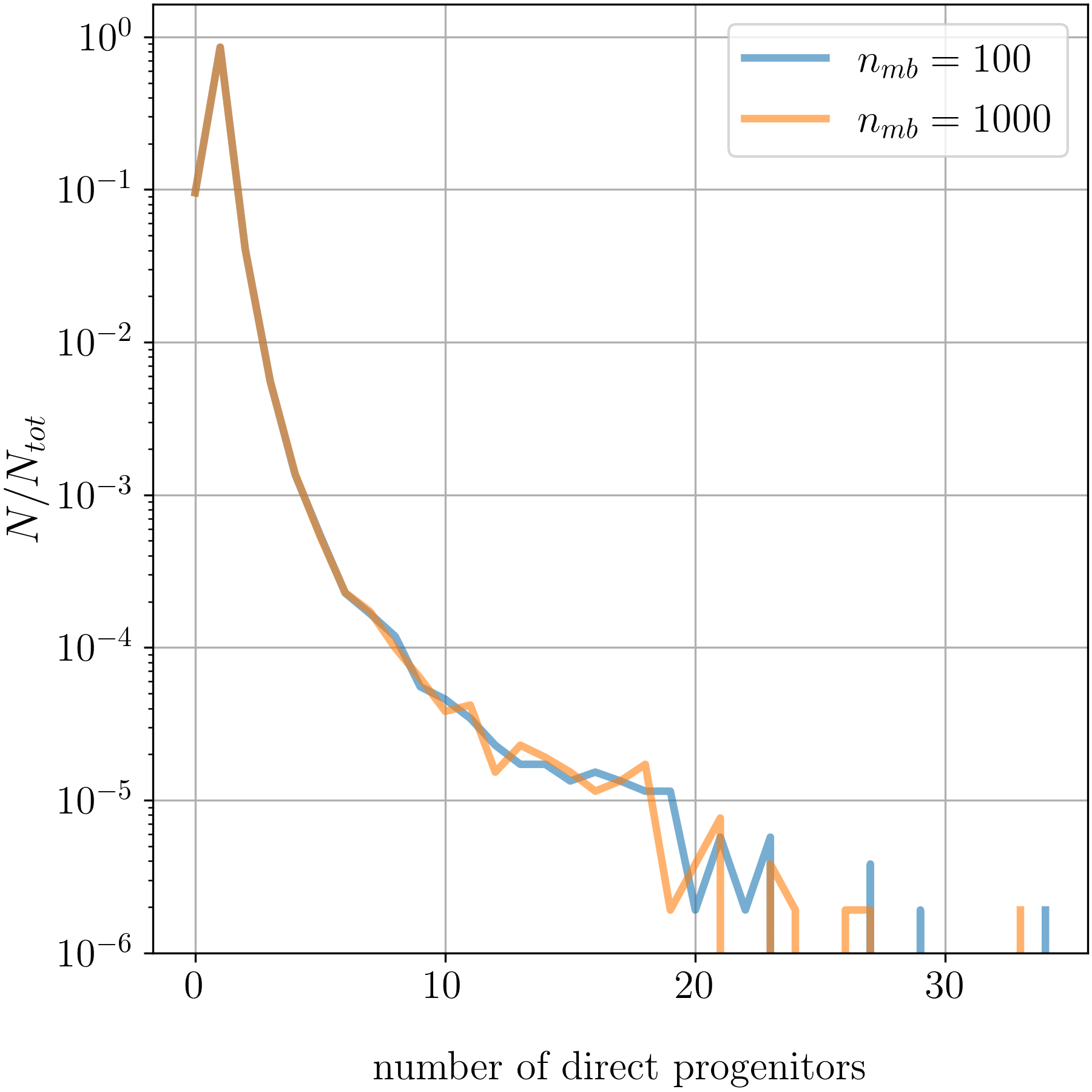
Figure 15: Histogram of the number of direct progenitors for all clumps from $z=0$ to $z=2$ for $n_{mb}=100$ and $1000$ tracer particles per clump. The histogram is normalized by the total number of events found.

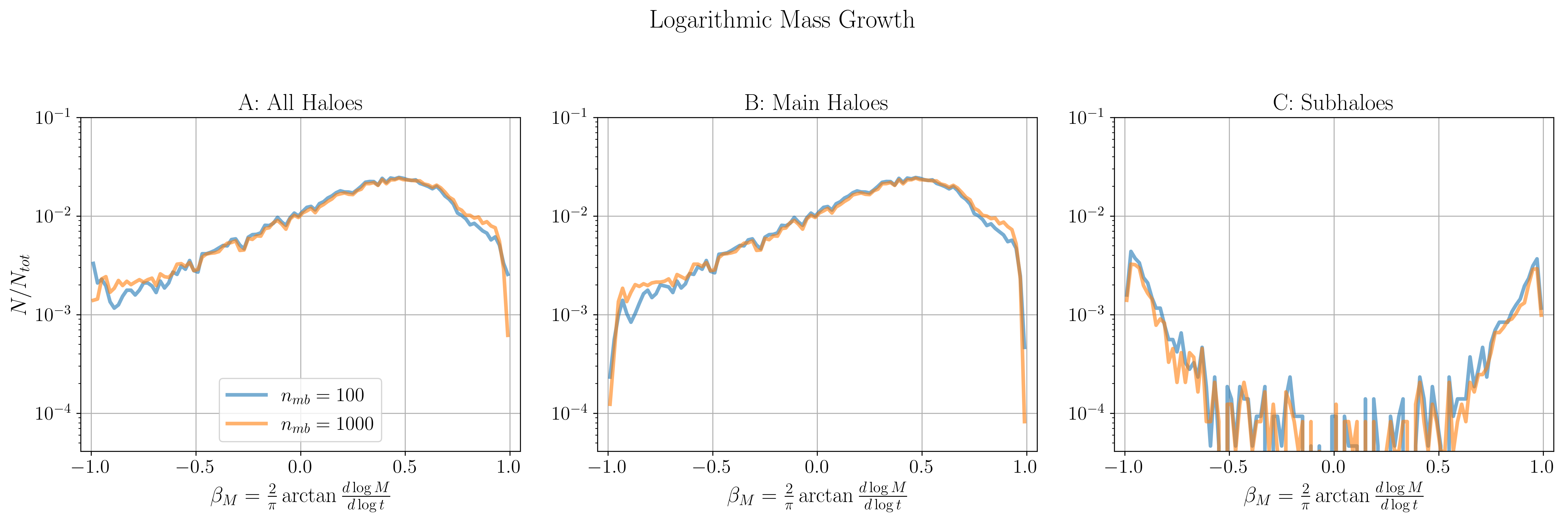
Figure 16: Logarithmic mass growth for haloes and sub-haloes satisfying the mass thresholds. Group $A$ contains clumps that are either haloes or sub-haloes in consecutive snapshots $k$ and $k+1$ with masses $m\geq m_{m}$. Group $B$ contains clumps that are only haloes in two consecutive snapshots with mass above $m_{m}$, group $C$ contains only clumps that were sub-haloes in two consecutive snapshots with mass greater than $m_{s}$. The histogram is normalized by the total number of events found for group $A$.

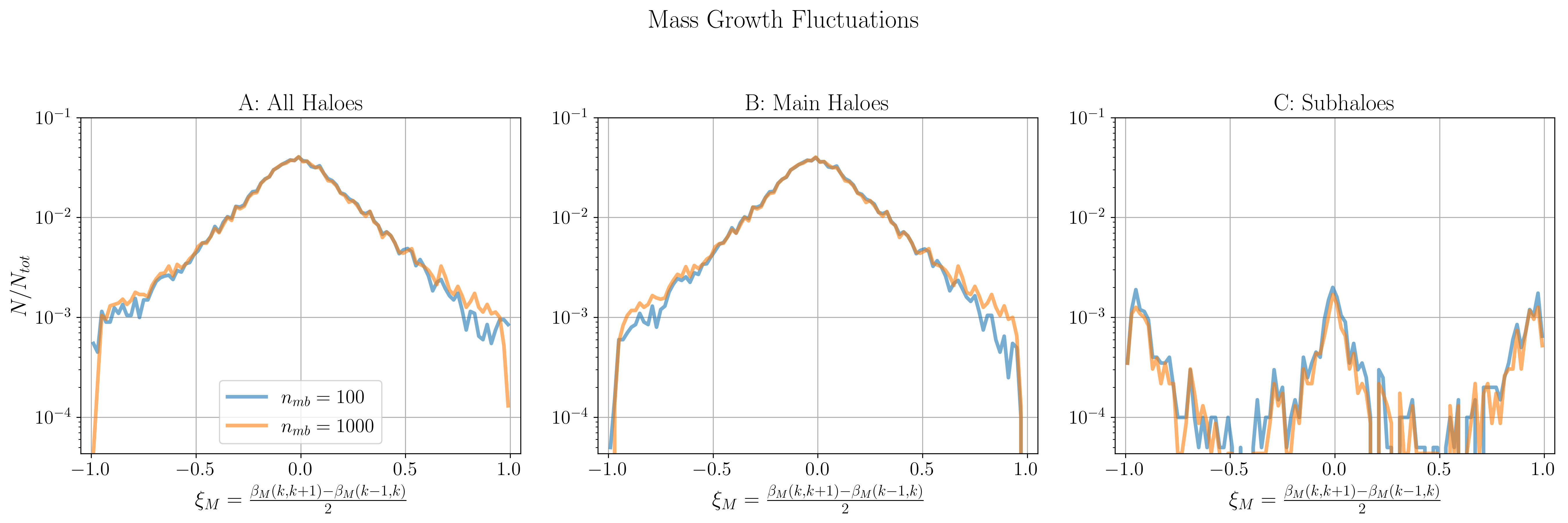
Figure 17: Histogram of mass growth fluctuations for haloes and sub-haloes satisfying the mass thresholds. Group $A$ contains clumps that are either haloes or sub-haloes in three consecutive snapshots with masses $m\geq m_{m}$. Group $B$ contains clumps that are only haloes in three consecutive snapshots with mass above $m_{m}$, group $C$ contains only clumps that were sub-haloes in three consecutive snapshots with mass greater than $m_{s}$. The histogram is normalized by the total number of events found for group $A$.

In this section, the merger tree statistics introduced in Section 5 when following the selection criteria that are used in Avila et al. (2014) (A14 from here on) are presented. Ideally, ACACIA should be tested on the same datasets and halo catalogues used in the Comparison Project to enable a direct comparison to the performance of other merger tree codes. However, since ACACIA was designed to work on the fly, using it as a post-processing utility would defeat its purpose. Furthermore, ACACIA is not necessarily compatible with other definitions of haloes and sub-haloes. But most importantly, we also want to demonstrate that the halo finder PHEW can be used to produce reliable merger trees. So instead, the tests are performed on our own datasets and halo catalogues, which are described in section 5.1. A comparison of the used parameters of our simulations and the ones used in A14 is given in Table 6. In the following, the results for $n_{mb}=100$ and $n_{mb}=1000$ are shown. Like before, when the influence of the number of tracer particles was investigated, the strictly bound parameter and the exclusive mass definition were used.

The difference to the results presented in Section 5 is that the mass thresholds are set such that only the 1000 most massive main haloes and only the 200 most massive sub-haloes at $z=0$ are included. This gives effective mass threshold $m_{m}=1.35\times 10^{12}M_{\sun}$ and $m_{s}=4.0\times 10^{11}M_{\sun}$, which are on one hand comparable to the mass thresholds applied in A14 (Table 6), but already show differences in the resulting halo catalogue. PHEW finds a mass threshold for main haloes that is close to the upper limit found in A13, but a lower mass threshold for sub-haloes. This is consistent with the fact that the strictly bound parameter was used: Unbound particles are passed on to substructure that is higher up in the hierarchy, and the unbinding is repeated until the top level, which are the main haloes, is reached. The more strict unbinding criterion tends to assign more particles to the main haloes and remove them from sub-haloes, which is reflected in the mass thresholds. Indeed, using the loosely bound parameter instead leads to $m_{m}=1.27\times 10^{12}M_{\sun}$ and $m_{s}=1.92\times 10^{12}M_{\sun}$.

The length of the main branches for haloes and sub-haloes individually are shown in Figure 14. Compared to Figure 3 of A14, we note the following similarities and differences:

1. ACACIA finds some main haloes with short (< 10) main branches. In A14, his only happens for the JMerge and TreeMaker tree builders regardless of the halo finder employed, and the MergerTree, SubLink, and VELOCIraptor tree makers for AHF and Subfind halo finders.

2. Like in nearly all cases in A14, the distribution of main branch lengths for main haloes peaks at high numbers and the bulk of the distribution is about 20 snapshots wide. The peak of the main branch length distribution of ACACIA is at 40, while in most cases in A14, it’s around 45 with the exception of the AHF halo finder. This indicates that ACACIA and PHEW result in on average somewhat smaller main branch lengths than other codes. However, we also find the maximal main branch length of 50, while nearly all combinations of halo finders and tree makers in A14 find higher values. Both these differences can be explained by the slightly lower resolution that we used in our simulations, where we found no identifiable clumps before snapshot 11, which corresponds to a maximal main branch length of 51.

3. The main branch lengths for sub-haloes also follow the trends noted above. Additionally, the distribution is flat for main branch lengths smaller than 30, which is not the case for Rockstar and AHF sub-haloes in A14 for nearly all tree builders. Instead, their main branch lengths peak again around unity.

In summary, regarding the main branch lengths of main haloes, PHEW and ACACIA perform comparably to Subfind and Rockstar halo finders and MergerTree, TreeMaker, and VELOCIraptor tree builders. Concerning sub-haloes, the results are most closely to Subfind sub-haloes and the same tree builders as for the main haloes. This is not surprising, because Subfind employs a similar definition of substructure being arbitrarily shaped self-bound structure that is truncated at the isodensity contour that is defined by the density saddle point between the sub-halo and the main halo.

In Figure 15 the number of direct progenitors for all clumps between $z=0$ and $z=2$ are shown. Comparing to Figure 5 of A14, ACACIA gives very comparable results: $\sim 10^{-1}$ haloes have no direct progenitor, almost all have one, and the distribution follows an exponential decay with the maximal number of direct progenitors lying around 20-25, save for a very few outliers. Many tree makers and halo finders in A14 exhibit the same kind of behaviour, particularly so for the AHF, Subfind, and Rockstar all halo finders in Figure 5 of A14.

For the logarithmic mass growth (Figure 16) and the mass growth fluctuations (Figure 17), the statistics are separated into three groups. Group $A$ contains clumps that are either haloes or sub-haloes in consecutive snapshots $k$ and $k+1$ with masses greater than the mass threshold $m_{m}$ in both snapshots. Group $B$ contains clumps that are exclusively main haloes in two consecutive snapshots with mass above $m_{m}$, group $C$ contains only clumps that were sub-haloes in two consecutive snapshots with mass greater than $m_{s}$. We follow clumps of the $z=0$ snapshot along the main branch only.

The logarithmic mass growth resulting from ACACIA follows the general trend that the tree makers in A14 exhibit too. The growth for groups $A$ and $B$ increases steadily and peaks around $\beta_{M}\sim 0.5$, where the peak is $\sim 2\times 10^{-2}$. For $n_{mb}=100$, the extreme mass loss with $\beta_{M}=-1$ increases for group $A$, which is an undesirable property, but is also exhibited by Sublink in A14. For $n_{mb}=1000$, it drops to about $10^{-3}$ ($10^{-4}$ for group $B$), which is comparable behaviour to MergerTree, Sublink, and VELOCIraptor, particularly so in combination with AHF and Subfind halo finders. Group $C$, containing only mass growths of clumps that have been sub-haloes in two consecutive snapshots, shows a distribution peaking around extreme mass growths $\beta_{M}\rightarrow\pm 1$ at $\sim 5\times 10^{-3}$, which can again be seen in A14 for almost all tree makers, albeit not for all halo finders. More noticeably, almost no sub-haloes are found with $-0.5<\beta_{M}<0.5$ with PHEW and ACACIA in Figure 16. This is due to the fact that once a halo is merged into another, it quickly loses its outer mass due to the strict unbinding method used here. However, the distribution that ACACIA finds displays some differences with respect to the results in A14. Firstly, we find almost no mass growth with $-0.5<\beta_{M}<0.5$, similar only to the results of JMerge in A14. This is partially due to the strict selection criteria used for this analysis: We only include clumps that are classified as sub-haloes in two consecutive snapshots and satisfy the mass threshold $m_{s}$ in both snapshots as well. In particular, this excludes all non-adjacent “jumper” links that we find, since we don’t modify the halo catalogue like e.g. ConsistentTrees. Furthermore, we employ the strictly bound unbinding criterium, which strips more particles from sub-haloes and assigns them to main haloes, leaving the halo catalogue with fewer sub-haloes that satisfy the mass threshold. When we instead use the loosely bound criterium, we find that the distribution is on average around $3\times 10^{-4}$ for $-0.5<\beta_{M}<0.5$, albeit noisy, which is in good agreement with most halo finders and tree builders in A14. Secondly, the distribution ACACIA finds looks remarkably symmetric w.r.t. $\beta_{M}=0$. While e.g. MergerTree and TreeMaker trees with AHF, Subfind, and Rockstar haloes find peaks close to $\beta\pm 1$ of similar height, they are also always have distributions skewed towards mass losses $\beta_{M}<0$ and the peaks at $\beta_{M}=-1$ higher than the one at $\beta_{M}=1$.

We found that the reason why our distribution looks so symmetrical is due to the particle unbinding method and the way sub-halo hierarchies are established in PHEW, similarly to what we have found to be a reason for the short main branch lengths in Section 5.2. The hierarchy is determined by the density of the density peak of each clump: A clump with a lower peak density will be considered lower in the hierarchy of substructure. So in situations where two adjacent sub-haloes have similarly high density peaks, their order in the hierarchy might change in between two snapshots due to small changes. The unbinding algorithm then strips the particles from the sub-haloes that have the lowest level in the hierarchy and passes it on to the next level, amplifying the mass loss which these sub-haloes experience. If in the next snapshot the order in the hierarchy for these two clumps are inverted, the clump which experienced a mass loss previously will now experience a strong mass growth and vice versa. In Figure 16 such an oscillation over two snapshots will simultaneously add a strong mass growth and a strong mass loss twice in place of a net smoother mass loss, leading to the symmetry of the distribution. We verified that about 10$\%$ of strong mass growth events with $\beta_{M}>0.75$ are also accompanied by the respective sub-haloes increasing their level in the hierarchy. Similarly, about 10$\%$ of strong mass loss events with $\beta_{M}<-0.75$ are accompanied by the respective sub-haloes decreasing their level in the hierarchy.

The mass growth fluctuations (Figure 17) of ACACIA share the general trend with the ones from Figure 8 in A14, in that they peak around $\xi_{M}=0$ and decrease outwards towards $\xi_{M}=\pm 1$. In A14, in all cases groups $A$ and $B$ peak just below $10^{-1}$, while our results peak around $4\times 10^{-2}$. However, similarly to the results of e.g. Sublink, TreeMaker, and VELOCIraptor with the AHF or Subfind halo finders, the distribution around $\xi_{M}\sim\pm 0.5$ drops to $\sim 5\times 10^{-3}$, and then continues dropping below $10^{-4}-10^{-3}$ at $\xi_{M}\sim\pm 1$. Group $B$ shows a steeper drop around the extreme values $\xi_{M}\sim\pm 1$ compared to group $A$, dropping below $10^{-4}$ at these values, similarly to the behaviour of many tree makers and halo finders in A14. The sub-halo group $C$ of this work shows three main peaks, around $-1$, $0$, and $1$. These peaks also appear in the A14 results. However, the peaks at the extreme values in A14 are lower than the ones of this work, while the peaks around $0$ is higher. The reason why these peaks are so pronounced in our results is the same as for why the mass growths in Figure 16 is remarkably symmetric compared to others: it’s sub-haloes and their respective sub-sub-haloes switching their order in the substructure hierarchy repeatedly and the particle unbinding algorithm stripping particles from the lower level substructure and assigning it to the higher level substructure. The missing values around $\xi_{M}\sim\pm 0.5$ that were also seen in the mass growth in Figure 16 remain unsurprisingly, and are mitigated if the loosely bound unbinding criterion is applied instead. Similar distributions are obtained by e.g. the AHF and Rockstar halo finders in combination with the MergerTree, JMerge, Sublink, and TreeMaker tree builders.

In summary, we find that ACACIA and PHEW produce merger tree statistics which are similar to what multiple other state-of-the-art codes find as well. The results coincide most commonly with those of the AHF, Rockstar, and Subfind halo finders in combination with the MergerTree, TreeMaker, Sublink, and VELOCIraptor tree builders. One notable difference in our result however is that we recover more extreme mass growths and losses as well as fluctuations for sub-haloes due to the way the sub-halo hierarchy is established by PHEW, specifically in cases where a sub-halo and its subsub-halo switch their order in the hierarchy between snapshots.

References

- Aubert et al. (2004) Aubert D., Pichon C., Colombi S., 2004, Monthly Notices of the Royal Astronomical Society, 352, 376
- Avila et al. (2014) Avila S., et al., 2014, MNRAS, 441, 3488
- Behroozi et al. (2013a) Behroozi P. S., Wechsler R. H., Wu H.-Y., 2013a, The Astrophysical Journal, 762, 109
- Behroozi et al. (2013b) Behroozi P. S., Wechsler R. H., Wu H.-Y., Busha M. T., Klypin A. A., Primack J. R., 2013b, ApJ, 763, 18
- Behroozi et al. (2013c) Behroozi P. S., Wechsler R. H., Conroy C., 2013c, ApJ, 770, 57
- Benson et al. (2000) Benson A. J., Cole S., Frenk C. S., Baugh C. M., Lacey C. G., 2000, Monthly Notices of the Royal Astronomical Society, 311, 793
- Berlind & Weinberg (2002) Berlind A. A., Weinberg D. H., 2002, ApJ, 575, 587
- Binney & Tremaine (2008) Binney J., Tremaine S., 2008, Galactic Dynamics: Second Edition
- Bleuler et al. (2015) Bleuler A., Teyssier R., Carassou S., Martizzi D., 2015, Computational Astrophysics and Cosmology, 2, 1
- Bower et al. (2006) Bower R. G., Benson A. J., Malbon R., Helly J. C., Frenk C. S., Baugh C. M., Cole S., Lacey C. G., 2006, MNRAS, 370, 645
- Campbell et al. (2018) Campbell D., van den Bosch F. C., Padmanabhan N., Mao Y.-Y., Zentner A. R., Lange J. U., Jiang F., Villarreal A., 2018, MNRAS, 477, 359
- Chaves-Montero et al. (2016) Chaves-Montero J., Angulo R. E., Schaye J., Schaller M., Crain R. A., Furlong M., Theuns T., 2016, Monthly Notices of the Royal Astronomical Society, 460, 3100
- Conroy et al. (2006) Conroy C., Wechsler R. H., Kravtsov A. V., 2006, The Astrophysical Journal, 647, 201
- Croton et al. (2006) Croton D. J., et al., 2006, Monthly Notices of the Royal Astronomical Society, 365, 11
- Davis et al. (1985) Davis M., Efstathiou G., Frenk C. S., White S. D. M., 1985, ApJ, 292, 371
- Dubois et al. (2014) Dubois Y., et al., 2014, Monthly Notices of the Royal Astronomical Society, 444, 1453
- Elahi et al. (2019) Elahi P. J., Poulton R. J. J., Tobar R. J., Canas R., Lagos C. d. P., Power C., Robotham A. S. G., 2019, Publications of the Astronomical Society of Australia, 36, e028
- Frigo & Johnson (2005) Frigo M., Johnson S. G., 2005, Proceedings of the IEEE, 93, 216
- Guo et al. (2010) Guo Q., White S., Li C., Boylan-Kolchin M., 2010, Monthly Notices of the Royal Astronomical Society, 404, 1111
- Hahn & Abel (2011) Hahn O., Abel T., 2011, MNRAS, 415, 2101
- Harris et al. (2020) Harris C. R., et al., 2020, Nature, 585, 357
- Hunter (2007) Hunter J. D., 2007, Computing in Science Engineering, 9, 90
- Jiang et al. (2008) Jiang C. Y., Jing Y. P., Faltenbacher A., Lin W. P., Li C., 2008, ApJ, 675, 1095
- Jiang et al. (2014) Jiang L., Helly J. C., Cole S., Frenk C. S., 2014, MNRAS, 440, 2115
- Jung et al. (2014) Jung I., Lee J., Yi S. K., 2014, ApJ, 794, 74
- Kang et al. (2005) Kang X., Jing Y. P., Mo H. J., Boerner G., 2005, Astrophys. J., 631, 21
- Kauffmann et al. (1993) Kauffmann G., White S. D. M., Guiderdoni B., 1993, MNRAS, 264, 201
- Khandai et al. (2015) Khandai N., Di Matteo T., Croft R., Wilkins S., Feng Y., Tucker E., DeGraf C., Liu M.-S., 2015, Mon Not R Astron Soc, 450, 1349
- Knebe et al. (2010) Knebe A., Libeskind N. I., Knollmann S. R., Yepes G., Gottlöber S., Hoffman Y., 2010, Mon. Not. R. Astron. Soc.
- Knebe et al. (2011) Knebe A., et al., 2011, MNRAS, 415, 2293
- Knollmann & Knebe (2009) Knollmann S. R., Knebe A., 2009, ApJ, 182, 608
- Komatsu et al. (2011) Komatsu E., et al., 2011, The Astrophysical Journal Supplement Series, 192, 18
- Lacey & Cole (1993) Lacey C., Cole S., 1993, Monthly Notices of the Royal Astronomical Society, 262, 627
- Lee et al. (2014) Lee J., et al., 2014, Mon. Not. R. Astron. Soc., 445, 4197
- Li & White (2009) Li C., White S. D. M., 2009, MNRAS, 398, 2177
- Mo et al. (2011) Mo H., Van den Bosch F., White S., 2011, Galaxy formation and evolution. Cambridge University Press
- Moster et al. (2010) Moster B. P., Somerville R. S., Maulbetsch C., van den Bosch F. C., Macciò A. V., Naab T., Oser L., 2010, ApJ, 710, 903
- Moster et al. (2013) Moster B. P., Naab T., White S. D. M., 2013, MNRAS, 428, 3121
- Nagai & Kravtsov (2005) Nagai D., Kravtsov A. V., 2005, ApJ, 618, 557
- Navarro et al. (1996) Navarro J. F., Frenk C. S., White S. D. M., 1996, The Astrophysical Journal, 462, 563
- Nuza et al. (2013) Nuza S. E., et al., 2013, Monthly Notices of the Royal Astronomical Society, 432, 743
- Onions et al. (2012) Onions J., et al., 2012, Monthly Notices of the Royal Astronomical Society, 423, 1200
- Peacock & Smith (2000) Peacock J. A., Smith R. E., 2000, Monthly Notices of the Royal Astronomical Society, 318, 1144
- Perret (2016) Perret V., 2016, DICE: Disk Initial Conditions Environment, Astrophysics Source Code Library (ascl:1607.002)
- Planck Collaboration et al. (2016) Planck Collaboration et al., 2016, A&A, 594, A13
- Potter et al. (2017) Potter D., Stadel J., Teyssier R., 2017, Computational Astrophysics and Cosmology, 4, 2
- Poulton et al. (2018) Poulton R. J. J., Robotham A. S. G., Power C., Elahi P. J., 2018, Publications of the Astronomical Society of Australia, 35, e042
- Press & Schechter (1974) Press W. H., Schechter P., 1974, ApJ, 187, 425
- Reddick et al. (2013) Reddick R. M., Wechsler R. H., Tinker J. L., Behroozi P. S., 2013, The Astrophysical Journal, 771, 30
- Rodriguez-Gomez et al. (2015) Rodriguez-Gomez V., et al., 2015, Mon. Not. R. Astron. Soc., 449, 49
- Roukema & Yoshii (1993) Roukema B. F., Yoshii Y., 1993, The Astrophysical Journal Letters, 418, L1
- Roukema et al. (1993) Roukema B. F., Quinn P. J., Peterson B. A., 1993, in Observational Cosmology. p. 51
- Schaye et al. (2015) Schaye J., et al., 2015, Monthly Notices of the Royal Astronomical Society, 446, 521
- Scoccimarro et al. (2001) Scoccimarro R., Sheth R. K., Hui L., Jain B., 2001, The Astrophysical Journal, 546, 20
- Seljak (2000) Seljak U., 2000, MNRAS, 318, 203
- Shankar et al. (2006) Shankar F., Lapi A., Salucci P., De Zotti G., Danese L., 2006, The Astrophysical Journal, 643, 14
- Somerville & Primack (1999) Somerville R. S., Primack J. R., 1999, MNRAS, 310, 1087
- Springel et al. (2001) Springel V., White S. D. M., Tormen G., Kauffmann G., 2001, MNRAS, 328, 726
- Springel et al. (2005a) Springel V., et al., 2005a, Nature, 435, 629
- Springel et al. (2005b) Springel V., et al., 2005b, Nature, 435, 629
- Springel et al. (2021) Springel V., Pakmor R., Zier O., Reinecke M., 2021, Monthly Notices of the Royal Astronomical Society, 506, 2871
- Srisawat et al. (2013) Srisawat C., et al., 2013, MNRAS, 436, 150
- Stadel (2001) Stadel J. G., 2001, PhD thesis, University of Washington
- Teyssier, R. (2002) Teyssier, R. 2002, A&A, 385, 337
- Trujillo-Gomez et al. (2011) Trujillo-Gomez S., Klypin A., Primack J., Romanowsky A. J., 2011, The Astrophysical Journal, 742, 16
- Tweed et al. (2009) Tweed D., Devriendt J., Blaizot J., Colombi S., Slyz A., 2009, Astronomy and Astrophysics, 506, 647
- Vale & Ostriker (2006) Vale A., Ostriker J. P., 2006, Monthly Notices of the Royal Astronomical Society, 371, 1173
- Virtanen et al. (2020) Virtanen P., et al., 2020, Nature Methods, 17, 261
- Vogelsberger et al. (2014) Vogelsberger M., et al., 2014, Nature, 509, 177
- Wang et al. (2016) Wang Y., et al., 2016, MNRAS, 459, 1554
- Wechsler et al. (2001) Wechsler R. H., Somerville R. S., Bullock J. S., Kolatt T. S., Primack J. R., Blumenthal G. R., Dekel A., 2001, The Astrophysical Journal, 554, 85
- Wetzel & White (2010) Wetzel A. R., White M., 2010, Monthly Notices of the Royal Astronomical Society, 403, 1072
- White & Frenk (1991) White S. D. M., Frenk C. S., 1991, ApJ, 379, 52
- Zehavi et al. (2004) Zehavi I., et al., 2004, ApJ, 608, 16
- Zentner et al. (2014) Zentner A. R., Hearin A. P., van den Bosch F. C., 2014, Monthly Notices of the Royal Astronomical Society, 443, 3044
- Zhao et al. (2009) Zhao D. H., Jing Y. P., Mo H. J., Boerner G., 2009, The Astrophysical Journal, 707, 354
- van den Bosch et al. (2018) van den Bosch F. C., Ogiya G., Hahn O., Burkert A., 2018, Monthly Notices of the Royal Astronomical Society, 474, 3043
- van der Burg et al. (2015) van der Burg R. F. J., Hoekstra H., Muzzin A., Sifón C., Balogh M. L., McGee S. L., 2015, Astronomy & Astrophysics, 577, A19