Circular statistics-based low complexity DOA
estimation for hearing aid application

Abstract

The proposed Circular statistics-based Inter-Microphone Phase difference estimation Localizer (CIMPL) method is tailored toward binaural hearing aid systems with microphone arrays in each unit. The method utilizes the circular statistics (circular mean and circular variance) of inter-microphone phase difference (IPD) across different microphone pairs. These IPD s are firstly mapped to time delays through a variance-weighted linear fit, then mapped to azimuth direction-of-arrival (DoA) and lastly information of different microphone pairs is combined. The variance is carried through the different transformations and acts as a reliability index of the estimated angle. Both the resulting angle and variance are fed into a wrapped Kalman filter, which provides a smoothed estimate of the DoA. The proposed method improves the accuracy of the tracked angle of a single moving source compared with the benchmark method provided by the LOCATA challenge, and it runs approximately 75 times faster.

Index Terms—  Direction-of-arrival estimation, inter-microphone phase estimation, time difference of arrival, circular statistics, hearing aids.

1 Introduction

Microphone array processing is of interest for hands-free communication, hearing aids, robotics and immersive audio communication systems. It is used in a wide range of applications including noise reduction [1, 2], informed spatial filters for source separation [3, 2], source localization [4] and robust beamforming [5, 6]. The achievable performance in these applications is heavily governed by the accurate information about the direction-of-arrival (DoA) of the target source(s).

Conventional methods for DoA estimation can be grouped into two classes: i) subspace methods relying on e.g. steered-response power phase transform (SRP-PHAT) [7], MUSIC [8] and ESPRIT [9], and ii) cross-power spectrum phase (CSP) based methods [10, 11]. While the methods in the two groups are different in terms of their DoA estimation accuracy and the computational efficiency, among them, CSP is popular due to simplicity and reliability. Of particular importance is the so-called generalized cross correlation (GCC) method using the phase transform (PHAT) normalization [10] for its robustness in DoA estimation for acoustic source localization [11]. More recently, circular statistics has shown a great potential in multi-channel source tracking for both subspace-based [12] and CSP-based [13] methods.

In this paper, we propose CSP-based DoA estimator which relies on circular statistics throughout all estimation stages (Figure 1). Our proposed method, CIMPL, is particularly targeted for application in hearing aids. Specifically, we consider a binaural hearing aid setup consisting of two microphones per hearing aid with a binaural radio connection between each hearing aid. For DoA estimation in such a hearing aid setup, two major challenges are i) the restricted positioning of microphones with a small microphone inter-spacing on each hearing aid and ii) strict computational limitations. We demonstrate the performance of the proposed method with hearing aid recordings in the presence of a single static source (task 1), a single moving source (task 3) and a single moving source with a moving listener (task 5) as defined in the LOCATA challenge [14].

2 DOA estimation

The CIMPL method is based on three major components: i) time difference of arrival (TDoA) estimation, ii) monaural and binaural integration, iii) and source tracking. Figure 1 provides an overview of the CIMPL method. The different stages are explained in the following.

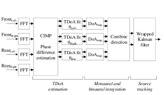
Figure 1: System diagram for the proposed method composed of three stages: i) TDoA estimation relying on CIMP and TDoA fit to left, right and binaural IPD s, ii) data association by integrating the monaural (left and right) and binaural TDoA s, and iii) source tracker using wrapped Kalman filter.

2.1 Time difference of arrival estimation

The initial step in CIMPL is to estimate the TDoA for each microphone set. The TDoA estimation is divided in two stages operating in the frequency domain. The first stage is a phase difference estimation and the second stage consists of a weighted linear fit to estimate the TDoA.

2.1.1 Circular statistics-based inter-microphone phase difference estimation (CIMP)

The instantaneous IPD at frame $l$ and frequency bin $k$, denoted by $\theta_{ab}(k,l)$, defined between two microphones $a$ and $b$ is given by the instantaneous normalized cross-spectrum

$$e^{j\theta_{ab}(k,l)}=\frac{X_{a}(k,l)X_{b}^{*}(k,l)}{\left|X_{a}(k,l)X_{b}(k,l)\right|},$$ (1)

where $X_{a}$ and $X_{b}$ are the short-time Fourier transforms of the input signals at the two microphones and $j=\sqrt{-1}$. We assume that $\theta_{ab}(k,l)$ is a particular realization of a circular random variable $\Theta$. Therefore, the statistical properties of the IPD s are governed by circular statistics and the mean is given by [15, 16]

$$\mathop{\mathbb{E}}\limits_{l}\{e^{j\theta_{ab}(k,l)}\}=R_{ab}(k,l)e^{j\hat{\theta}_{ab}(k,l)},$$ (2)

where $\mathbb{E}$ is a short-time expectation operator (moving average), $\hat{\theta}_{ab}\in[-\pi,\pi[$ is the mean IPD and $R_{ab}\in[0,1]$ is the mean resultant length.

The mean resultant length carries information about the directional statistics of the impinging signals at the hearing aid, specifically about the spread of the IPD. For uniformly distributed $\Theta$, which corresponds to the signal at the two microphones being completely uncorrelated, the associated mean resultant length goes to 0. At the other extreme $\Theta$ is distributed as a Dirac delta function $\Theta\sim\mathcal{W}\left\{\delta(\theta_{ab}-\theta_{0})\right\}$ corresponding to an ideal anechoic source for a specific frequency $f$ at $\theta_{0}=2\pi fd/c\cos{\varphi}$, where $\mathcal{W}\left\{\cdot\right\}$ denotes the transformation that maps a probability density function to its wrapped counterpart [15], $d$ is the inter-microphone spacing, $c$ is the speed of sound, and ${\varphi}$ is the angle of arrival relative to the rotation axis of the microphone pair. In this case, the mean resultant length converges to one.

A particular detrimental type of interference, both for speech intelligibility and for common DoA algorithms, is late reverberation typically modeled as diffuse noise. Diffuse noise is characterized by being a sound field with completely random incident sound waves [17]. This corresponds to the IPD having a uniform probability density $\Theta\sim\mathcal{W}\left\{\mathcal{U}(-\pi f/f_{u},\pi f/f_{u})\right\}$, where $f_{u}=c/(2d)$ is the upper frequency limit where phase ambiguities, due to the $2\pi$-periodicity of the IPD, are avoided. For diffuse noise scenarios, the mean resultant length for low frequencies ($f<<f_{u}$) approaches one. It gets close to zero as the frequency approaches the phase ambiguity limit. Thus, at low frequencies, both diffuse noise and localized sources have similar mean resultant length and it becomes difficult to statistically distinguish the two sound fields from each other.

To resolve the aforementioned limitation, we propose transforming the IPD such that the probability density for diffuse noise is mapped to a uniform distribution $\Theta\sim\mathcal{U}[-\pi,\pi[$ for all frequencies up to $f_{u}$ while preserving the mean resultant length of localized sources. Under free- and far-field conditions and assuming that the inter-microphone spacing is known, the mapped mean resultant length $\tilde{R}_{ab}(k,l)$, which is the mean resultant length of the transformed IPD, takes the form

$$\tilde{R}_{ab}(k,l)=\left|\mathop{\mathbb{E}}\limits_{l}\left\{e^{j\theta_{ab}(k,l)k_{u}/k}\right\}\right|,$$ (3)

where $k_{u}=2Kf_{u}/f_{s}$ with $f_{s}$ being the sampling frequency and $K$ the number of frequency bins up to the Nyquist limit.

The mapped mean resultant length for diffuse noise approaches zero for all $k<k_{u}$ while for anechoic sources it approaches one as intended.

Commonly used methods for estimating diffuse noise (e.g., [18, 19]) are only applicable for $k>k_{u}$. Unlike those methods, the mapped mean resultant length works best for $k<k_{u}$ and is particularly suitable for arrays with very short microphone spacing such as hearing aids. Particularly, by employing the proposed mapped mean resultant length instead of the mean resultant length, correct weighting is applied in time-frequency which takes into account the diffuse noise for low frequency TDoA estimation for small microphone arrays like hearing aid.

Due to the acoustical nature of hearing aid arrays, only frequencies up to $k_{u}$ are considered. At higher frequencies, both for the small spacing between the two microphones on one hearing aid (i.e., monaural case) and across the ears (i.e., binaural case), the assumptions of free- and far-field break down.

2.1.2 Estimating time difference in the frequency domain

Given the mean IPD and the mapped mean resultant lengths calculated so far, the TDoA corresponding to the direct path from a given source needs to be estimated. In free- and far-field conditions the TDoA of a single stationary broadband source corresponds to a constant group delay across frequency, which reduces the problem of estimating the TDoA to fitting a straight line $\theta(f)=2\pi f\tau$. This is effectively done in GCC method by using the inverse Fourier transform and finding the TDoA as the time lag that maximizes the GCC.

Because the IPD s are circular variables, the estimation of TDoA requires solving a circular-linear fit [15]. For a probabilistic interpretation of the regression problem using wrapped IPDs, we refer to [13]. However, since we are only considering frequencies below $f_{u}$, hereby avoiding phase ambiguity, an ordinary linear fit can be used as an approximation. In a commonly used least mean square fit, it is assumed that all data is pulled from a common distribution. However, for each mean IPD, a mapped mean resultant length is estimated, corresponding to a reliability measure of the mean IPD. Due to the aforementioned small inter-microphone spacing in the hearing aid setup, we employ the mapped mean resultant length in (3) instead of the mean resultant length.

Assuming for simplicity that the IPD follows a wrapped normal distribution, the variance ($\sigma_{ab}^{2}$) is given by [15],

$$\sigma_{ab}^{2}(k,l)=-2\log(\tilde{R}_{ab}(k,l)).$$ (4)

For small variances a wrapped normal distribution is well approximated by a normal distribution. However, for small sample sizes, the low mean resultant length values are overestimated, corresponding to an underestimation of the variance, which leads to over emphasizing uncertain data points in the fit. As one way to circumvent this problem, we emprically found that using circular dispersion [15], defined as

$$\delta_{ab}(k,l)=\frac{1-\tilde{R}^{4}_{ab}(k,l)}{2\tilde{R}^{2}_{ab}(k,l)}$$ (5)

for a wrapped normal distribution, deemphasizes the uncertain data points. The reason for this is that $\delta_{ab}$ penalizes low $\tilde{R}$ values more than when using (4), while providing practically the same results for higher $\tilde{R}$ values. Considering that each data point has a known variance given by the circular dispersion and approximating the wrapped normal distribution with the normal distribution, the best least mean square fitted $\tau_{ab}$ takes the form

$$\tau_{ab}(l)=\frac{1}{2\pi}\frac{\sum\limits_{k=1}^{K^{\prime}}\frac{\hat{\theta}_{ab}(k,l)f_{k}}{\delta_{ab}(k,l)}}{\sum\limits_{k=1}^{K^{\prime}}\frac{f_{k}^{2}}{\delta_{ab}(k,l)}},$$ (6)

where $k$ is the frequency bin index, $\hat{\theta}_{ab}$ is the estimated mean IPD from (2) and the summation higher limit $K^{\prime}<K$ denotes the number of frequency bins over which the fit is performed. The actual frequency is $f_{k}=f_{s}k/(2K)$. The variance of the estimated TDoA can, by approximating $\delta_{ab}$ as a deterministic variable, be written as

$$\operatorname{var}\left(\tau_{ab}(l)\right)=\frac{1}{4\pi^{2}}\frac{1}{\sum\limits_{k=1}^{K^{\prime}}\frac{f_{k}^{2}}{\delta_{ab}(k,l)}}.$$ (7)

This expression contains a number of simplifications and it should only be considered as an approximation. However, using (7) allows for a computationally simple closed form approximation of the variance of the estimated TDoA, which can be utilized throughout the further stages to associate data based on their variance.

2.2 Monaural and binaural information integration

From the estimated TDoA and its variance, a local DoA can be estimated for each microphone pair along with its variance. In the proposed method only azimuth DoA is considered and the look direction of the hearing aid user is defined as zero. Three microphone pairs are required in CIMPL: the two (left and right) monaural combinations ($M\in\{L,R\}$) and a binaural ($B$) pair. Additional binaural pairs can be included to improve the accuracy. Assuming far and free field and that the monaural arrays point in the look direction, the local DoA s can be estimated from the monaural TDoA s as follows,

$$\phi_{M}={\arccos}\left(\frac{c}{d_{M}}\tau_{M}\right),$$ (8)

where $d_{M}$ is the inter-microphone spacing between the two microphones on one hearing aid (monaural). Note that, even though the calculations take place at each frame $l$ (i.e., $\phi_{M}\equiv\phi_{M}(l)$), here and in the rest of the paper we drop the time index for conciseness. Using the Taylor expansion of (8) around $\phi_{M}=90^{\circ}$, the variance of the estimated monaural DoA s can be approximated from the variance of the TDoA s as

$$\operatorname{var}\left(\phi_{M}\right)\approx\left(\frac{c}{d_{M}}\right)^{2}\operatorname{var}\left(\tau_{M}\right),$$ (9)

where the $\operatorname{var}\left(\tau_{M}\right)$ is estimated using (7).

For the binaural microphone pair, we assume far field and an ellipsoidal head model [20]. From this, the binaural DoA is well approximated by

$$\phi_{B}\approx\left(\frac{c}{d_{B}}\tau_{B}\right),$$ (10)

where $d_{B}$ is the inter-microphone spacing between the two hearing aids on the head and the look direction is perpendicular to the rotation axis of the binaural microphone pair. The variance of the estimated binaural DoA can be written as

$$\operatorname{var}\left(\phi_{B}\right)=\left(\frac{c}{d_{B}}\right)^{2}\operatorname{var}\left(\tau_{B}\right).$$ (11)

The estimated DoA s are circular variables and their estimated variances are transformed to mean resultant lengths using (4), where each DoA is assumed to follow a wrapped normal distribution. We denote $R_{M}$ ($M\in\{L,R\}$) and $R_{B}$ as the monaural and the binaural mean resultant lengths associated with the angle of arrivals, respectively.

The monaural DoA estimates for the left and the right pairs are defined in the interval $[0,\pi]$ due to the rotational symmetry around the line connecting the microphones. Correspondingly, the binaural DoA is defined within $[-\pi/2,\pi/2]$. In order to combine the information from the monaural pairs and the binaural pair, a common support must be established. This is accomplished by mapping all azimuth estimates onto the full circle ($\varphi\in[-\pi,\pi[$). The choice of the monaural mean resultant length depends on which hearing aid is closer to the source. Using the binaural pair, we determine whether a given source is to the left ($\phi_{B}\geq 0$) or the right ($\phi_{B}<0$). Based on this, if the source is located on the left, the left monaural microphone pair is chosen ($\varphi_{M}=\phi_{L}$), and similarly on the right side ($\varphi_{M}=-\phi_{R}$). Due to the head shadow effect, the monaural microphone pair closer to the source yields a more reliable estimate. From the chosen monaural pair it can be determined if a potential source is in front of ($|\varphi_{M}|\leq\pi/2$) or behind ($|\varphi_{M}|>\pi/2$) the hearing aid user. When a source is in the front, then $\varphi_{B}=\phi_{B}$. If the source is determined to be to the right and behind the wearer, then $\varphi_{B}=-\pi-\phi_{B}$, and if it is behind and to the left, then $\varphi_{B}=\pi-\phi_{B}$. The mean resultant lengths are invariant under translations and are converted directly.

We have a monaural and a binaural azimuth estimate of the full-circle DoA with their mean resultant lengths. From this, a statistical test is performed to assess the null hypothesis that the two estimates have a common mean [15]. The modified test statistic that we employ is

$$Y = 2\left(\left(\frac{w_{M}}{\delta_{M}}+\frac{w_{B}}{\delta_{B}}\right)-\sqrt{C^{2}+S^{2}}\right),$$ (12)

where $C$ and $S$ are given by

$$C = \frac{w_{M}}{\delta_{M}}\cos(\varphi_{M})+\frac{w_{B}}{\delta_{B}}\cos(\varphi_{B}),$$ (13)

$$S = \frac{w_{M}}{\delta_{M}}\sin(\varphi_{M})+\frac{w_{B}}{\delta_{B}}\sin(\varphi_{B}).$$

Here, $\delta$ is the circular dispersion known from (5), $w_{M}={\sin}^{2}(\varphi_{M})$ and $w_{B}={\cos}^{2}(\varphi_{B})$ are weighting factors for the monaural and binaural estimates, respectively, and $Y$ is the test statistic to be compared with the upper 100(1-$\alpha$)% point of the $\chi^{2}_{1}$ distribution, with $\alpha$ as the significance level. The weighting factors are used to effectively reduce the reliability of the estimates to compensate for the approximations made in (9) and (11). If the null hypothesis is accepted with $\alpha=0.1$, a common mean direction $\hat{\varphi}$ of the two estimates is calculated as [15]

$$\hat{\varphi} = \angle\{w_{1}R_{M}e^{i\varphi_{M}}+w_{2}R_{B}e^{i\varphi_{B}}\},$$ (14)

with

$$w_{1} = \frac{w_{M}/\left(R_{M}\delta_{M}\right)}{w_{M}/\left(R_{M}\delta_{M}\right)+w_{B}/\left(R_{B}\delta_{B}\right)},$$

$$w_{2} = \frac{w_{B}/\left(R_{B}\delta_{B}\right)}{w_{M}/\left(R_{M}\delta_{M}\right)+w_{B}/\left(R_{B}\delta_{B}\right)}.$$

Similarly, the circular dispersion of the common mean direction is

$$\delta = 2\frac{w_{1}^{2}R_{M}^{2}\delta_{M}+w_{2}^{2}R_{B}^{2}\delta_{B}}{\left(w_{1}R_{M}+w_{2}R_{B}\right)^{2}}.$$ (16)

Subsequently, the mean resultant length of the common mean can be calculated by solving (5) for $R$ using the circular dispersion obtained by (16) yielding

$$R=\frac{1}{\sqrt{\delta+\sqrt{1+\delta^{2}}}}.$$ (17)

If the null hypothesis is rejected, the DoA and its mean resultant length are chosen from the estimate with the lowest circular dispersion, i.e., either the monaural or the binaural.

From the above development, the information provided from the monaural and the binaural TDoA s and their variance are combined to make a unified full-circle DoA $\hat{\varphi}$ estimate in (14) with an accompanying circular dispersion $\delta$ in (16) and the mean resultant length $R$ in (17).

2.3 Source tracking

The azimuth estimation at the output from the previous stage is very noisy, but at the same time it is accompanied by an instantaneous indication of reliability in the form of the mean resultant length $R$ (17) or the circular dispersion (16). We include an angle-only wrapped Kalman filter [21] to obtain a smoother estimate. Differently from the original method described in [21], which assumes a fixed and known variance denoted by $\sigma_{w}^{2}$ for the innovation term, we update this quantity at each frame using the circular dispersion as an approximation, i.e. $\sigma^{2}_{w_{t}}\approx\delta$. By using circular dispersion provided in (17) instead of variance, low $R$ values map onto higher $\sigma^{2}_{w}$ values.

3 Evaluation

The LOCATA challenge development dataset [14] was used to assess the performance of CIMPL. More specifically, the hearing aid recordings in the presence of a single static source (task 1), a single moving source (task 3) and a single moving source with a moving listener (task 5) were considered.

The standard deviation of the process noise in the wrapped Kalman filter was set to 1^∘. Figure 2 illustrates the behavior of the algorithm for a recording of a single moving source. Notice that the raw azimuth estimates, shown in gray on the top panel, were very noisy. In contrast, the tracked angles, shown in red on the top panel, are smoother and more accurate thanks to the use of a wrapped Kalman filter. The input measurement variance to the wrapped Kalman filter was updated at each frame with the dispersion $\delta$, related to the reliability factor of the estimates, shown in red on the bottom panel, shown in Figure 2.

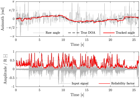
Figure 2: [Top] Azimuth tracking of a single moving source with CIMPL (red) and ground truth (dashed), together with raw angle estimates before the wrapped Kalman filter (gray). [Bottom] Raw audio signal (gray) and the reliability factor (red) used as input to the wrapped Kalman filter.

The mean absolute deviation from the ground truth (with standard deviation shown in parentheses), averaged across all data segments where speech was active, was 5.9^∘ (10.4^∘) for task 1, 8.2^∘ (8.2^∘) for task 3, and 18.7^∘ (23.5^∘) for task 5.

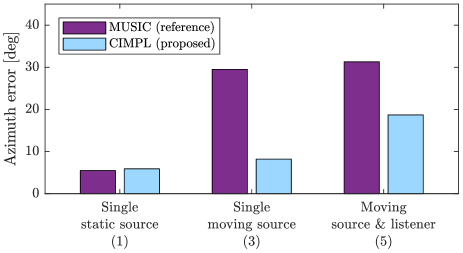
Figure 3: Azimuth accuracy for Tasks 1, 3 and 5 for the hearing aid recordings of the LOCATA challenge development dataset [14].

As shown in Figure 3, the performance of CIMPL in task 1 is comparable to that provided by the tracked MUSIC algorithm provided by LOCATA Challenge [14] as the benchmark, and better in tasks 3 and 5. Moreover, CIMPL runs in 1.3% of the CPU time required by the tracked MUSIC algorithm [14] provided in the LOCATA challenge.

4 Concluding remarks

In this paper we proposed a new DoA estimator targeted for tracking a single source with a binaural hearing aid setup. By estimating the angle via circular statistics, the mean resultant length is obtained which acts as a reliability index. The mean resultant length is then carried throughout all the processing steps and is used at the tracker to improve the accuracy of the tracked angle.

Performance evaluation of the proposed method on the hearing aid recordings provided in the development dataset of the LOCATA challenge [14] revealed an improved accuracy of the tracked angle of a single moving source compared to the benchmark method (tracked MUSIC algorithm) provided by the organizers, while running approximately 75 times faster. The low computational complexity of our algorithm makes it a favorable choice for hearing aid application. The estimated angle may be used at further stages of potential hearing aid processing, such as informed beamforming or scene classification.

References

- [1] A. Schwarz and W. Kellermann, “Coherent-to-Diffuse Power Ratio Estimation for Dereverberation,” IEEE Transactions on Audio, Speech and Language Processing, vol. 23, no. 6, pp. 1006–1018, 2015.
- [2] S. Chakrabarty and E. A. Habets, “A Bayesian approach to informed spatial filtering with robustness against DOA estimation errors,” IEEE Transactions on Audio, Speech and Language Processing, vol. 26, no. 1, pp. 145–160, 2018.
- [3] O. Thiergart, M. Taseska, and E. A. P. Habets, “An Informed Parametric Spatial Filter based on Instantaneous Direction-of-Arrival Estimates,” IEEE Transactions on Audio, Speech and Language Processing, vol. 22, no. 12, pp. 1–15, 2014.
- [4] M. Farmani, M. S. Pedersen, Z.-H. Tan, and J. Jensen, “Informed Sound Source Localization Using Relative Transfer Functions for Hearing Aid Applications,” IEEE/ACM Transactions on Audio, Speech, and Language Processing, vol. 25, no. 3, pp. 611–623, 2017.
- [5] D. P. Jarrett, E. A. Habets, M. R. Thomas, N. D. Gaubitch, and P. A. Naylor, “Dereverberation performance of rigid and open spherical microphone arrays: Theory & simulation,” 2011 Joint Workshop on Hands-free Speech Communication and Microphone Arrays, HSCMA’11, no. April, pp. 145–150, 2011.
- [6] S. Gannot and I. Cohen, “Adaptive beamforming and postfiltering,” in Handbook of Speech Processing, J. Benesty, M. M. Sondhi, and H. Yiteng, Eds. Springer Berlin Heidelberg, 2008, ch. 10, pp. 945–978.
- [7] J. H. Dibiase, “A high-accuracy, low-latency technique for talker localization in reverberant environments using microphone arrays,” Ph.D. dissertation, Brown University, 2000.
- [8] R. O. Schmidt, “Multiple emitter location and signal parameter estimation,” IEEE Transactions on Antennas and Propagation, vol. 34, pp. 276–280, Mar. 1986.
- [9] R. Roy and T. Kailath, “ESPRIT-estimation of signal parameters via rotational invariance techniques,” IEEE Trans. Acoustics, Speech, and Signal Processing, vol. 37, no. 7, pp. 984–995, 1989.
- [10] C. H. Knapp and G. C. Carter, “The generalized correlation method for estimation of time delay,” IEEE Transactions on Acoustics, Speech and Signal Processing, vol. ASSP-24, no. 4, pp. 320–327, 1976.
- [11] M. Omologo and P. Svaizer, “Acoustic source location in noisy and reverberant environment using CSP analysis,” IEEE International Conference on Acoustics, Speech, and Signal Processing (ICASSP), vol. 2, no. October 2014, pp. 921–924 vol. 2, 1996.
- [12] M. Taseska and E. A. Habets, “DOA-informed source extraction in the presence of competing talkers and background noise,” EURASIP Journal on Advances in Signal Processing, vol. 2017, no. 1, 2017.
- [13] J. Traa and P. Smaragdis, “Multichannel source separation and tracking with RANSAC and directional statistics,” IEEE/ACM Transactions on Audio Speech and Language Processing, vol. 22, no. 12, pp. 2233–2243, 2014.
- [14] H. W. Löllmann, C. Evers, A. Schmidt, H. Mellmann, H. Barfuss, P. A. Naylor, and W. Kellermann, “The LOCATA challenge data corpus for acoustic source localization and tracking,” in IEEE Sensor Array and Multichannel Signal Processing Workshop (SAM), Sheffield, UK, July 2018.
- [15] N. I. Fisher, Statistical Analysis of Circular Data. Cambridge Unviersity Press, 1993.
- [16] K. V. Mardia and P. E. Jupp, Directional Statistics. John Wiley & Sons, 2000.
- [17] R. K. Cook, R. V. Waterhouse, R. D. Berendt, S. Edelman, and M. C. Thompson, “Measurement of correlation coefficients in reverberant sound fields,” The Journal of the Acoustical Society of America, vol. 27, no. 6, pp. 1072–1077, 1955.
- [18] J. B. Allen, D. A. Berkley, and J. Blauert, “Multi microphone signal-processing technique to remove room reverberation from speech signals,” The Journal of the Acoustical Society of America, vol. 62, no. 4, pp. 912–915, 1977.
- [19] A. Westermann, J. M. Buchholz, and T. Dau, “Binaural dereverberation based on interaural coherence histograms,” The Journal of the Acoustical Society of America, vol. 133, no. 5, pp. 2767–2777, 2013.
- [20] R. Duda, C. Avendirno, and J. R. Algazi, “An adaptable ellipsoidal head model for the interaural time difference,” in ICASSP, 1999, pp. 965–968.
- [21] J. Traa and P. Smaragdis, “A wrapped Kalman filter for azimuthal speaker tracking,” IEEE Signal Processing Letters, vol. 20, no. 12, pp. 1257–1260, 2013.