Abstract

We present an overview of the recent lattice determination of the QCD coupling $\alpha_{s}$ by the ALPHA Collaboration. The computation is based on the non-perturbative determination of the $\Lambda$-parameter of ${N_{\rm f}}=3$ QCD, and the perturbative matching of the ${N_{\rm f}}=3$ and ${N_{\rm f}}=5$ theories. The final result: $\alpha_{s}(m_{Z})=0.11852(84)$, reaches sub-percent accuracy.

4 1 148 Received: 28 November 2018; Accepted: 13 December 2018; Published: 15 December 2018 yes Precision Determination of $\alpha_{s}$ from Lattice QCD Mattia Dalla Brida ^1,2,* on behalf of the ALPHA Collaboration Mattia Dalla Brida Correspondence: mattia.dallabrida@unimib.it

1 Introduction

The strong coupling $\alpha_{s}$ is a fundamental parameter of QCD and therefore of the Standard Model (SM) of Particle Physics. Its value affects the result of any perturbative calculation involving the strong interactions, and hence virtually all cross section calculations for processes at the Large Hadron Collider. It also impacts considerations on the stability of the electroweak vacuum, grand unification arguments, and searches of new coloured sectors. At present, the PDG world average for the strong coupling has an uncertainly $\delta\alpha_{s}/\alpha_{s}\approx 0.9\%$ Tanabashi et al. (2018). The coupling of QCD is thus by orders of magnitude, the least-precisely determined coupling among those characterizing the (known) fundamental forces of nature. From the point of view of phenomenology, the current uncertainty on $\alpha_{s}$ leads to relevant, i.e., 3–7%, uncertainties in key Higgs processes such as $gg\to H$ and associated $H-t\bar{t}$ cross sections, and $H\to b\bar{b},c\bar{c},gg$ branching fractions. This uncertainty on $\alpha_{s}$ is moreover expected to dominate the parametric uncertainties in determinations of the top-quark mass and electroweak precision observables at future colliders (see e.g., d’Enterria (2018) and references therein). A determination of $\alpha_{s}$ comfortably below the per-cent level is called for in precision tests of the SM.

Currently, $\alpha_{s}$ is determined by the PDG by combining the results from different sub-categories Tanabashi et al. (2018). In short, the results from the different sub-fields are first pre-averaged, in such a way to take into account the spread among the different determinations (cf. Figure 1). The sub-averages are then assumed to be independent and the final result for $\alpha_{s}$ is computed by $\chi^{2}$-averaging these (cf. Ref. Tanabashi et al. (2018)). The essential reason for the pre-averages is to obtain a more realistic estimate of $\alpha_{s}$ from the different sub-fields. Many determinations are in fact affected by systematic uncertainties which are hard to quantify. It is thus likely that in some cases these might have been underestimated to some degree, causing the observed spread. The situation is hence not quite satisfactory in general. For several determinations, the attainable precision on $\alpha_{s}$ is likely limited by intrinsic sources of systematics, which in practice cannot be estimated to the desired level of precision. In order to achieve a precise and accurate determination of the QCD coupling, it is thus mandatory to develop methods where all sources of uncertainty can reliably be kept under control. In this light, one might even object to the way $\alpha_{s}$ is currently determined. In the case of other fundamental parameters, only a small set of accurate procedures, if not a single one, is actually considered for their determination, while the others are intended as tests of the theory. As we shall discuss below, however, in the case of $\alpha_{s}$, finding such an accurate procedure is no simple task.

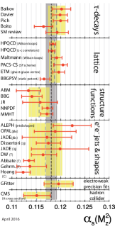
Figure 1: PDG summary of $\alpha_{s}$-determinations from six chosen sub-fields Tanabashi et al. (2018). The yellow (light shaded) bands and dashed lines indicate the pre-average values of each sub-field. The dotted line and grey (dark shaded) band represent the final world average vale of $\alpha_{s}$.

The outline of this contribution is the following. In the next section, we overview how the strong coupling is generally determined in phenomenology, emphasizing in particular the main difficulties one encounters. We then move on to discuss determinations based on lattice QCD methods, which are the focus of this presentation. We first discuss how a naive approach has to face similar shortcomings as most phenomenological determinations, and see how these can be overcome by introducing finite-volume renormalization schemes and step-scaling techniques. The rest of the discussion is dedicated to presenting a specific lattice determination using these methods, recently completed by the ALPHA Collaboration Dalla Brida et al. (2016, 2017); Bruno et al. (2017); Dalla Brida et al. (2018). The remarkable aspect of this result is that it achieves a sub-percent precision determination of $\alpha_{s}$ where the final error is dominated by statistical rather than systematic uncertainties. We finally conclude discussing some future directions on how this result could be further improved.

2 Determinations of $\alpha_{s}$: General Considerations

2.1 Phenomenological Determinations

Any phenomenological determination of $\alpha_{s}$ is essentially based on the following idea (see e.g., Ref. Salam (2019)). One considers an experimental observable $\mathcal{O}(q)$ depending on an overall energy scale $q$; for simplicity, we ignore any dependence on additional kinematic variables. This observable is then compared with its theoretical prediction in terms of a perturbative expansion in $\alpha_{s}(\mu)\equiv\alpha_{\overline{\rm MS}}(\mu)$:

$$\mathcal{O}_{\rm th}(q)=\sum_{n=0}^{N}c_{n}(s)\alpha_{s}^{n}(\mu)+{\rm O}(\alpha_{s}^{N+1})+{\rm O}\Big{(}{\Lambda^{p}\over q^{p}}\Big{)},\quad\mu={q\over s},$$ (1)

where the renormalization scale $\mu$ is set proportional to $q$ through the parameter $s$. The factors $c_{n}$ appearing in this equation are the coefficients of the perturbative series, which depend on the choice of renormalization scheme made for the coupling and on the scale factor $s$. In practice, these are known up to some finite order $N$. Requiring: $\mathcal{O}_{\rm th}(q)=\mathcal{O}(q)$ fixes the value of the coupling $\alpha_{s}(\mu)$ up to some error, which comes from several different sources. First of all, the precision $\delta\mathcal{O}(q)$ to which the observable $\mathcal{O}(q)$ is known experimentally. It is the general situation that, when $q$ becomes large, and hence most sources of uncertainty become small (s. below), the experimental errors in $\mathcal{O}(q)$ also get large. Second, is the effect of missing perturbative orders, i.e., the size of the ${\rm O}(\alpha_{s}^{N+1})$ terms in Equation (1). When the available measurements of $\mathcal{O}(q)$ allow it, this is normally accessed by studying the agreement between extractions of $\alpha_{s}(\mu)$ at different values of $q$, which are compared at some common reference scale through perturbative running. As we shall see in a realistic case (cf. Section 4.1), in order to reliably access this error, it is necessary to vary $q$ over a wide range, reaching up to large values (say O($100\,{\rm GeV}$)). In the situation where $q$ cannot really be varied, the ${\rm O}(\alpha_{s}^{N+1})$ terms are usually estimated by studying the size of the known perturbative terms and their “convergence”. Another strategy is to study the effect of varying $\mu$ rather than $q$, or equivalently the parameter $s$. Due to the asymptotic character of the perturbative expansion, however, estimating the contribution of missing perturbative orders within perturbation theory itself is in principle an impossible task. In practice, this procedure is particularly questionable if $q$ is not really large and hence far from the region of asymptoticity. Another source of uncertainty in the extraction of $\alpha_{s}$ is the size of “non-perturbative contributions”. These are formally represented in Equation (1) by some power corrections to the perturbative expansion of ${\rm O}({\Lambda^{p}/q^{p}})$, where $p>0$ and $\Lambda$ is some characteristic non-perturbative scale of QCD. In fact, our knowledge of the form of non-perturbative effects is rather limited. It is hence always debatable whether any model that tries to capture them is really adequate to the describe the data within a given accuracy. A more systematic way to deal with the problem is again to study the extraction of $\alpha_{s}$ for a wide range of (large) $q$-values, and access whether the use of perturbation theory alone gives consistent results. This in general means accessing whether any observed discrepancy is consistent with the effect of missing higher-order terms in the perturbative expansion. Finally, one should always keep in mind that any experimental observable $\mathcal{O}$ is in principle sensitive to all kinds of physics. The theoretical description of $\mathcal{O}$ given by Equation (1) might thus be missing, e.g., higher-order electroweak corrections, uncertainties associated with other SM parameters, or even effects from yet unknown physics.

In conclusion, a precise phenomenological determination of $\alpha_{s}$ has to face many challenges, and many determinations are limited in their precision by one or more of the above issues. In the following sections, we would like to argue that extracting $\alpha_{s}$ using lattice QCD methods, on the other hand, allows in principle to circumvent many of these limitations.

2.2 Phenomenological Couplings and $\Lambda$-Parameters

For the discussion that will follow, it is useful to introduce the concepts of phenomenological couplings and their $\Lambda$-parameters (see e.g., Ref. Sommer and Wolff (2015) for a more extensive presentation). We can indeed associate to any short-distance observable ${\mathcal{O}}(q)$ a renormalized coupling $\alpha_{\mathcal{O}}(\mu)$ as ($c_{n}\equiv c_{n}(1)$):

$$\alpha_{\mathcal{O}}(\mu)\equiv{\bar{g}^{2}_{\mathcal{O}}(\mu)\over 4\pi}\equiv{{\mathcal{O}}_{\rm th}(\mu)-c_{0}\over c_{1}}\overset{\mu\to\infty}{=}\alpha_{s}(\mu)+{c_{2}\over c_{1}}\alpha_{s}^{2}(\mu)+\ldots\,.$$ (2)

In this language, the extraction of $\alpha_{s}$ through ${\mathcal{O}}_{\rm th}$ is interpreted as the perturbative matching between the couplings $\alpha_{\mathcal{O}}$ and $\alpha_{s}$, where different observables ${\mathcal{O}}$ correspond to different renormalization schemes.

The value of the coupling $\bar{g}_{\mathcal{O}}(\mu)$ at any renormalization scale is in one-to-one correspondence with the $\Lambda$-parameter:

$$\Lambda_{\mathcal{O}}=\mu\times(b_{0}\bar{g}^{2}_{\mathcal{O}}(\mu))^{-b_{1}/(2b_{0}^{2})}e^{-1/(2b_{0}\bar{g}^{2}_{\mathcal{O}}(\mu))}\times\exp\bigg{\{}-\int_{0}^{\bar{g}_{\mathcal{O}}(\mu)}{\rm d}g\bigg{[}{1\over\beta_{\mathcal{O}}(g)}+{1\over b_{0}g^{3}}-{b_{1}\over b_{0}^{2}g}\bigg{]}\bigg{\}}.$$ (3)

In this equation: $\beta_{\mathcal{O}}(g)\equiv[\mu{\rm d}\bar{g}_{\mathcal{O}}(\mu)/{\rm d}\mu]|_{g}$, is the well-known $\beta$-function, describing the dependence of the coupling on the renormalization scale. In perturbation theory, we have:

$$\beta_{\mathcal{O}}(g)\overset{g\to 0}{\to}-b_{0}g^{3}-b_{1}g^{5}-b^{\mathcal{O}}_{2}g^{7}+\ldots,\quad b_{0}=\big{(}11-\hbox{$2\over 3$}{N_{\rm f}}\big{)}(4\pi)^{-2},\quad b_{1}=\big{(}102-\hbox{$38\over 3$}{N_{\rm f}}\big{)}(4\pi)^{-4},$$ (4)

where ${N_{\rm f}}$ is the number of (massless) quark-flavours considered. The coefficients $b_{0},b_{1}$ are universal and shared by all mass-independent renormalization schemes; the scheme dependence only enters through the higher-order coefficients $b_{i}^{\mathcal{O}}$, $i\geq 2$. It is easy to show that this implies a simple scheme dependence for the $\Lambda$-parameters. Specifically, we have that: ${\Lambda_{\rm X}/\Lambda_{\rm Y}}=e^{c_{\rm XY}/(2b_{0})}$, where $c_{\rm XY}$ is the one-loop matching coefficient between the schemes $X$ and $Y$, i.e., $\bar{g}_{\rm X}^{2}(\mu)=\bar{g}_{\rm Y}^{2}(\mu)+c_{\rm XY}\,\bar{g}_{\rm Y}^{4}(\mu)+{\rm}O(\bar{g}_{\rm Y}^{6})$.

We conclude with a couple of remarks. The $\Lambda$-parameters are exact solutions of the Callan–Symanzik equations Callan (1970); Symanzik (1970, 1971). As such, they are renormalization group invariants (${\rm d}\Lambda_{\mathcal{O}}/{\rm d}\mu=0$), and they are non-perturbatively defined if the coupling $\bar{g}_{\mathcal{O}}$ and its $\beta$-function are. In addition, as their corresponding coupling, the $\Lambda$-parameters are defined for a fixed number of quark-flavours ${N_{\rm f}}$. For the determination of $\alpha_{s}$, one needs $\Lambda^{{N_{\rm f}}=5}_{\overline{\rm MS}}$ (see e.g., Ref. Tanabashi et al. (2018)).

2.3 Lattice QCD Determinations

Lattice QCD provides a non-perturbative definition of QCD. The theory is regularized by replacing the continuum Minkowskian space-time with a four-dimensional Euclidean space-time lattice, and by discretizing the QCD action, fields, and path integrals. The lattice spacing $a$, which separates two adjacent points of the lattice, provides an ultra-violet cutoff for the theory. Considering also a finite extent $L$ in all four space-time dimensions, the number of degrees of freedom becomes finite and the theory is suitable for a numerical solution. In practice, the lattice path integrals representing field expectation values are evaluated stochastically using Monte Carlo methods; any quantity measured in lattice QCD hence comes with some statistical uncertainty. Within the statistical precision, however, lattice QCD gives exact results for the given choice of lattice parameters. Physical results are then obtained by performing simulations at different values of the lattice spacing and lattice size, which allow the lattice results to be extrapolated to the continuum limit, $a\to 0$, and infinite volume limit, $L\to\infty$. At present, lattice QCD actions normally contain an unphysical number of quark-flavours $N_{\rm f}$, typically $N_{\rm f}=3,4$. In the following, we consider the situation where $N_{\rm f}=3$, which means that our action includes the up, down, and strange quarks. As custom in most lattice QCD set-ups, we moreover take the up and down quarks to be mass-degenerate.

In order to take the continuum limit, the theory must be properly renormalized. It is natural to renormalize lattice QCD in terms of hadronic inputs. More precisely, this means that the bare coupling $g_{0}$ and the bare quark masses $m_{0,u}=m_{0,d}$, $m_{0,s}$, are fixed in such a way that lattice QCD reproduces the experimental value of a number of hadronic quantities, as many as there are parameters. In our case, one could take, for instance: the proton mass $m_{p}$, and the dimensionless ratios $m_{\pi}/m_{p}$ and $m_{K}/m_{p}$, where $m_{\pi}$ and $m_{K}$ are the pion and kaon mass, respectively. In this example, the proton mass is in fact used to set the value of the lattice spacing in physical units through: $a=(am_{p})^{\rm lat}/m_{p}^{\rm exp}$, where $(am_{p})^{\rm lat}$ is the proton mass in lattice units computed on the lattice, and $m_{p}^{\rm exp}$ is its experimental value. This given, we can express all other lattice quantities in physical units too.

Once lattice QCD has been renormalized in terms of a few low-energy inputs, any other quantity is in principle a prediction of the theory. The value of the strong coupling $\alpha_{s}$, in particular, is now computable from first principles. A lattice QCD determination of $\alpha_{s}$ can be obtained along the lines of what was discussed in Section 2.1, by simply taking for $\mathcal{O}(q)$ an observable "measured" in lattice QCD rather than experimentally. What are the advantages of this strategy? First of all, one has a lot of freedom in choosing $\mathcal{O}$. One can thus consider convenient observables which have small uncertainties $\delta\mathcal{O}$. Being computed in lattice QCD, $\mathcal{O}$ is defined within QCD and QCD only. Hence, the corresponding theoretical description of Equation (1) does not need to account for any contribution outside QCD. The problem of disentangling the QCD contributions from experimentally measurable quantities is in fact confined to the hadronic quantities entering the renormalization of the theory. $\mathcal{O}(q)$ can in principle be computed fully non-perturbatively up to arbitrary large scales $q$. This allows one to have great control on both non-perturbative corrections and missing perturbative orders in Equation (1). Last but not least, lattice QCD is the only known framework where no modelling of the hadronization of quarks and gluons into hadrons is needed when comparing the measured observables with their theoretical (perturbative) predictions.

From this brief summary, it is clear that lattice QCD offers in principle many advantages for an accurate determination of the strong coupling. As we shall explain in the next subsection, this is indeed the case provided that some care is taken in choosing the observables $\mathcal{O}$.

2.4 Finite-Volume Renormalization Schemes and Step-Scaling

A naive application of lattice QCD methods to the determination of $\alpha_{s}$ has to face some technical limitations. Firstly, one must take into consideration that, in order to keep discretization effects under control in continuum extrapolations, the relevant energy scale of the observable $\mathcal{O}(q)$ must be well-below the ultra-violet cutoff set by the (inverse) lattice spacing. At the same time, the energy-scale $q$ must be well-above the typical non-perturbative scales of QCD, in order for the non-perturbative corrections and contributions from missing perturbative orders in Equation (1) to be also under control when extracting $\alpha_{s}$. Furthermore, the space-time volume of the lattice simulations, controlled by $L$, must be large enough so that the observable $\mathcal{O}(q)$, as well as the relevant hadronic observables needed to renormalize the lattice theory, are not affected by finite-volume effects. Putting all these constraints together, a safe extraction of $\alpha_{s}$ using lattice QCD requires to satisfy e.g.,:

$$L^{-1}\ll m_{\pi}\ll m_{p}\ll q\ll a^{-1}.$$ (5)

Considering that ideally one would want a factor 10 or so for each inequality appearing in Equation (5), we conclude that one should have at least $L/a={\rm O}(10^{3})$. This however is already a factor 10 larger than what is currently simulated in lattice QCD, where typically $L/a={\rm O}(10^{2})$ with $a^{-1}\lesssim 5\,{\rm GeV}$. The only way one can proceed with this straightforward approach is thus to live with these lattices and make some severe compromises in Equation (5). In particular, the matching $\mathcal{O}_{\rm th}(q)=\mathcal{O}(q)$ may be performed at best at $q\approx a^{-1}={\rm O}(1\,{\rm GeV})$.

In fact, there is no real reason to compromise once a careful choice of observable $\mathcal{O}(q)$ is made. The basic problem of the naive strategy presented above is that it tries to accommodate on a single lattice, two widely separated energy scales: the non-perturbative scale of hadronic physics and the perturbative scale of weakly interacting quarks and gluons; this requires of course very fine lattices. However, it is not necessary to simulate all relevant energy scales within a single lattice QCD simulation: it is more natural to combine different simulations, each one covering only a fraction of the energy range of interest. The conditions for having systematic errors under control are then milder for each individual simulation. The way we can actually split the computation is to consider for $\mathcal{O}$ a finite-volume observable $\mathcal{O}(q)\equiv\mathcal{O}(L^{-1})$, and introduce a corresponding finite-volume coupling $\bar{g}^{2}_{\mathcal{O}}(\mu)$, $\mu=L^{-1}$, whose renormalization scale is given by the (inverse) size of the finite space-time volume of the system Lüscher et al. (1991). Said differently, we define a renormalized coupling through a finite-volume effect.

The strategy to determine $\alpha_{s}$ using this class of observables is in short the following (see e.g., Ref. Sommer and Wolff (2015)). (1) The bare parameters of the theory are renormalized in terms of some hadronic inputs in a large physical volume with $m_{\pi}L\gg 1$ and $am_{p}\ll 1$. One then computes $\bar{g}^{2}_{{\mathcal{O}}}(\mu_{\rm had})$ at some low-energy scale $\mu_{\rm had}=L^{-1}_{\rm had}$, and establishes the exact relation between $\mu_{\rm had}$ and an hadronic scale, e.g., $\mu_{\rm had}/m_{p}=C$, where $C$ is a constant of O(1). No large scale separations are involved in this step, and one can satisfy simultaneously the conditions: $a\mu_{\rm had}\ll 1$, $am_{p}\ll 1$, and $m_{\pi}L\gg 1$, which allow both discretization and finite-volume effects to be kept under control in this step; (2) One computes the change in $\bar{g}^{2}_{{\mathcal{O}}}(\mu)$ as the scale $\mu$ is varied by a known factor. This is done through the step-scaling function (SSF) $\sigma_{\mathcal{O}}$ defined as:

$$\sigma_{\mathcal{O}}(u)=\bar{g}_{\mathcal{O}}^{2}(\mu/2)|^{u=\bar{g}_{\mathcal{O}}^{2}(\mu)}_{\overline{m}(\mu)=0},\qquad\sigma_{\mathcal{O}}(u)=\lim_{a/L\to 0}\Sigma_{\mathcal{O}}(a/L,u),\qquad\mu=L^{-1}.$$ (6)

The SSF is obtained by extrapolating to the continuum its lattice approximation $\Sigma_{\mathcal{O}}$. The continuum limit is performed at a fixed value of $\bar{g}_{\mathcal{O}}^{2}(\mu)=u$, setting the (renormalized) quark-masses $\overline{m}(\mu)=0$. It is important to note that the only condition that needs to be met for a safe continuum limit of the SSF is that $L/a\gg 1$ i.e., the relevant energy scale $\mu\ll a^{-1}$; (3) By computing the SSF for a few steps, one is able to connect the low- and high-energy regimes of the theory. Starting from $\mu_{\rm had}=L^{-1}_{\rm had}$, in particular, one can compute the value of the coupling at $\mu_{\rm PT}=2^{n}\mu_{\rm had}\gg m_{p}$ by solving the recursion:

$$\bar{g}_{\mathcal{O}}^{2}(\mu_{\rm had})=u_{\rm had}=u_{0},\qquad u_{k}=\sigma(u_{k+1})=\bar{g}_{\mathcal{O}}^{2}(2^{k}\mu_{\rm had}),\qquad k=0,1,\ldots,n.$$ (7)

(4) Given $\alpha_{\mathcal{O}}(\mu_{\rm PT})$ one option is to extract $\Lambda_{\mathcal{O}}/\mu_{\rm PT}$ using Equation (3) and the perturbative expression for $\beta_{\mathcal{O}}$ (cf. Section 2.2). The perturbative relation: $\alpha_{\mathcal{O}}(\mu)=\alpha_{\overline{\rm MS}}(\mu)+c_{1}\alpha^{2}_{\overline{\rm MS}}(\mu)+c_{2}\alpha^{3}_{\overline{\rm MS}}(\mu)+{\rm O}(\alpha^{4}_{\overline{\rm MS}})$, then allows us to infer $\Lambda_{\overline{\rm MS}}/\mu_{\rm PT}$, from which $\alpha_{\overline{\rm MS}}(\mu_{\rm PT})$, with $\mu_{\rm PT}=2^{n}m_{p}C$, can be computed. Alternatively, one can directly match the couplings $\alpha_{\mathcal{O}}(\mu_{\rm PT})$ and $\alpha_{\overline{\rm MS}}(\mu_{\rm PT})$ using their perturbative relation.

3 The Schrödinger Functional and Finite-Volume Couplings

There is in principle a lot of freedom in choosing the finite-volume coupling $\bar{g}_{\mathcal{O}}$. From a practical point of view, however, there are a number of desirable properties that $\bar{g}_{\mathcal{O}}$ should have (see e.g., Ref. Sommer and Wolff (2015)). (1) The finite-volume coupling must be non-perturbatively defined and easily measurable within lattice QCD; (2) It should be computable in perturbation theory to at least NNLO with reasonable effort. Only in this case, we can expect to be able to extract $\alpha_{s}$ at high-energy with good precision; (3) It should be gauge invariant, in order to avoid issues with Gribov copies once studied non-perturbatively; (4) It should be quark mass-independent; (5) It must have small statistical errors when evaluated in lattice QCD and (6) have small lattice artefacts. Careful consideration about these points led to the definition of finite-volume couplings based on the Schrödinger functional (SF) of QCD Lüscher et al. (1992); Sint (1994, 1995). Using a continuum language, the SF is formally defined by the partition function:

$$\mathcal{Z}_{\rm SF}[C,C^{\prime}]=\int_{\rm SF\,bc}DAD\psi D\overline{\psi}\,e^{-S_{\rm QCD}},$$

$$A_{k}(x)|_{x_{0}=0}=C_{k}({\bf x}),\quad A_{k}(x)|_{x_{0}=L}=C^{\prime}_{k}({\bf x}),$$

$$P_{+}\psi(x)|_{x_{0}=0}=0=P_{-}\psi|_{x_{0}=L},\quad\overline{\psi}(x)P_{-}|_{x_{0}=0}=0=\overline{\psi}P_{+}|_{x_{0}=L},\quad P_{\pm}=\hbox{$1\over 2$}(1\pm\gamma_{0}).$$ (8)

QCD is here considered in a finite Euclidean space-time with extent $L$ in all four dimensions. Periodic boundary conditions are assumed for the gauge field in the three spatial directions, while, for the quark and anti-quark fields, they are periodic up to a phase Sint and Sommer (1996). In the temporal direction, the fields satisfy Dirichlet boundary conditions. The gauge field $A_{\mu}$ in particular is set equal to some “classical” field configurations $C_{k},C_{k}^{\prime}$ at Euclidean times $x_{0}=0,L$. Without entering into details, the SF has several nice properties. First of all, it is renormalized once the QCD parameters are renormalized. Secondly, perturbation theory with SF boundary conditions has been shown to be feasible up to at least NNLO Narayanan and Wolff (1995); Bode et al. (1999, 2000); Dalla Brida and Hesse (2014); Dalla Brida and Lüscher (2016, 2017). Furthermore, it allows lattice QCD simulations directly at zero quark-masses.

Even within the SF framework, however, it is not easy to find a single coupling definition that satisfies all the desired properties over the whole energy-range of interest. This, on the other hand, is not an issue: one can consider different couplings with complementary properties in different parts of the energy-range. In the following, we introduce two such definitions, pointing out their pros and cons.

3.1 The SF Couplings

A first family of SF based couplings can be defined in the following way; as is custom in the literature, we shall refer to these simply as SF couplings. The boundary conditions for the gauge field are specified in terms of some spatially constant Abelian fields $C_{k}\equiv C_{k}(\eta,\nu)$ and $C^{\prime}_{k}\equiv C^{\prime}_{k}(\eta,\nu)$, which depend on two real parameters $\eta,\nu$; the exact definition of these fields is not important here and can be found in e.g., Ref. Dalla Brida et al. (2018). A family of renormalized couplings is then obtained as Lüscher et al. (1992, 1994); Sint and Sommer (1996):

$$\bar{g}^{2}_{{\rm SF},\nu}(\mu)\equiv{k\over\partial_{\eta}\Gamma}\bigg{|}_{\eta=0},\qquad\Gamma\equiv-\ln\mathcal{Z}_{\rm SF}[C,C^{\prime}],\qquad\mu=L^{-1},$$ (9)

where $k$ is a constant that guarantees the normalization: $\bar{g}^{2}_{{\rm SF},\nu}=g_{0}^{2}+{\rm O}(g_{0}^{4})$. Intuitively, these couplings are defined through the response of the system to an infinitesimal change of boundary conditions. Note that different $\nu$-values label different coupling definitions and thus schemes. A first result about the SF couplings is that their $\beta$-function is known to NNLO i.e., the coefficients $b_{2}^{{\rm SF},\nu}$ are known Bode et al. (1999, 2000); Dalla Brida et al. (2018). It has been shown then that their statistical variance behaves like: ${\rm var}(\bar{g}^{2}_{{\rm SF},\nu})/\bar{g}^{4}_{{\rm SF},\nu}\propto\bar{g}^{4}_{{\rm SF},\nu}$ de Divitiis et al. (1995). This means that, at high-energy, where $\bar{g}^{2}_{{\rm SF},\nu}$ is small, the statistical behaviour of these couplings is improved. On the contrary, their statistical precision tends to deteriorate at low-energy. In addition, ${\rm var}(\bar{g}^{2}_{{\rm SF},\nu})$ tends to be large in general, and increases $\propto L/a$ as the coupling is measured closer to the continuum limit, $a/L\to 0$ de Divitiis et al. (1995). Fortunately, these couplings have small lattice artefacts, so that small values of $L/a$ are sufficient to perform reliable continuum extrapolations (cf. Section 4.1).

3.2 The GF Coupling

For the second coupling definition, we set $C_{k}=C^{\prime}_{k}=0$, and introduce the Yang–Mills gradient flow (GF) Narayanan and Neuberger (2006); Lüscher (2010):

$$\partial_{t}B_{\mu}(t,x)=D_{\nu}G_{\nu\mu}(t,x),\quad B_{\mu}(0,x)=A_{\mu}(x),$$

$$G_{\mu\nu}=\partial_{\mu}B_{\nu}-\partial_{\nu}B_{\mu}+[B_{\mu},B_{\nu}],\quad D_{\mu}=\partial_{\mu}+[B_{\mu},\cdot\,].$$ (10)

These equations define a flow gauge field $B_{\mu}(t,x)$ which depends on the flow time parameter $t\geq 0$. At $t=0$, the flow field is given by the fundamental gauge field of the theory, but, as $t$ increases, it is driven towards some saddle point of the Yang–Mills action. The remarkable feature of the GF is that gauge-invariant fields made out of the flow field $B_{\mu}$ are renormalized quantities for $t>0$ Lüscher and Weisz (2011). One can thus easily define a renormalized coupling by considering the simplest of these fields Lüscher (2010); Fodor et al. (2012); Fritzsch and Ramos (2013); Dalla Brida et al. (2017):

$$\bar{g}_{\rm GF}^{2}(\mu)=\mathcal{N}^{-1}\,t^{2}\langle E_{\rm sp}(t,x)\rangle_{\rm SF}|_{x_{0}=L/2}^{\sqrt{8t}=0.3\times L},\quad E_{\rm sp}(t,x)=\hbox{$1\over 4$}G^{a}_{0k}(t,x)G^{a}_{0k}(t,x),\quad\mu=L^{-1}.$$ (11)

The GF coupling, as we shall call it in the following, is here defined in terms of the spatial flow energy density $E_{\rm sp}(t,x)$ measured in the SF at $x_{0}=L/2$ Fritzsch and Ramos (2013); the normalization constant $\mathcal{N}$ is chosen so that: $\bar{g}^{2}_{\rm GF}=g_{0}^{2}+{\rm O}(g_{0}^{4})$. Note that, in order to have a proper finite volume coupling, this must depend only on a single scale given by $L$. For this reason, we expressed the flow time $t$ in terms of $L$ through the condition $\sqrt{8t}/L=0.3$; different values for this constant define different renormalization schemes. The specific choice we made follows from a careful study of both the statistical properties and discretization effects of the different definitions Fritzsch and Ramos (2013); Ramos and Sint (2016); Dalla Brida et al. (2017). Similar investigations made us prefer the spatial part of the flow energy density measured in the middle of the space-time volume over the full energy density.

A general nice property of GF based observables is their statistical precision. For the GF coupling, ${\rm var}(\bar{g}^{2}_{\rm GF})$ is indeed typically small and essentially constant as $a/L\to 0$. In addition, one can show that ${\rm var}(\overline{g}^{2}_{\rm GF})\,/\,\overline{g}_{\rm GF}^{4}\propto{\rm const.}$, which makes this coupling compelling for low-energy studies Fritzsch et al. (2014). A first drawback of $\bar{g}_{\rm GF}$ is that, at present, the available perturbative information is limited. The $\beta$-function at NNLO is only available for the pure SU(3) Yang–Mills theory Dalla Brida and Lüscher (2016, 2017). Moreover, current experience seems to indicate that, in general, the GF coupling tends to have largish lattice artefacts, which require largish lattice resolutions in order to have safe continuum extrapolations (cf. Section 4.2).

4 $\alpha_{s}$ from the Femto-Universe

In this section, we present our computation of $\alpha_{s}$ based on finite-volume couplings. More details can be found in the original references Dalla Brida et al. (2016, 2017); Bruno et al. (2017); Dalla Brida et al. (2018). The computation relies on the determination of $\Lambda^{{N_{\rm f}}=5}_{\overline{\rm MS}}$, which we divided into several factors, each one corresponding to a different step we describe below:

$$\Lambda^{{N_{\rm f}}=5}_{\overline{\rm MS}}={\Lambda^{{N_{\rm f}}=5}_{\overline{\rm MS}}\over\Lambda^{{N_{\rm f}}=3}_{\overline{\rm MS}}}\times{\Lambda^{{N_{\rm f}}=3}_{\overline{\rm MS}}\over\mu_{0}}\times{\mu_{0}\over\mu_{\rm had}}\times\Bigg{[}{\mu_{\rm had}\over\mu^{*}_{\rm ref}}\times{\mu^{*}_{\rm ref}\over f_{\pi K}}\times f^{\rm(PDG)}_{\pi K}\Bigg{]}.$$ (12)

4.1 Determination of ${\Lambda^{{N_{\rm f}}=3}_{\overline{\rm MS}}/\mu_{0}}$ and the Accuracy of Perturbation Theory at High-Energy

The determination of $\Lambda^{{N_{\rm f}}=5}_{\overline{\rm MS}}$ passes through the one of $\Lambda^{{N_{\rm f}}=3}_{\overline{\rm MS}}$, which we can compute non-perturbatively through lattice QCD simulations in the ${N_{\rm f}}=3$ theory. For the computation of $\Lambda^{{N_{\rm f}}=3}_{\overline{\rm MS}}$, we begin by introducing a technical high-energy scale, $\mu_{0}$. This is done implicitly by choosing a relatively small value of the SF coupling at $\nu=0$: $\bar{g}^{2}_{{\rm SF},\nu=0}(\mu_{0})=2.012$, with $\mu_{0}=L_{0}^{-1}$. The lattice SSFs of the SF couplings are then determined non-perturbatively for several different values of the couplings, $\bar{g}^{2}_{{\rm SF},\nu}\approx 1-2$ ($|\nu|\approx 0.1-1$), and for different lattice resolutions $L/a=4-12$ Dalla Brida et al. (2016, 2018). The chosen coupling range covers, in fact, five steps of step-scaling, i.e., a factor $32$ in energy. As expected, discretization errors in the lattice SSFs are very mild for the SF couplings, which allows us to obtain precise and robust continuum extrapolations. This can be appreciated in the left panel of Figure 2, where the continuum extrapolations of the lattice SSF for the $\nu=0$ case are shown. Employing the same set of simulations, we also determine the values of the couplings $\bar{g}^{2}_{{\rm SF},\nu}(\mu_{0})$ with $\nu\neq 0$. Given these and the results for the continuum SSFs, we can infer $\bar{g}^{2}_{{\rm SF},\nu}(\mu_{n})$ at the scales $\mu_{n}=2^{n}\mu_{0}$, with $n=1,\ldots,5$ (cf. Equation (7)). In conjunction with the NNLO $\beta$-function’s, we can then use any of these coupling values in Equation (3) to extract $\Lambda^{{N_{\rm f}}=3}_{{\rm SF},\nu}/\mu_{0}$ (cf. Section 2.4). In fact, using the exact relation between the $\Lambda^{{N_{\rm f}}=3}_{{\rm SF},\nu}$’s for different $\nu$ Dalla Brida et al. (2018), it is convenient to convert all determinations to a common scheme: $\Lambda\equiv\Lambda^{{N_{\rm f}}=3}_{{\rm SF},\nu=0}$.

The outcome of this procedure is shown in Figure 3, where the results for $\Lambda/\mu_{0}$ obtained from different $\alpha_{{\rm SF},\nu}(\mu_{n})$ are displayed. Having extracted $\Lambda/\mu_{0}$ by truncating the $\beta$-function’s in Equation (3) to NNLO, we expect the results obtained at different values of $\mu_{n}$ and for different $\nu$’s to differ by ${\rm O}(\alpha^{2})$ corrections, as $\alpha\to 0$ Dalla Brida et al. (2016, 2018). This expectation is well-verified by the data. This may be taken as evidence that, in this range of couplings, non-perturbative corrections are negligible within our precision, and we are only sensitive to higher-order corrections in perturbation theory. It is moreover important to note that, while there are schemes ($\nu=0.3$) where the corrections due to missing perturbative orders are practically absent, there are other cases ($\nu=-0.5$) where these are quite significant. In particular, only when the couplings reach a value of $\alpha\approx 0.1$, the differences between the results from different schemes become irrelevant within the statistical errors. There, we can safely quote Dalla Brida et al. (2018):

$$\Lambda/\mu_{0}=0.0303(7)\quad\Rightarrow\quad\Lambda_{\overline{\rm MS}}^{{N_{\rm f}}=3}/\mu_{0}=0.0791(19).$$ (13)

This realistic example should be taken as a general warning for $\alpha_{s}$-determinations. It is clear that unless one can test the accuracy of perturbation theory over a wide range of energies reaching up to high-energy (here we reach $\alpha\approx 0.1$), it is not possible to estimate reliably the systematic errors coming from non-perturbative corrections and the truncation of the perturbative expansion.

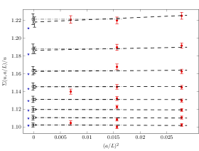
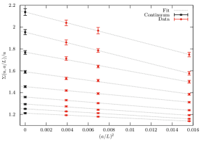
Figure 2: Continuum extrapolations of the lattice SSF of $\bar{g}^{2}_{{\rm SF},\nu=0}$ (left panel) and $\bar{g}^{2}_{\rm GF}$ (right panel), for different values of the couplings. The lattice data is shown in red while the black points are the continuum extrapolated results. For the details on the extrapolations, we refer to Dalla Brida et al. (2018) and Dalla Brida et al. (2017), respectively.

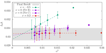
Figure 3: Determination of $L_{0}\Lambda\equiv\Lambda^{{N_{\rm f}}=3}_{{\rm SF},\nu=0}/\mu_{0}$ at different values of $\alpha\equiv\alpha_{{\rm SF},\nu}(\mu_{n})$. We compare the extraction in different schemes ($\nu=-0.5,0,0.3)$, and show a comparison with the final result Equation (13). As one can see, when the extraction is performed at high enough energies $(\alpha\approx 0.1)$, all schemes agree.

4.2 Low-Energy Running and Determination of $\mu_{0}/\mu_{\rm had}$

In order to express $\Lambda_{\overline{\rm MS}}^{{N_{\rm f}}=3}$ in physical units, we must link the technical scale $\mu_{0}$ with some experimentally accessible hadronic quantity. In order to keep systematic errors under control, we shall first relate $\mu_{0}$ with another finite-volume scale $\mu_{\rm had}={\rm O}(100\,{\rm MeV})$, and then relate this with some hadronic quantity. We do this in the following way. Through some dedicated simulations, we first relate $\bar{g}^{2}_{{\rm SF},\nu=0}(\mu_{0})$ with the GF coupling of Equation (11) at the scale $\mu_{0}/2$, obtaining: $\bar{g}^{2}_{\rm GF}(\mu_{0}/2)=2.6723(64)$ Dalla Brida et al. (2017). Then, similarly to what we did for the SF couplings, we compute the lattice SSF of the GF coupling for several values of $\bar{g}^{2}_{\rm GF}\approx 2-6.5$, and lattice sizes, $L/a=8-16$. The lattice SSFs are then extrapolated to the continuum, and a parametrization of the continuum SSF is obtained Dalla Brida et al. (2017). In this case, the continuum extrapolations are more delicate than in the case of the SF couplings, due to significantly larger discretization errors (cf. right panel of Figure 2). Nonetheless, a very good precision is attained for the final continuum results thanks to the high statistical accuracy of the GF coupling.

Having the (continuum) SSF, one can determine the non-perturbative $\beta$-function of the coupling. The exact relation between the two is obtained by noticing that:

$$\ln{\mu_{2}\over\mu_{1}}=\int_{\bar{g}_{\mathcal{O}}(\mu_{1})}^{\bar{g}_{\mathcal{O}}(\mu_{2})}{{\rm d}g\over\beta_{\mathcal{O}}(g)}\quad\Rightarrow\quad\log 2=-\int_{\sqrt{u}}^{\sqrt{\sigma_{\mathcal{O}}(u)}}{{\rm d}g\over\beta_{\mathcal{O}}(g)}\quad\text{where}\quad u=\bar{g}^{2}_{\mathcal{O}}(\mu).$$ (14)

The results for the non-perturbative $\beta$-function of the GF coupling are shown in the left panel of Figure 4, together with the results for the non-perturbative $\beta$-function of the SF coupling analogously obtained; a comparison with their (universal) LO and NLO predictions is also shown (cf. Equation (4)). Observe the peculiar behaviour of the non-perturbative $\beta$-function of the GF coupling, which lies very close to its LO result even at large values of the coupling, where $\alpha\approx 1$. Note, however, that, for most of the coupling range, we studied, the deviation from LO perturbation theory is statistically significant Dalla Brida et al. (2017). Only at values of $\alpha\approx 0.2$ do the non-perturbative results then start to approach their NLO prediction.

The $\beta$-function allows us to compute the ratio of energy scales corresponding to any two values of the coupling (cf. Equation (14)). Defining the technical scale $\mu_{\rm had}$ through a relatively large value of the GF coupling: $\bar{g}^{2}_{\rm GF}(\mu_{\rm had})=11.31$, Equation (14) and the non-perturbative results for $\beta_{\rm GF}$ give us Dalla Brida et al. (2017); Bruno et al. (2017):

$${\mu_{0}/\mu_{\rm had}}=21.86(42)\quad\Rightarrow\quad{\Lambda^{{N_{\rm f}}=3}_{\overline{\rm MS}}/\mu_{\rm had}}=1.729(57).$$ (15)

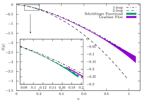
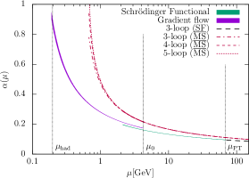
Figure 4: (Left): Non-perturbative $\beta$-functions in the GF and SF $(\nu=0)$ schemes determined in refs. Dalla Brida et al. (2017) and Dalla Brida et al. (2016, 2018), respectively. (Right): Running couplings of ${N_{\rm f}}=3$ QCD obtained from $\Lambda^{{N_{\rm f}}=3}_{\overline{\rm MS}}$ by integrating the non-perturbative $\beta$-functions Bruno et al. (2017).

4.3 Hadronic Matching and $\Lambda_{\overline{\rm MS}}^{{N_{\rm f}}=3}$

All that is left to do to determine $\Lambda_{\overline{\rm MS}}^{{N_{\rm f}}=3}$ is to relate the finite-volume scale $\mu_{\rm had}$ to some experimentally accessible quantity. This is best done by introducing a convenient intermediate reference scale, $\mu_{\rm ref}=1/\sqrt{8t_{0}}$ Bruno et al. (2017). The quantity $t_{0}$ corresponds to a specific flow time, which is implicitly defined by the flow energy density through the equation (cf. Equations (10)-(11)) Lüscher (2010):

$$t^{2}_{0}\,\langle E(t_{0},x)\rangle=0.3,\qquad E(t,x)=\hbox{$1\over 4$}G^{a}_{\mu\nu}(t,x)G^{a}_{\mu\nu}(t,x).$$ (16)

Note that differently from the case of the GF coupling, Equation (11), the expectation value appearing in this equation is the one of the theory in infinite space-time volume. Some of the nice features of the scale $\mu_{\rm ref}$ are that it can be determined very accurately in lattice QCD simulations and at a very modest computational effort. Moreover, theoretical arguments and numerical evidence show that it depends very little on the value of the quark masses which are simulated. This is a great advantage in performing extrapolations to physical quark masses when these are necessary. Of course, $\mu_{\rm ref}$ is not measurable in experiments, and its value in physical units must be determined by connecting it, through lattice QCD, to some experimentally accessible quantity. Once the value of $\mu_{\rm ref}$ in physical units is known, it is generally more convenient to express lattice quantities in terms of $\mu_{\rm ref}$ rather than directly in terms of an hadronic quantity (see e.g., Ref. Sommer (2014)). This is because usually the former can be more simply and accurately determined.

The value of $\mu_{\rm ref}$ in physical units was obtained in Ref. Bruno et al. (2017), to which we refer for any detail. In short, this was computed employing an extensive set of large volume simulations of ${N_{\rm f}}=3$ QCD Bruno et al. (2015), and a precise renormalization programme Dalla Brida et al. (2016, 2018), which allowed to determine, in the continuum, infinite volume limit, and for physical up, down and strange quark masses, the ratio: $f_{\pi K}/\mu_{\rm ref}$, where $f_{\pi K}=\hbox{$2\over 3$}(f_{K}+\hbox{$1\over 2$}f_{\pi})$ is a combination of pion and kaon decay constants. Using the PDG value for $f_{\pi K}$, one then arrives at: $\mu_{\rm ref}=478(6)\,{\rm MeV}$. In fact, for technical reasons, rather than using the value of $\mu_{\rm ref}$ at physical quark masses, we shall use $\mu_{\rm ref}$ evaluated for equal up, down, and strange quark masses, close to their average physical value Bruno et al. (2017); we indicate this "new" scale as $\mu^{*}_{\rm ref}=1/\sqrt{8t^{*}_{0}}$. Its value in physical units can be determined once again through lattice QCD simulations by relating $\mu^{*}_{\rm ref}$ to $f_{\pi K}$ or $\mu_{\rm ref}$. Doing this one obtains: $\mu_{\rm ref}^{*}=478(7)\,{\rm MeV}$ Bruno et al. (2015), which actually shows how $\mu_{\rm ref}$ depends very little on the value of the quark masses. Having this result, we can obtain $\Lambda_{\overline{\rm MS}}^{{N_{\rm f}}=3}$ in physical units by computing the ratio $\mu^{*}_{\rm ref}/\mu_{\rm had}$ (cf. Equation (12)). Given the large volume results for $a\mu^{*}_{\rm ref}$ at several values of the lattice spacing $a$ Bruno et al. (2017), this can be determined with modest computational effort from a small set of lattice QCD simulations of the SF Bruno et al. (2017). The result we obtain is:

$$\mu^{*}_{\rm ref}/\mu_{\rm had}=2.428(18)\quad\Rightarrow\quad\Lambda^{{N_{\rm f}}=3}_{\overline{\rm MS}}=341(12)\,{\rm MeV}.$$ (17)

From $\Lambda^{{N_{\rm f}}=3}_{\overline{\rm MS}}$ and the non-perturbative $\beta$-functions of the SF and GF couplings, one can reconstruct the non-perturbative running of the couplings over the whole range of energy we covered, which goes from $\mu_{\rm had}\approx 200\,{\rm MeV}$ to $\mu_{\rm PT}=16\mu_{0}\approx 70\,{\rm GeV}$. The result is shown in the right panel of Figure 4.

4.4 Perturbative Decoupling and $\alpha_{s}$

To arrive at $\alpha_{s}(m_{Z})$, one needs $\Lambda_{\overline{\rm MS}}^{{N_{\rm f}}=5}$. The way we obtain this is to take as an input the non-perturbatively determined $\Lambda_{\overline{\rm MS}}^{{N_{\rm f}}=3}$ of Equation (17), and use perturbation theory to compute the ratio $\Lambda_{\overline{\rm MS}}^{{N_{\rm f}}=5}/\Lambda_{\overline{\rm MS}}^{{N_{\rm f}}=3}$ Bruno et al. (2017). More precisely, assuming a perturbative decoupling of the charm and bottom quarks, the couplings of QCD with ${N_{\rm f}}=5$ and ${N_{\rm f}}=3$ quark-flavours are matched using perturbation theory at the charm and bottom quark-mass thresholds. This matching then translates into a perturbative relation between the $\Lambda$-parameters of the two theories (see refs. Athenodorou et al. (2018); Bruno et al. (2015) for the details). The reliability and accuracy of perturbation theory in this step has been recently addressed in a systematic way in Ref. Athenodorou et al. (2018). The conclusion of this study is that perturbation theory is expected to be reliable in predicting this ratio of $\Lambda$-parameters to a sub-percent accuracy. Since our determination of $\Lambda_{\overline{\rm MS}}^{{N_{\rm f}}=3}$ has a precision of about 3%, we expect that the non-perturbative effects in the decoupling of the charm and bottom quarks are negligible in practice. In addition, the effect of neglecting the charm (and thus bottom) quark contributions to dimensionless ratios of low-energy quantities, which are relevant for the determination of the physical scale of the lattice simulations (cf. Section 4.3), has been estimated to be well-below the percent level Bruno et al. (2015); Knechtli et al. (2017). It is thus also safe to establish the connection with hadronic physics using lattice QCD with ${N_{\rm f}}=3$ quark-flavours. Given these observations, we conclude:

$$\Lambda^{{N_{\rm f}}=3}_{\overline{\rm MS}}\to\Lambda^{{N_{\rm f}}=5}_{\overline{\rm MS}}=215(10)(3)\,{\rm MeV}\quad\Rightarrow\quad\alpha^{({N_{\rm f}}=5)}_{\overline{\rm MS}}(m_{Z})=0.11852(80)(25).$$ (18)

The second error in $\Lambda_{\overline{\rm MS}}^{{N_{\rm f}}=5}$, then propagated to $\alpha_{s}$, comes from an estimate (within perturbation theory) of the truncation of the perturbative expansion to 4-loop order in computing $\Lambda_{\overline{\rm MS}}^{{N_{\rm f}}=5}/\Lambda_{\overline{\rm MS}}^{{N_{\rm f}}=3}$ Bruno et al. (2017).

5 Conclusions and Outlook

In this contribution, we presented a sub-percent precision determination of $\alpha_{s}$ by means of lattice QCD. Employing carefully chosen finite-volume couplings and a step-scaling strategy, we overcame the shortcomings of a naive application of lattice QCD to this problem. This allowed us to keep all systematic uncertainties well-under control. We determined the $\Lambda$-parameter of ${N_{\rm f}}=3$ QCD by studying the non-perturbative running of the finite-volume couplings from a few hundred MeV up to O(100 GeV), where the use of perturbation theory was carefully studied. We then computed $\Lambda_{\overline{\rm MS}}^{{N_{\rm f}}=5}$ employing a perturbative estimate for $\Lambda_{\overline{\rm MS}}^{{N_{\rm f}}=5}/\Lambda_{\overline{\rm MS}}^{{N_{\rm f}}=3}$, which has been shown to be accurate within our precision. From our result for $\Lambda_{\overline{\rm MS}}^{{N_{\rm f}}=5},$ we finally obtained $\alpha^{({N_{\rm f}}=5)}_{\overline{\rm MS}}(m_{Z})=0.11852(84)$, which has an error of $\approx 0.7\%$. Our result compares well with the current PDG world average: $\alpha^{\text{PDG '18}}_{\overline{\rm MS}}(m_{Z})=0.1181(11)$.

Studying the error budget of our determination, we can say that the dominant source of uncertainty is statistical, and comes from the computation of the non-perturbative running of the couplings. There is thus room for improvement in this direction. In addition, one might want to consider including explicitly the charm quark in the calculation, in order to rely even less on perturbative information. In conclusion, a determination of $\alpha_{s}$ with 0.5% accuracy can be foreseen.

This research received no external funding.