Dynamically generated magnetic moment in the Wigner-function formalism

Abstract

We study how the mass and magnetic moment of the quarks are dynamically generated in nonequilibrium quark matter. We derive the equal-time transport and constraint equations for the quark Wigner function in a magnetized quark model and solve them in the semi-classical expansion. The quark mass and magnetic moment are self-consistently coupled to the Wigner function and controlled by the kinetic equations. While the quark mass is dynamically generated at the classical level, the quark magnetic moment is a pure quantum effect, induced by the quark spin interaction with the external magnetic field.

The intrinsic magnetic moment of an electron is related to its spin by ${\bf m}_{s}=g\mu_{B}{\bf s}$, where $\mu_{B}=e/(2m)$ is Bohr’s magneton, with $e$ and $m$ being the electron charge and mass, $g$ the Lande factor, and ${\bf s}$ the electron spin angular momentum, respectively. Dirac theory predicts $g=2$ in the non-relativistic limit, but this result was later challenged by many refined experimental measurements, showing a larger $g$ factor. Schwinger calculated the first-order radiative correction to ${\bf m}_{s}$ from the electron-photon interaction schwinger . The one-loop contribution to the fermion self-energy was taken into account in a weak magnetic field, which leads to an anomalous magnetic moment, reflected in a correction to the $g$ factor of order $\sim(g-2)/2=\alpha/(2\pi)$, where $\alpha$ is the fine-structure constant. Higher-order radiative corrections to $g$ have subsequently been considered high ; high1 , resulting in a series in powers of $\alpha/\pi$. These corrections are in excellent agreement with experimental data. In an external magnetic field ${\bf B}$, the anomalous magnetic moment affects the electron energy in the lowest Landau level by turning the mass into $m^{2}_{eff}\simeq m^{2}+(g-2)eB/2$. In the case of massless quantum electrodynamics (QED), the anomalous magnetic moment cannot be described through Schwinger’s perturbative approach, and chiral symmetry breaking will dynamically generate an anomalous magnetic moment chiralmag2 .

The anomalous magnetic moment in QED is a fundamental phenomenon in gauge field theory. It should happen also for quarks in quantum chromodynamics (QCD) chiralmag1 ; chiralmag3 . Considering its non-Abelian and non-perturbative properties, it becomes much more difficult to directly investigate the quantum fluctuations in QCD, and effective models without gauge fields, like chiral perturbation theory cpt1 ; cpt2 at the hadron level and the Nambu–Jona-Lasinio model njl1 ; njl2 ; njl3 ; njl4 at the quark level, are used to calculate the properties of, and spontaneous symmetry breaking in, strong-interaction systems. For instance, $U(1)_{A}$ symmetry breaking and spontaneous chiral symmetry breaking in vacuum and their restoration in medium are investigated for thermal equilibrium systems in an $SU(3)$ linear sigma model jiang and for non-equilibrium systems in an NJL model guo . In the chiral limit, the quark magnetic moment is closely related to the chiral symmetry of QCD chiralmag2 ; chiralmag1 ; chiralmag3 , which is spontaneously broken in vacuum through the chiral condensate $\langle\bar{\psi}\psi\rangle$ or the dynamical quark mass $m_{q}$. Recent lattice-QCD simulations lattice1 ; lattice2 ; lattice3 show that the breaking is further enhanced in an external magnetic field. Since the constituent quark and anti-quark of the chiral condensate have opposite spins and opposite charges, the pair’s magnetic moment will align with the magnetic field, leading to a condensate $\langle\bar{\psi}\gamma_{1}\gamma_{2}\tau_{3}\psi\rangle$ in the ground state. Therefore, the chiral condensate will inexorably provide the quasi-particles with both a dynamical mass and a dynamical magnetic moment. The tensor condensate is discussed at finite temperature in a one-flavor NJL model in the lowest-Landau-level approximation in a magnetic field in Ref. amm2 , and the discussion is extended to a two-flavor NJL model at finite density in Ref. amm3 .

The only possibility to realize a magnetic field in the laboratory which is comparable in strength with typical QCD energy scales is via high-energy heavy-ion collisions. For heavy-ion collisions at the Relativistic Heavy-Ion Collider and the Large Hadron Collider, the magnetic field can reach a magnitude of $eB\sim m_{\pi}^{2}$ b2 ; b3 ; b4 ; b5 , however, only for a very short time in the early stage of the collision. Considering that the colliding system is initially in a state far from equilibrium, one should study the magnetic moment induced by chiral symmetry breaking in the framework of quantum transport theory. One possible way to formulate this theory is the Wigner-function formalism qt1 ; qt2 ; qt3 ; qt4 ; qt5 . In this Letter, we study the space-time dependent magnetic moment dynamically generated in quark matter, by applying equal-time transport theory qt4 ; qt5 to an $SU(2)$ NJL model. We first calculate the temperature dependence of the dynamical magnetic moment in the equilibrium case, and then focus on the classical and quantum kinetic equations for the dynamical quark mass and the dynamical magnetic moment.

The Lagrangian of the magnetized $SU(2)$ NJL model with a tensor interaction reads njl1 ; njl2 ; njl3 ; njl4

$${\cal L}=\bar{\psi}\left(i\gamma^{\mu}{\cal D}_{\mu}-m_{0}\right)\psi+G_{s}\left[\left(\bar{\psi}\psi\right)^{2}+\left(\bar{\psi}i\gamma_{5}{\bf\tau}\psi\right)^{2}\right]-{G_{t}\over 4}\left[\left(\bar{\psi}\gamma_{\mu}\gamma_{\nu}{\bf\tau}\psi\right)^{2}+\left(\bar{\psi}i\gamma_{5}\gamma_{\mu}\gamma_{\nu}\psi\right)^{2}\right]\;,$$ (1)

where the covariant derivative ${\cal D}_{\mu}=\partial_{\mu}+iQA_{\mu}$ couples quarks with electric charge $Q=\mathrm{diag}(Q_{u},Q_{d})=\mathrm{diag}(2e/3,-e/3)$ to an external magnetic field ${\bf B}=(0,0,B)$ pointing in the $x_{3}$-direction through the potential $A_{\mu}=(0,0,Bx_{1},0)$. The coupling constant $G_{s}$ in the scalar/pseudo-scalar channel controls the spontaneous chiral symmetry breaking, which generates a dynamical quark mass, and the coupling constant $G_{t}$ in the tensor/pseudo-tensor channels controls the spin-spin interaction, which leads to a dynamical magnetic moment. Here, $m_{0}$ is the current quark mass characterizing the explicit chiral symmetry breaking. In the following, we focus on the chiral limit with $m_{0}=0$. When the magnetic field is turned on, the chiral symmetry $SU(2)_{L}\otimes SU(2)_{R}$ is reduced to $U(1)_{L}\otimes U(1)_{R}$. Throughout the paper we use the notation $\mathbf{a}=(a_{1},a_{2},a_{3})$ for 3-vectors and $a^{\mu}=(a_{0},\mathbf{a})$ for 4-vectors.

The order parameter for the chiral phase transition is the chiral condensate $\langle\bar{\psi}\psi\rangle$ or the dynamical quark mass $m_{q}=-2G_{s}\langle\bar{\psi}\psi\rangle$. In a magnetic field, we also introduce a tensor condensate $F_{3}=-iG_{t}\langle\bar{\psi}\gamma_{1}\gamma_{2}\tau_{3}\psi\rangle$, which plays the role of the dynamical magnetic moment of the quarks. Here we consider the dynamical magnetic moment along the direction of the magnetic field. In mean-field approximation, the Lagrangian of the model becomes

$${\cal L}=\bar{\psi}\left(i\gamma^{\mu}{\cal D}_{\mu}-m_{q}-iF_{3}\gamma_{1}\gamma_{2}\tau_{3}\right)\psi-\frac{m_{q}^{2}}{4G_{s}}-\frac{F_{3}^{2}}{2G_{t}}\;.$$ (2)

By taking the quark propagator in a magnetic field in the Ritus scheme ritus1 ; ritus2 ; ritus3 , the thermodynamical potential of the quark system contains a mean-field part and a quasi-quark part,

$$\Omega = \frac{m_{q}^{2}}{4G_{s}}+\frac{F_{3}^{2}}{2G_{t}}+\Omega_{q}\;,$$ (3)

$$\Omega_{q} = -N_{c}\sum_{f,\eta,n}\int\frac{dp_{3}}{2\pi}\frac{|Q_{f}B|}{2\pi}\left[\epsilon_{f\eta n}-2T\ln g(-\epsilon_{f\eta n})\right]\;,$$

where $g(x)=\left(1+e^{x/T}\right)^{-1}$ is the Fermi-Dirac distribution, $\epsilon_{f\eta n}=\sqrt{p^{2}_{3}+\left(\sqrt{m_{q}^{2}+2n|Q_{f}B|}+\eta F_{3}\right)^{2}}$ is the quark energy of flavor $f=u,d$, and the summation over the discrete Landau energy levels runs over $n=0,1,2,\ldots$ for $\eta=+$ and over $n=1,2,3,\ldots$ for $\eta=-$. The spectrum of the quasi-quarks in Landau levels $n>0$ exhibits a Zeeman splitting ($\eta=\pm$) due to the tensor condensate $F_{3}$. Therefore, we always use the term “dynamical magnetic moment” for the tensor condensate $F_{3}$. No splitting is present in the $n=0$ mode, since the fermion in the lowest Landau level has only one spin projection. The dynamical quark mass and magnetic moment are self-consistently determined by the minimum of the thermodynamic potential,

$${\partial\Omega\over\partial m_{q}}=0\;,\ \ \ \ {\partial\Omega\over\partial F_{3}}=0\;.$$ (4)

Because of the contact interaction among quarks, the NJL model is non-renormalizable, and it is necessary to introduce a regularization scheme to remove the ultraviolet divergences of the momentum integrals. To guarantee the law of causality in a magnetic field, we take a covariant Pauli-Villars regularization as explained in detail in Ref. mao . The two parameters of the model in the chiral limit, namely the quark coupling constant $G_{s}=3.52$ GeV^-2 and the Pauli-Villars mass parameter $\Lambda=1127$ MeV are fixed by fitting the pion decay constant $f_{\pi}=93$ MeV and the chiral condensate $\langle\bar{\psi}\psi\rangle=(-250\ \text{MeV})^{3}$ in vacuum at $T=B=0$. The coupling constant $G_{t}$ in the tensor channel is treated as a free parameter.

Let us first consider the lowest-Landau-level approximation. In this case, the two gap equations simplify considerably and become

$$\frac{m_{q}}{2G_{s}}+(m_{q}+F_{3})I_{0}=0\;,$$

$$\frac{F_{3}}{G_{t}}+(m_{q}+F_{3})I_{0}=0\;,$$ (5)

with

$$I_{0}=-N_{c}\frac{|eB|}{\left(2\pi\right)^{2}}\int\frac{d{p_{3}}}{\epsilon_{3}}\left[1-2g\left(\epsilon_{3}\right)\right]\;.$$ (6)

The quark energy $\epsilon_{f\eta n}$ becomes flavor-independent in the lowest Landau level with $n=0$ and $\eta=+$, $\epsilon_{3}=\sqrt{p^{2}_{3}+(m_{q}+F_{3})^{2}}$.

From the two gap equations (Dynamically generated magnetic moment in the Wigner-function formalism), we readily observe that the dynamical magnetic moment $F_{3}$ and the dynamical quark mass $m_{q}$ are proportional to each other,

$$\frac{F_{3}}{m_{q}}=\frac{G_{t}}{2G_{s}},$$ (7)

independent of temperature, magnetic field, and the regularization scheme used. Once quarks acquire a dynamical mass, they should also acquire a dynamical magnetic moment. This effect has also been reported in massless QED and in a one-flavor NJL model chiralmag2 ; chiralmag1 ; amm2 . The constituent quark and anti-quark forming the chiral condensate have opposite spins and opposite charges, the magnetic moment of the pair is then aligned with the external magnetic field. This leads to a dynamical magnetic moment $F_{3}$ in the ground state. From the view of symmetry, once the chiral symmetry is dynamically broken, there is no symmetry protecting the dynamical magnetic moment, because a nonvanishing value of the latter breaks exactly the same symmetry.

Including all Landau levels, the proportionality (7) between $F_{3}$ and $m_{q}$ no longer holds exactly, but is still approximately satisfied, see the numerical calculations of the original gap equations (4) shown in Fig. 1. With increasing temperature, the scalar and tensor condensates continuously melt and approach zero at the same critical temperature, and $F_{3}$ remains zero in the chirally restored phase, characterized by $m_{q}=0$. This proves the original idea that the dynamical magnetic moment is induced by chiral symmetry breaking. With increasing coupling strength $G_{t}$ in the tensor channel, $F_{3}$ is significantly enhanced but $m_{q}$ changes only slightly. While there is still an approximate proportionality between $F_{3}$ and $m_{q}$, the proportionality constant in the full calculation is much smaller than $G_{t}/(2G_{s})$ in the lowest-Landau-level approximation, see the lower panel of Fig. 1. This is due to the different contributions from the higher Landau levels to $m_{q}$ and $F_{3}$. The quarks in higher Landau levels participate in the scalar condensate in the same way as the quark in the lowest Landau level and therefore enhance the dynamical quark mass considerably. However, the quark in the lowest Landau level constitutes the major contribution to the dynamical magnetic moment due to its single spin projection. Including higher Landau levels, the dynamical magnetic moment is only slightly changed because of the cancellation between the two spin projections of the quarks in higher Landau levels.

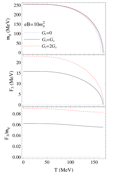
Figure 1: The dynamical quark mass, dynamical magnetic moment, and their ratio as functions of temperature in a constant magnetic field $eB=10\ m^{2}_{\pi}$ for different values of the coupling strength $G_{t}$ in the tensor channel.

Apart from the nonzero coupling $G_{t}$, the other necessary condition for a nonvanishing dynamical magnetic moment is a nonzero external magnetic field. When the magnetic field is turned off, the gap equations (4) become

$$m_{q}\left\{1+2G_{s}N_{c}N_{f}\sum_{\eta}\int\frac{d^{3}{\bf p}}{(2\pi)^{3}}\frac{1+\eta F_{3}/\epsilon_{\perp}}{\epsilon_{\eta}}\left[g(\epsilon_{\eta})-g(-\epsilon_{\eta})\right]\right\} = 0\;,$$

$$F_{3}+G_{t}N_{c}N_{f}\sum_{\eta}\int\frac{d^{3}{\bf p}}{(2\pi)^{3}}\frac{F_{3}+\eta\epsilon_{\perp}}{\epsilon_{\eta}}\left[g(\epsilon_{\eta})-g(-\epsilon_{\eta})\right] = 0\;,$$ (8)

with quark energy $\epsilon_{\eta}=\sqrt{p^{2}_{3}+(\epsilon_{\perp}+\eta F_{3})^{2}}$ and transverse energy $\epsilon_{\perp}=\sqrt{p^{2}_{1}+p^{2}_{2}+m_{q}^{2}}$. The solution of the gap equations is $F_{3}=0$ in both the chiral symmetry broken and restored phases. Physically, without magnetic field, the randomly oriented quark spins lead to a vanishing dynamical magnetic moment in the ground state.

As the magnetic field is turned on, a nonzero dynamical magnetic moment is induced and increases with magnetic field. Figure 2 shows the dynamical magnetic moment as a function of magnetic field at zero and finite temperature for different values of the tensor coupling $G_{t}$. The dynamical magnetic moment is linearly proportional to the external magnetic field at zero temperature, analogously to the anomalous magnetic moment in Schwinger’s calculation in QED schwinger . The linear relation is broken by the thermal motion of quarks, see the lower panel of Fig. 2.

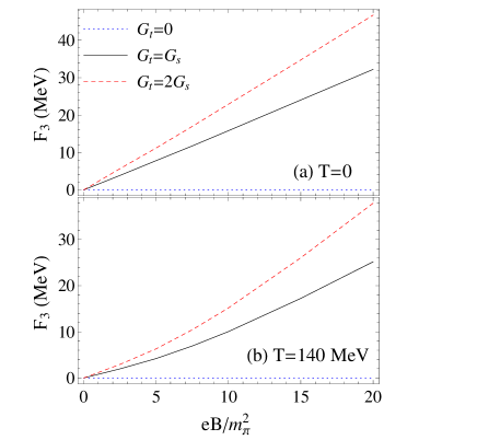
Figure 2: The dynamical magnetic moment as a function of magnetic field at different temperature and different values for the coupling constant $G_{t}$ in the tensor channel.

We now turn to non-equilibrium systems. For systems in a sufficiently strong magnetic field, like matter created in the early stages of relativistic heavy-ion collisions, the calculation in the framework of finite-temperature field theory fails, and we need to treat the dynamical evolution of the system in the framework of transport theory. In the following, we consider the dynamical evolution of the quark mass and magnetic moment in an external electromagnetic field by using the Wigner-function formalism applied to the NJL model with a tensor interaction. To appropriately treat the quantum fluctuations, especially the off-shell effect, order by order, we apply equal-time quantum transport theory, which has been successfully developed in QED qt3 ; qt4 ; qt5 . We will see clearly that the dynamical quark mass is generated at the classical level, but the magnetic moment arises from quantum fluctuations.

The covariant quark Wigner function in a gauge field theory is defined as

$$W(x,p)=\int d^{4}ye^{ipy}\left\langle\psi(x_{+})e^{iQ\int^{1/2}_{-{1/2}}dsA(x+sy)y}\bar{\psi}(x_{-})\right\rangle\;,$$ (9)

where the exponential function is the gauge link between the two points $x_{-}=x-y/2$ and $x_{+}=x+y/2$, which guarantees gauge invariance qt3 , and the symbol $\langle...\rangle$ means ensemble average of the Wigner operator. For external (classical) gauge fields, the link factor can be moved out of the ensemble average.

From the mean-field Lagrangian (2) in the chiral limit, we obtain the Dirac equation for the quark field,

$$\left(i\gamma^{\mu}{\cal D}_{\mu}-m_{q}-iF_{3}\gamma_{1}\gamma_{2}\tau_{3}\right)\psi=0\;.$$ (10)

Again, we consider here the dynamical magnetic moment $F_{3}$ along the direction of the magnetic field.

Using the Dirac equation, we derive the generalized Vasak-Gyulassy-Elze equation qt3 for the quark Wigner function for flavor $f$,

$$\left(\gamma^{\mu}K_{\mu}-M+K_{3}\gamma_{1}\gamma_{2}\right)W=0\;,$$ (11)

with the operators

$$K_{\mu} = \Pi_{\mu}+\frac{i}{2}\hbar D_{\mu}\;,$$

$$\Pi_{\mu} = p_{\mu}-i\hbar Q_{f}\int^{1/2}_{-1/2}dssF_{\mu\nu}(x-i\hbar s\partial_{p})\partial^{\nu}_{p}\;,$$

$$D_{\mu} = \partial_{\mu}-Q_{f}\int^{1/2}_{-1/2}dsF_{\mu\nu}(x-i\hbar s\partial_{p})\partial^{\nu}_{p}\;,$$ (12)

related to the electromagnetic interaction,

$$M = M_{1}+iM_{2}\;,$$

$$M_{1} = \cos\left(\frac{\hbar}{2}\partial_{x}\cdot\partial_{p}\right)m_{q}(x)\;,$$

$$M_{2} = -\sin\left(\frac{\hbar}{2}\partial_{x}\cdot\partial_{p}\right)m_{q}(x)\;,$$ (13)

related to the dynamical quark mass controlled by the scalar interaction, and

$$K_{3} = F_{o}+iF_{e}\;,$$

$$F_{e} = -\text{sgn}(Q_{f})\cos\left(\frac{\hbar}{2}\partial_{x}\cdot\partial_{p}\right)F_{3}(x)\;,$$

$$F_{o} = -\text{sgn}(Q_{f})\sin\left(\frac{\hbar}{2}\partial_{x}\cdot\partial_{p}\right)F_{3}(x)\;,$$ (14)

related to the dynamical magnetic moment controlled by the tensor interaction. We have explicitly exhibited the $\hbar$-dependence in order to be able to discuss the semi-classical expansion of the kinetic equation in the following. Considering that the Wigner function defined through Eq. (9) is a $4\times 4$ matrix in Dirac space and in general not a real-valued function, its physical meaning becomes clear only after the spinor decomposition qt3

$$W=\frac{1}{4}\left(F+i\gamma_{5}P+\gamma_{\mu}V^{\mu}+\gamma_{\mu}\gamma_{5}A^{\mu}+\frac{1}{2}\sigma_{\mu\nu}S^{\mu\nu}\right)\;.$$ (15)

To compare the covariant Wigner function $W(x,p)$ defined in $4-$dimensional momentum space with the observable physics densities such as the number density defined in $3-$dimensional momentum space, we introduce the equal-time Wigner function ${\cal W}(x,{\bf p})$ by integrating the covariant Wigner function $W(x,p)$ over the energy $p_{0}$ and furthermore apply the corresponding spinor decomposition,

$${\cal W} = \int dp_{0}W\gamma_{0}$$ (16)

$$= \frac{1}{4}\left(f_{0}+\gamma_{5}f_{1}-i\gamma_{0}\gamma_{5}f_{2}+\gamma_{0}f_{3}+\gamma_{5}\gamma_{0}{\bf\gamma}\cdot{\bf g}_{0}+\gamma_{0}{\bf\gamma}\cdot{\bf g}_{1}-i{\bf\gamma}\cdot{\bf g}_{2}-\gamma_{5}{\bf\gamma}\cdot{\bf g}_{3}\right)\;.$$

The physical meaning of the spinor components of the equal-time Wigner function $f_{i}(x,{\bf p})$ and ${\bf g}_{i}(x,{\bf p})$, $i=0,1,2,3$, is discussed in detail in Ref. qt4 in QED. For instance, $f_{0}$ is the number density, ${\bf g}_{0}$ the spin density, and ${\bf g}_{1}$ the number current.

Since the kinetic equation (11) is a complete equation, when taking the spinor decomposition (15) it becomes $16$ transport equations with derivative $D_{\mu}$ plus $16$ constraint equations with operator $\Pi_{0}$ for the spinor components $F,P,V^{\mu},A^{\mu}$, and $S^{\mu\nu}$. The former controls the dynamical evolution of the $16$ components in phase space, and the latter is the quantum extension of the classical on-shell condition qt5 . By taking the energy integration of these kinetic equations, we obtain a set of transport equations for the spinor components of the equal-time Wigner function,

$${\hbar\over 2}\left(d_{0}f_{0}+{\bf d}\cdot{\bf g}_{1}\right)-m_{2}f_{3}-f_{o}{\bf g}_{3}\cdot{\bf e}_{3}=0\;,$$

$${\hbar\over 2}\left(d_{0}f_{1}+{\bf d}\cdot{\bf g}_{0}\right)+m_{1}f_{2}-f_{e}{\bf g}_{2}\cdot{\bf e}_{3}=0\;,$$

$${\hbar\over 2}d_{0}f_{2}+{\bf\pi}\cdot{\bf g}_{3}-m_{1}f_{1}+f_{e}{\bf g}_{1}\cdot{\bf e}_{3}=0\;,$$

$${\hbar\over 2}d_{0}f_{3}-{\bf\pi}\cdot{\bf g}_{2}-m_{2}f_{0}-f_{o}{\bf g}_{0}\cdot{\bf e}_{3}=0\;,$$

$${\hbar\over 2}\left(d_{0}{\bf g}_{0}+{\bf d}f_{1}\right)-{\bf\pi}\times{\bf g}_{1}-m_{2}{\bf g}_{3}-f_{e}{\bf g}_{3}\times{\bf e}_{3}-f_{o}f_{3}\mathbf{e}_{3}=0\;,$$

$${\hbar\over 2}\left(d_{0}{\bf g}_{1}+{\bf d}f_{0}\right)-{\bf\pi}\times{\bf g}_{0}+m_{1}{\bf g}_{2}+f_{o}{\bf g}_{2}\times{\bf e}_{3}-f_{e}f_{2}\mathbf{e}_{3}=0\;,$$

$${\hbar\over 2}\left(d_{0}{\bf g}_{2}+{\bf d}\times{\bf g}_{3}\right)+{\bf\pi}f_{3}-m_{1}{\bf g}_{1}-f_{o}{\bf g}_{1}\times{\bf e}_{3}+f_{e}f_{1}\mathbf{e}_{3}=0\;,$$

$${\hbar\over 2}\left(d_{0}{\bf g}_{3}-{\bf d}\times{\bf g}_{2}\right)-{\bf\pi}f_{2}-m_{2}{\bf g}_{0}-f_{e}{\bf g}_{0}\times{\bf e}_{3}-f_{o}f_{0}\mathbf{e}_{3}=0\;,$$ (17)

and a set of constraint equations,

$$V_{0}^{\prime}+\pi_{0}f_{0}-{\bf\pi}\cdot{\bf g}_{1}-m_{1}f_{3}+f_{e}{\bf g}_{3}\cdot{\bf e}_{3}=0\;,$$

$$A_{0}^{\prime}-\pi_{0}f_{1}+{\bf\pi}\cdot{\bf g}_{0}+m_{2}f_{2}+f_{o}{\bf g}_{2}\cdot{\bf e}_{3}=0\;,$$

$$P^{\prime}+\pi_{0}f_{2}+{\hbar\over 2}{\bf d}\cdot{\bf g}_{3}+m_{2}f_{1}+f_{o}{\bf g}_{1}\cdot{\bf e}_{3}=0\;,$$

$$F^{\prime}+\pi_{0}f_{3}-{\hbar\over 2}{\bf d}\cdot{\bf g}_{2}-m_{1}f_{0}+f_{e}{\bf g}_{0}\cdot{\bf e}_{3}=0\;,$$

$${\bf A}^{\prime}-\pi_{0}{\bf g}_{0}+{\hbar\over 2}{\bf d}\times{\bf g}_{1}+{\bf\pi}f_{1}+m_{1}{\bf g}_{3}+f_{o}{\bf g}_{3}\times{\bf e}_{3}-f_{e}f_{3}\mathbf{e}_{3}=0\;,$$

$${\bf V}^{\prime}+\pi_{0}{\bf g}_{1}-{\hbar\over 2}{\bf d}\times{\bf g}_{0}-{\bf\pi}f_{0}-m_{2}{\bf g}_{2}-f_{e}{\bf g}_{2}\times{\bf e}_{3}-f_{o}f_{2}\mathbf{e}_{3}=0\;,$$

$$S_{0i}^{\prime}{\bf e}_{i}-\pi_{0}{\bf g}_{2}+{\bf\pi}\times{\bf g}_{3}-{\hbar\over 2}{\bf d}f_{3}-m_{2}{\bf g}_{1}-f_{e}{\bf g}_{1}\times{\bf e}_{3}-f_{o}f_{1}\mathbf{e}_{3}=0\;,$$

$$S_{jk}^{\prime}\epsilon^{ijk}{\bf e}_{i}+2\pi_{0}{\bf g}_{3}+2{\bf\pi}\times{\bf g}_{2}-\hbar{\bf d}f_{2}-2m_{1}{\bf g}_{0}-f_{o}{\bf g}_{0}\times{\bf e}_{3}+f_{e}f_{0}\mathbf{e}_{3}=0\;,$$ (18)

where $\Gamma^{\prime}(x,{\bf p})=\int dp_{0}p_{0}\Gamma(x,p)\ (\Gamma=F,P,V^{\mu},A^{\mu},S^{\mu\nu})$ are the first-order energy moments of the covariant Wigner function, ${\bf e}_{1},{\bf e}_{2}$, and ${\bf e}_{3}$ are the unit vectors along the Cartesian coordinates $x_{1},x_{2}$, and $x_{3}$ in coordinate space, and the equal-time operators related to the quark electromagnetic, scalar, and tensor interactions are the energy integrals of the corresponding covariant operators,

$$d_{0} = \partial_{t}+Q_{f}\int^{1/2}_{-1/2}ds\ {\bf E}({\bf x}+i\hbar s{\bf\nabla}_{p},t)\cdot{\bf\nabla}_{p}\;,$$

$${\bf d} = {\bf\nabla}+Q_{f}\int^{1/2}_{-1/2}ds\ {\bf B}({\bf x}+i\hbar s{\bf\nabla}_{p},t)\times{\bf\nabla}_{p}\;,$$

$$\pi_{0} = i\hbar Q_{f}\int^{1/2}_{-1/2}ds\ s{\bf E}({\bf x}+i\hbar s{\bf\nabla}_{p},t)\cdot{\bf\nabla}_{p}\;,$$

$${\bf\pi} = {\bf p}-i\hbar Q_{f}\int^{1/2}_{-1/2}ds\ s{\bf B}({\bf x}+i\hbar s{\bf\nabla}_{p},t)\times{\bf\nabla}_{p}\;,$$

$$m_{1} = \cos\left({\hbar\over 2}{\bf\nabla}\cdot{\bf\nabla}_{p}\right)m_{q}(x)\;,$$

$$m_{2} = \sin\left({\hbar\over 2}{\bf\nabla}\cdot{\bf\nabla}_{p}\right)m_{q}(x)\;,$$

$$f_{e} = -\text{sgn}(Q_{f})\cos\left({\hbar\over 2}{\bf\nabla}\cdot{\bf\nabla}_{p}\right)F_{3}(x)\;,$$

$$f_{o} = \text{sgn}(Q_{f})\sin\left({\hbar\over 2}{\bf\nabla}\cdot{\bf\nabla}_{p}\right)F_{3}(x)\;.$$ (19)

Here we have replaced the field strength tensor $F_{\mu\nu}(x)$ by the electric and magnetic fields ${\bf E}(x)$ and ${\bf B}(x)$. Note that the energy moment $\int dp_{0}p_{0}W(x,p)\gamma_{0}$ in the constraint equations is in general independent of the equal-time Wigner function ${\cal W}(x,{\bf p})$ due to the quantum off-shell effect of particle transport in the medium qt5 . Only in the classical case, any order energy moment can be expressed as $\int dp_{0}p_{0}^{n}W(x,p)\gamma_{0}=\omega_{\bf p}^{n}{\cal W}(x,{\bf p}),\,n=0,1,2,\ldots$, in terms of the quasi-particle energy $\omega_{\bf p}$ and the equal-time Wigner function due to the classical on-shell condition $\delta(p_{0}-\omega_{\bf p})$.

Using the definitions of the scalar and tensor condensates $m_{q}=-2G_{s}\langle\bar{\psi}\psi\rangle=-2G_{s}\langle\bar{\psi}_{u}\psi_{u}+\bar{\psi}_{d}\psi_{d}\rangle$ and $F_{3}=-iG_{t}\langle\bar{\psi}\gamma_{1}\gamma_{2}\tau_{3}\psi\rangle=-iG_{t}\langle\bar{\psi}_{u}\gamma_{1}\gamma_{2}\psi_{u}-\bar{\psi}_{d}\gamma_{1}\gamma_{2}\psi_{d}\rangle$, these quantities can be expressed in terms of the Wigner function,

$$m_{q}(x)=-2G_{s}\int\frac{d^{3}{\bf p}}{(2\pi)^{3}}\left[f_{3u}(x,{\bf p})+f_{3d}(x,{\bf p})\right]\;,$$

$$F_{3}(x)=-G_{t}\int\frac{d^{3}{\bf p}}{(2\pi)^{3}}\left[{\bf g}_{3u}(x,{\bf p})-{\bf g}_{3d}(x,{\bf p})\right]\cdot{\bf e}_{3}\;.$$ (20)

This shows clearly the physics of the spinor components $f_{3}$ and ${\bf g}_{3}$: they are the source of the quark mass and the quark magnetic moment, respectively, and are then called mass density and magnetic-moment density. By solving the kinetic equations (Dynamically generated magnetic moment in the Wigner-function formalism) and (Dynamically generated magnetic moment in the Wigner-function formalism), the quark mass and magnetic moment are self-consistently generated through the dynamical evolution of the quark Wigner function.

To see clearly the quantum effect on the equal-time kinetic theory, we apply the semi-classical ($\hbar$) expansion for the Wigner functions and the equal-time operators,

$$W = W^{(0)}+\hbar W^{(1)}+{\cal O}(\hbar^{2})\;,$$

$${\cal W} = {\cal W}^{(0)}+\hbar{\cal W}^{(1)}+{\cal O}(\hbar^{2})\;,$$

$$d_{0} = \partial_{t}+Q_{f}{\bf E}\cdot{\bf\nabla}_{p}+{\cal O}(\hbar^{2})\;,$$

$${\bf d} = {\bf\nabla}+Q_{f}{\bf B}\times{\bf\nabla}_{p}+{\cal O}(\hbar^{2})\;,$$

$$\pi_{0} = {\cal O}(\hbar^{2})\;,$$

$${\bf\pi} = {\bf p}+{\cal O}(\hbar^{2})\;,$$

$$m_{1} = m_{q}+{\cal O}(\hbar)\;,$$

$$m_{2} = -{\hbar\over 2}{\bf\nabla}m_{q}\cdot{\bf\nabla}_{p}+{\cal O}(\hbar^{2})\;,$$

$$f_{e} = -\text{sgn}(Q_{f})F_{3}+{\cal O}(\hbar)\;,$$

$$f_{o} = -{\hbar\over 2}\text{sgn}(Q_{f}){\bf\nabla}F_{3}\cdot{\bf\nabla}_{p}+{\cal O}(\hbar^{2})\;.$$ (21)

By substituting them into the kinetic equations and comparing orders of $\hbar$ on both sides, we obtain the transport and constraint equations order by order in $\hbar$. In the classical limit, i.e., $\hbar=0$, the constraint equations (Dynamically generated magnetic moment in the Wigner-function formalism) determine automatically the on-shell energy

$$p_{0}=\chi\epsilon_{\eta}\;,\ \ \ \ \ \chi,\;\eta=\pm\;,$$ (22)

corresponding to the four independent quasi-particle solutions with positive and negative energies ($\chi=\pm$) and up and down spin projections ($\eta=\pm$). In this case we can express the distribution functions as the sum of the distributions for the four quasi-particle modes, $f_{i}=\sum_{\chi,\eta}f_{i}^{\chi\eta}$ and ${\bf g}_{i}=\sum_{\chi,\eta}{\bf g}_{i}^{\chi\eta}$. To simplify the notation, we have here and in the following neglected the subscript $(0)$ of the classical components $f_{i}^{(0)}$ and ${\bf g}_{i}^{(0)}$. The constraint equations determine not only the on-shell condition but also give rise to relations among the classical components,

$$f_{1}^{\chi\eta} = \text{sgn}(Q_{f})\ \chi\eta{m_{q}\over\epsilon_{\eta}}{p_{3}\over\epsilon_{\perp}}f_{0}^{\chi\eta}\;,$$

$$f_{2}^{\chi\eta} = 0\;,$$

$$f_{3}^{\chi\eta} = \chi{m_{q}\over\epsilon_{\eta}}\left(1+\eta{F_{3}\over\epsilon_{\perp}}\right)f_{0}^{\chi\eta}\;,$$

$${\bf g}_{0}^{\chi\eta} = \text{sgn}(Q_{f})\ \eta{m_{q}\over\epsilon_{\perp}}\mathbf{e}_{3}f_{0}^{\chi\eta}\;,$$

$${\bf g}_{1}^{\chi\eta} = \chi{1\over\epsilon_{\eta}}\left[{\bf p}-\eta{F_{3}\over\epsilon_{\perp}}({\bf p}\times{\bf e}_{3})\times{\bf e}_{3}\right]f_{0}^{\chi\eta}\;,$$

$${\bf g}_{2}^{\chi\eta} = \text{sgn}(Q_{f})\ \eta{{\bf p}\times{\bf e}_{3}\over\epsilon_{\perp}}f_{0}^{\chi\eta}\;,$$

$${\bf g}_{3}^{\chi\eta} = -\text{sgn}(Q_{f})\ \chi{\eta\over\epsilon_{\eta}\epsilon_{\perp}}\left[p_{3}{\bf p}-\left(\epsilon_{\perp}^{2}+\eta F_{3}\epsilon_{\perp}\right)\mathbf{e}_{3}\right]f_{0}^{\chi\eta}\;.$$ (23)

These relations greatly simplify the calculation of the classical Wigner function. The nonzero tensor condensate couples the spin-related distributions to the number density-related distributions. Therefore, there is only one independent distribution function, the number density $f_{0}$, and all others can be expressed in terms of $f_{0}$. Note that the classical limit of the transport equations (Dynamically generated magnetic moment in the Wigner-function formalism) can reproduce a part of the classical relations shown in Eq. (Dynamically generated magnetic moment in the Wigner-function formalism) but does not give any new relations.

Substituting the classical relations between $f_{3},{\bf g}_{3}$, and $f_{0}$ into the expressions (Dynamically generated magnetic moment in the Wigner-function formalism) for $m_{q}$ and $F_{3}$, and considering the trivial color degrees of freedom in the NJL model, the non-trivial quark mass $m_{q}(x)$ and magnetic moment $F_{3}(x)$ at the classical level are controlled by the gap equations

$$1+2G_{s}N_{c}\sum_{\chi,\eta}\int{d^{3}{\bf p}\over(2\pi)^{3}}{1+\eta F_{3}/\epsilon_{\perp}\over\chi\epsilon_{\eta}}\left(f_{0u}^{\chi\eta}+f_{0d}^{\chi\eta}\right)=0\;,$$

$$F_{3}+G_{t}N_{c}\sum_{\chi,\eta}\int{d^{3}{\bf p}\over(2\pi)^{3}}{F_{3}+\eta\epsilon_{\perp}\over\chi\epsilon_{\eta}}\left(f_{0u}^{\chi\eta}+f_{0d}^{\chi\eta}\right)=0\;.$$ (24)

These two classical gap equations have the same structure as Eq. (Dynamically generated magnetic moment in the Wigner-function formalism) for systems in thermal equilibrium, the only difference being the non-equilibrium distribution $f_{0}(x,{\bf p})$, which is controlled by a classical transport equation and will be discussed below. When replacing $f_{0}$ by the Fermi-Dirac distribution, the gap equations (Dynamically generated magnetic moment in the Wigner-function formalism) and (Dynamically generated magnetic moment in the Wigner-function formalism) become exactly the same. Remember that $F_{3}=0$ is the only solution of the gap equations (Dynamically generated magnetic moment in the Wigner-function formalism), the same structure, namely the same dynamics of Eqs. (Dynamically generated magnetic moment in the Wigner-function formalism) and (Dynamically generated magnetic moment in the Wigner-function formalism) leads to the conclusion that $F_{3}=0$ in the classical limit. Physically, the dynamical magnetic moment $F_{3}$ is generated by the quark spin, which is a quantum phenomenon and will not appear at the classical level. $F_{3}$ has a nonzero value only when quantum fluctuations are included. On the other hand, the chiral symmetry restoration in medium is a classical phase transition, the space-time dependence of the order parameter $m_{q}(x)$ is solely controlled by

$$1+2G_{s}N_{c}\sum_{\chi,\eta}\int{d^{3}{\bf p}\over(2\pi)^{3}}{1\over\chi\epsilon_{\eta}}\left(f_{0u}^{\chi\eta}+f_{0d}^{\chi\eta}\right)=0\;.$$ (25)

When the tensor condensate vanishes in the classical limit, the spin density ${\bf g}_{0}$ becomes an independent Wigner component, and the constraint equations (Dynamically generated magnetic moment in the Wigner-function formalism) result in the classical relations

$$f_{1}^{\chi} = \chi{{\bf p}\cdot{\bf g}^{\chi}_{0}\over\epsilon}\;,$$

$$f_{2}^{\chi} = 0\;,$$

$$f_{3}^{\chi} = \chi{m_{q}\over\epsilon}f_{0}^{\chi}\;,$$

$${\bf g}^{\chi}_{1} = \chi{{\bf p}\over\epsilon}f_{0}^{\chi}\;,$$

$${\bf g}^{\chi}_{2} = {{\bf p}\times{\bf g}^{\chi}_{0}\over m_{q}}\;,$$

$${\bf g}^{\chi}_{3} = \chi{\epsilon^{2}{\bf g}^{\chi}_{0}-\left({\bf p}\cdot{\bf g}^{\chi}_{0}\right){\bf p}\over m_{q}\epsilon}\;,$$ (26)

with the quark energy $\epsilon=\sqrt{m_{q}^{2}+{\bf p}^{2}}$.

We now consider the transport equations to linear order in $\hbar$. Taking into account the classical solution $F_{3}=0$ and $f_{2}=0$, we have

$$d_{0}f_{0}+{\bf d}\cdot{\bf g}_{1}-{\bf\nabla}m_{q}\cdot{\bf\nabla}_{p}f_{3}=0\;,$$ (27)

$$d_{0}f_{1}+{\bf d}\cdot{\bf g}_{0}+2m_{q}f_{2}^{(1)}+2\text{sgn}(Q_{f})F_{3}^{(1)}{\bf g}_{2}\cdot{\bf e}_{3}=0\;,$$

$${\bf p}\cdot{\bf g}_{3}^{(1)}-m_{q}f_{1}^{(1)}-m_{q}^{(1)}f_{1}-\text{sgn}(Q_{f})F_{3}^{(1)}{\bf g}_{1}\cdot{\bf e}_{3}=0\;,$$

$$d_{0}f_{3}-2{\bf p}\cdot{\bf g}_{2}^{(1)}-{\bf\nabla}m_{q}\cdot{\bf\nabla}_{p}f_{0}=0\;,$$

$$d_{0}{\bf g}_{0}+{\bf d}f_{1}-2{\bf p}\times{\bf g}_{1}^{(1)}-{\bf\nabla}m_{q}\cdot{\bf\nabla}_{p}{\bf g}_{3}+2\text{sgn}(Q_{f})F_{3}^{(1)}{\bf g}_{3}\times{\bf e}_{3}=0\;,$$

$$d_{0}{\bf g}_{1}+{\bf d}f_{0}-2{\bf p}\times{\bf g}_{0}^{(1)}+2m_{q}{\bf g}_{2}^{(1)}+2m_{q}^{(1)}{\bf g}_{2}=0\;,$$

$$d_{0}{\bf g}_{2}+{\bf d}\times{\bf g}_{3}+2{\bf p}f_{3}^{(1)}-2m_{q}{\bf g}_{1}^{(1)}-2m_{q}^{(1)}{\bf g}_{1}-2\text{sgn}(Q_{f})F_{3}^{(1)}f_{1}\mathbf{e}_{3}=0\;,$$

$$d_{0}{\bf g}_{3}-{\bf d}\times{\bf g}_{2}-2{\bf p}f_{2}^{(1)}-{\bf\nabla}m_{q}\cdot{\bf\nabla}_{p}{\bf g}_{0}+2\text{sgn}(Q_{f})F_{3}^{(1)}{\bf g}_{0}\times{\bf e}_{3}=0\;,$$

where $f_{i}^{(1)},{\bf g}_{i}^{(1)},m_{q}^{(1)}$, and $F_{3}^{(1)}$ are the first-order quantum corrections, and $d_{0}$ and ${\bf d}$ are at the classical level, $d_{0}=\partial_{t}+Q_{f}{\bf E}\cdot{\bf\nabla}_{p}$ and ${\bf d}={\bf\nabla}+Q_{f}{\bf B}\times{\bf\nabla}_{p}$.

With the help of the classical relations (Dynamically generated magnetic moment in the Wigner-function formalism), a careful but straightforward treatment of Eqs. (27) determines the quantum correction from the quark spin density ${\bf g}_{0}$ to the magnetic moment $F_{3}^{(1)}$,

$$2\left(m_{q}{\bf g}_{3}+f_{1}{\bf p}\right)\cdot{\bf e}_{2}\;\text{sgn}(Q_{f})F_{3}^{(1)}=\left[\frac{{\bf\nabla}m_{q}^{2}}{2}\cdot{\bf\nabla}_{p}{\bf g}_{3}-m_{q}\left(d_{0}{\bf g}_{0}+{\bf d}f_{1}\right)+{\bf p}\times\left(d_{0}{\bf g}_{2}+{\bf d}\times{\bf g}_{3}\right)\right]\cdot{\bf e}_{1}\;,$$ (28)

and leads to the transport equations for the two independent classical components, the number density $f_{0}$ and spin density ${\bf g}_{0}$,

$$\left(d_{0}+\chi{{\bf p}\over{\epsilon}}\cdot{\bf d}-\chi{{\bf\nabla}m_{q}^{2}\cdot{\bf\nabla}_{p}\over 2\epsilon}\right)f_{0}^{\chi} = 0\;,$$

$$\left(d_{0}+\chi{{\bf p}\over\epsilon}\cdot{\bf d}-\chi{{\bf\nabla}m_{q}^{2}\cdot{\bf\nabla}_{p}\over 2\epsilon}\right){\bf g}_{0}^{\chi} = {Q_{f}\over\epsilon^{2}}\left[{\bf p}\times\left({\bf E}\times{\bf g}_{0}^{\chi}\right)-\chi\epsilon{\bf B}\times{\bf g}_{0}^{\chi}\right]-{1\over 2\epsilon^{2}m_{q}^{2}}\left(\partial_{t}m_{q}^{2}{\bf p}+\chi\epsilon{\bf\nabla}m_{q}^{2}\right)\times({\bf p}\times{\bf g}_{0}^{\chi})$$ (29)

$$-{{\text{sgn}(Q_{f})\chi}\over m_{q}\epsilon}\left[m_{q}^{2}{\bf g}_{0}^{\chi}\times{\bf e}_{3}+\left(({\bf p}\times{\bf g}_{0}^{\chi})\cdot{\bf e}_{3}\right){\bf p}\right]F_{3}^{(1)}\;.$$

The quarks obtain a dynamical mass $m_{q}$ from the interaction with the medium. When the medium is inhomogeneous, a mean-field force ${\bf F}=-{\bf\nabla}m_{q}^{2}/(2\epsilon)$ is exerted on the moving quark, which leads to the third term on the left-hand side of the two transport equations. While in mean-field approximation there is no collision term on the right-hand side of the transport equation for the number density $f_{0}$, the quark spin interactions with the electromagnetic field, the space-time dependent quark mass, and the magnetic moment lead to the three kinds of collision terms shown on the right-hand side of the transport equation for the quark spin density ${\bf g}_{0}$.

Let us now consider the limit of a homogeneous medium and a constant magnetic field. In this limit, the quantum correction $F_{3}^{(1)}$ becomes

$$F_{3}^{(1)}=\frac{|Q_{f}|\left\{{\bf p}\times\left[({\bf B}\times{\bf\nabla}_{p})\times{\bf g}_{3}\right]-m_{q}{\bf B}\times{\bf\nabla}_{p}f_{1}\right\}\cdot{\bf e}_{1}}{2\left(m_{q}{\bf g}_{3}+f_{1}{\bf p}\right)\cdot{\bf e}_{2}}\;.$$ (30)

It is clear that the quantum correction vanishes when the magnetic field disappears. Moreover, the quantum correction $F_{3}^{(1)}$ cannot be generated from the inhomogeneous medium, if the electromagnetic field is turned off. Substituting the kinetic equation (Dynamically generated magnetic moment in the Wigner-function formalism) for ${\bf g}_{0}$ into the first-order quantum correction (28) to $F_{3}^{(1)}$, and making use of the relations in Eq. (Dynamically generated magnetic moment in the Wigner-function formalism), we can straightforwardly prove $F_{3}^{(1)}=0$.

Our strategy to extract quantum corrections from a general kinetic theory is the following. The classical kinetic theory for quasi-particles arises from the constraint equations at zeroth order in $\hbar$ and the transport equations at first order in $\hbar$. The quantum correction induced by the spin of the quasi-particles comes also from the transport equations at first order in $\hbar$. When we go to higher-order quantum corrections, the particles are no longer on the energy shell, and the quasi-particle treatment fails. In this case, the first-order energy moment $\int dp_{0}p_{0}W(x,p)\gamma_{0}$ is independent of the zeroth-order energy moment $\int dp_{0}W(x,p)\gamma_{0}={\cal W}(x,{\bf p})$. Therefore, all 16 spin components $f_{i}^{(j)}$ and ${\bf g}_{i}^{(j)}$ ($i=0,1,2,3,j=1,2,\ldots$) become independent of each other, and their behavior is controlled by the full set of transport equations (Dynamically generated magnetic moment in the Wigner-function formalism).

In summary, we investigated the dynamically generated quark mass and magnetic moment in the Wigner-function formalism. We derived the transport and constraint equations for the spinor components of the equal-time Wigner function in the magnetized NJL model with tensor interaction. We expanded the kinetic equations in the semi-classical expansion and solved them order by order. The space-time dependent quark mass and magnetic moment are self-consistently coupled to the Wigner function and determined by the kinetic equations. While the quark mass can be dynamically generated at the classical level, the quark magnetic moment is induced by quantum fluctuations, namely by the quark spin interaction with the external magnetic field.

Acknowledgements
The work of S.J.M. is supported by NSFC Grant 11775165. She acknowledges partial support by the “Extreme Matter Institute” EMMI funded by the Helmholtz Association. The work of D.H.R. is supported by the Deutsche Forschungsgemeinschaft (DFG, German Research Foundation) through the Collaborative Research Center CRC-TR 211 “Strong-interaction matter under extreme conditions” – project number 315477589 - TRR 211. He also acknowledges partial support by the High-end Foreign Experts project GDW20167100136 of the State Administration of Foreign Experts Affairs of China.

References

• (1) J. Schwinger, Phys. Rev. 73, 416 (1947).
• (2) T. Kinoshita and B.A. Lippmann, Phys. Rev. 76, 828 (1949).
• (3) P.J. Mohr, B.N. Taylor, and D.B. Newell, Rev. Mod. Phys. 80, 633 (2008).
• (4) E.J. Ferrer and V. de la Incera, Phys. Rev. Lett. 102, 050402 (2009); Nucl. Phys. B824, 217 (2010).
• (5) P.J.A. Bicudo, J.E.F.T. Ribeiro, and R. Fernandes, Phys. Rev. C59, 1107 (1999).
• (6) L. Chang, Y.X. Liu, and C.D. Roberts, Phys. Rev. Lett. 106, 072001 (2011).
• (7) H. Leutwyler, Ann. Phys. 235, 165 (1994).
• (8) S. Scherer, Adv. Nucl. Phys. 27, 277 (2003).
• (9) Y. Nambu and G. Jona-Lasinio, Phys. Rev. 122, 345 (1961); ibid. 124, 246 (1961).
• (10) M.K. Volkov, Phys. Part. Nucl. 24, 35 (1993).
• (11) T. Hatsuda and T. Kunihiro, Phys. Rep. 247, 221(1994).
• (12) M. Buballa, Phys. Rep. 407, 205 (2005).
• (13) Y. Jiang and P.F. Zhuang, Phys. Rev. D86, 105016 (2012).
• (14) X.Y. Guo and P.F. Zhuang, Phys. Rev. D98, 016007 (2018).
• (15) G.S. Bali, F. Bruckmann, G. Endrodi, Z. Fodor, S.D. Katz, S. Krieg, A. Schaefer, and K.K. Szabo, JHEP1202, 044 (2012).
• (16) G.S. Bali, F. Bruckmann, G. Endrodi, Z. Fodor, S.D. Katz, and A. Schaefer, Phys. Rev. D86, 071502 (2012).
• (17) G.S. Bali, F. Bruckmann, G. Endrodi, F. Gruber, and A. Schaefer, JHEP1304, 130 (2013).
• (18) E.J. Ferrer, V. de la Incera, I. Portillo, and M. Quiroz, Phys. Rev. D89, 085034 (2014).
• (19) Y. Tsue, J. da Providencia, C. Providencia, M. Yamamura, and H. Bohr, Int. J. Mod. Phys. E12, 1650106 (2016).
• (20) D.E. Kharzeev, L.D. McLerran, and H.J. Warringa, Nucl. Phys. A803, 227 (2008).
• (21) V. Skokov, A.Y. Illarionov, and T. Toneev, Int. J. Mod. Phys. A24, 5925 (2009).
• (22) W.T. Deng and X.G. Huang, Phys. Rev. C85, 044907 (2012).
• (23) K. Tuchin, Adv. High Energy Phys. 2013, 490495 (2013).
• (24) U. Heinz, Phys. Rev. Lett. 51, 351 (1983); Ann. Phys. (N.Y.) 161, 48 (1985).
• (25) H. Elze, M. Gyulassy, and D. Vasak, Nucl. Phys. B276, 706 (1986); Phys. Lett. B177, 402 (1986).
• (26) D. Vasak, M. Gyulassy, and H. Elze, Ann. Phys. (N.Y.) 173, 462 (1987).
• (27) I. Bialynicki-Birula, P. Gornicki, and J. Rafelski, Phys. Rev. D53, 2096 (1991).
• (28) P.F. Zhuang and U. Heinz, Ann. Phys. (N.Y.) 245, 311 (1996); Phys. Rev. D53, 2096 (1996); Phys. Rev. D57, 6525 (1998).
• (29) V.I. Ritus, Ann. Phys. 69, 555 (1972).
• (30) C.N. Leung and S.Y. Wang, Nucl. Phys. B747, 266 (2006).
• (31) E. Elizalde, E.J. Ferrer, and V. de la Incera, Ann. Phys. (N.Y.) 295, 33 (2002).
• (32) S.J. Mao, Phys. Lett. B758, 195 (2016); Phys. Rev. D94, 036007 (2016).