Simple and robust equilibrated flux a posteriori estimates for singularly perturbed reaction–diffusion problems

Abstract

We consider energy norm a posteriori error analysis of conforming finite element approximations of singularly perturbed reaction–diffusion problems on simplicial meshes in arbitrary space dimension. Using an equilibrated flux reconstruction, the proposed estimator gives a guaranteed global upper bound on the error without unknown constants, and local efficiency robust with respect to the mesh size and singular perturbation parameters. Whereas previous works on equilibrated flux estimators only considered lowest-order finite element approximations and achieved robustness through the use of boundary-layer adapted submeshes or via combination with residual-based estimators, the present methodology applies in a simple way to arbitrary-order approximations and does not request any submesh or estimators combination. The equilibrated flux is obtained via local reaction–diffusion problems with suitable weights (cut-off factors), and the guaranteed upper bound features the same weights. We prove that the inclusion of these weights is not only sufficient but also necessary for robustness of any flux equilibration estimate that does not employ submeshes or estimators combination, which shows that some of the flux equilibrations proposed in the past cannot be robust. To achieve the fully computable upper bound, we derive explicit bounds for some inverse inequality constants on a simplex, which may be of independent interest.

Key words: Singular perturbation, a posteriori error analysis, local efficiency, robustness, equilibrated flux

1 Introduction

Let $\Omega$ be a polygonal/polyhedral/polytopal domain in ${\mathbb{R}}^{d}$, $d\geq 1$, with a Lipschitz-continuous boundary. Let $\varepsilon>0$ and $\kappa\geq 0$ be two fixed real parameters, and let $f\in L^{2}(\Omega)$ be a given source term. Consider the problem: find $u:\Omega\rightarrow{\mathbb{R}}$ such that

$$-\varepsilon^{2}\Delta u+\kappa^{2}u =f\qquad \mbox{ in }\,\Omega,$$ (1.1a)

$$u =0 \mbox{ on }\,\partial\Omega.$$ (1.1b)

Let $a(\cdot,\cdot)$ be the symmetric bilinear form defined by

$$a(w,v)\coloneqq\varepsilon^{2}(\nabla w,\nabla v)+\kappa^{2}(w,v),\qquad w,v\in H^{1}_{0}(\Omega),$$ (1.2)

where $({\cdot},{\cdot})$ denotes the $L^{2}$-inner product of scalar- and vector-valued functions on $\Omega$, with associated norm $\lVert\cdot\rVert$. The restriction of the $L^{2}$-inner product to an open subset $\omega\subset\Omega$ is denoted by $({\cdot},{\cdot})_{\omega}$, with associated norm $\lVert{\cdot}\rVert_{\omega}$. The weak formulation of problem (1.1) is to find $u\in H^{1}_{0}(\Omega)$ such that

$$a(u,v)=(f,v) \forall\,v\in H^{1}_{0}(\Omega).$$ (1.3)

The energy norm ${\lvert\kern-1.07639pt\lvert\kern-1.07639pt\lvert{\cdot}\rvert\kern-1.07639pt\rvert\kern-1.07639pt\rvert}$ associated to problem (1.1) is then the norm induced by the form $a({\cdot},{\cdot})$, namely

$${\lvert\kern-1.07639pt\lvert\kern-1.07639pt\lvert v\rvert\kern-1.07639pt\rvert\kern-1.07639pt\rvert}^{2}\coloneqq a(v,v), v\in H^{1}_{0}(\Omega).$$ (1.4)

In this paper, we shall be primarily interested in the case where $\varepsilon\ll\kappa$, when problem (1.1) is said to be singularly perturbed. Then, the accurate numerical approximation can be challenging due to the typical presence of sharp boundary and/or interior layers in the solution.

In order to present more specifically the focus of this work, let us consider a simplicial mesh $\mathcal{T}$ of $\Omega$ and let $V_{{\mathcal{T}}}\coloneqq{\mathbb{P}}_{p}(\mathcal{T})\cap H^{1}_{0}(\Omega)$ denote the subspace of $H^{1}_{0}(\Omega)$ of piecewise polynomial functions of degree at most $p$, where $p\geq 1$ is a fixed integer. The conforming Galerkin finite element approximation of (1.3) consists of finding $u_{{\mathcal{T}}}\in V_{{\mathcal{T}}}$ such that

$$a(u_{{\mathcal{T}}},v_{{\mathcal{T}}})=(f,v_{{\mathcal{T}}})\qquad\forall\,v_{{\mathcal{T}}}\in V_{{\mathcal{T}}}.$$ (1.5)

The goal is to find a computable a posteriori error estimator $\eta(u_{{\mathcal{T}}})$ that satisfies

$$|||u-u_{{\mathcal{T}}}|||\leq C_{\mathrm{rel}}\eta(u_{{\mathcal{T}}}), \eta(u_{{\mathcal{T}}})\leq C_{\mathrm{eff}}|||u-u_{{\mathcal{T}}}|||+\text{data oscillation}.$$ (1.6)

The first inequality in (1.6) is called reliability, while the second inequality is called (global) efficiency. A localized version of the efficiency bound is actually desirable. The quality of the estimator is determined by the product of the two constants $C_{\mathrm{rel}}$ and $C_{\mathrm{eff}}$. A key requirement for singularly perturbed problems is to obtain estimators that are robust in the sense that both constants $C_{\mathrm{rel}}$ and $C_{\mathrm{eff}}$ are independent of the singular perturbation parameters $\varepsilon$ and $\kappa$. Only such estimates can quantify well the error in the numerical approximation and be reliably used in adaptive algorithms which allow for efficient approximation of the localized features of the solution.

Recently, several methodologies for constructing error estimators that satisfy (1.6) in a robust way have been studied. Verfürth [35] (see also [36] or [38, Section 4.3]) was probably the first to show robust bounds, in the framework of the so-called residual-based estimates. For the problem at hand, these estimators take the form (up to the data oscillation term and possible generic constants)

$$\eta_{\mathrm{res}}(u_{{\mathcal{T}}})^{2}\coloneqq\sum_{{K}\in\mathcal{T}}\alpha_{{K}}^{2}\lVert r_{\mathcal{T}}\rVert_{{K}}^{2}+\sum_{F\in\mathcal{F}_{\Omega}}\varepsilon^{-1}\alpha_{F}\lVert j_{\mathcal{T}}\rVert_{F}^{2},$$ (1.7)

where the local element and face residuals are defined respectively by

$$r_{\mathcal{T}}|_{{K}} \coloneqq(f+\varepsilon^{2}\Delta_{\mathcal{T}}u_{{\mathcal{T}}}-\kappa^{2}u_{{\mathcal{T}}})|_{{K}},$$ (1.8a)

$$j_{\mathcal{T}}|_{F} \coloneqq-\varepsilon^{2}\llbracket\nabla u_{{\mathcal{T}}}{\cdot}\bm{n}_{F}\rrbracket_{F},$$ (1.8b)

and where $\Delta_{\mathcal{T}}$ denotes the element-wise Laplacian, $\llbracket\nabla u_{{\mathcal{T}}}{\cdot}\bm{n}_{F}\rrbracket_{F}$ denotes the jump of the normal component of $\nabla u_{{\mathcal{T}}}$ over the face $F$, $\mathcal{F}_{\Omega}$ stands for the set of internal faces of the mesh $\mathcal{T}$, and the weights (cut-off factors) take the form

$$\alpha_{S}\coloneqq\min\left\{\frac{h_{S}}{\varepsilon},\frac{1}{\kappa}\right\},$$ (1.9)

with $h_{S}$ being the diameter of $S$, where $S$ is either a simplex ${K}$ or a face $F$. The resulting estimator $\eta_{\mathrm{res}}(u_{{\mathcal{T}}})$ is thus a straightforward extension from the pure diffusion case $\kappa=0$ and is simple to implement in practice. The proof that $\eta_{\mathrm{res}}$ satisfies the second inequality in (1.6) rests on a bubble function technique, where the face bubble functions are defined with respect to a submesh matching the boundary-layer length scales and are possibly very steeply decaying. Their role is to capture the sharp layers caused by the singular perturbation. Note that these bubble functions, and hence the submeshes on which they are defined, are only employed in the analysis; thus they do not need to be constructed in practice. Shortly after, Ainsworth and Babuška [2] extended the method of equilibrated residuals, cf. [3], to satisfy (1.6) in a robust way for lowest-order approximations, i.e. $p=1$. In contrast to the residual-based estimators, a boundary-layer adapted submesh in each mesh element needs to be constructed in practice in order to evaluate the estimator.

Further progress has been made since, although, to the best of our knowledge, only in the case of lowest-order approximations where the polynomial degree $p=1$. Robust estimates that are guaranteed ($C_{\mathrm{rel}}=1$) and where $\eta(u_{{\mathcal{T}}})$ is fully computable have been obtained in Cheddadi et al. [9]. This remedies that $C_{\mathrm{rel}}$ is unknown for residual-based estimates and that exact solutions of some infinite-dimensional boundary value problems on each element (which cannot be performed exactly in practice) are required in the equilibrated residuals approach. The estimator in [9] is based on an equilibrated flux $\bm{\sigma}_{{\mathcal{T}}}$ belonging to a discrete subspace of $\bm{H}(\operatorname{div})$ that satisfies the equilibration identity $\nabla{\cdot}\bm{\sigma}_{{\mathcal{T}}}+\kappa^{2}u_{{\mathcal{T}}}=f_{{\mathcal{T}}}$, where $f_{{\mathcal{T}}}$ is a piecewise polynomial approximation of $f$. The estimator is then composed of terms of the form

$$\min\left\{\lVert\varepsilon\nabla u_{{\mathcal{T}}}+\varepsilon^{-1}{\bm{\sigma}}_{\mathcal{T}}\rVert_{K},C\varepsilon^{{-\frac{1}{2}}}\alpha_{F}^{\frac{1}{2}}\lVert j_{\mathcal{T}}\rVert_{\partial{K}\setminus\partial\Omega}\right\}.$$

Thus it can be seen as a combination between an equilibrated flux estimator for diffusion problems and the residual-based estimator of [35] for reaction–diffusion problems. No submesh is needed for the construction of the estimator. Subsequently, Ainsworth and Vejchodský [4, 5] proceed in two stages. First, equilibrated face fluxes are computed as in [2], and then, equilibrated fluxes are obtained by face liftings, so that the final estimate $\eta(u_{{\mathcal{T}}})$ is also fully computable and the first inequality in (1.6) is guaranteed with $C_{\mathrm{rel}}=1$. As in [2], though, boundary-layer adapted submeshes appear in the construction of the estimator.

The use of a submesh complicates the construction and implementation of the equilibrated flux estimators of [4, 5]. Moreover, it is likely to be even more involved when moving beyond lowest-order approximations. In this work, by further developing the idea in [9], we show how to obtain simple, i.e. avoiding any submesh, yet robust equilibrated flux estimators for arbitrary-order approximations. The a posteriori error estimates presented in this paper are based on a locally computable flux $\bm{\sigma}_{{\mathcal{T}}}$ and potential approximation $\phi_{{\mathcal{T}}}$, respectively belonging to discrete subspaces of $\bm{H}(\mathrm{div},\Omega)$ and $L^{2}(\Omega)$ of the current mesh $\mathcal{T}$, that satisfy the key equilibration property

$$\nabla{\cdot}\bm{\sigma}_{{\mathcal{T}}}+\kappa^{2}\phi_{{\mathcal{T}}}=\Pi_{{\mathcal{T}}}f,$$ (1.10)

where $\Pi_{{\mathcal{T}}}\colon L^{2}(\Omega)\rightarrow{\mathbb{P}}_{p}(\mathcal{T})$ denotes the $L^{2}$-orthogonal projection operator. The upper bound on the error then has the simple form

$${\lvert\kern-1.07639pt\lvert\kern-1.07639pt\lvert u-u_{{\mathcal{T}}}\rvert\kern-1.07639pt\rvert\kern-1.07639pt\rvert}^{2}\leq\sum_{{K}\in\mathcal{T}}\left[w_{{K}}\lVert\varepsilon\nabla u_{{\mathcal{T}}}+\varepsilon^{-1}\bm{\sigma}_{{\mathcal{T}}}\rVert_{K}+\lVert\kappa\left(u_{{\mathcal{T}}}-\phi_{{\mathcal{T}}}\right)\rVert_{K}+\widetilde{w}_{{K}}\lVert f-\Pi_{{\mathcal{T}}}f\rVert_{{K}}\right]^{2},$$ (1.11)

where $w_{{K}}$ is an elementwise computable weight (cut-off factor) such that

$$w_{{K}}=\min\left\{1,C_{*}\sqrt{\frac{\varepsilon}{\kappa h_{K}}}\right\},\quad\widetilde{w}_{{K}}=\min\left\{\frac{h_{{K}}}{\pi\varepsilon},\frac{1}{\kappa}\right\},$$

with a fixed computable constant $C_{*}$ given by (2.7); see Theorem 3.1 below for further details. The equilibrated flux $\bm{\sigma}_{{\mathcal{T}}}$ and approximate potential $\phi_{{\mathcal{T}}}$ in (1.10), (1.11) are obtained by an extension of the patchwise equilibration of [12, 8], see also [7, 19].

Furthermore, we prove robustness and efficiency of the estimator (1.11) by showing that its local contributions are bounded, up to a constant, by the local residual estimators. More precisely, for each ${K}\in\mathcal{T}$, we show that

$$w_{{K}}^{2}\lVert\varepsilon\nabla u_{{\mathcal{T}}}+\varepsilon^{-1}\bm{\sigma}_{{\mathcal{T}}}\rVert_{K}^{2}+\lVert\kappa\left(u_{{\mathcal{T}}}-\phi_{{\mathcal{T}}}\right)\rVert_{K}^{2} \lesssim\sum_{{K^{\prime}}\in\mathfrak{T}_{K}}\alpha_{{K}^{\prime}}^{2}\lVert r_{\mathcal{T}}\rVert_{{K}^{\prime}}^{2}+\sum_{F\in\mathfrak{F}_{K}}\varepsilon^{-1}\alpha_{F}\lVert j_{\mathcal{T}}\rVert_{F}^{2}$$ (1.12)

$$\lesssim\sum_{{K^{\prime}}\in\mathfrak{T}_{K}}\left[{\lvert\kern-1.07639pt\lvert\kern-1.07639pt\lvert u-u_{{\mathcal{T}}}\rvert\kern-1.07639pt\rvert\kern-1.07639pt\rvert}_{{K^{\prime}}}^{2}+\alpha_{{K^{\prime}}}^{2}\lVert f-\Pi_{{\mathcal{T}}}f\rVert_{{K^{\prime}}}^{2}\right],$$

where $\mathfrak{T}_{K}$ and $\mathfrak{F}_{K}$ denote the set of elements and faces in a suitable neighbourhood of ${K}$ and

$${\lvert\kern-1.07639pt\lvert\kern-1.07639pt\lvert v\rvert\kern-1.07639pt\rvert\kern-1.07639pt\rvert}^{2}_{K}\coloneqq\varepsilon^{2}\lVert\nabla v\rVert^{2}_{K}+\kappa^{2}\lVert v\rVert^{2}_{K}\qquad{K}\in\mathcal{T},$$ (1.13)

see Proposition 4.3 and Theorem 4.4 below for full details. Crucially, the constants hidden in $\lesssim$ in (1.12) are independent of the mesh-sizes $h_{K}$ and problem parameters $\varepsilon$ and $\kappa$, depending only on the shape-regularity of $\mathcal{T}$, the space dimension $d$, and the polynomial degree $p$. Hence, just as for residual-based estimates, equilibrated flux estimates have a straightforward extension from the pure diffusion case $\kappa=0$, based on including appropriate weights (cut-off factors) and not requiring computations of quantities over any submesh or combination with the residual estimators. In light of these results, we believe that the claims in [37, 38] of a “structural defect” of the robustness of the equilibrated fluxes estimators are not generally valid.

As a side result, we also prove in Proposition 5.1 that the weights $w_{{K}}$ in (1.11) are necessary for robustness of any equilibrated flux estimate involving the terms $\lVert\varepsilon\nabla u_{{\mathcal{T}}}+\varepsilon^{-1}{\bm{\sigma}}_{\mathcal{T}}\rVert_{K}$ whenever $\bm{\sigma}_{{\mathcal{T}}}$ is a piecewise polynomial on $\mathcal{T}$ (and thus its construction does not involve any submesh), regardless of the precise details of the construction of $\bm{\sigma}_{{\mathcal{T}}}$. This proves that several flux equilibrations proposed in the past cannot be robust with respect to reaction dominance in general (although in many constellations, no loss of robustness may be numerically observed), including those of Repin and Sauter [29], Ainsworth et al. [1], Eigel and Samrowski [16], Eigel and Merdon [15], and Vejchodský [32, 34, 33].

We only treat isotropic meshes. Results for anisotropic meshes can be found in Kunert [27], Grosman [22], Apel et al. [6], Zhao and Chen [40], or Kopteva [24, 25]. Also, we are solely interested in the energy norm. Robust estimates in the maximum norm are obtained in Demlow and Kopteva [11] and, on possibly anisotropic meshes, in Kopteva [23] for $p=1$ any in Linss [28] for any order $p\geq 1$ in one space dimension. We refer to Stevenson [31] for robust convergence, and we refer to Faustmann and Melenk [21] and the references therein for balanced norms. Finally, extensions to variable coefficients $\varepsilon$ and $\kappa$ can be treated easily as in [5], whereas inhomogeneous Dirichlet and Neumann boundary conditions, mixed parallelepipedal–simplicial meshes, meshes with hanging nodes, and approximations with varying polynomial degree $p$ can be treated as in Dolejší et al. [14].

2 Construction of the equilibrated flux

We present in this section the construction of our equilibrated flux $\bm{\sigma}_{{\mathcal{T}}}$ and of the potential approximation $\phi_{{\mathcal{T}}}$.

2.1 Notation

Let $\mathcal{T}$ be a matching simplicial partition of the domain $\Omega$, i.e., $\bigcup_{{K}\in\mathcal{T}}{K}=\overline{\Omega}$, any element ${K}\in\mathcal{T}$ is a closed simplex (interval when $d=1$, triangle when $d=2$, tetrahedron when $d=3$), and the intersection of two different simplices is either empty, or a vertex, or their common $l$-dimensional face, $1\leq l\leq d-1$. We denote by $\sigma_{\mathcal{T}}>0$ the shape-regularity parameter of the mesh $\mathcal{T}$, i.e.

$$\vartheta_{\mathcal{T}}\coloneqq\max_{K\in\mathcal{T}}\frac{h_{K}}{\rho_{K}},$$ (2.1)

where $\rho_{K}$ is the diameter of the largest ball contained in $K$. For each element ${K}\in\mathcal{T}$ and for a fixed integer $p\geq 1$, let ${\mathbb{P}}_{p}({K})$ denote the space of polynomials of total degree at most $p$ on ${K}$. Let

$${\mathbb{P}}_{p}(\mathcal{T})\coloneqq\{v\in L^{2}(\Omega),\;v|_{K}\in{\mathbb{P}}_{p}({K})\quad\forall{K}\in\mathcal{T}\}$$

denote the space of scalar piecewise polynomials of degree at most $p$ over $\mathcal{T}$. Let $\Pi_{{\mathcal{T}}}\colon L^{2}(\Omega)\rightarrow{\mathbb{P}}_{p}(\mathcal{T})$ denote the $L^{2}$-orthogonal projection operator from $L^{2}(\Omega)$ onto ${\mathbb{P}}_{p}(\mathcal{T})$. We additionally consider $\bm{L}^{2}(\Omega)\coloneqq L^{2}(\Omega;\mathbb{R}^{d})$ and $\bm{RTN}_{p}(\mathcal{T})\subset\bm{L}^{2}(\Omega)$ the piecewise Raviart–Thomas–Nédélec space defined by

$$\begin{split}\bm{RTN}_{p}(\mathcal{T})&\coloneqq\{\bm{v}_{{\mathcal{T}}}\in\bm{L}^{2}(\Omega),\;\bm{v}_{{\mathcal{T}}}|_{{K}}\in\bm{RTN}_{p}(K)\quad\forall{K}\in\mathcal{T}\},\\ \bm{RTN}_{p}(K)&\coloneqq{\mathbb{P}}_{p}({K};\mathbb{R}^{d})+{\mathbb{P}}_{p}({K})\bm{x}.\end{split}$$ (2.2)

For any subset $S$ of $\overline{\Omega}$, let $h_{S}$ denote the diameter of $S$. Thus, for instance, $h_{K}$ denotes the diameter of the element ${K}\in\mathcal{T}$. Let $\mathcal{V}$ denote the set of vertices of the mesh $\mathcal{T}$. It is partitioned into the set of interior vertices $\mathcal{V}^{\mathrm{int}}\coloneqq\{{\bm{a}}\in\mathcal{V},\quad{\bm{a}}\in\Omega\}$, and boundary vertices $\mathcal{V}^{\mathrm{ext}}\coloneqq\mathcal{V}\setminus\mathcal{V}^{\mathrm{int}}$. For each vertex ${\bm{a}}\in\mathcal{V}$, the function $\psi_{{\bm{a}}}$ is the hat function associated with ${\bm{a}}$, i.e., $\psi_{{\bm{a}}}\in{\mathbb{P}}_{1}(\mathcal{T})\cap H^{1}(\Omega)$ taking value $1$ in the vertex ${\bm{a}}$ and $0$ in the other vertices. The set ${\omega_{\bm{a}}}$ is the interior of the support of $\psi_{{\bm{a}}}$ with associated diameter $h_{{\omega_{\bm{a}}}}$. Furthermore, let ${\mathcal{T}_{{\bm{a}}}}$ denote the restriction of the mesh $\mathcal{T}$ to ${\omega_{\bm{a}}}$, and let $\mathcal{F}_{{\bm{a}}}$ denote the set of interior faces of ${\mathcal{T}_{{\bm{a}}}}$, i.e. the faces of ${\mathcal{T}_{{\bm{a}}}}$ that contain the vertex ${\bm{a}}$ for ${\bm{a}}\in\mathcal{V}^{\mathrm{int}}$, without those on $\partial\Omega$ for ${\bm{a}}\in\mathcal{V}^{\mathrm{ext}}$. For each element ${K}\in\mathcal{T}$, we collect in $\mathcal{V}_{K}$ the set of vertices of $\mathcal{V}$ belonging to ${K}$. We also define $\mathfrak{T}_{K}\coloneqq\bigcup_{{\bm{a}}\in\mathcal{V}_{K}}{\mathcal{T}_{{\bm{a}}}}$ and $\mathfrak{F}_{K}\coloneqq\bigcup_{{\bm{a}}\in\mathcal{V}_{K}}\mathcal{F}_{{\bm{a}}}$.

Throughout this work, the notation $a\lesssim b$ means that $a\leq Cb$ with a constant $C$ that only depends on the shape-regularity parameter $\vartheta_{\mathcal{T}}$ of $\mathcal{T}$, on the space dimension $d$, and on the polynomial degree $p$, so that it is in particular independent of the mesh-sizes $h_{{K}}$ and of the problem parameters $\varepsilon$ and $\kappa$; $a\simeq b$ then stands for $a\lesssim b$ and simultaneously $b\lesssim a$.

2.2 Trace and inverse inequalities

We first recall two inequalities that we will rely on.

Lemma 2.1 (Trace inequality with explicit constant).

For all ${K}\in\mathcal{T}$ and for all $v\in H^{1}({K})$ that satisfy $(v,1)_{{K}}=0$, i.e., that have vanishing mean-value on ${K}$, there holds

$$\lVert v\rVert_{\partial{K}}\leq C_{\mathrm{Tr}}\lVert\nabla v\rVert_{{K}}^{\frac{1}{2}}\lVert v\rVert_{{K}}^{\frac{1}{2}}, C_{\mathrm{Tr}}\coloneqq\sqrt{\vartheta_{\mathcal{T}}(d+1)\left(2+d/\pi\right)}.$$ (2.3)

Proof.

We refer the reader to [13, Lemma 1.49] for the explicit constants of the trace inequality for general functions in $H^{1}({K})$; namely, for each face $F\subset\partial{K}$,

$$\lVert v\rVert^{2}_{F}\leq\vartheta_{\mathcal{T}}\left(2\lVert\nabla v\rVert_{K}+d/h_{K}\lVert v\rVert_{{K}}\right)\lVert v\rVert_{{K}}.$$

Then, we additionally apply the Poincaré inequality $\lVert v\rVert_{{K}}\leq h_{K}/\pi\lVert\nabla v\rVert_{{K}}$ for functions with vanishing mean-value on ${K}$, and sum over all the faces $F$ to obtain (2.3). ∎

Lemma 2.2 (Inverse inequalities with explicit constants).

For any $K\in\mathcal{T}$ and any $\bm{v}\in\bm{RTN}_{p}(K)$, we have

$$h_{K}^{1/2}\lVert\bm{v}\cdot\bm{n}\rVert_{\partial K} \leq C_{p+1,d,\partial K}\lVert\bm{v}\rVert_{K}, h_{K}\lVert\nabla\cdot\bm{v}\rVert_{K} \leq C_{p+1,d,K}\lVert\bm{v}\rVert_{K},$$ (2.4)

where the constants $C_{p+1,d,\partial K}$ and $C_{p+1,d,K}$ are given by

$$C_{p+1,d,\partial K} \coloneqq\sqrt{(d+1)(p+2)(p+d+1)\vartheta_{\mathcal{T}}},$$ (2.5)

$$C_{p+1,d,K} \coloneqq\sqrt{d}\,\vartheta_{\mathcal{T}}\frac{\sqrt{5}}{4}\,(2\sqrt{2})^{d}\sqrt{p(p+1)(p+2)(p+3).}$$ (2.6)

Proof.

See Appendix A. ∎

In practice, possibly sharper constants can be obtained for the inequalities in (2.4) by solving numerically small eigenvalue problems on each mesh element, or on a reference element in combination with bounds for the influence of the affine mapping.

We will need below the following constant composed of the constants of the trace and inverse inequalities (2.3) and (2.4):

$$C_{*}\coloneqq\frac{1}{\sqrt{2}}\left(\frac{1}{\sqrt{\pi}}C_{p+1,d,K}+C_{\mathrm{Tr}}\,C_{p+1,d,\partial K}\right).$$ (2.7)

2.3 Equilibrated flux $\bm{\sigma}_{{\mathcal{T}}}$ and postprocessed potential $\phi_{{\mathcal{T}}}$

The construction of the auxiliary variables $\bm{\sigma}_{{\mathcal{T}}}$ and $\phi_{{\mathcal{T}}}$ giving the equilibration (1.10) is based on independent local mixed finite element approximations of residual problems over the patches of elements around mesh vertices.

For each ${\bm{a}}\in\mathcal{V}$, let ${\mathbb{P}}_{p}({\mathcal{T}_{{\bm{a}}}})$, respectively $\bm{RTN}_{p}({\mathcal{T}_{{\bm{a}}}})$, be the restriction of the space ${\mathbb{P}}_{p}(\mathcal{T})$, respectively $\bm{RTN}_{p}(\mathcal{T})$, to the patch ${\mathcal{T}_{{\bm{a}}}}$ around the vertex ${\bm{a}}$. The local mixed finite element spaces $\bm{V}_{\mathcal{T}}^{\bm{a}}$ and $Q_{\mathcal{T}}^{{\bm{a}}}$ are defined by

$$\bm{V}_{\mathcal{T}}^{\bm{a}} \coloneqq\begin{cases}\left\{\bm{v}_{{\mathcal{T}}}\in\bm{H}(\operatorname{div},{\omega_{\bm{a}}})\cap\bm{RTN}_{p}({\mathcal{T}_{{\bm{a}}}}),\,\bm{v}_{{\mathcal{T}}}{\cdot}\bm{n}=0\text{ on }\partial{\omega_{\bm{a}}}\right\}&\,\text{if }{\bm{a}}\in\mathcal{V}^{\mathrm{int}},\\ \left\{\bm{v}_{{\mathcal{T}}}\in\bm{H}(\operatorname{div},{\omega_{\bm{a}}})\cap\bm{RTN}_{p}({\mathcal{T}_{{\bm{a}}}}),\,\bm{v}_{{\mathcal{T}}}{\cdot}\bm{n}=0\text{ on }\partial{\omega_{\bm{a}}}\setminus\partial\Omega\right\}&\,\text{if }{\bm{a}}\in\mathcal{V}^{\mathrm{ext}},\end{cases}$$ (2.8a)

$$Q_{\mathcal{T}}^{{\bm{a}}} \coloneqq\begin{cases}{\mathbb{P}}_{p}({\mathcal{T}_{{\bm{a}}}})&\,\text{if }\kappa>0\text{ or }{\bm{a}}\in\mathcal{V}^{\mathrm{ext}},\\ \left\{q_{\mathcal{T}}\in{\mathbb{P}}_{p}({\mathcal{T}_{{\bm{a}}}}),\,(q_{\mathcal{T}},1)_{\omega_{\bm{a}}}=0\right\}&\,\text{if }\kappa=0\text{ and }{\bm{a}}\in\mathcal{V}^{\mathrm{int}},\end{cases}$$ (2.8b)

see Figure 1.

 

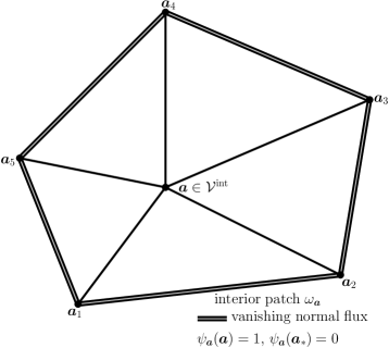
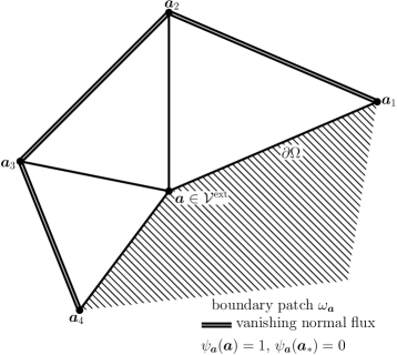
Figure 1: Patches ${\mathcal{T}_{{\bm{a}}}}$, vanishing normal flux conditions in the local Raviart–Thomas–Nédélec spaces $\bm{V}_{\mathcal{T}}^{\bm{a}}$, and hat functions $\psi_{{\bm{a}}}$: interior (left) and boundary (right) vertex ${\bm{a}}\in\mathcal{V}$

Recall that $u_{{\mathcal{T}}}\in V_{{\mathcal{T}}}$ with $V_{{\mathcal{T}}}={\mathbb{P}}_{p}(\mathcal{T})\cap H^{1}_{0}(\Omega)$ is the finite element solution given by (1.5). Let $C_{*}$ be the constant composed of the constants of the trace and inverse inequalities and given by (2.7). Our construction is:

Definition 2.3 (Flux $\bm{\sigma}_{{\mathcal{T}}}$ and potential $\phi_{{\mathcal{T}}}$).

For each vertex ${\bm{a}}\in\mathcal{V}$, let $(\bm{\sigma}_{{\mathcal{T}}}^{{\bm{a}}},\phi_{{\mathcal{T}}}^{{\bm{a}}})\in\bm{V}_{\mathcal{T}}^{\bm{a}}\times Q_{\mathcal{T}}^{{\bm{a}}}$ be defined by the local constrained minimization problem

$$(\bm{\sigma}_{{\mathcal{T}}}^{{\bm{a}}},\phi_{{\mathcal{T}}}^{{\bm{a}}})\coloneqq\operatorname*{arg\,min}_{\begin{subarray}{c}(\bm{v}_{{\mathcal{T}}},q_{\mathcal{T}})\in\bm{V}_{\mathcal{T}}^{\bm{a}}\times Q_{\mathcal{T}}^{{\bm{a}}}\\ \nabla{\cdot}\bm{v}_{{\mathcal{T}}}+\kappa^{2}q_{\mathcal{T}}=\Pi_{{\mathcal{T}}}(f\psi_{{\bm{a}}})-\varepsilon^{2}\nabla u_{{\mathcal{T}}}{\cdot}\nabla\psi_{{\bm{a}}}\end{subarray}}w_{{\bm{a}}}^{2}\lVert\varepsilon\psi_{{\bm{a}}}\nabla u_{{\mathcal{T}}}+\varepsilon^{-1}\bm{v}_{{\mathcal{T}}}\rVert_{{\omega_{\bm{a}}}}^{2}+\lVert\kappa\left[\Pi_{{\mathcal{T}}}(\psi_{{\bm{a}}}u_{{\mathcal{T}}})-q_{\mathcal{T}}\right]\rVert^{2}_{{\omega_{\bm{a}}}}$$ (2.9a)

with the weight

$$w_{{\bm{a}}}\coloneqq\min\left\{1,C_{*}\sqrt{\frac{\varepsilon}{\kappa h_{{\omega_{\bm{a}}}}}}\right\}.$$ (2.9b)

Then, extending each $$\bm{\sigma}_{{\mathcal{T}}}^{{\bm{a}}} \phi_{{\mathcal{T}}}^{{\bm{a}}} {\omega_{\bm{a}}} \bm{\sigma}_{{\mathcal{T}}}\in\bm{RTN}_{p}(\mathcal{T}) \phi_{{\mathcal{T}}}\in{\mathbb{P}}_{p}(\mathcal{T})$$ and by zero outside of the patch , and are given by

$$\bm{\sigma}_{{\mathcal{T}}}\coloneqq\sum_{{\bm{a}}\in\mathcal{V}}\bm{\sigma}_{{\mathcal{T}}}^{{\bm{a}}},\quad\phi_{{\mathcal{T}}}\coloneqq\sum_{{\bm{a}}\in\mathcal{V}}\phi_{{\mathcal{T}}}^{{\bm{a}}}.$$ (2.9c)

We remark that for an interior vertex ${\bm{a}}\in\mathcal{V}^{\mathrm{int}}$, we have

$$(\Pi_{{\mathcal{T}}}(f\psi_{{\bm{a}}})-\varepsilon^{2}\nabla u_{{\mathcal{T}}}{\cdot}\nabla\psi_{{\bm{a}}},1)_{{\omega_{\bm{a}}}}=(f,\psi_{{\bm{a}}})_{\omega_{\bm{a}}}-\varepsilon^{2}(\nabla u_{{\mathcal{T}}},\nabla\psi_{{\bm{a}}})_{{\omega_{\bm{a}}}}=\kappa^{2}(u_{{\mathcal{T}}},\psi_{{\bm{a}}})_{{\omega_{\bm{a}}}}$$ (2.10)

by Galerkin orthogonality with $\psi_{{\bm{a}}}\in V_{{\mathcal{T}}}$ as a test function in (1.5). Since

$$(\nabla{\cdot}\bm{\sigma}_{{\mathcal{T}}}^{{\bm{a}}},1)_{\omega_{\bm{a}}}=(\bm{\sigma}_{{\mathcal{T}}}^{{\bm{a}}}{\cdot}{\bm{n}}_{\omega_{\bm{a}}},1)_{\partial{\omega_{\bm{a}}}}=0$$

by Green’s theorem and the vanishing normal flux condition imposed in the definition (2.8a) of $\bm{V}_{\mathcal{T}}^{\bm{a}}$, it follows that $\phi_{{\mathcal{T}}}^{{\bm{a}}}$ necessarily satisfies the mean-value property

$$(\phi_{{\mathcal{T}}}^{{\bm{a}}},1)_{{\omega_{\bm{a}}}}=(\psi_{{\bm{a}}}u_{{\mathcal{T}}},1)_{{\omega_{\bm{a}}}}\qquad\forall{\bm{a}}\in\mathcal{V}^{\mathrm{int}},$$

whenever $\kappa>0$. If $\kappa=0$ instead, then $\phi_{{\mathcal{T}}}^{{\bm{a}}}$ is undefined by (2.9a) but one remarks that it is no longer needed anywhere in the paper. In this case, Definition 2.3 coincides with [7, equation (9)], [18, Definition 6.9], or [19, Construction 3.4]; in particular, the Neumann compatibility condition of problem (2.9a) for ${\bm{a}}\in\mathcal{V}^{\mathrm{int}}$ follows from (2.10).

In practice, the constrained minimization problem (2.9a) is solved through its Euler–Lagrange equations, which can be reduced to solving a linear system of dimension $\operatorname{dim}\bm{V}_{\mathcal{T}}^{\bm{a}}+\operatorname{dim}Q_{\mathcal{T}}^{{\bm{a}}}$ in the present context. This problem reads: find $(\bm{\sigma}_{{\mathcal{T}}}^{{\bm{a}}},\phi_{{\mathcal{T}}}^{{\bm{a}}})\in\bm{V}_{\mathcal{T}}^{\bm{a}}\times Q_{\mathcal{T}}^{{\bm{a}}}$ with $\phi_{{\mathcal{T}}}^{{\bm{a}}}=\gamma_{\mathcal{T}}^{{\bm{a}}}+\Pi_{{\mathcal{T}}}(\psi_{{\bm{a}}}u_{{\mathcal{T}}})$ and $(\bm{\sigma}_{{\mathcal{T}}}^{{\bm{a}}},\gamma_{\mathcal{T}}^{{\bm{a}}})\in\bm{V}_{\mathcal{T}}^{\bm{a}}\times Q_{\mathcal{T}}^{{\bm{a}}}$ such that

$$\varepsilon^{-2}w_{{\bm{a}}}^{2}(\bm{\sigma}_{{\mathcal{T}}}^{{\bm{a}}},\bm{v}_{\mathcal{T}})_{\omega_{\bm{a}}}-(\gamma_{\mathcal{T}}^{{\bm{a}}},\nabla{\cdot}\bm{v}_{\mathcal{T}})_{\omega_{\bm{a}}} =-w_{{\bm{a}}}^{2}(\psi_{{\bm{a}}}\nabla u_{{\mathcal{T}}},\bm{v}_{\mathcal{T}})_{\omega_{\bm{a}}} \forall\bm{v}_{\mathcal{T}}\in\bm{V}_{\mathcal{T}}^{\bm{a}},$$ (2.11a)

$$(\nabla{\cdot}\bm{\sigma}_{{\mathcal{T}}}^{{\bm{a}}},q_{\mathcal{T}})_{\omega_{\bm{a}}}+\kappa^{2}(\gamma_{\mathcal{T}}^{{\bm{a}}},q_{\mathcal{T}})_{\omega_{\bm{a}}} =(f\psi_{{\bm{a}}}-\kappa^{2}\psi_{{\bm{a}}}u_{{\mathcal{T}}}-\varepsilon^{2}\nabla u_{{\mathcal{T}}}{\cdot}\nabla\psi_{{\bm{a}}},q_{\mathcal{T}})_{\omega_{\bm{a}}} \forall q_{\mathcal{T}}\in Q_{\mathcal{T}}^{{\bm{a}}}.$$ (2.11b)

2.4 Properties of $\bm{\sigma}_{{\mathcal{T}}}$ and $\phi_{{\mathcal{T}}}$

We have constructed $\bm{\sigma}_{{\mathcal{T}}}$ and $\phi_{{\mathcal{T}}}$ such that the following holds:

Proposition 2.4 ($\bm{H}(\mathrm{div},\Omega)$-conformity of $\bm{\sigma}_{{\mathcal{T}}}$, equilibration).

Let $\bm{\sigma}_{{\mathcal{T}}}\in\bm{RTN}_{p}(\mathcal{T})$ and $\phi_{{\mathcal{T}}}\in{\mathbb{P}}_{p}(\mathcal{T})$ be given by Definition 2.3. Then $\bm{\sigma}_{{\mathcal{T}}}$ belongs to $\bm{H}(\mathrm{div},\Omega)$, and $\bm{\sigma}_{{\mathcal{T}}}$ and $\phi_{{\mathcal{T}}}$ satisfy the equilibration property (1.10).

Proof.

First, the $\bm{H}(\mathrm{div},\Omega)$-conformity of $\bm{\sigma}_{{\mathcal{T}}}$ follows from the fact that, for any vertex ${\bm{a}}\in\mathcal{V}$, the zero extension of $\bm{\sigma}_{{\mathcal{T}}}^{{\bm{a}}}$ belongs to $\bm{H}(\mathrm{div},\Omega)$ as a result of the vanishing normal flux boundary conditions in the space $\bm{V}_{\mathcal{T}}^{\bm{a}}$. Then, to show (1.10), we employ the constraint in (2.9a) together with (2.9c):

$$\nabla{\cdot}\bm{\sigma}_{{\mathcal{T}}}+\kappa^{2}\phi_{{\mathcal{T}}}=\sum_{{\bm{a}}\in\mathcal{V}}[\nabla{\cdot}\bm{\sigma}_{{\mathcal{T}}}^{{\bm{a}}}+\kappa^{2}\phi_{{\mathcal{T}}}^{{\bm{a}}}]=\sum_{{\bm{a}}\in\mathcal{V}}\big{[}\Pi_{{\mathcal{T}}}(f\psi_{{\bm{a}}})-\varepsilon^{2}\nabla u_{{\mathcal{T}}}{\cdot}\nabla\psi_{{\bm{a}}}\big{]}=\Pi_{{\mathcal{T}}}f,$$

where we have used the fact that the hat functions $\{\psi_{{\bm{a}}}\}_{{\bm{a}}\in\mathcal{V}}$ form a partition of unity over $\Omega$, i.e. $\sum_{{\bm{a}}\in\mathcal{V}}\psi_{{\bm{a}}}=1$. ∎

3 A computable guaranteed a posteriori error estimate

This section presents our guaranteed and fully computable a posteriori error estimate. The following upper bound on the energy norm of the error builds on [9, Theorems 3.1 and 4.4] and [5, Lemma 2]. It employs additionally the concept of a potential reconstruction $\phi_{{\mathcal{T}}}$ that will turn out crucial for a simple and robust flux equilibration. Moreover, it relies on the trace and inverse inequalities of Section 2.2 to make appear the crucial weighs (cut-off factors), with the constant $C_{*}$ given by (2.7).

Theorem 3.1 (Guaranteed a posteriori error estimate).

Let $u$ be the weak solution of problem (1.1) given by (1.3) and let $u_{{\mathcal{T}}}\in V_{{\mathcal{T}}}$ be its finite element approximation given by (1.5). Let $\bm{\sigma}_{{\mathcal{T}}}\in\bm{RTN}_{p}(\mathcal{T})\cap\bm{H}(\mathrm{div},\Omega)$ and $\phi_{{\mathcal{T}}}\in{\mathbb{P}}_{p}(\mathcal{T})$ be given by Definition 2.3. Then the following upper bound for the energy norm of the error holds:

$${\lvert\kern-1.07639pt\lvert\kern-1.07639pt\lvert u-u_{{\mathcal{T}}}\rvert\kern-1.07639pt\rvert\kern-1.07639pt\rvert}^{2}\leq\sum_{{K}\in\mathcal{T}}\left[w_{{K}}\lVert\varepsilon\nabla u_{{\mathcal{T}}}+\varepsilon^{-1}\bm{\sigma}_{{\mathcal{T}}}\rVert_{K}+\lVert\kappa\left(u_{{\mathcal{T}}}-\phi_{{\mathcal{T}}}\right)\rVert_{K}+\widetilde{w}_{{K}}\lVert f-\Pi_{{\mathcal{T}}}f\rVert_{K}\right]^{2},$$ (3.1)

where the weights $w_{{K}}$ and $\widetilde{w}_{{K}}$ are respectively defined by

$$w_{{K}}\coloneqq\min\left\{1,C_{*}\sqrt{\frac{\varepsilon}{\kappa h_{{K}}}}\right\},\quad\widetilde{w}_{{K}}\coloneqq\min\left\{\frac{h_{{K}}}{\pi\varepsilon},\frac{1}{\kappa}\right\},\qquad{K}\in\mathcal{T}.$$ (3.2)

Proof.

First, we note that the energy norm of the error ${\lvert\kern-1.07639pt\lvert\kern-1.07639pt\lvert u-u_{{\mathcal{T}}}\rvert\kern-1.07639pt\rvert\kern-1.07639pt\rvert}$ is related to the residual $\mathcal{R}(u_{{\mathcal{T}}})\in H^{-1}(\Omega)$, defined by

$$\langle\mathcal{R}(u_{{\mathcal{T}}}),v\rangle\coloneqq(f,v)-a(u_{{\mathcal{T}}},v),\qquad v\in H^{1}_{0}(\Omega),$$

through the identity

$${\lvert\kern-1.07639pt\lvert\kern-1.07639pt\lvert u-u_{{\mathcal{T}}}\rvert\kern-1.07639pt\rvert\kern-1.07639pt\rvert}={\lvert\kern-1.07639pt\lvert\kern-1.07639pt\lvert R(u_{{\mathcal{T}}})\rvert\kern-1.07639pt\rvert\kern-1.07639pt\rvert}_{*},\quad{\lvert\kern-1.07639pt\lvert\kern-1.07639pt\lvert R(u_{{\mathcal{T}}})\rvert\kern-1.07639pt\rvert\kern-1.07639pt\rvert}_{*}\coloneqq\sup_{v\in H^{1}_{0}(\Omega),\,{\lvert\kern-0.75346pt\lvert\kern-0.75346pt\lvert v\rvert\kern-0.75346pt\rvert\kern-0.75346pt\rvert}=1}\langle\mathcal{R}(u_{{\mathcal{T}}}),v\rangle,$$ (3.3)

cf., e.g., [35, equation (4.1)]. Consider now $\langle\mathcal{R}(u_{{\mathcal{T}}}),v\rangle$ for a fixed function $v\in H^{1}_{0}(\Omega)$. Since $\bm{\sigma}_{{\mathcal{T}}}\in\bm{H}(\mathrm{div},\Omega)$ and $v\in H^{1}_{0}(\Omega)$, Green’s theorem gives $(\bm{\sigma}_{{\mathcal{T}}},\nabla v)+(\nabla{\cdot}\bm{\sigma}_{{\mathcal{T}}},v)=0$, so

$$\langle\mathcal{R}(u_{{\mathcal{T}}}),v\rangle=(f,v)-a(u_{{\mathcal{T}}},v)=(f-\Pi_{{\mathcal{T}}}f,v)+(\kappa(\phi_{{\mathcal{T}}}-u_{{\mathcal{T}}}),\kappa v)-(\varepsilon\nabla u_{{\mathcal{T}}}+\varepsilon^{-1}\bm{\sigma}_{{\mathcal{T}}},\varepsilon\nabla v),$$ (3.4)

where we have also used the equilibration identity (1.10). We now proceed by estimating each term in (3.4) elementwise.

For each element ${K}\in\mathcal{T}$, we use the identity $(f-\Pi_{{\mathcal{T}}}f,v)_{K}=(f-\Pi_{{\mathcal{T}}}f,v-\Pi_{{\mathcal{T}}}v)_{K}$ and the Poincaré–Friedrichs inequality on the convex element ${K}$, i.e. $\lVert v-\Pi_{{\mathcal{T}}}v\rVert_{K}\leq\frac{h_{K}}{\pi}\lVert\nabla v\rVert_{K}$ for any $v\in H^{1}({K})$, together with the energy error definition (1.13), to obtain the following bound

$$\lvert(f-\Pi_{{\mathcal{T}}}f,v)_{K}\rvert\leq\lVert f-\Pi_{\mathcal{T}}f\rVert_{K}\min\left\{\frac{h_{K}}{\pi\varepsilon}\lVert\varepsilon\nabla v\rVert_{K},\frac{1}{\kappa}\lVert\kappa v\rVert_{K}\right\}\leq\widetilde{w}_{{K}}\lVert f-\Pi_{\mathcal{T}}f\rVert_{K}{\lvert\kern-1.07639pt\lvert\kern-1.07639pt\lvert v\rvert\kern-1.07639pt\rvert\kern-1.07639pt\rvert}_{K}.$$ (3.5)

Here, actually, a little sharper bound is possible by a convex combination of the two possibilities, but we prefer to use the simple form (3.5) with $\widetilde{w}_{{K}}$ in the form of minimum given by (3.2).

Next, it is clear that

$$\lvert(\varepsilon\nabla u_{{\mathcal{T}}}+\varepsilon^{-1}\bm{\sigma}_{{\mathcal{T}}},\varepsilon\nabla v)_{{K}}\rvert\leq\lVert\varepsilon\nabla u_{{\mathcal{T}}}+\varepsilon^{-1}\bm{\sigma}_{{\mathcal{T}}}\rVert_{K}{\lvert\kern-1.07639pt\lvert\kern-1.07639pt\lvert v\rvert\kern-1.07639pt\rvert\kern-1.07639pt\rvert}_{K}$$ (3.6)

for each ${K}\in\mathcal{T}$. However, this is not necessarily the sharpest possible estimate in the singularly perturbed regime $\kappa\gg\varepsilon$. Therefore, following the idea of [9, Proof of Theorem 4.4], we use Green’s theorem elementwise together with the fact that $\nabla v=\nabla(v-\overline{v}_{{K}})$, where $\overline{v}_{{K}}$ denotes the mean-value of $v$ on ${K}$. This gives

$$(\varepsilon\nabla u_{{\mathcal{T}}}+\varepsilon^{-1}\bm{\sigma}_{{\mathcal{T}}},\varepsilon\nabla v)_{{K}}=((\varepsilon\nabla u_{{\mathcal{T}}}+\varepsilon^{-1}\bm{\sigma}_{{\mathcal{T}}}){\cdot}\bm{n},\varepsilon(v-\overline{v}_{{K}}))_{\partial{K}}-(\nabla{\cdot}\left(\varepsilon\nabla u_{{\mathcal{T}}}+\varepsilon^{-1}\bm{\sigma}_{{\mathcal{T}}}\right),\varepsilon(v-\overline{v}_{{K}}))_{{K}}.$$

The $L^{2}({K})$-stability of the mean-value, $\lVert v-\overline{v}_{{K}}\rVert_{K}\leq\lVert v\rVert_{K}$, Young’s inequality

$$\lVert\varepsilon\nabla v\rVert_{{K}}^{\frac{1}{2}}\lVert\kappa v\rVert^{\frac{1}{2}}_{K}\leq\frac{1}{\sqrt{2}}{\lvert\kern-1.07639pt\lvert\kern-1.07639pt\lvert v\rvert\kern-1.07639pt\rvert\kern-1.07639pt\rvert}_{{K}},$$ (3.7)

and the multiplicative trace inequality (2.3) altogether lead to

$$\varepsilon\lVert v-\overline{v}_{{K}}\rVert_{\partial{K}}\leq C_{\mathrm{Tr}}\varepsilon^{{\frac{1}{2}}}\lVert\varepsilon\nabla v\rVert_{{K}}^{\frac{1}{2}}\lVert v\rVert_{{K}}^{\frac{1}{2}}\leq\frac{C_{\mathrm{Tr}}}{\sqrt{2}}\sqrt{h_{K}}\sqrt{\frac{\varepsilon}{\kappa h_{{K}}}}{\lvert\kern-1.07639pt\lvert\kern-1.07639pt\lvert v\rvert\kern-1.07639pt\rvert\kern-1.07639pt\rvert}_{{K}}.$$

Combined with the inverse inequality (2.4), we find that

$$\lvert((\varepsilon\nabla u_{{\mathcal{T}}}+\varepsilon^{-1}\bm{\sigma}_{{\mathcal{T}}}){\cdot}\bm{n},\varepsilon(v-\overline{v}_{{K}}))_{\partial{K}}\rvert\leq\frac{C_{p+1,d,\partial K}C_{\mathrm{Tr}}}{\sqrt{2}}\sqrt{\frac{\varepsilon}{\kappa h_{{K}}}}\lVert\varepsilon\nabla u_{{\mathcal{T}}}+\varepsilon^{-1}\bm{\sigma}_{{\mathcal{T}}}\rVert_{{K}}{\lvert\kern-1.07639pt\lvert\kern-1.07639pt\lvert v\rvert\kern-1.07639pt\rvert\kern-1.07639pt\rvert}_{K}.$$ (3.8)

The $L^{2}({K})$-stability of the mean-value, the Poincaré–Friedrichs inequality in the form $\lVert v-\overline{v}_{{K}}\rVert_{K}\leq\frac{h_{K}}{\pi}\lVert\nabla v\rVert_{K}$, and (3.7) yield

$$\varepsilon\lVert v-\overline{v}_{{K}}\rVert_{{K}}\leq\varepsilon\lVert v\rVert_{{K}}^{\frac{1}{2}}h_{K}^{\frac{1}{2}}\pi^{-\frac{1}{2}}\lVert\nabla v\rVert_{K}^{\frac{1}{2}}\leq\frac{h_{K}}{\sqrt{2\pi}}\sqrt{\frac{\varepsilon}{\kappa h_{{K}}}}{\lvert\kern-1.07639pt\lvert\kern-1.07639pt\lvert v\rvert\kern-1.07639pt\rvert\kern-1.07639pt\rvert}_{{K}}.$$

Thus, combined with the inverse inequality (2.4), we find that

$$\lvert(\nabla{\cdot}\left(\varepsilon\nabla u_{{\mathcal{T}}}+\varepsilon^{-1}\bm{\sigma}_{{\mathcal{T}}}\right),\varepsilon(v-\overline{v}_{{K}}))_{{K}}\rvert\leq\frac{1}{\sqrt{2}}\frac{1}{\sqrt{\pi}}C_{p+1,d,K}\sqrt{\frac{\varepsilon}{\kappa h_{{K}}}}\lVert\varepsilon\nabla u_{{\mathcal{T}}}+\varepsilon^{-1}\bm{\sigma}_{{\mathcal{T}}}\rVert_{{K}}{\lvert\kern-1.07639pt\lvert\kern-1.07639pt\lvert v\rvert\kern-1.07639pt\rvert\kern-1.07639pt\rvert}_{{K}}.$$ (3.9)

Therefore, combining inequalities (3.6), (3.8), and (3.9), we get

$$\lvert(\varepsilon\nabla u_{{\mathcal{T}}}+\varepsilon^{-1}\bm{\sigma}_{{\mathcal{T}}},\varepsilon\nabla v)_{{K}}\rvert\leq w_{{K}}\lVert\varepsilon\nabla u_{{\mathcal{T}}}+\varepsilon^{-1}\bm{\sigma}_{{\mathcal{T}}}\rVert_{{K}}{\lvert\kern-1.07639pt\lvert\kern-1.07639pt\lvert v\rvert\kern-1.07639pt\rvert\kern-1.07639pt\rvert}_{{K}}\quad\forall{K}\in\mathcal{T}$$ (3.10)

with $w_{{K}}$ given by (3.2) and $C_{*}$ given in (2.7). As a side remark, it is possible to obtain a slightly sharper, at the expense of making the weight $w_{{K}}$ more complicated than the simple form given by (3.2).

Finally, we can apply the Cauchy–Schwarz inequality to see that $|(\kappa(\phi_{{\mathcal{T}}}-u_{{\mathcal{T}}}),\kappa v)_{{K}}|\leq\lVert\kappa\left(u_{{\mathcal{T}}}-\phi_{{\mathcal{T}}}\right)\rVert_{{K}}{\lvert\kern-1.07639pt\lvert\kern-1.07639pt\lvert v\rvert\kern-1.07639pt\rvert\kern-1.07639pt\rvert}_{{K}}$. Therefore, we deduce from (3.4) and the above inequalities that

$$\lvert\langle\mathcal{R}(u_{{\mathcal{T}}}),v\rangle\rvert\leq\sum_{{K}\in\mathcal{T}}\left[w_{{K}}\lVert\varepsilon\nabla u_{{\mathcal{T}}}+\varepsilon^{-1}\bm{\sigma}_{{\mathcal{T}}}\rVert_{{K}}+\lVert\kappa\left(u_{{\mathcal{T}}}-\phi_{{\mathcal{T}}}\right)\rVert_{{K}}+\widetilde{w}_{{K}}\lVert f-\Pi_{{\mathcal{T}}}f\rVert_{{K}}\right]{\lvert\kern-1.07639pt\lvert\kern-1.07639pt\lvert v\rvert\kern-1.07639pt\rvert\kern-1.07639pt\rvert}_{{K}},$$

which implies the upper bound on the error (3.1) after another Cauchy–Schwarz inequality, using (3.3) and $\sum_{{K}\in\mathcal{T}}{\lvert\kern-1.07639pt\lvert\kern-1.07639pt\lvert v\rvert\kern-1.07639pt\rvert\kern-1.07639pt\rvert}_{K}^{2}={\lvert\kern-1.07639pt\lvert\kern-1.07639pt\lvert v\rvert\kern-1.07639pt\rvert\kern-1.07639pt\rvert}^{2}$. ∎

4 Efficiency and robustness of the estimate

This section establishes the local (and consequently global) efficiency and robustness of our a posteriori error estimate.

4.1 A basic stability result

The main tool in the analysis of efficiency is the following stability result, where, we recall, the broken and the patchwise ${\bm{H}}(\mathrm{div})$-conforming Raviart–Thomas–Nédélec spaces $\bm{RTN}_{p}({\mathcal{T}_{{\bm{a}}}})$ and $\bm{V}_{\mathcal{T}}^{\bm{a}}$ are respectively given by (2.2) and (2.8).

Lemma 4.1 (Stability of patchwise flux equilibration).

Let a vertex ${\bm{a}}\in\mathcal{V}$ be fixed, and let $g_{{\mathcal{T}}}\in{\mathbb{P}}_{p}({\mathcal{T}_{{\bm{a}}}})$ and $\bm{\tau}_{{\mathcal{T}}}\in\bm{RTN}_{p}({\mathcal{T}_{{\bm{a}}}})$ be given discontinuous piecewise polynomial functions, with the Neumann compatibility condition $(g_{{\mathcal{T}}},1)_{{\omega_{\bm{a}}}}=0$ satisfied if ${\bm{a}}\in\mathcal{V}^{\mathrm{int}}$. Then, there holds

$$\min_{\begin{subarray}{c}\bm{v}_{{\mathcal{T}}}\in\bm{V}_{\mathcal{T}}^{\bm{a}}\\ \nabla{\cdot}\bm{v}_{{\mathcal{T}}}=g_{{\mathcal{T}}}\end{subarray}}\lVert\bm{\tau}_{{\mathcal{T}}}+\bm{v}_{{\mathcal{T}}}\rVert_{{\omega_{\bm{a}}}}\lesssim\sup_{\begin{subarray}{c}v\in H^{1}_{*}({\omega_{\bm{a}}})\\ \lVert\nabla v\rVert_{{\omega_{\bm{a}}}}=1\end{subarray}}\big{\{}(g_{{\mathcal{T}}},v)_{{\omega_{\bm{a}}}}-(\bm{\tau}_{{\mathcal{T}}},\nabla v)_{{\omega_{\bm{a}}}}\big{\}},$$ (4.1)

where $H^{1}_{*}({\omega_{\bm{a}}})$ is the subspace of functions in $H^{1}({\omega_{\bm{a}}})$ that have mean-value zero on the patch subdomain ${\omega_{\bm{a}}}$ if ${\bm{a}}\in\mathcal{V}^{\mathrm{int}}$ is an interior vertex, or that vanish on $\partial{\omega_{\bm{a}}}\cap\partial\Omega$ if ${\bm{a}}\in\mathcal{V}^{\mathrm{ext}}$ is a boundary vertex.

The above result holds for any dimension $d\geq 1$, although some additional properties are known for $d\leq 3$. Indeed, in the case where $d=2$, it is shown in [7, Theorem 7] that the constant in (4.1) is in fact independent of the polynomial degree $p$, i.e. $p$-robust. The extension of the $p$-robustness of the bound to the case of $d=3$ was shown in [20, Corollaries 3.3 and 3.6]. It is also possible to extend similar results of this kind to situations with hanging nodes and locally refined submeshes, as shown in [17].

4.2 Stability with respect to residual estimators

The next lemma shows that the local contributions of the equilibrated flux a posteriori estimators of Definition 2.3 lie below the local residual estimators as defined in (1.7), with the element residuals $r_{\mathcal{T}}$ and face residuals $j_{\mathcal{T}}$ are defined by (1.8) and the weights $\alpha_{{K}}$ and $\alpha_{F}$ defined by (1.9).

Lemma 4.2 (Stability of patchwise flux equilibration with respect to residual estimators).

For each ${\bm{a}}\in\mathcal{V}$, let $\bm{\sigma}_{{\mathcal{T}}}^{{\bm{a}}}$ and $\phi_{{\mathcal{T}}}^{{\bm{a}}}$ be defined by (2.9a). Then

$$w_{{\bm{a}}}^{2}\lVert\varepsilon\psi_{{\bm{a}}}\nabla u_{{\mathcal{T}}}+\varepsilon^{-1}\bm{\sigma}_{{\mathcal{T}}}^{{\bm{a}}}\rVert_{{\omega_{\bm{a}}}}^{2}+\lVert\kappa\left[\Pi_{{\mathcal{T}}}(\psi_{{\bm{a}}}u_{{\mathcal{T}}})-\phi_{{\mathcal{T}}}^{{\bm{a}}}\right]\rVert_{{\omega_{\bm{a}}}}^{2}\lesssim\sum_{{K}\in{\mathcal{T}_{{\bm{a}}}}}\alpha_{{K}}^{2}\lVert r_{\mathcal{T}}\rVert_{{K}}^{2}+\sum_{F\in\mathcal{F}_{{\bm{a}}}}\varepsilon^{-1}\alpha_{F}\lVert j_{\mathcal{T}}\rVert_{F}^{2}.$$ (4.2)

Proof.

Let a vertex ${\bm{a}}\in\mathcal{V}$ be fixed. Since $\bm{\sigma}_{{\mathcal{T}}}^{{\bm{a}}}$ and $\phi_{{\mathcal{T}}}^{{\bm{a}}}$ are defined as minimizers of the functional in the right-hand side of (2.9a), it is enough to prove that there always exists some $\bm{v}_{{\mathcal{T}}}^{*}\in\bm{V}_{\mathcal{T}}^{\bm{a}}$ and $q_{\mathcal{T}}^{*}\in Q_{\mathcal{T}}^{{\bm{a}}}$ that satisfy the constraint $\nabla{\cdot}\bm{v}_{{\mathcal{T}}}^{*}+\kappa^{2}q_{\mathcal{T}}^{*}=\Pi_{{\mathcal{T}}}(f\psi_{{\bm{a}}})-\varepsilon^{2}\nabla u_{{\mathcal{T}}}{\cdot}\nabla\psi_{{\bm{a}}}$ and that satisfy the bound (4.2) with $\bm{v}_{{\mathcal{T}}}^{*}$ in place of $\bm{\sigma}_{{\mathcal{T}}}^{{\bm{a}}}$ and $q_{\mathcal{T}}^{*}$ in place of $\phi_{{\mathcal{T}}}^{{\bm{a}}}$. The specific construction depends on the mesh size and the problem parameters $\varepsilon$ and $\kappa$, as we now show.

Case 1, $\varepsilon/h_{{\omega_{\bm{a}}}}\leq\kappa$ (reaction dominance). Up to a constant, we have $\kappa^{-1}\lesssim h_{{K}}/\varepsilon$ and $\kappa^{-1}\lesssim h_{F}/\varepsilon$ for all elements ${K}\in{\mathcal{T}_{{\bm{a}}}}$ and all interior faces $F\in\mathcal{F}_{{\bm{a}}}$. In this case, we adopt the following construction. Let

$$\rho_{{\bm{a}}}\coloneqq\frac{1}{\lvert{\omega_{\bm{a}}}\rvert}(\psi_{{\bm{a}}}r_{\mathcal{T}},1)_{{\omega_{\bm{a}}}}=\frac{1}{\lvert{\omega_{\bm{a}}}\rvert}(\psi_{{\bm{a}}}(f+\varepsilon^{2}\Delta_{\mathcal{T}}u_{{\mathcal{T}}}-\kappa^{2}u_{{\mathcal{T}}}),1)_{\omega_{\bm{a}}},\qquad{\bm{a}}\in\mathcal{V}^{\mathrm{int}},$$

and $\rho_{{\bm{a}}}\coloneqq 0$ otherwise. Next, we define

$$q_{\mathcal{T}}^{*}\coloneqq\frac{1}{\kappa^{2}}\left(\Pi_{{\mathcal{T}}}\left(f\psi_{{\bm{a}}}\right)+\varepsilon^{2}\psi_{{\bm{a}}}\Delta_{\mathcal{T}}u_{{\mathcal{T}}}-\rho_{{\bm{a}}}\right),\quad\bm{v}_{{\mathcal{T}}}^{*}\coloneqq\operatorname*{arg\,min}_{\begin{subarray}{c}\bm{v}_{{\mathcal{T}}}\in\bm{V}_{\mathcal{T}}^{\bm{a}}\\ \nabla{\cdot}\bm{v}_{{\mathcal{T}}}=g_{{\mathcal{T}}}^{*}\end{subarray}}\lVert\varepsilon^{2}\psi_{{\bm{a}}}\nabla u_{{\mathcal{T}}}+\bm{v}_{{\mathcal{T}}}\rVert_{{\omega_{\bm{a}}}},$$ (4.3)

where

$$g_{{\mathcal{T}}}^{*}\coloneqq-\varepsilon^{2}(\nabla u_{{\mathcal{T}}}{\cdot}\nabla\psi_{{\bm{a}}}+\psi_{{\bm{a}}}\Delta_{\mathcal{T}}u_{{\mathcal{T}}})+\rho_{{\bm{a}}}.$$

It is easy to check that if ${\bm{a}}\in\mathcal{V}^{\mathrm{int}}$, then $(g_{{\mathcal{T}}}^{*},1)_{{\omega_{\bm{a}}}}=0$, since the Galerkin orthogonality (take $v_{{\mathcal{T}}}=\psi_{{\bm{a}}}$ in (1.5)) implies that

$$(g_{{\mathcal{T}}}^{*},1)_{{\omega_{\bm{a}}}}=(f,\psi_{{\bm{a}}})-\varepsilon^{2}(\nabla u_{{\mathcal{T}}},\nabla\psi_{{\bm{a}}})-\kappa^{2}(u_{{\mathcal{T}}},\psi_{{\bm{a}}})=0.$$ (4.4)

Therefore, it follows that $q_{\mathcal{T}}^{*}\in Q_{\mathcal{T}}^{{\bm{a}}}$ and $\bm{v}_{{\mathcal{T}}}^{*}\in\bm{V}_{\mathcal{T}}^{\bm{a}}$ are well-defined and that they satisfy the constraint $\nabla{\cdot}\bm{v}_{{\mathcal{T}}}^{*}+\kappa^{2}q_{\mathcal{T}}^{*}=\Pi_{{\mathcal{T}}}(f\psi_{{\bm{a}}})-\varepsilon^{2}\nabla u_{{\mathcal{T}}}{\cdot}\nabla\psi_{{\bm{a}}}$.

We now bound $w_{{\bm{a}}}^{2}\lVert\varepsilon^{2}\psi_{{\bm{a}}}\nabla u_{{\mathcal{T}}}+\bm{v}_{{\mathcal{T}}}^{*}\rVert_{{\omega_{\bm{a}}}}^{2}$ and $\lVert\kappa\left[\Pi_{{\mathcal{T}}}(\psi_{{\bm{a}}}u_{{\mathcal{T}}})-q_{\mathcal{T}}^{*}\right]\rVert_{{\omega_{\bm{a}}}}^{2}$. First, we obtain

$$\lVert\kappa\left[\Pi_{{\mathcal{T}}}(\psi_{{\bm{a}}}u_{{\mathcal{T}}})-q_{\mathcal{T}}^{*}\right]\rVert_{{\omega_{\bm{a}}}}^{2}=\frac{1}{\kappa^{2}}\lVert\Pi_{{\mathcal{T}}}(\psi_{{\bm{a}}}r_{\mathcal{T}})-\rho_{{\bm{a}}}\rVert_{{\omega_{\bm{a}}}}^{2}\leq\frac{1}{\kappa^{2}}\lVert r_{\mathcal{T}}\rVert_{{\omega_{\bm{a}}}}^{2}\lesssim\sum_{{K}\in{\mathcal{T}_{{\bm{a}}}}}\alpha_{{K}}^{2}\lVert r_{\mathcal{T}}\rVert_{{K}}^{2},$$

where we have used the stability of the $L^{2}$-projection (note that $\rho_{{\bm{a}}}$ is also the mean value of $\Pi_{{\mathcal{T}}}(\psi_{{\bm{a}}}r_{\mathcal{T}})$ on ${\omega_{\bm{a}}}$ for ${\bm{a}}\in\mathcal{V}^{\mathrm{int}}$) and the fact that $\lVert\psi_{{\bm{a}}}\rVert_{\infty,{\omega_{\bm{a}}}}=1$ to bound $\lVert\Pi_{{\mathcal{T}}}(\psi_{{\bm{a}}}r_{\mathcal{T}})-\rho_{{\bm{a}}}\rVert_{{\omega_{\bm{a}}}}$. Next, we apply Lemma 4.1 to bound $w_{{\bm{a}}}^{2}\lVert\varepsilon^{2}\psi_{{\bm{a}}}\nabla u_{{\mathcal{T}}}+\bm{v}_{{\mathcal{T}}}^{*}\rVert_{{\omega_{\bm{a}}}}^{2}$. Note first that for an interior vertex ${\bm{a}}\in\mathcal{V}^{\mathrm{int}}$, $(\rho_{{\bm{a}}},v)_{{\omega_{\bm{a}}}}=0$ since $v\in H^{1}_{*}({\omega_{\bm{a}}})$ implies that $v$ is orthogonal to constant functions on ${\omega_{\bm{a}}}$. We find that

$$\begin{split}\lVert\varepsilon^{2}\psi_{{\bm{a}}}\nabla u_{{\mathcal{T}}}+\bm{v}_{{\mathcal{T}}}^{*}\rVert_{{\omega_{\bm{a}}}}&\lesssim\sup_{v\in H^{1}_{*}({\omega_{\bm{a}}}),\,\lVert\nabla v\rVert_{{\omega_{\bm{a}}}}=1}\big{\{}(g_{{\mathcal{T}}}^{*},v)_{{\omega_{\bm{a}}}}-(\varepsilon^{2}\nabla u_{{\mathcal{T}}},\psi_{{\bm{a}}}\nabla v)_{{\omega_{\bm{a}}}}\big{\}}\\ &=\sup_{v\in H^{1}_{*}({\omega_{\bm{a}}}),\,\lVert\nabla v\rVert_{{\omega_{\bm{a}}}}=1}\big{\{}-(\varepsilon^{2}\nabla u_{{\mathcal{T}}},\nabla(\psi_{{\bm{a}}}v))_{{\omega_{\bm{a}}}}-(\varepsilon^{2}\Delta_{\mathcal{T}}u_{{\mathcal{T}}},\psi_{{\bm{a}}}v)_{{\omega_{\bm{a}}}}\big{\}}\\ &=\sup_{v\in H^{1}_{*}({\omega_{\bm{a}}}),\,\lVert\nabla v\rVert_{{\omega_{\bm{a}}}}=1}\sum_{F\in\mathcal{F}_{{\bm{a}}}}(j_{\mathcal{T}},\psi_{{\bm{a}}}v)_{F},\end{split}$$ (4.5)

where the last line follows by elementwise integration by parts. It is then straightforward to deduce from the trace inequalities $\lVert v\rVert_{F}\lesssim h_{K}^{-\frac{1}{2}}\lVert v\rVert_{{K}}+\lVert\nabla v\rVert_{{K}}^{\frac{1}{2}}\lVert v\rVert_{{K}}^{\frac{1}{2}}$ and the Poincaré–Friedrichs inequality for functions in $H^{1}_{*}({\omega_{\bm{a}}})$ $\lVert v\rVert_{\omega_{\bm{a}}}\lesssim h_{\omega_{\bm{a}}}\lVert\nabla v\rVert_{\omega_{\bm{a}}}$ that

$$\lVert\varepsilon^{2}\psi_{{\bm{a}}}\nabla u_{{\mathcal{T}}}+\bm{v}_{{\mathcal{T}}}^{*}\rVert_{{\omega_{\bm{a}}}}^{2}\lesssim h_{\omega_{\bm{a}}}\sum_{F\in\mathcal{F}_{{\bm{a}}}}\lVert j_{\mathcal{T}}\rVert_{F}^{2}.$$ (4.6)

Consequently, using definition (2.9b) of the weight $w_{{\bm{a}}}$

$$w_{{\bm{a}}}^{2}\lVert\varepsilon\psi_{{\bm{a}}}\nabla u_{{\mathcal{T}}}+\varepsilon^{-1}\bm{v}_{{\mathcal{T}}}^{*}\rVert_{{\omega_{\bm{a}}}}^{2}\lesssim\frac{\varepsilon}{\kappa h_{{\omega_{\bm{a}}}}}\frac{h_{{\omega_{\bm{a}}}}}{\varepsilon^{2}}\sum_{F\in\mathcal{F}_{{\bm{a}}}}\lVert j_{\mathcal{T}}\rVert_{F}^{2}\lesssim\sum_{F\in\mathcal{F}_{{\bm{a}}}}\varepsilon^{-1}\alpha_{F}\lVert j_{\mathcal{T}}\rVert_{F}^{2}.$$

Therefore, if $\varepsilon/h_{{\omega_{\bm{a}}}}\leq\kappa$, we have shown that there exists $\bm{v}_{{\mathcal{T}}}^{*}$ and $q_{\mathcal{T}}^{*}$ satisfying the constraint $\nabla{\cdot}\bm{v}_{{\mathcal{T}}}^{*}+\kappa^{2}q_{\mathcal{T}}^{*}=\Pi_{{\mathcal{T}}}(f\psi_{{\bm{a}}})-\varepsilon^{2}\nabla u_{{\mathcal{T}}}{\cdot}\nabla\psi_{{\bm{a}}}$ and such that

$$w_{{\bm{a}}}^{2}\lVert\varepsilon\psi_{{\bm{a}}}\nabla u_{{\mathcal{T}}}+\varepsilon^{-1}\bm{v}_{{\mathcal{T}}}^{*}\rVert_{{\omega_{\bm{a}}}}^{2}+\lVert\kappa\left[\Pi_{{\mathcal{T}}}(\psi_{{\bm{a}}}u_{{\mathcal{T}}})-q_{\mathcal{T}}^{*}\right]\rVert_{{\omega_{\bm{a}}}}^{2}\lesssim\sum_{{K}\in{\mathcal{T}_{{\bm{a}}}}}\alpha_{{K}}^{2}\lVert r_{\mathcal{T}}\rVert_{{K}}^{2}+\sum_{F\in\mathcal{F}_{{\bm{a}}}}\varepsilon^{-1}\alpha_{F}\lVert j_{\mathcal{T}}\rVert_{F}^{2}.$$

As explained above, this implies (4.2) in the case $\varepsilon/h_{{\omega_{\bm{a}}}}\leq\kappa$.

Case 2, $\varepsilon/h_{{\omega_{\bm{a}}}}>\kappa$ (diffusion dominance). We select

$$q_{\mathcal{T}}^{*}\coloneqq\Pi_{{\mathcal{T}}}(\psi_{{\bm{a}}}u_{{\mathcal{T}}}),\quad\bm{v}_{{\mathcal{T}}}^{*}\coloneqq\operatorname*{arg\,min}_{\begin{subarray}{c}\bm{v}_{{\mathcal{T}}}\in\bm{V}_{\mathcal{T}}^{\bm{a}}\\ \nabla{\cdot}\bm{v}_{{\mathcal{T}}}=g_{{\mathcal{T}}}^{*}\end{subarray}}\lVert\varepsilon^{2}\psi_{{\bm{a}}}\nabla u_{{\mathcal{T}}}+\bm{v}_{{\mathcal{T}}}\rVert_{{\omega_{\bm{a}}}},$$

where

$$g_{{\mathcal{T}}}^{*}\coloneqq\Pi_{{\mathcal{T}}}(\psi_{{\bm{a}}}(f-\kappa^{2}u_{{\mathcal{T}}}))-\varepsilon^{2}\nabla\psi_{{\bm{a}}}{\cdot}\nabla u_{{\mathcal{T}}}.$$

Notice that Galerkin orthogonality implies that $(g_{{\mathcal{T}}}^{*},1)_{{\omega_{\bm{a}}}}=0$ if ${\bm{a}}\in\mathcal{V}^{\mathrm{int}}$ as in (4.4), and also $\nabla{\cdot}\bm{v}_{{\mathcal{T}}}^{*}+\kappa^{2}q_{\mathcal{T}}^{*}=\Pi_{{\mathcal{T}}}(f\psi_{{\bm{a}}})-\varepsilon^{2}\nabla u_{{\mathcal{T}}}{\cdot}\nabla\psi_{{\bm{a}}}$, so the requested constraint is satisfied. It then follows directly from Lemma 4.1 that

$$\lVert\varepsilon^{2}\psi_{{\bm{a}}}\nabla u_{{\mathcal{T}}}+\bm{v}_{{\mathcal{T}}}^{*}\rVert_{{\omega_{\bm{a}}}}\lesssim\sup_{v\in H^{1}_{*}({\omega_{\bm{a}}}),\,\lVert\nabla v\rVert_{{\omega_{\bm{a}}}}=1}\left\{(\Pi_{{\mathcal{T}}}(\psi_{{\bm{a}}}r_{\mathcal{T}}),v)_{{\omega_{\bm{a}}}}+\sum_{F\in\mathcal{F}_{{\bm{a}}}}(\psi_{{\bm{a}}}j_{\mathcal{T}},v)_{F}\right\},$$

where we use the fact that elementwise integration by parts shows that, as in (4.5),

$$(g_{{\mathcal{T}}}^{*},v)_{{\omega_{\bm{a}}}}-(\varepsilon^{2}\psi_{{\bm{a}}}\nabla u_{{\mathcal{T}}},\nabla v)_{{\omega_{\bm{a}}}}=(\Pi_{{\mathcal{T}}}(\psi_{{\bm{a}}}r_{\mathcal{T}}),v)_{{\omega_{\bm{a}}}}+\sum_{F\in\mathcal{F}_{{\bm{a}}}}(\psi_{{\bm{a}}}j_{\mathcal{T}},v)_{F}.$$

Thus, proceeding as in (4.5)–(4.6) for the face residuals term and using the stability of the $L^{2}$-projection, $\lVert\psi_{{\bm{a}}}\rVert_{\infty,{\omega_{\bm{a}}}}=1$, and the Poincaré–Friedrichs inequality for functions in $H^{1}_{*}({\omega_{\bm{a}}})$, $\lVert v\rVert_{\omega_{\bm{a}}}\lesssim h_{\omega_{\bm{a}}}\lVert\nabla v\rVert_{\omega_{\bm{a}}}$, for the element residuals term, we get

$$\lVert\varepsilon^{2}\psi_{{\bm{a}}}\nabla u_{{\mathcal{T}}}+\bm{v}_{{\mathcal{T}}}^{*}\rVert_{{\omega_{\bm{a}}}}^{2}\lesssim h_{\omega_{\bm{a}}}^{2}\sum_{{K}\in{\mathcal{T}_{{\bm{a}}}}}\lVert r_{\mathcal{T}}\rVert_{{K}}^{2}+h_{\omega_{\bm{a}}}\sum_{F\in\mathcal{F}_{{\bm{a}}}}\lVert j_{\mathcal{T}}\rVert_{F}^{2}.$$

Consequently,

$$\lVert\varepsilon\psi_{{\bm{a}}}\nabla u_{{\mathcal{T}}}+\varepsilon^{-1}\bm{v}_{{\mathcal{T}}}^{*}\rVert_{{\omega_{\bm{a}}}}^{2}\lesssim\sum_{{K}\in{\mathcal{T}_{{\bm{a}}}}}\alpha_{{K}}^{2}\lVert r_{\mathcal{T}}\rVert_{{K}}^{2}+\sum_{F\in\mathcal{F}_{{\bm{a}}}}\varepsilon^{-1}\alpha_{F}\lVert j_{\mathcal{T}}\rVert_{F}^{2}.$$

Hence, on noting that $w_{{\bm{a}}}\leq 1$ and that $\lVert\kappa\left[\Pi_{{\mathcal{T}}}(\psi_{{\bm{a}}}u_{{\mathcal{T}}})-q_{\mathcal{T}}^{*}\right])\rVert_{{\omega_{\bm{a}}}}=0$, we see that (4.2) also holds for the case $\varepsilon/h_{{\omega_{\bm{a}}}}>\kappa$. ∎

Recall that $\mathfrak{T}_{K}\coloneqq\bigcup_{{\bm{a}}\in\mathcal{V}_{K}}{\mathcal{T}_{{\bm{a}}}}$ and $\mathfrak{F}_{K}\coloneqq\bigcup_{{\bm{a}}\in\mathcal{V}_{K}}\mathcal{F}_{{\bm{a}}}$.

Proposition 4.3 (Bound on flux estimators by the residual estimators).

Let $\bm{\sigma}_{{\mathcal{T}}}$ and $\phi_{{\mathcal{T}}}$ be given by Definition 2.3. Additionally, let the volume and face residual functions $r_{\mathcal{T}}$ and $j_{\mathcal{T}}$ be defined by (1.8). Then, for each element ${K}\in\mathcal{T}$, we have the bound

$$w_{{K}}^{2}\lVert\varepsilon\nabla u_{{\mathcal{T}}}+\varepsilon^{-1}\bm{\sigma}_{{\mathcal{T}}}\rVert_{K}^{2}+\lVert\kappa\left(u_{{\mathcal{T}}}-\phi_{{\mathcal{T}}}\right)\rVert_{K}^{2}\lesssim\sum_{{K^{\prime}}\in\mathfrak{T}_{K}}\alpha_{{K^{\prime}}}^{2}\lVert r_{\mathcal{T}}\rVert_{{K^{\prime}}}^{2}+\sum_{F\in\mathfrak{F}_{K}}\varepsilon^{-1}\alpha_{F}\lVert j_{\mathcal{T}}\rVert_{F}^{2}.$$ (4.7)

Proof.

For each mesh element ${K}\in\mathcal{T}$, we have $\bm{\sigma}_{{\mathcal{T}}}|_{{K}}=\sum_{{\bm{a}}\in\mathcal{V}_{K}}\bm{\sigma}_{{\mathcal{T}}}^{{\bm{a}}}|_{{K}}$ and $\phi_{{\mathcal{T}}}|_{{K}}=\sum_{{\bm{a}}\in\mathcal{V}_{K}}\phi_{{\mathcal{T}}}^{{\bm{a}}}|_{{K}}$. Furthermore, since $\{\psi_{{\bm{a}}}\}_{{\bm{a}}\in\mathcal{V}_{K}}$ form a partition of unity over ${K}$ and since $\Pi_{{\mathcal{T}}}$ is the elementwise $L^{2}$ projection of degree $p$, it follows that $u_{{\mathcal{T}}}|_{{K}}=\Pi_{{\mathcal{T}}}u_{{\mathcal{T}}}|_{{K}}=\sum_{{\bm{a}}\in\mathcal{V}_{K}}\Pi_{{\mathcal{T}}}\left(\psi_{{\bm{a}}}u_{{\mathcal{T}}}\right)|_{{K}}$. Furthermore, (3.2) and (2.9b) together with the mesh shape regularity imply that $w_{{K}}\lesssim w_{{\bm{a}}}$ for each ${\bm{a}}\in\mathcal{V}_{K}$, where the constant depends only on $\vartheta_{\mathcal{T}}$. Therefore, we obtain

$$w_{{K}}^{2}\lVert\varepsilon\nabla u_{{\mathcal{T}}}+\varepsilon^{-1}\bm{\sigma}_{{\mathcal{T}}}\rVert_{{K}}^{2}+\lVert\kappa\left(u_{{\mathcal{T}}}-\phi_{{\mathcal{T}}}\right)\rVert_{{K}}^{2}$$

$$\lesssim{} \sum_{{\bm{a}}\in\mathcal{V}_{K}}\left[w_{{\bm{a}}}^{2}\lVert\varepsilon\psi_{{\bm{a}}}\nabla u_{{\mathcal{T}}}+\varepsilon^{-1}\bm{\sigma}_{{\mathcal{T}}}^{{\bm{a}}}\rVert_{{K}}^{2}+\lVert\kappa[\Pi_{{\mathcal{T}}}(\psi_{{\bm{a}}}u_{{\mathcal{T}}})-\phi_{{\mathcal{T}}}^{{\bm{a}}}]\rVert_{{K}}^{2}\right].$$

Therefore, we can use (4.2) for each ${\bm{a}}\in\mathcal{V}_{K}$ to get (4.7). ∎

4.3 Local efficiency and robustness of the estimate

We now recall the well-known efficiency and robustness results for residual estimators, see [35, Proposition 4.1] and [38] for details. For each ${K}\in\mathcal{T}$ and $F\in\mathcal{F}_{\Omega}$, there holds

$$\alpha_{{K}}^{2}\lVert r_{\mathcal{T}}\rVert_{{K}}^{2} \lesssim{\lvert\kern-1.07639pt\lvert\kern-1.07639pt\lvert u-u_{{\mathcal{T}}}\rvert\kern-1.07639pt\rvert\kern-1.07639pt\rvert}_{{K}}^{2}+\alpha_{{K}}^{2}\lVert f-\Pi_{{\mathcal{T}}}f\rVert_{{K}}^{2},$$ (4.8a)

$$\varepsilon^{-1}\alpha_{F}\lVert j_{\mathcal{T}}\rVert_{F}^{2} \lesssim\sum_{{K}\in\mathcal{T},F\subset\partial{K}}\left[{\lvert\kern-1.07639pt\lvert\kern-1.07639pt\lvert u-u_{{\mathcal{T}}}\rvert\kern-1.07639pt\rvert\kern-1.07639pt\rvert}_{{K}}^{2}+\alpha_{{K}}^{2}\lVert f-\Pi_{{\mathcal{T}}}f\rVert_{{K}}^{2}\right].$$ (4.8b)

Therefore, the combination of Proposition 4.3 with (4.8) shows that the equilibrated flux estimator of Theorem 3.1 is locally efficient and robust.

Theorem 4.4 (Local efficiency and robustness).

Let $u$ be the weak solution of problem (1.1) given by (1.3) and let $u_{{\mathcal{T}}}\in V_{{\mathcal{T}}}$ be its finite element approximation given by (1.5). Let $\bm{\sigma}_{{\mathcal{T}}}\in\bm{RTN}_{p}(\mathcal{T})\cap\bm{H}(\mathrm{div},\Omega)$ and $\phi_{{\mathcal{T}}}\in{\mathbb{P}}_{p}(\mathcal{T})$ be given by Definition 2.3. Then, for each mesh element ${K}\in\mathcal{T}$, there holds

$$w_{{K}}^{2}\lVert\varepsilon\nabla u_{{\mathcal{T}}}+\varepsilon^{-1}\bm{\sigma}_{{\mathcal{T}}}\rVert_{{K}}^{2}+\lVert\kappa\left(u_{{\mathcal{T}}}-\phi_{{\mathcal{T}}}\right)\rVert_{{K}}^{2}\lesssim\sum_{{K^{\prime}}\in\mathfrak{T}_{K}}\left[{\lvert\kern-1.07639pt\lvert\kern-1.07639pt\lvert u-u_{{\mathcal{T}}}\rvert\kern-1.07639pt\rvert\kern-1.07639pt\rvert}_{{K^{\prime}}}^{2}+\alpha_{{K^{\prime}}}^{2}\lVert f-\Pi_{{\mathcal{T}}}f\rVert_{{K^{\prime}}}^{2}\right],$$ (4.9)

where the constant in $\lesssim$ depends only on the dimension $d$, the shape-regularity constant $\vartheta_{\mathcal{T}}$ of $\mathcal{T}$, and on the polynomial degree $p$, so that it is independent of the parameters $\varepsilon$ and $\kappa$ and the mesh-sizes $h_{K}$.

5 Necessity of the weights $w_{{K}}$ in the upper bound

Theorems 3.1 and 4.4 show that the estimator $w_{{K}}\lVert\varepsilon\nabla u_{{\mathcal{T}}}+\varepsilon^{-1}\bm{\sigma}_{{\mathcal{T}}}\rVert_{{K}}+\lVert\kappa\left(u_{{\mathcal{T}}}-\phi_{{\mathcal{T}}}\right)\rVert_{{K}}$ obtained from the flux equilibration of Definition 2.3 is a reliable, locally efficient, and robust energy error estimator for singularly perturbed reaction–diffusion problems. Here we show the necessity of the weight $w_{{K}}$ for robustness of equilibrated flux estimators that involve only piecewise polynomial vector fields on $\mathcal{T}$. We also recall that an alternative option, related to the approach in [2, 4, 5, 25], is to perform an equilibrations on a submesh.

5.1 Necessity of the weights $w_{{K}}$

The following proposition applies to any flux equilibration on $\mathcal{T}$:

Proposition 5.1 (Best-possible bound by piecewise polynomials of the mesh $\mathcal{T}$).

Let $u_{{\mathcal{T}}}\in{\mathbb{P}}_{p}(\mathcal{T})\cap H^{1}_{0}(\Omega)$ be an arbitrary piecewise $p$-degree polynomial, $p\geq 1$, and let the face residual term $j_{\mathcal{T}}$ be defined by (1.8b). Let ${\mathbb{P}}_{p^{\prime}}(\mathcal{T};\mathbb{R}^{d})$ denote the space of $\mathbb{R}^{d}$-valued piecewise polynomials of degree at most $p^{\prime}$ over $\mathcal{T}$, where $p^{\prime}\geq 0$ is an arbitrary nonnegative integer. Then,

$$\inf_{\bm{v}_{{\mathcal{T}}}\in\bm{H}(\mathrm{div},\Omega)\cap{\mathbb{P}}_{p^{\prime}}(\mathcal{T};\mathbb{R}^{d})}\lVert\varepsilon\nabla u_{{\mathcal{T}}}+\varepsilon^{-1}\bm{v}_{{\mathcal{T}}}\rVert\gtrsim\sqrt{\frac{\kappa\underline{h}}{\varepsilon}}\left(\sum_{F\in\mathcal{F}_{\Omega}}\varepsilon^{-1}\alpha_{F}\lVert j_{\mathcal{T}}\rVert_{F}^{2}\right)^{\frac{1}{2}},$$ (5.1)

where $\underline{h}\coloneqq\min_{{K}\in\mathcal{T}}h_{K}$, and where the constant depends only on the polynomial degrees $p$ and $p^{\prime}$, the dimension $d$, and the shape-regularity $\vartheta_{\mathcal{T}}$ of $\mathcal{T}$.

Proof.

Let $\bm{v}_{{\mathcal{T}}}\in\bm{H}(\mathrm{div},\Omega)\cap{\mathbb{P}}_{p^{\prime}}(\mathcal{T};\mathbb{R}^{d})$ be arbitrary. Then, for each interior face $F\in\mathcal{F}_{\Omega}$, the $\bm{H}(\mathrm{div},\Omega)$-conformity of $\bm{v}_{{\mathcal{T}}}$ implies that $\llbracket\bm{v}_{{\mathcal{T}}}{\cdot}\bm{n}_{F}\rrbracket_{F}=0$, and hence $j_{\mathcal{T}}|_{F}=-\varepsilon\llbracket(\varepsilon\nabla u_{{\mathcal{T}}}+\varepsilon^{-1}\bm{v}_{{\mathcal{T}}}){\cdot}\bm{n}_{F}\rrbracket_{F}$. Since $(\varepsilon\nabla u_{{\mathcal{T}}}+\varepsilon^{-1}\bm{v}_{{\mathcal{T}}})|_{K}\in{\mathbb{P}}_{\max(p^{\prime},p-1)}({K};\mathbb{R}^{d})$ for each element $K\in\mathcal{T}$, we can apply the triangle inequality and the inverse inequality (analogous to (2.4)) to find that, for any $F\in\mathcal{F}_{\Omega}$,

$$\varepsilon^{-1}\alpha_{F}\lVert j_{\mathcal{T}}\rVert^{2}_{F}\lesssim\frac{\varepsilon}{\kappa\underline{h}}\sum_{{K}\in\mathcal{T},F\subset\partial{K}}\lVert\varepsilon\nabla u_{{\mathcal{T}}}+\varepsilon^{-1}\bm{v}_{{\mathcal{T}}}\rVert_{{K}}^{2}.$$ (5.2)

Therefore, we get (5.1) by summing (5.2) over all faces $F\in\mathcal{F}_{\Omega}$, and recalling that $\bm{v}_{{\mathcal{T}}}$ was arbitrary. ∎

The upshot of Proposition 5.1 is that for any problem where the jump estimators are sufficiently dominant, i.e. when

$${\lvert\kern-1.07639pt\lvert\kern-1.07639pt\lvert u-u_{{\mathcal{T}}}\rvert\kern-1.07639pt\rvert\kern-1.07639pt\rvert}\simeq\left(\sum_{F\in\mathcal{F}_{\Omega}}\varepsilon^{-1}\alpha_{F}\lVert j_{\mathcal{T}}\rVert_{F}^{2}\right)^{\frac{1}{2}},$$ (5.3)

then any error estimator involving a term of the form $\lVert\varepsilon\nabla u_{{\mathcal{T}}}+\varepsilon^{-1}\bm{v}_{{\mathcal{T}}}\rVert$ without any weight will necessarily be non-robust when $\kappa\underline{h}/\varepsilon$ takes large values, since (5.1) and (5.3) then imply

$$\inf_{\bm{v}_{{\mathcal{T}}}\in\bm{H}(\mathrm{div},\Omega)\cap{\mathbb{P}}_{p^{\prime}}(\mathcal{T};\mathbb{R}^{d})}\frac{\lVert\varepsilon\nabla u_{{\mathcal{T}}}+\varepsilon^{-1}\bm{v}_{{\mathcal{T}}}\rVert}{{\lvert\kern-1.07639pt\lvert\kern-1.07639pt\lvert u-u_{{\mathcal{T}}}\rvert\kern-1.07639pt\rvert\kern-1.07639pt\rvert}}\gtrsim\sqrt{\frac{\kappa\underline{h}}{\varepsilon}}.$$ (5.4)

In other words, the effectivity index can be become arbitrarily large in the singularly-perturbed regime when the weight $w_{{K}}$ is not included. It is then seen that the inclusion of the weight term $w_{{K}}$ in Theorem 3.1 is necessary when considering flux equilibrations from vector-valued piecewise polynomial subspaces of $\bm{H}(\mathrm{div},\Omega)$ on the mesh $\mathcal{T}$, regardless of the precise details of the construction of the flux. Examples of flux equilibrations proposed in the past that cannot be robust in general include Repin and Sauter [29], Ainsworth et al. [1], Eigel and Samrowski [16], Eigel and Merdon [15], and Vejchodský [32, 33, 34].

We now present an example of a situation where (5.3) holds and where $\kappa\underline{h}/\varepsilon$ can be arbitrarily large. In fact the example is similar to the one in [2, Section 2.3], albeit with some suitable adjustments.

Example 5.2 (Dominant jump estimators).

Let $\Omega\coloneqq(-1/2,1/2)$ and let $m$ be an odd integer that will later on be chosen sufficiently large. Consider a uniform mesh $\mathcal{T}$ of $\Omega$ with $2N=(m+1)^{2}$ intervals, $N\coloneqq(m+1)^{2}/2$, and mesh size $h\coloneqq 1/(2N)=1/(m+1)^{2}$. Hence, the interior nodes are $x_{i}=ih$, where $i\in\{-N+1,\dots,N-1\}$. Let

$$f\coloneqq\mathcal{I}_{\mathcal{T}}\cos(m\pi x)\in{\mathbb{P}}_{1}(\mathcal{T})\cap H^{1}_{0}(\Omega)$$

denote the piecewise affine Lagrange interpolant (preserving the point values) of the function $x\mapsto\cos(m\pi x)$; it follows from the fact that $m$ is odd that $f\in H^{1}_{0}(\Omega)$. Note that in the example of [2], the function $f$ was chosen as $\cos(\pi x)$ instead.

Consider now problem (1.1) along with its finite element approximation (1.5) in the space $V_{{\mathcal{T}}}={\mathbb{P}}_{1}(\mathcal{T})\cap H^{1}_{0}(\Omega)$. It is easy to show that

$$u_{{\mathcal{T}}}=(\varepsilon^{2}\mu_{h}+\kappa^{2})^{-1}f$$

is the discrete solution, where

$$\mu_{h}\coloneqq\frac{6}{2+\cos(m\pi h)}\frac{1-\cos(m\pi h)}{h^{2}},$$

as a result of the identity

$$\int_{-1/2}^{1/2}f^{\prime}v_{{\mathcal{T}}}^{\prime}\,\mathrm{d}x=\mu_{h}\int_{-1/2}^{1/2}fv_{{\mathcal{T}}}\,\mathrm{d}x\qquad\forall v_{{\mathcal{T}}}\in V_{{\mathcal{T}}}.$$

Then, noting that interior vertices and faces coincide for problems in one space dimension, it is found that

$$r_{\mathcal{T}}|_{{K}}=\frac{\varepsilon^{2}\mu_{h}}{\varepsilon^{2}\mu_{h}+\kappa^{2}}f|_{{K}},\quad j_{\mathcal{T}}|_{x_{i}}=-\varepsilon^{2}\llbracket u_{{\mathcal{T}}}^{\prime}(x_{i})\rrbracket=\frac{\varepsilon^{2}}{\varepsilon^{2}\mu_{h}+\kappa^{2}}\frac{2(1-\cos(m\pi h))}{h}f(x_{i}).$$

Now, since $\lim_{m\rightarrow\infty}\frac{1-\cos(m\pi h)}{h}=\frac{\pi^{2}}{2}$ when $h=h(m)=1/(m+1)^{2}$, we can pick $m$ sufficiently large such that $\mu_{h}\simeq h^{-1}$. Suppose also henceforth that $\kappa h/\varepsilon\geq 1$, so that $\alpha_{K}$ given by (1.9) takes the value $1/\kappa$. Then, we find that

$$\sum_{K\in\mathcal{T}}\alpha_{{K}}^{2}\lVert r_{\mathcal{T}}\rVert_{{K}}^{2}=\frac{1}{\kappa^{2}}\left(\frac{\varepsilon^{2}}{\varepsilon^{2}\mu_{h}+\kappa^{2}}\right)^{2}\mu_{h}^{2}\lVert f\rVert^{2}\simeq\left(\frac{\varepsilon^{2}}{\varepsilon^{2}\mu_{h}+\kappa^{2}}\right)^{2}\frac{1}{\kappa^{2}h^{2}}.$$

We also obtain

$$\sum_{F\in\mathcal{F}_{\Omega}}\varepsilon^{-1}\alpha_{F}\lVert j_{\mathcal{T}}\rVert_{F}^{2}\simeq\left(\frac{\varepsilon^{2}}{\varepsilon^{2}\mu_{h}+\kappa^{2}}\right)^{2}\frac{1}{\varepsilon\kappa}\sum_{i=-N+1}^{N-1}\lvert f(x_{i})\rvert^{2}\simeq\left(\frac{\varepsilon^{2}}{\varepsilon^{2}\mu_{h}+\kappa^{2}}\right)^{2}\frac{1}{\varepsilon\kappa h},$$

where we have used the trigonometric identity

$$\sum_{i=-N+1}^{N-1}\lvert f(x_{i})\rvert^{2}=\sum_{i=-N+1}^{N-1}\Big{\lvert}\cos\Big{(}\frac{m\pi i}{2N}\Big{)}\Big{\rvert}^{2}=\sum_{i=-N+1}^{N-1}\Big{\lvert}\cos\Big{(}\frac{(\sqrt{2N}-1)\pi i}{2N}\Big{)}\Big{\rvert}^{2}=N=\frac{1}{2h}.$$

Since $\varepsilon\kappa h\leq\kappa^{2}h^{2}$, we see that

$$\sum_{K\in\mathcal{T}}\alpha_{{K}}^{2}\lVert r_{\mathcal{T}}\rVert_{{K}}^{2}\lesssim\sum_{F\in\mathcal{F}_{\Omega}}\varepsilon^{-1}\alpha_{F}\lVert j_{\mathcal{T}}\rVert_{F}^{2}\iff{\lvert\kern-1.07639pt\lvert\kern-1.07639pt\lvert u-u_{{\mathcal{T}}}\rvert\kern-1.07639pt\rvert\kern-1.07639pt\rvert}^{2}\simeq\sum_{F\in\mathcal{F}_{\Omega}}\varepsilon^{-1}\alpha_{F}\lVert j_{\mathcal{T}}\rVert_{F}^{2},$$

where we note that there is no data oscillation since $f\in{\mathbb{P}}_{1}(\mathcal{T})$. Hence this provides an example where (5.3) holds, and the factor $\kappa h/\varepsilon$ can be made arbitrarily large.

5.2 Flux equilibration on a submesh

We finish with the following remark:

Remark 5.3 (Flux equilibration on boundary-layer adapted submeshes).

The approach in [4, 5, 25], following [2], can be seen as defining a flux $\bm{\sigma}_{\widetilde{\mathcal{T}}}\in\bm{H}(\mathrm{div},\Omega)$ that satisfies an equilibration property similar to (1.10), yet with the key difference that $\bm{\sigma}_{\widetilde{\mathcal{T}}}$ is defined with respect to a submesh $\widetilde{\mathcal{T}}$ of $\mathcal{T}$ with thin elements that are adapted to the parameters $\varepsilon$ and $\kappa$ and local mesh-size (see e.g. [4, Fig. 3]). In this case, the argument in the proof of Proposition 5.1 does not apply, because the inverse inequality $\lVert(\varepsilon\nabla u_{{\mathcal{T}}}+\varepsilon^{-1}\bm{\sigma}_{\widetilde{\mathcal{T}}}){\cdot}{\bm{n}}_{F}\rVert_{F}\lesssim h_{K}^{-\frac{1}{2}}\lVert\varepsilon\nabla u_{{\mathcal{T}}}+\varepsilon^{-1}\bm{\sigma}_{\widetilde{\mathcal{T}}}\rVert_{{K}}$, $F\subset\partial{K}$, ${K}\in\mathcal{T}$, is not applicable when $\bm{\sigma}_{\widetilde{\mathcal{T}}}\in{\mathbb{P}}_{p^{\prime}}(\widetilde{\mathcal{T}};\mathbb{R}^{d})$ but $\bm{\sigma}_{\widetilde{\mathcal{T}}}\notin{\mathbb{P}}_{p^{\prime}}(\mathcal{T};\mathbb{R}^{d})$. This essentially shows how there are now two different approaches to constructing robust equilibrated flux estimators. Either the flux is computed as a piecewise polynomial vector field with respect to the original mesh, in which case the inclusion of a weight of the form of $w_{{K}}$ from (3.2) in the upper bound is necessary, or one constructs the flux with respect to some other sufficiently rich subspace of $\bm{H}(\mathrm{div},\Omega)$, such as a piecewise polynomial subspace with respect to an adapted submesh $\widetilde{\mathcal{T}}$ of $\mathcal{T}$, in which case the weights are not necessary.

Appendix A Explicit constants for the inverse inequality

For each polynomial degree $p\geq 0$, let $C_{p,1}$ denote the best constant of the inverse inequality for the unit interval $(0,1)$, i.e.

$$\lVert v^{\prime}\rVert_{L^{2}(0,1)}\leq C_{p,1}\lVert v\rVert_{L^{2}(0,1)} \forall\,v\in{\mathbb{P}}_{p}(0,1),$$ (A.1)

where ${\mathbb{P}}_{p}(0,1)$ denotes the space of univariate polynomials of degree at most $p$ on $(0,1)$. It was shown in [26] that, for all $p\geq 0$,

$$C_{p,1}\leq\frac{1}{\sqrt{2}}\sqrt{(p-1)p(p+1)(p+2)},$$ (A.2)

where we have taken into account the fact that we consider $C_{p,1}$ on the unit interval $(0,1)$ rather than the interval $(-1,1)$ as in [26]. This improves on earlier bounds, e.g. in [30].

We will show here explicit bounds for the constants of the inverse inequality for hypercubes and simplices in terms of $C_{p,1}$.

A.1 Unit hypercube

For an integer $d\geq 1$, let $\{1{:}d\}$ be a shorthand notation for $\{1,\dots,d\}$. Let $Q_{d}\coloneqq\{x\in\mathbb{R}^{d},\;\lvert x\rvert_{\infty}\leq 1,\;x_{i}\geq 0\;\;\forall i\in\{1{:}d\}\}$ denote the unit hypercube in $\mathbb{R}^{d}$, where $\lvert x\rvert_{\infty}\coloneqq\max_{i\in\{1{:}d\}}\lvert x_{i}\rvert$. Let ${\mathbb{P}}_{p}(Q_{d})$ denote the space of polynomials of total degree at most $p$ on $Q_{d}$.

Lemma A.1.

For all $d\geq 1$ and all $p\geq 0$, we have

$$\lVert v_{x_{i}}\rVert_{L^{2}(Q_{d})}\leq C_{p,1}\lVert v\rVert_{L^{2}(Q_{d})} \forall\,v\in{\mathbb{P}}_{p}(Q_{d}),\quad\forall i\in\{1{:}d\}.$$ (A.3)

Proof.

After a possible re-labelling of the indices, it is enough to show that (A.3) holds for the case $i=1$. Then, writing $x=(x_{1},x^{\prime})$ with $x^{\prime}\in\mathbb{R}^{d-1}$, we see that

$$\int_{Q^{d}}\lvert v_{x_{1}}\rvert^{2}\mathrm{d}x=\int_{Q^{d-1}}\int_{0}^{1}\lvert v_{x_{1}}(x_{1},x^{\prime})\rvert^{2}\mathrm{d}x_{1}\mathrm{d}x^{\prime}\leq C_{p,1}^{2}\int_{Q^{d-1}}\int_{0}^{1}\lvert v(x_{1},x^{\prime})\rvert^{2}\mathrm{d}x_{1}\mathrm{d}x^{\prime}=C_{p,1}^{2}\int_{Q^{d}}\lvert v\rvert^{2}\mathrm{d}x,$$

where we use the fact that $x_{1}\mapsto v(x_{1},x^{\prime})$ is in ${\mathbb{P}}_{p}(0,1)$ for all $x^{\prime}$. ∎

A.2 Unit simplex

For a parameter $t>0$, let $K^{d}_{t}\coloneqq\{x\in\mathbb{R}^{d},\;\lvert x\rvert_{1}\leq t,\;x_{i}\geq 0\;\;\forall i\in\{1{:}d\}\}$, where $\lvert x\rvert_{1}\coloneqq\sum_{i=1}^{d}\lvert x_{i}\rvert$, denote the simplex in $\mathbb{R}^{d}$ with side-length $t$. If $t=1$, we adopt the simpler notation $K^{d}\coloneqq K^{d}_{1}$. Let $C_{p,d}$ denote the best constant such that

$$\lVert v_{x_{i}}\rVert_{L^{2}(K^{d})}\leq C_{p,d}\lVert v\rVert_{L^{2}(K^{d})} \forall\,v\in{\mathbb{P}}_{p}(K^{d}),\quad\forall i\in\{1{:}d\}.$$ (A.4)

We shall obtain here an explicit bound for the constant $C_{p,d}$ in terms of the space dimension $d$ and the constant $C_{p,1}$ of (A.1).

Figure 2: Subdivision of the unit simplex used in the proof of Theorem A.2. The unit simplex is shown for $d=3$, along with its sub-simplex $K_{\dagger}$ (edges shown in green) and sub-parallelepiped $Q_{\dagger}$ (edges shown in red).

Theorem A.2.

For all $d\geq 1$ and for all $p\geq 0$, the best constant $C_{p,d}$ in (A.4) satisfies

$$C_{p,d}\leq\frac{\sqrt{5}}{4}\,(2\sqrt{2})^{d}C_{p,1}.$$ (A.5)

Proof.

The proof is based on an induction on the dimension, where we seek to bound $C_{p,d}$ in terms of $C_{p,d-1}$, $C_{p,1}$, and $d$. Without loss of generality, it is enough to consider only the case $i=1$ in (A.4), after a possible re-labelling of the indices. Then, writing $x=(x^{\prime},x_{d})$ with $x^{\prime}\in\mathbb{R}^{d-1}$, we have $\int_{K^{d}}\lvert v_{x_{1}}\rvert^{2}\mathrm{d}x=\int_{0}^{1}\int_{K^{d-1}_{1-x_{d}}}\lvert v_{x_{1}}\rvert^{2}\mathrm{d}x^{\prime}\mathrm{d}x_{d}$. Since, for fixed $x_{d}\in(0,1)$, $x^{\prime}\mapsto v(x^{\prime},x_{d})$ is a polynomial of degree at most $p$ on $K^{d-1}_{1-x_{d}}$, it would be natural to apply the inverse inequality for simplices of dimension $d-1$ after a suitable scaling. However, a difficulty arises for $x_{d}$ close to $1$ due to the appearance of a negative power of $1-x_{d}$ inside the resulting integral. We can overcome this obstacle using an appropriate subdivision of the unit simplex and a change of variables.

The proof proceeds in two steps. We first treat the case $d=2$ and show that (A.5) holds (we actually consider $d\geq 2$ below for the sake of generality), and then the induction is carried out on $d$ with a different argument, leading to a sharper bound than that would result from step 1 only.

Step 1. Let $d\geq 2$ and consider the partition of $K$ into $K_{*}\coloneqq\{x\in K,x_{d}<1-1/d\}$ and $K_{\dagger}\coloneqq K\setminus K_{*}$. Then, $\lVert v_{x_{1}}\rVert_{L^{2}(K^{d})}^{2}=\lVert v_{x_{1}}\rVert_{L^{2}(K_{*})}^{2}+\lVert v_{x_{1}}\rVert_{L^{2}(K_{\dagger})}^{2}$, and the first term can be bounded as follows:

$$\lVert v_{x_{1}}\rVert_{L^{2}(K_{*})}^{2}=\int_{0}^{1-1/d}\left(\int_{K^{d-1}_{1-x_{d}}}\lvert v_{x_{1}}\rvert^{2}\mathrm{d}x^{\prime}\right)\mathrm{d}x_{d}\\ \leq\int_{0}^{1-1/d}\left(\frac{C_{p,d-1}^{2}}{(1-x_{d})^{2}}\int_{K^{d-1}_{1-x_{d}}}\lvert v\rvert^{2}\mathrm{d}x^{\prime}\right)\mathrm{d}x_{d}\leq d^{2}C_{p,d-1}^{2}\lVert v\rVert_{L^{2}(K_{*})}^{2},$$ (A.6)

where crucially we use the fact that $(1-x_{d})^{-2}\leq d^{2}$ for $x_{d}\leq 1-1/d$. In order to bound the second term $\lVert v_{x_{1}}\rVert^{2}_{L^{2}(K_{\dagger})}$, we introduce a change of coordinates in terms of the affine map $F$ defined by

$$F(\xi)\coloneqq e_{d}+\sum_{i=1}^{d}(e_{i-1}-e_{d})\xi_{i},$$

where $e_{0}=0$, and $e_{i}$ is the $i$-th unit vector for $1\leq i\leq d$. Letting $x=F(\xi)$, we have $x_{j}=\xi_{j+1}$ for $j\leq d-1$, and $x_{d}=1-\sum_{i=1}^{d}\xi_{i}$. The inverse is then given by $\xi_{1}=1-\sum_{i=1}^{d}x_{i}$, and $\xi_{j}=x_{j-1}$ for $2\leq j\leq d$. It is thus easily seen that $F$ is a bijection from $K$ onto itself, and that $F(0)=x_{d}$. Thus $F$ corresponds to a change of coordinates on the unit simplex. Additionally, it can be shown that the Jacobian $\lvert\mathrm{det}DF\rvert=1$.

Let $Q^{d}_{1/d}\coloneqq\{\xi\in Q^{d},\,\lvert\xi\rvert_{\infty}\leq 1/d\}$ be a hypercube with side length $1/d$, and let $Q_{\dagger}$ be the parallelepiped obtained as the image of $Q^{d}_{1/d}$ under the mapping $F$, i.e. $Q_{\dagger}=F(Q^{d}_{1/d})$. It is then easy, but tedious, to show that

$$K_{\dagger}\subset Q_{\dagger}\subset K.$$ (A.7)

Figure 2 illustrates the sets $K_{\dagger}$, $Q_{\dagger}$, and $K$ for the case $d=3$. Now, let $\widetilde{v}(\xi)=v(F(\xi))$ be the pullback of $v$ under $F$. Since $F$ is affine, $\widetilde{v}\in{\mathbb{P}}_{p}(K^{d})$. It is also easy to check that $v_{x_{1}}=\widetilde{v}_{\xi_{2}}-\widetilde{v}_{\xi_{1}}$. Using the change of variables and the fact that $\lvert\mathrm{det}DF\rvert=1$, it follows from (A.7) that

$$\lVert v_{x_{1}}\rVert_{L^{2}(K_{\dagger})}^{2}\leq\lVert v_{x_{1}}\rVert_{L^{2}(Q_{\dagger})}^{2}=\lVert\widetilde{v}_{\xi_{2}}-\widetilde{v}_{\xi_{1}}\rVert_{L^{2}(Q^{d}_{1/d})}^{2}\leq 2(\lVert\widetilde{v}_{\xi_{2}}\rVert_{L^{2}(Q^{d}_{1/d})}^{2}+\lVert\widetilde{v}_{\xi_{1}}\rVert_{L^{2}(Q^{d}_{1/d})}^{2}).$$

Applying the inverse inequality for hypercubes, namely $\lVert\widetilde{v}_{\xi_{i}}\rVert_{L^{2}(Q^{d}_{1/d})}^{2}\leq d^{2}C_{p,1}^{2}\lVert\widetilde{v}\rVert_{L^{2}(Q^{d}_{1/d})}^{2}$, and changing back to the original variables, we then obtain from the second inclusion in (A.7) that

$$\lVert v_{x_{1}}\rVert^{2}_{L^{2}(K_{\dagger})}\leq 4d^{2}C_{p,1}^{2}\lVert v\rVert^{2}_{L^{2}(Q_{\dagger})}\leq 4d^{2}C_{p,1}^{2}\lVert v\rVert_{L^{2}(K^{d})}^{2}.$$ (A.8)

Therefore, combining (A.6) and (A.8), we arrive at $\lVert v_{x_{1}}\rVert^{2}_{L^{2}(K^{d})}\leq d^{2}(C_{p,d-1}^{2}+4C_{p,1}^{2})\lVert v\rVert_{L^{2}(K^{d})}^{2}$, for any $v\in{\mathbb{P}}_{p}(K^{d})$. This implies $C_{p,d}^{2}\leq d^{2}(C_{p,d-1}^{2}+4C_{p,1}^{2})$, and thus (A.1) and an induction argument show that

$$C_{p,d}\leq\textstyle{\left(1+4\sum_{j=1}^{d-1}\frac{1}{(j!)^{2}}\right)^{\frac{1}{2}}}\,d!\,C_{p,1}$$ (A.9)

for any $d\geq 2$. This shows (A.4), but with a worse constant than that of (A.5) for $d\geq 3$. For this reason, we proceed in a second step in a different way.

Step 2. Let $d\geq 3$. We again subdivide the simplex $K$, this time as

$$K=\{x\in K,\,x_{d}\leq 1/2\}\cup\{x\in K,\,x_{d-1}\leq 1/2\}.$$

Furthermore, for any fixed $x_{d-1}$, $x_{d-1}^{\prime}=(x_{1},\dots,x_{d-2},x_{d})^{\prime}\mapsto v(x)$ is a polynomial of degree at most $p$ on a simplex that is isometric to $K^{d-1}_{1-x_{d-1}}$. Let also $x_{d}^{\prime}=(x_{1},\dots,x_{d-1})$. Crucially, since $d\geq 3$ and we subdivide above into two subsets, we can avoid the critical subset $K_{\dagger}$ of Step 1 as

$$\lVert v_{x_{1}}\rVert_{L^{2}(K^{d})}^{2}\leq\sum_{j=d-1}^{d}\int_{0}^{1/2}\left(\int_{K^{d-1}_{1-x_{j}}}\lvert v_{x_{1}}\rvert^{2}\mathrm{d}x_{j}^{\prime}\right)\mathrm{d}x_{j}\\ \leq\sum_{j=d-1}^{d}\int_{0}^{1/2}\frac{C_{p,d-1}^{2}}{(1-x_{j})^{2}}\left(\int_{K^{d-1}_{1-x_{j}}}\lvert v\rvert^{2}\mathrm{d}x_{j}^{\prime}\right)\mathrm{d}x_{j}\leq 8C_{p,d-1}^{2}\lVert v\rVert_{K^{d}}^{2}.$$ (A.10)

It then follows by induction that $C_{p,d}\leq(2\sqrt{2})^{d-2}C_{p,2}$ for all $d\geq 3$. Since $C_{p,2}\leq 2\sqrt{5}\,C_{p,1}$ by (A.9), we get (A.5). ∎

Applying Theorem A.2 to the cases $d=2$ and $d=3$ gives the following explicit bounds

$$C_{p,2} \leq\sqrt{10(p-1)p(p+1)(p+2)}, C_{p,3} \leq\sqrt{80(p-1)p(p+1)(p+2)}.$$ (A.11)

A.3 General simplex

Let $K$ be a simplex in $\mathbb{R}^{d}$, $d\geq 2$, and let $\hat{K}$ denote the unit simplex. Let $J_{K}$ denote the differential of the affine transformation mapping $T_{K}\colon\hat{K}\rightarrow K$. For $\bm{v}\in\bm{RTN}_{p}(K)$, we define the Piola transformation $\bm{\hat{v}}\in\bm{RTN}_{p}(\hat{K})$ by

$$\bm{\hat{v}}(\hat{x})=\lvert\det J_{K}\rvert J_{K}^{-1}[\bm{v}\circ T_{K}(\hat{x})].$$ (A.12)

Lemma A.3 (Ciarlet [10] Thm 3.1.2 and [13]).

There holds

$$\lVert J_{K}\rVert_{2}\leq\frac{h_{K}}{{\rho_{\hat{K}}}}, \lVert J_{K}^{-1}\rVert_{2}\leq\frac{\sqrt{2}}{\rho_{K}}, \lvert\det J_{K}\rvert=\frac{\lvert K\rvert_{d}}{\lvert\hat{K}\rvert_{d}}, \frac{\lvert\partial K\rvert_{d-1}}{\lvert K\rvert_{d}}\leq(d+1)d\,\vartheta_{\mathcal{T}}\,h_{K}^{-1}.$$ (A.13)

Note that in Lemma A.3, we have used the fact that the diameter of the unit simplex is $\sqrt{2}$ for all $d\geq 2$.

Lemma A.4 (Hesthaven & Warburton [39]).

Let $v\in{\mathbb{P}}_{p}(K)$. Then

$$\lVert v\rVert_{\partial K}\leq\sqrt{\frac{(p+1)(p+d)}{d}\frac{\lvert\partial K\rvert_{d-1}}{\lvert K\rvert_{d}}}\lVert v\rVert_{K}.$$

Therefore, for $\bm{v}\in\bm{RTN}_{p}(K)$, we have

$$h_{K}^{1/2}\lVert\bm{v}\cdot\bm{n}\rVert_{\partial K}\leq C_{p+1,d,\partial K}\lVert\bm{v}\rVert_{K}, C_{p+1,d,\partial K}\coloneqq\sqrt{(d+1)(p+2)(p+d+1)\vartheta_{\mathcal{T}}}.$$

Lemma A.5.

Let $K$ be a simplex in $\mathbb{R}^{d}$ and $\bm{v}\in\bm{RTN}_{p}(K)$. Then,

$$h_{K}\lVert\nabla\cdot\bm{v}\rVert_{K}\leq C_{p+1,d,K}\lVert\bm{v}\rVert_{K}, C_{p+1,d,K}\coloneqq\sqrt{2d}\,\vartheta_{\mathcal{T}}\,C_{p+1,d},$$ (A.14)

where $C_{p,d}$ is characterized in Theorem A.2.

Proof.

Using the Piola Transformation, we have $\nabla\cdot\bm{v}=\nabla_{\hat{x}}\cdot\bm{\hat{v}}/\lvert\det J_{K}\rvert$, therefore, $\lVert\nabla\cdot\bm{v}\rVert_{K}^{2}\leq\lvert\det J_{K}\rvert^{-1}\lVert\nabla\cdot\bm{\hat{v}}\rVert_{\hat{K}}^{2}$. Then, since $\bm{\hat{v}}_{i}\in{\mathbb{P}}_{p+1}(\hat{K})$ for $i\in\{1{:}d\}$, we apply Theorem A.2 to obtain $\lVert\nabla\cdot\bm{\hat{v}}\rVert_{\hat{K}}^{2}\leq d\sum_{i=1}^{d}\lVert\bm{\hat{v}}_{i,x_{i}}\rVert_{\hat{K}}^{2}\leq dC_{p+1,d}^{2}\lVert\bm{\hat{v}}\rVert_{\hat{K}}^{2}$. Then, using the definition of the Piola transformation, it is seen that $\lVert\bm{\hat{v}}\rVert_{\hat{K}}^{2}\leq\lVert J_{K}^{-1}\rVert_{2}^{2}\lvert\det J_{K}\rvert\lVert\bm{v}\rVert_{K}^{2}$. We then use the bound $\lVert J_{K}^{-1}\rVert_{2}\leq\sqrt{2}\vartheta_{\mathcal{T}}h_{K}^{-1}$ from (A.13) to find that $h_{K}\lVert\nabla\cdot\bm{v}\rVert_{K}\leq\sqrt{2d}\vartheta_{\mathcal{T}}C_{p+1,d}\lVert\bm{v}\rVert_{K}$, which finishes the proof. ∎

References

- [1] M. Ainsworth, A. Allendes, G. R. Barrenechea, and R. Rankin, Fully computable a posteriori error bounds for stabilised FEM approximations of convection–reaction–diffusion problems in three dimensions, Internat. J. Numer. Methods Fluids, 73 (2013), pp. 765–790.
- [2] M. Ainsworth and I. Babuška, Reliable and robust a posteriori error estimation for singularly perturbed reaction-diffusion problems, SIAM J. Numer. Anal., 36 (1999), pp. 331–353.
- [3] M. Ainsworth and J. T. Oden, A posteriori error estimation in finite element analysis, Pure and Applied Mathematics (New York), Wiley-Interscience [John Wiley & Sons], New York, 2000.
- [4] M. Ainsworth and T. Vejchodský, Fully computable robust a posteriori error bounds for singularly perturbed reaction-diffusion problems, Numer. Math., 119 (2011), pp. 219–243.
- [5] , Robust error bounds for finite element approximation of reaction-diffusion problems with non-constant reaction coefficient in arbitrary space dimension, Comput. Methods Appl. Mech. Engrg., 281 (2014), pp. 184–199.
- [6] T. Apel, S. Nicaise, and D. Sirch, A posteriori error estimation of residual type for anisotropic diffusion-convection-reaction problems, J. Comput. Appl. Math., 235 (2011), pp. 2805–2820.
- [7] D. Braess, V. Pillwein, and J. Schöberl, Equilibrated residual error estimates are -robust, Comput. Methods Appl. Mech. Engrg., 198 (2009), pp. 1189–1197.
- [8] D. Braess and J. Schöberl, Equilibrated residual error estimator for edge elements, Math. Comp., 77 (2008), pp. 651–672.
- [9] I. Cheddadi, R. Fučík, M. I. Prieto, and M. Vohralík, Guaranteed and robust a posteriori error estimates for singularly perturbed reaction-diffusion problems, M2AN Math. Model. Numer. Anal., 43 (2009), pp. 867–888.
- [10] P. G. Ciarlet, The Finite Element Method for Elliptic Problems, vol. 4 of Studies in Mathematics and its Applications, North-Holland, Amsterdam, 1978.
- [11] A. Demlow and N. Kopteva, Maximum-norm a posteriori error estimates for singularly perturbed elliptic reaction-diffusion problems, Numer. Math., 133 (2016), pp. 707–742.
- [12] P. Destuynder and B. Métivet, Explicit error bounds in a conforming finite element method, Math. Comp., 68 (1999), pp. 1379–1396.
- [13] D. A. Di Pietro and A. Ern, Mathematical aspects of discontinuous Galerkin methods, vol. 69 of Mathématiques & Applications (Berlin) [Mathematics & Applications], Springer, Heidelberg, 2012.
- [14] V. Dolejší, A. Ern, and M. Vohralík, -adaptation driven by polynomial-degree-robust a posteriori error estimates for elliptic problems, SIAM J. Sci. Comput., 38 (2016), pp. A3220–A3246.
- [15] M. Eigel and C. Merdon, Equilibration a posteriori error estimation for convection-diffusion-reaction problems, J. Sci. Comput., 67 (2016), pp. 747–768.
- [16] M. Eigel and T. Samrowski, Functional a posteriori error estimation for stationary reaction-convection-diffusion problems, Comput. Methods Appl. Math., 14 (2014), pp. 135–150.
- [17] A. Ern, I. Smears, and M. Vohralík, Discrete -robust -liftings and a posteriori estimates for elliptic problems with source terms, Calcolo, 54 (2017), pp. 1009–1025.
- [18] A. Ern and M. Vohralík, Adaptive inexact Newton methods with a posteriori stopping criteria for nonlinear diffusion PDEs, SIAM J. Sci. Comput., 35 (2013), pp. A1761–A1791.
- [19] , Polynomial-degree-robust a posteriori estimates in a unified setting for conforming, nonconforming, discontinuous Galerkin, and mixed discretizations, SIAM J. Numer. Anal., 53 (2015), pp. 1058–1081.
- [20] , Stable broken and polynomial extensions for polynomial-degree-robust potential and flux reconstruction in three space dimensions. HAL Preprint 01422204, submitted for publication, 2018.
- [21] M. Faustmann and J. M. Melenk, Robust exponential convergence of -FEM in balanced norms for singularly perturbed reaction-diffusion problems: corner domains, Comput. Math. Appl., 74 (2017), pp. 1576–1589.
- [22] S. Grosman, An equilibrated residual method with a computable error approximation for a singularly perturbed reaction-diffusion problem on anisotropic finite element meshes, M2AN Math. Model. Numer. Anal., 40 (2006), pp. 239–267.
- [23] N. Kopteva, Maximum-norm a posteriori error estimates for singularly perturbed reaction-diffusion problems on anisotropic meshes, SIAM J. Numer. Anal., 53 (2015), pp. 2519–2544.
- [24] , Energy-norm a posteriori error estimates for singularly perturbed reaction-diffusion problems on anisotropic meshes, Numer. Math., 137 (2017), pp. 607–642.
- [25] , Fully computable a posteriori error estimator using anisotropic flux equilibration on anisotropic meshes. ArXiv Preprint 1704.04404, 2017.
- [26] C. Koutschan, M. Neumüller, and C.-S. Radu, Inverse inequality estimates with symbolic computation, Adv. in Appl. Math., 80 (2016), pp. 1–23.
- [27] G. Kunert, Robust a posteriori error estimation for a singularly perturbed reaction-diffusion equation on anisotropic tetrahedral meshes, Adv. Comput. Math., 15 (2001), pp. 237–259. A posteriori error estimation and adaptive computational methods.
- [28] T. Linss, A posteriori error estimation for arbitrary order FEM applied to singularly perturbed one-dimensional reaction-diffusion problems, Appl. Math., 59 (2014), pp. 241–256.
- [29] S. I. Repin and S. Sauter, Functional a posteriori estimates for the reaction-diffusion problem, C. R. Math. Acad. Sci. Paris, 343 (2006), pp. 349–354.
- [30] C. Schwab, - and -finite element methods, Numerical Mathematics and Scientific Computation, The Clarendon Press, Oxford University Press, New York, 1998. Theory and applications in solid and fluid mechanics.
- [31] R. P. Stevenson, The uniform saturation property for a singularly perturbed reaction-diffusion equation, Numer. Math., 101 (2005), pp. 355–379.
- [32] T. Vejchodský, Complementarity based a posteriori error estimates and their properties, Math. Comput. Simulation, 82 (2012), pp. 2033–2046.
- [33] , On the quality of local flux reconstructions for guaranteed error bounds, in Applications of mathematics 2015, Czech. Acad. Sci., Prague, 2015, pp. 242–255.
- [34] , Adaptive mesh refinement and robust guaranteed error bounds, 2017. Presentation at ENUMATH 2017.
- [35] R. Verfürth, Robust a posteriori error estimators for a singularly perturbed reaction-diffusion equation, Numer. Math., 78 (1998), pp. 479–493.
- [36] , Robust a posteriori error estimates for stationary convection-diffusion equations, SIAM J. Numer. Anal., 43 (2005), pp. 1766–1782.
- [37] , A note on constant-free a posteriori error estimates, SIAM J. Numer. Anal., 47 (2009), pp. 3180–3194.
- [38] , A posteriori error estimation techniques for finite element methods, Numerical Mathematics and Scientific Computation, Oxford University Press, Oxford, 2013.
- [39] T. Warburton and J. S. Hesthaven, On the constants in -finite element trace inverse inequalities, Comput. Methods Appl. Mech. Engrg., 192 (2003), pp. 2765–2773.
- [40] J. Zhao and S. Chen, Robust a posteriori error estimates for conforming discretizations of a singularly perturbed reaction-diffusion problem on anisotropic meshes, Adv. Comput. Math., 40 (2014), pp. 797–818.