Continuous-time quantum walks on dynamical percolation graphs

Abstract

We address continuous-time quantum walks on graphs in the presence of time- and space-dependent noise. Noise is modeled as generalized dynamical percolation, i.e. classical time-dependent fluctuations affecting the tunneling amplitudes of the walker. In order to illustrate the general features of the model, we review recent results on two paradigmatic examples: the dynamics of quantum walks on the line and the effects of noise on the performances of quantum spatial search on the complete and the star graph. We also discuss future perspectives, including extension to many-particle quantum walk, to noise model for on-site energies and to the analysis of different noise spectra. Finally, we address the use of quantum walks as a quantum probe to characterize defects and perturbations occurring in complex, classical and quantum, networks.

1 Introduction

Quantum walks (QWs) describe the propagation of a quantum particle over a discrete set of positions. QWs are the quantum counterpart of the classical random walks, i.e. systems where a walker moves on a lattice by hopping through sites according to a certain set of transition probabilities. A well known example is provided by the random walk on the line, where at each time step the walker moves according to the tossing of a coin, e.g., it moves to the left if the outcome is head and to the right if it is tail. In the quantum analogue of the random walk, the evolution is governed by a quantum coin, which may exist in a superposition of head and tail states, making the propagation of the walker coherent, i.e. evolving in a superposition of possible positions. The dynamics is discrete in time, each temporal step corresponding to a toss of the quantum coin. For this reason this model is named discrete-time quantum walks (DTQW) [1]. A different model has been suggested few years later [2], in which the walker moves continuously in time, in a closer analogy with the evolution of classical Markov chains. This model, in which the evolution of the walker is governed by a lattice Hamiltonian, is usually referred to as continuous-time quantum walk (CTQW).

The concept of QW is naturally connected to the notion of graph. Indeed a QW, both discrete- and continuous-time, evolves on a discrete position space, where the states can be identified with the nodes of a graph. The edges of the graph are then associated with the tunneling amplitudes between connected nodes. Different graph topologies then lead to different dynamics for the walker. QWs were proven useful tools for several tasks, ranging from universal quantum computation [3], transport on networks [4, 5], quantum algorithms [6, 7, 8, 9, 10], quantum modelling of biological systems, [11, 12], graph matching [13], and as quantum probes for the topology of graphs [14]. QWs have been experimentally implemented on different platforms, e.g. trapped ions [15, 16], nuclear spins [17] and optical systems [18, 19, 20]. In realistic implementations of QWs, environmental noise and defects may affect the behavior of the quantum walker [21]. As a consequence, the speed-up observed in certain computational tasks may be lost, and the QW may either transform into a classical random walk, or localize over few sites [22, 23, 24, 25, 26].

In this paper, we address the most relevant form of perturbation that may affect a graph: percolation. In a percolation graph links between nodes are created with a certain probability $p$. A generalization of the static percolation, where the links can be created and destroyed in time with a certain rate, is called dynamical percolation [28]. If the percolation rate vanishes, the static case is recovered. For CTQW, the absence or presence of a link between two nodes of the underlying graph is identified with the corresponding tunneling amplitude between the walker sites, which may take a zero or non-zero value, i.e. it can flip between two values. This duality allows us to further generalize the percolation model by assuming that the coupling between sites can randomly switch between any two non-zero values, thus mimicking the fact that the weights of the edges are dichotomic random variables. We call this dynamical noise generalized percolation, since it includes dynamical percolation as a special case. In particular, a convenient way to describe generalized percolation is by means of the random telegraph noise (RTN): a stochastic process where a certain variable may flip between two values at a certain rate, that from now on we refer to as percolation rate.

The aim of this perspective article is to describe realistic models of quantum walks affected by of noise. In particular, we focus on the CTQW model in the presence of generalized percolation described by RTN. The aim is to provide a general understanding of the role of environmental noise in the dynamics of the walker by reviewing recent results concerning the temporal behavior of a CTQW, with particular attention to the propagation properties of the walker and on its ability to search a marked vertex on a graph. The paper is organized as follows: we first establish the notation and we introduce concepts of graph Laplacian and CTQW Hamiltonian; After that, we introduce noise in the model. We then review recent results on the propagation properties of the walker in the presence of noise and on its ability to fast searching for a target node on a graph. We close the paper with concluding remarks and future perspectives.

2 Dynamics of CTQW on graphs

CTQWs evolve on graphs, i.e. set of $N$ nodes (discrete positions) connected by edges. If two nodes are connected by a link, then the walker may jump from one to the other, and viceversa, with a tunnelling amplitude $J$. The Hilbert space of the walker is thus spanned by the orthonormal position states $\{|j\rangle\}_{j=1}^{N},$where $|j\rangle$ denotes the state of the the walker localized at site $j$. The mathematical object that fully characterizes the topology of a graph is its adjacency matrix, whose elements are $A_{jk}=1$ if nodes $j$ and $k$ are connected, and $A_{jk}=0$ otherwise, i.e. if there is no edge linking $j$ and $k$. From the adjacency matrix it is possible to build the Laplacian $L$ of the graph: $L_{jk}=A_{jk}$ if $j\neq k$ and $L_{jk}=-d_{k}$ if $j=k$, where $d_{j}=\sum_{k}A_{jk}$ is the so-called vertex degree. The Hamiltonian for a CTQW on a graph is thus defined by

$$\mathcal{H}=-J_{0}\,L\,.$$ (1)

An initial state of the walker $|\psi_{0}\rangle$ evolves according to $|\psi_{t}\rangle=e^{-i\mathcal{H}t}|\psi_{0}\rangle$, where we set $\hbar=1$. The evolution through the Laplacian operator $L$ is one possible generator for the CTQW dynamics. But since quantum mechanics only imposes that the Hamiltonians are Hermitian operators, another possible candidate to describe the evolution of the walker is the adjacency matrix $A$ alone, leading to the Hamiltonian $H^{\prime}=-J_{0}A$. In the case of regular graphs, where the vertex degrees are all equal, the two Hamiltonians $H$ and $H^{\prime}$ only differ for a term proportional to the identity matrix, thus they generate equivalent time evolutions, while this equivalence does not hold true for irregular graphs. The different dynamics generated by these Hamiltonians and the physical systems that they are associated with are thoroughly described in Ref. [29]. In the following, we will focus on the evolution generated by the Laplacian.

In the simple case of the line, i.e. a one-dimensional regular graph, the Hamiltonian reads

$$\mathcal{H}_{\text{\tiny L}}=2J_{0}\sum_{j}|j\rangle\!\langle j|-J_{0}\sum_{j}\Big{(}|j\rangle\!\langle j+1|+|j+1\rangle\!\langle j|\Big{)}\,,$$ (2)

which physically corresponds to the propagation of a particle in a periodic potential, e.g. to simulate tight-binding models [30]. Despite the simplicity of the underlying graph, this model allows us to highlight the differences between the quantum and the classical QW. The most striking difference is the limit distribution of the particle for long times: in the case of a classical walk, the transition probability from the site $j$ to the site $k$ may be expressed as $p_{kj}(t)=\langle k|e^{-\mathcal{H}t}|j\rangle$ and thus, due to the central limit theorem, the long-time probability distribution of the walker is Gaussian, while for a CTQW a non-trivial non-Gaussian shape is found [31]. Indeed, the probability of finding the quantum particle at site $k$ at time $t$ when it is initially localized at site $k_{0}=0$ is $p_{k}(t)=J_{|k|}^{2}(2J_{0}t)$, where $J_{k}(x)$ is the Bessel function of order $k$. This probability distribution has many peaks, with the external larger than the internal ones, and it is symmetric with respect to the central point $k=0$.

An interesting characteristic of CTQW is that it spreads on the infinite line with a variance $\sigma_{q}^{2}\propto t^{2}$ (referred to as ballistic propagation), while in the classical case the variance is $\sigma_{c}^{2}\propto t$ (diffusive propagation), meaning that a quantum walker is able to explore the nodes faster that the classical one. This property has sparked research into possible applications of QW for computational and transport tasks.

3 Spatial search

The ballistic propagation of CTQW has been suggested as a resource to improve the search for a marked node on a graph, a task requiring a time of order $\mathcal{O}(N)$ by classical, diffusive, propagation. The corresponding quantum CTQW search algorithm has been introduced in [3] by means of the Hamiltonian

$$\mathcal{H}^{s}=-J\,L-|w\rangle\!\langle w|\,,$$ (3)

which is expected to drive the walker to the target node $|w\rangle$, with the help of the oracle operator $|w\rangle\!\langle w|$. The coefficient $J$ is the tunnelling amplitude between any two connected nodes, and it needs to be optimized in order to yield the maximum probability of finding the walker on the target node, given that the walker is initially prepared in a superposition of all sites, i.e. the maximum of

$$p_{w}(t)=\left|\langle w|e^{-i\mathcal{H}^{s}t}|s\rangle\right|^{2},$$ (4)

where $|s\rangle=\frac{1}{\sqrt{N}}\sum_{j}|j\rangle$. For few special regular graphs, it has been proved [3] that the algorithm finds the target state (i.e. the walker localises on the target) in a time of order of $\mathcal{O}(\sqrt{N})$, quadratically faster than the classical analogue. For the complete graph $C_{N}$, i.e. a graph where each of the $N$ nodes is connected to all the other nodes, it was demonstrated that CTQW search is equivalent to the Grover algorithm [32], and yields a unit probability of finding the target after a time $T=\frac{\pi}{2}\sqrt{N}$, for any $N$. The proof of this result is obtained by setting $J=\frac{1}{N}$ and by working on the reduced two-dimensional subspace spanned by the vectors $\{|r\rangle,|w\rangle\}$, where $|r\rangle=\frac{1}{\sqrt{N-1}}\displaystyle\sum_{k\neq w}|k\rangle$. The reduced search Hamiltonian for the complete graph can thus be written as:

$$\mathcal{H}_{\textsc{\tiny$C_{\!N}$}}^{s}=\frac{1}{N}\begin{pmatrix}1&-\sqrt{N-1}\\ -\sqrt{N-1}&-1\end{pmatrix},$$ (5)

and the initial state $|s\rangle=\sqrt{\frac{N-1}{N}}|r\rangle+\sqrt{\frac{1}{N}}|w\rangle$, such that $\mathcal{H}^{s}_{\textsc{\tiny$C_{\!N}$}}|s\rangle=-\frac{1}{\sqrt{N}}|w\rangle$. Upon exploiting the fact that $(H^{s}_{\textsc{\tiny$C_{\!N}$}})^{k}=\frac{1}{N^{\left\lfloor\!k/2\!\right\rfloor}}\,(H^{s}_{\textsc{\tiny$C_{\!N}$}})^{\frac{1-(-1)^{k}}{2}}$ with $(H^{s}_{\textsc{\tiny$C_{\!N}$}})^{0}=\mathbb{I}$, the probability of finding the target node is found to be $p_{w}(t)=|\langle w|e^{-iHt}|s\rangle|^{2}=\frac{1}{{N}}\cos^{2}\left(\frac{t}{\sqrt{N}}\right)+\sin^{2}\left(\frac{t}{\sqrt{N}}\right)$, i.e. the algorithm finds $|w\rangle$ with probability one in a time $t^{\text{\tiny opt}}=T=\frac{\pi}{2}\sqrt{N}$.

Recently, the same quadratic speedup has been proved also for the star graph [33], i.e. a graph where only a central node is connected to all the other $(N-1)$ nodes. In this case, two different scenarios may be considered: either the target is the central node or an external one. In the first case, it can be shown that the reduced search Hamiltonian has the same form as the one for the complete graph in Eq. (5) in the $\{|r\rangle,|w\rangle\}$ basis. It follows that, despite the completely different topology, the reduced dynamics of $p_{w}(t)$ is the same as in the complete-graph case, with a maximum equal to one reached in time $t^{\text{\tiny opt}}=T$. The analogy with the complete graph is broken if the target is an external node. In this case the reduced space is made of the three states $\{|c\rangle,|w\rangle,|r\rangle\}$, where $c$ stands for the central node and $|r\rangle=\frac{1}{\sqrt{N-2}}\sum_{k\neq c,w}|k\rangle$. The reduced Hamiltonian for the star graph with external target and coupling $J=1$ reads:

$$\mathcal{H}^{s}_{\textsc{\tiny star}}=\begin{pmatrix}N-1&-1&-\sqrt{N-2}\\ -1&0&0\\ -\sqrt{N-2}&0&1\end{pmatrix}.$$ (6)

By properly manipulating the expression of the Hamiltonian and after using perturbation theory [33], one obtains that the initial state $|s\rangle$ evolves into the state $|w\rangle+\mathcal{O}(N^{-1/2})$ after a time $t^{\text{\tiny opt}}=T$. This indicates that for very large values of $N$ the algorithm is optimal even for external target nodes. Moreover, numerical simulations show that the success probability for a smaller number of nodes is proportional to $p_{w}(t^{\text{\tiny{opt}}})\simeq 1-N^{-2}$ with $t^{\text{\tiny{opt}}}\propto\sqrt{N}$: the algorithm is successful, with high probability, also for smaller values of $N$.

4 Noisy CTQW

In order to address how the dynamics of CTQW is modified by graph imperfections or by the interaction with the environment, let us consider a graph made of nodes of a physical network, that may be affected by external noise, i.e., turbulences, thermal fluctuations, or imperfections in the fabrication process. As a consequence, links may be weakened or temporary removed from the graph and the values of tunneling amplitudes between any two nodes may fluctuate in time. We are interested in how this noise modifies the features of the QW.

The Hamiltonian describing this non-ideal CTQW reads:

$$\tilde{\mathcal{H}}(t)\!=\!\!\!\sum_{j,k=1}^{N}\!\!\Big{[}\!\!\left(J_{\text{\tiny$0$}}d_{\text{\tiny$j$}}\!+\!\nu J^{\textsc{\tiny S}}_{\text{\tiny$j$}}(t)\right)\!\delta_{\text{\tiny$j\!k$}}\!-\!\left(J_{\text{\tiny$0$}}\!+\!\nu J^{\textsc{\tiny T}}_{\text{\tiny$j\!k$}}(t)\right)\!A_{\text{\tiny$j\!k$}}\Big{]}|j\rangle\!\langle k|\!\!$$ (7)

where $J^{T}_{jk}(t)$ and $J^{S}_{j}(t)$ are adimensional stochastic processes that describe the perturbation of the tunneling and the on-site energies respectively. The matrix $J^{T}$ is symmetric, whereas $\nu\in[0,J_{0}]$ ia a real parameter which determines the strength of the noise. The factors $A_{jk}$ are the elements of the adjacency matrix of the graph and $\delta_{jk}$ is the Kronecker delta.

The Hamiltonian (7) is the most general expression of QW in the presence of classical noise: it contains perturbations on both the diagonal and off-diagonal elements. In general, the coefficients $J^{T}(t)$ depend on time, and describe random fluctuations in the tunnelling amplitudes (dynamical percolation). The autocorrelation function of the noise dictates the characteristic time of the perturbations $\tau_{c}$. Two regimes arise: fast noise if $\tau_{c}<1/\nu$ and slow noise in the opposite case, $\tau_{c}>1/\nu$. In the limiting case $\tau_{c}\rightarrow\infty$ we have static noise (ordinary percolation) which is apt to describe defects in the graph, e.g. due to impurities or imperfections during the implementation of the couplings between nodes.

In order to describe dynamical percolation, we should model a situation where links are created ad destroyed randomly in time with a certain percolation rate [34]. This may be obtained assuming that the links are affected by random telegraph noise (RTN), which is a non-Gaussian stochastic process where a random variable $X$ switches in time between two values, e.g. $X=\pm 1$, with a certain switching or percolation rate $\gamma$. The probability that $X$ switches $n$ times in a time $t$ follows a Poissonian distribution with mean value $\bar{n}=\gamma t$. The autocorrelation function of the noise is exponential $C(t)=e^{-2\gamma t}$, corresponding to a Lorentzian spectrum. If the couplings $\{J_{jk}^{T}(t)\}$ in Eq.(7) are independent realizations of RTN with $J_{jk}^{T}(t)=\pm 1$, then the tunneling energies (i.e. the links of the graph) jump in time between the values $J_{0}\pm\nu$. If $\nu=J_{0}$ we recover the true dynamical percolation case, where links are created and destroyed with rate $\gamma$. For other values of $\nu$ we have generalized dynamical percolation, in which links, rather than just appearing and disappearing in time, are modulated: the coupling constants switch between a larger and a smaller non-zero value or, in other words, they are weakened and strengthened randomly in time.

The dynamics of the noisy walker is described as an ensemble average over all possible realizations of $\{J^{\text{\tiny T}}(t)\}$,

$$\rho(t)=\langle U(t)\rho_{0}U^{\dagger}(t)\rangle_{\{J^{\text{\tiny T}}\}},$$ (8)

where $U(t)=\mathcal{T}\exp\left[{-i\int_{0}^{t}\mathcal{H}(s)ds}\right]$ with $\mathcal{T}$ the time-ordering operator and $\rho_{0}$ the initial state of the walker. Equation (8) describes a completely positive, trace-preserving quantum map. The evolved density matrix $\rho(t)$ cannot be, in general, computed analytically, and numerical techniques are required. For a low number of nodes and noise sources, an exact method using a quasi-Hamiltonian technique is available [46], but for large number of nodes the ensemble average over the noise realizations has to be performed with Montecarlo techniques, possibly using GPUs for efficient parallel computation [35].

5 Noisy CTQW dynamics

Let us start by discussing recent results on the effects of classical noise on the dynamics of a CTQW on a simple one-dimensional graph, i.e. a line. At first, we want to understand how the dynamics of the walker is changed if noise is introduced in the model. To this aim, we assume a generalized percolation where the links of the graph switch between two values, and focus attention on CTQW on a line with periodic boundary conditions. The noise is introduced as RTN with strength $\nu$ to the coupling constants. We also set $J^{\text{\tiny S}}(t)=0$, i.e. we focus to the off-diagonal perturbation which describe the phenomenon of percolation. Upon specializing Eq. (7) to the case of a line and setting $J_{0}=1$, i.e. expressing all quantities in unit of $J_{0}$, we obtain

$$\tilde{\mathcal{H}}_{\text{\tiny L}}\!=\!\sum_{j}\!2|j\rangle\!\langle j|-\!\sum_{j}\!\left[1\!+\!\nu J^{\textsc{\tiny T}}_{j}(t)\right]\!\!\big{(}|j\rangle\!\langle j+1|+|j+1\rangle\!\langle j|\big{)}\,.$$ (9)

This model, depicted in Fig. 1 (left), has been studied in [36], where the different perturbations $J^{\textsc{\tiny T}}_{j}(t)$ are iid realizations of RTN, i.e. $\langle J^{\textsc{\tiny T}}_{j}(t)J^{\textsc{\tiny T}}_{k}(0)\rangle\!=\delta_{jk}e^{-2\gamma t}$, where $\gamma$ is the process percolation rate.

The spread of the particle is analyzed in terms of the variance of the wave function as a function of time. By increasing the value of the percolation rate, one is able to move from a localized regime, where the wave function stays localized over few sites of the chain, to a classical diffusive regime, with a Gaussian-like probability distribution over the lattice nodes (see Fig. 2).

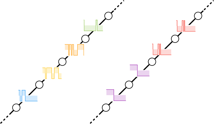
Figure 1: Pictorial representation of the lattice described in Eq. (9), with uncorrelated noise sources (left) and spatially correlated noise (right)

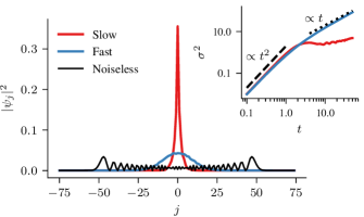
Figure 2: Probability distribution of the walker at $t=50$ for slow ($\gamma=0.01$, red) and fast ($\gamma=1$, blue) noise. The noiseless walker is shown in black for comparison. In the inset, the variance $\sigma^{2}$ as a function of time. The black lines are visual guides for different propagation regimes: ballistic (dashed) and diffusive (dotted). With fast noise we can see a transition from the ballistic to the diffusive propagation, while slow noise causes temporary localization of the walker.

Specifically, in the slow noise regime, also called quasi-static since the percolation rate is very small compared to $J_{0}$, the larger the strength of the noise $\nu$, the more spatially confined the spatial probability distribution is. Localization in quantum walks has been largely addressed in the past years. However those models always considered localization induced by static disorder on the on-site energies of the QW [24, 25, 26, 27] . Model (9) instead shows that localizations can also be due to quasi-static noise on the tunneling energies, thus defying the common concept that only disorder can confine a quantum particle. When the particle localizes, transport through the lattice is suppressed, thus localization is often considered a threat to transfer of an excitation. However, there are situations where localization is deliberately induced in order to keep the walker confined into few sites, thus viewing disorder as a resource more than a threat [37].

In the opposite regime of fast noise, a small strength of the perturbations leads to quasi-unperturbed probability distribution, while larger values make the walker ’classical’, with a Gaussian-shaped distribution, and the system is driven from a ballistic to a diffusive propagation. A qualitatively similar behavior is obtained if the walker is initially prepared in a Gaussian wave packet with a nonzero velocity $p_{0}$ and standard deviation $\Delta$ i.e.,

$$|\psi_{0}\rangle=\sum_{j}\frac{1}{2\pi\Delta^{2}}e^{-\frac{j-N/2}{2\Delta^{2}}}e^{-ip_{0}j}|j\rangle.$$ (10)

This indicates independence of the above results on the initial state of the walker. Moreover, in this case, assuming small strength of the noise, transport through the lattice is possible.

An advantage of the generalized percolation noise model is that it is not specific to the single-particle CTQW. Indeed, it can easily be integrated in a $n$-particle QW model, in order to study the effects of disturbance on the many-body dynamics. For the two-particle case, for instance, the Hamiltonian is:

$$H_{2p}(t)=H_{0}(t)+H_{\text{\tiny int}}$$ (11)

$$H_{0}(t)=\tilde{\mathcal{H}}(t)\otimes\mathbb{I}+\mathbb{I}\otimes\tilde{\mathcal{H}}(t)$$ (12)

where $\tilde{\mathcal{H}}(t)$ is the single particle perturbed Hamiltonian given in Eq. (7) and $H_{\text{\tiny int}}=H_{\text{\tiny int}}(|j-k|)$ is the interaction Hamiltonian, which usually depends on the distance between particles located at sites $j$ and $k$. Different dynamical behaviors arise depending on the statistical nature of the particles, i.e. whether they are bosons or fermions, on their indistinguishability and the noise parameters. Moreover, the initial conditions and the strength of inter-particle interaction are crucial for their time-evolution. Generalized percolation for a two-particle CTQW is analyzed in [38, 39] for on-site and nearest-neighbors interactions. Numerical evidence shows that fast percolation leads to a faster propagation of the initial wave packet of two interacting particles with respect to the noiseless case thus breaking the localization induced by the inter-particle interaction. This means that some components of the wave function gain a larger momentum because of noise and can travel faster across the lattice introducing a new regime that it is not achievable without noise. This behavior is possible only when the particle are initially localized within the range of interaction. In the slow percolation regime localization is induced, with the particles unable to propagate though the lattice.

The model described by Eq.(9) can be further improved by assuming that the tunneling amplitudes can be grouped into spatial domains, with the constraint that all edges within the same domain are synchronized in their fluctuations [40], as depicted in Fig. 1 (right). These spatial regions are called percolation domains. In this case spatial correlations are added to temporal correlations and the autocorrelation function of the noise becomes

$$C(t)\!=\!\begin{cases}e^{-2\gamma t}&\!\!\text{if $j,k$ belong to the same domain}\\ 0&\text{otherwise}\end{cases}.$$ (13)

The spatial domains are created randomly, i.e. if two neighbor edges are correlated with probability $p$, then the probability of creating $M$ domains follows the distribution $P_{M}=\left(\begin{array}[]{cc}N-1\\ M-1\end{array}\right)(1-p)^{M-1}p^{N-M}$. As a consequence, the average length of the domains $\overline{L}=\frac{p^{N}-1}{p-1}$ moves from the case of independent RTN with $\overline{L}=1$, as described in Eq.(9), to the case of uniform noise where all edges percolate synchronously $\overline{L}=N$. The dynamical evolution of the walker is computed as ensemble average not only on the realizations of the noise, but also on the realizations of the randomly generated domains $\rho(t)=\langle U(t)\rho_{0}U^{\dagger}(t)\rangle_{\{J^{\textsc{\tiny T}}_{1}\dots J^{\textsc{\tiny T}}_{M}\}}$.

The dynamics of a Gaussian wavepacket with an initial momentum $p_{0}$ shows that the average velocity of the packet decreases with decreasing average lengths and thus the quantum walker can travel longer across the lattice thanks to spatial correlations. The smaller the value of $\gamma$, the faster this decay is, leading to a full localization in the case $\overline{L}=1$, while the presence of spatial correlations breaks the localization. For bigger values of $\gamma$, on the other side, the effects of large spatial domains is to allow the wavepacket to travel across the graph with an almost unaltered form, i.e. the walker is transfered across the line at fast speed and without losing the information about the initial superposition state. All these results show that spatial correlations can assist the transport of quantum particles over a linear array of nodes.

6 Noisy spatial search by CTQW

In the following, we report recent advancements on the analysis of the robustness of the spatial search algorithm by CTQW [33] against dynamical percolation by RTN. In order to do so, one needs to compare the success probability, i.e., the maximum of Eq. (4) with respect to time, of finding the target in the noiseless and noisy case. The study has focussed on the complete graph and on the star graph, because they both allow for a quadratic speedup of the search in the noiseless case (as seen above), but have very different topological properties. A pictorial representation of the model is shown in Fig. 3. The scaling of the search time with the numbers of nodes $N$ has been studied for various combinations of noise strength $\nu$ and percolation rate $\gamma$.

Let us start with the complete graph. Numerical analysis shows that, depending on the noise regime, different behaviors are found. In particular, for fast noise, the success probability is very close to one even for percolation noise, while slow noise is detrimental for fast search, with a decrease in the success probability. This qualitative result do not depend on $N$, although $p_{w}(t^{\text{\tiny opt}})$ is slightly higher for larger values of $N$. Moreover, the optimal coupling $J=1/N$ remains unaltered regardless of the noise. The role of the noise strength is to reduce the success probability, with full percolation being the worst-case scenario. Interestingly, even if the success probability departs from the optimal one, the algorithm still retains an average speedup over the classical one. Indeed, one can assume that the algorithm can be repeated until the correct result is found, and this happens, on average, after $1/p_{\text{\tiny succ}}$ times, where $p_{\text{\tiny succ}}$ is the success probability. The average running time of the algorithm is still growing as $\mathcal{O}(\sqrt{N})$ even in presence of percolation, as shown in Fig. 4.

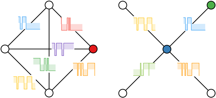
Figure 3: Pictorial representation of the graphs considered for the quantum spatial algorithm: the complete graph (left), where each node is connected to all the others, and the star graph (right), with a central node connected to the remaining ones. In the case of the star graph, we have different results for a central target (blue) or an external target (green), as shown in Fig. 4.

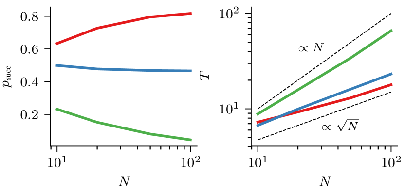
Figure 4: Left: the success probability of the spatial search algorithm as a function of $N$ for slow percolation noise ($\gamma=0.01$, $\nu=1.0$) in the complete graph (red), star graph with central target (blue), star graph with external target node (green). On the right, the scaling of the average running time $T$ with $N$ for the same graphs.

Similar results are obtained in the case of the star graph with the target placed on the central node, but with stronger effects of the noise. Indeed, the optimal coupling is $J=1/N$; the influence of fast noise is almost negligible while slow noise decreases the success probability. The average running time, however, still scales as $\mathcal{O}(\sqrt{N})$, thus the quantum speedup is preserved. This is not the case if the target node is external. The success probability is in general heavily affected by noise, both in the fast and slow percolation regime, as the left panel of Fig. 4 shows. Again, the larger the noise strength, the smaller is the success probability. In this case, the average running time, depending on the strength of the fluctuations, shows a transition from quantum ($\mathcal{O}(\sqrt{N})$) to classical ($\mathcal{O}(N)$) scaling (see Fig. 4, right panel). These results can be interpreted in terms of the connectivity of the two graph topologies: in the complete graph with $N$ nodes there are $N(N-1)/2$ links, while in the star graph there are only $N-1$. While the higher connectivity is not necessary for the noiseless spatial search [47], it allows for greater redundancy in presence of noise. In the limiting case of the star graph with external target node, which is connected to a single edge, noise can completely break the algorithm.

7 Conclusions and perspectives

The concepts of graph and quantum walk are inherently connected, since a CTQW naturally evolves on a graph. In constructing a physical graph, or network, defects and noise may come into play, thus deforming and/or damaging the original structure. The most simple, yet effective, form of perturbation that might affect the topology of a graph is generalized dynamical percolation, where the coupling among the nodes fluctuates in time. A special case of this noise is ordinary dynamical percolation, in which links are created and removed randomly in time. As a matter of fact, generalized percolation modifies the propagation properties of CTQWs on networks, as well as its performance in certain quantum information tasks.

In this perspective article, we have reviewed recent results about the effects of generalized percolation on tasks such as transport on a lattice and spatial search on graphs. The main results is the observation that noise with higher percolation rate leads to faster propagation of the walker. On the other hand, slow percolation favors localization of the particle. This might be a desired behavior in certain situations, but also a drawback in others, such as in the spatial search algorithm.

Links are not the only part of a graph that can be affected by noise. The on-site energies of the nodes may also experience fluctuations, though the corresponding effects are largely unexplored. The presence of diagonal defects has been investigated [41], but a comprehensive study of dynamical noise on the on-site energies is still missing. This is an interesting topic in itself, since it would allow one to understand the role of time-dependent fluctuations compared to static defects, and ultimately shed light on the differences and similarities in the dynamics induced by diagonal and off-diagonal noise. Besides, RTN, i.e. bistable fluctuations, is just one possible model to mimic generalized percolation. Indeed, any stochastic process may be employed to effectively describe noise affecting the coupling constants. Relevant examples are the Gaussian version of a Lorenzian-spectrum noise, i.e. the so-called Ornstein-Uhlenbeck noise, and the class of colored noises, especially the celebrated $1/f$ noise, stemming from a weighted collection of bistable fluctuators.

Generalized percolation is a universal noise model, i.e. it is not specific to a fixed topology, nor to a single-particle CTQW. Any noisy physical system whose evolution can be mapped into a CTQW on a graph [42] may be described using the noise model discussed in this perspective article. Moreover, the same stochastic description may be applied to multi-particle CTQW. Relevant systems where the effects of both time and spatial correlations are worth to investigation are those described Hubbard or Fermi models. In those systems, besides the study of the role of noise in many-body systems, it would be of interest to understand the interplay among particle interaction, statistics and noise in determining the dynamics of the system. As a specific topic of interest, we foresee the possible formation of correlated noisy domains, which would introduce new features in the multi-particle dynamics that are worth exploring.

Another interesting direction for future investigation is the propagation on hypergraphs, i.e. generalization of graphs where hyperlinks connect two or more nodes, instead of just pairs of nodes as in standard graphs. Hypergraphs have been introduced as a more realistic description of real networks and, as such, they call for a careful noise analysis. So far, studies have been focused on the dynamics of discrete-time quantum walks [43] and a question arises on whether CTQW may be defined on hypergraphs, and how generalized percolation affects hyperlinks. Overall, the investigation about the effects of disturbance on the dynamics of a CTQW on hypergraphs is a promising line of research.

As a final remark, we mention that CTQW, which corresponds to a quantum particle moving on a random or noisy graph, may be used as a quantum probe to characterize the graph and its imperfections. In this framework, the added value of using quantum probes to characterize graphs, and the underlying complex quantum systems, is based on the optimisation of the extractable information, as well as the inherently small disturbance introduced into the system itself. In turn, CTQW has been already proved useful to infer the value of the coupling constant of a lattice [44], and of more complex graphs [14].

More generally, being able to characterize properties of networks, including their noise properties, is an essential step in the context of network engineering for quantum information tasks. Indeed, searching for imperfections and defects in a physical network is a crucial step in the implementation and correct functioning of the network itself. In particular, it will be of interest in the near future to investigate how to exploit local quantum measurements on a controllable quantum probe [45] to asses the properties of complex networks instead of resorting to global measurements on the whole graph. Understanding whether CTQW may be used as reliable probes would imply saving resources, such as energy and time, in order to extract precise information about large complex networks.

- [1] \NameY. Aharonov, et al. \REVIEWPhys. Rev. A4819931687.
- [2] \NameE. Farhi and S. Gutmann \REVIEWPhys. Rev. A58 1998915.
- [3] \NameA. M. Childs \REVIEW Phys. Rev. Lett.1022009180501.
- [4] \NameO. Mülken and A. Blumen \REVIEWPhys. Rep. 5022011 37.
- [5] \NameD. Tamascelli, et al. \REVIEWSci. Rep. 62016 26054.
- [6] \NameA. M. Childs, et al.\REVIEWPhys. Rev. A 702004 022314.
- [7] \NameV. Kendon \REVIEWPhil. Trans. R. Soc. A 3642006 3407.
- [8] \NameE. Farhi, et al.\REVIEWTheory Comput. 42008 169.
- [9] \NameJ. K. Gamble et al. \REVIEWPhys. Rev. A 812010 052313.
- [10] \NameS. Cottrell, et al.\REVIEWPhys. Rev. Lett.1122014 030501.
- [11] \NameM. Mohseni, et al. \REVIEWJ. Chem. Phys. 1292008 174106.
- [12] \NameS. Hoyer, et al.\REVIEWNew J. Phys.122010 065041.
- [13] \NameD. Emms et al. \REVIEWPatt. Recogn.422009985.
- [14] \NameL. Seveso, et al.\REVIEW arXiv:1809.092112018.
- [15] \NameH. Schmitz, et al. \REVIEWPhys. Rev. Lett. 1032009 090504.
- [16] \NameR Matjeschk et al. \REVIEWNew J. Phys. 14 2012035012.
- [17] \NameJ. Du et al. \REVIEWPhys. Rev. A672003042316.
- [18] \NameH.B. Perets, et al. \REVIEWPhys. Rev. Lett.1002008170506.
- [19] \NameL. Sansoni, et al. \REVIEWPhys. Rev. Lett.108 2012010502.
- [20] \NameZ.-H. Bian \REVIEWPhys. Rev. A952017052338.
- [21] \NameA. Schreiber, et al. \REVIEWPhys. Rev. Lett.1062011180403.
- [22] \NameA. Romanelli, et al. \REVIEWPhysica A3472005137
- [23] \NameY. Yin, et al.\REVIEWPhys. Rev. A772008022302.
- [24] \NameJ. P. Keating, et al. \REVIEWPhys. Rev. A 762007 012315.
- [25] \NameA. Amir, et al. \REVIEWPhys. Rev. E792009050105R.
- [26] \NameS. R. Jackson, et al. \REVIEWPhys. Rev. A862012022335.
- [27] \NameA. Croy, et al. \REVIEWEur. Phys. J. B822011107.
- [28] \NameS. D. Druger et al. \REVIEW J. Chem. Phys.7919833133.
- [29] \NameT. G. Wong, et al. \REVIEWQuantum Inf. Process.1520164029.
- [30] \NameF. A. Cuevas, et al. \REVIEWAnn. Phys.32620112834.
- [31] \NameN. Konno \REVIEWPhys. Rev. E722005026113.
- [32] \NameE. Farhi, et al. \REVIEWPhys. Rev. A571998 2403.
- [33] \NameM. Cattaneo, et al. \REVIEWPhys. Rev. A982018052347.
- [34] \NameZ. Darázs, et al. \REVIEWJ. Phys. A462013375305.
- [35] \NameE. Piccinini, et al. \REVIEWComp. Phys. Comm.2152017235.
- [36] \NameC. Benedetti, et al. \REVIEWPhys. Rev. A932016042313.
- [37] \NameL. Sapienza, et al. \REVIEWScience32720101352.
- [38] \NameI. Siloi, et al. \REVIEWPhys. Rev. A952017022106.
- [39] \NameI. Siloi et al. \REVIEWJ. Phys.: Conf. Ser.9062017012017.
- [40] \NameM. A. C. Rossi, et al. \REVIEWPhys. Rev. A.962017040301.
- [41] \NameJ. A. Izaac, et al. \REVIEWPhys. Rev. A882013042334
- [42] \NameA. Hines,et al. \REVIEWPhys. Rev. A752007062321.
- [43] \NameY. Liu, et al. \REVIEWSci. Rep820189548.
- [44] \NameD. Tamascelli, et al. \REVIEWPhys. Rev. A942016042129.
- [45] \NameJ. Nokkala, et al. \REVIEWSci. Rep. 8201813010.
- [46] \NameM. A. C. Rossi, et al. \REVIEWarXiv:1811.047802018.
- [47] \NameD. A. Meyer et al. \REVIEWPhys. Rev. Lett.1142015110503