SOC program for dust continuum radiative transfer

Abstract

Context. Thermal dust emission carries information on physical conditions and dust properties in many astronomical sources. Because observations represent a sum of emission along the line of sight, their interpretation often requires radiative transfer modelling.

Aims. We describe a new radiative transfer program SOC for computations of dust emission and examine its performance in simulations of interstellar clouds with external and internal heating.

Methods. SOC implements the Monte Carlo radiative transfer method as a parallel program for shared memory computers. It can be used to study dust extinction, scattering, and emission. We tested SOC with realistic cloud models and examined the convergence and noise of the dust temperature estimates and of the resulting surface brightness maps.

Results. SOC has been demonstrated to produces accurate estimates for dust scattering and for thermal dust emission. It performs well with both with CPUs and with GPUs, the latter providing up to an order of magnitude speed-up. In the test cases, ALI improved the convergence rates but also was sensitive to Monte Carlo noise. Run-time refinement of the hierarchical-grid models did not help in reducing the run times required for a given accuracy of solution. The use of a reference field, without ALI, works more robustly. It also allows the run time to be optimised if the number of photon packages is increased only as the iterations progress.

Conclusions. The use of GPUs in radiative transfer computations should be investigated further.

1 Introduction

Most knowledge of astronomical sources is based on radiation that is produced and processed by inhomogeneous objects viewed from a single viewpoint. This also applies to interstellar medium, the line emission from gas and the continuum emission from interstellar dust. Radiative transfer (RT) defines the relationships between the physical conditions in a radiation source and the observable radiation. Thus, RT modelling is needed to determine the source properties or, more generally, the range of properties consistent with observations.

Many RT programs exists for the modelling of dust continuum data (e.g. Bianchi et al. 1996; Dullemond & Turolla 2000; Gordon et al. 2001; Bjorkman & Wood 2001; Juvela & Padoan 2003; Steinacker et al. 2003; Wolf 2003; Harries et al. 2004; Ercolano et al. 2005; Juvela 2005; Pinte et al. 2006; Jonsson 2006; Chakrabarti & Whitney 2009; Robitaille 2011; Lunttila & Juvela 2012; Natale et al. 2014; Baes & Camps 2015) and benchmarking projects have quantified the consistency between the different methods and implementations (Ivezic et al. 1997; Pascucci et al. 2004; Gordon et al. 2017). Part of these codes can also be used in studies of polarised scattered or emitted radiation (Whitney et al. 2003; Pelkonen et al. 2007; Bethell et al. 2007; Reissl et al. 2016; Peest et al. 2017).

RT is computationally demanding because each source location is in principle coupled with all the other positions (Steinacker et al. 2013), the coupling changing with wavelength. Emission calculations may need iterations where temperature estimates and estimates of the radiation field are updated alternatingly. Most codes for dust emission and scattering modelling are based on the Monte Carlo method, the simulation of large numbers of photon packages that represent the actual radiation field. In “immediate re-emission” codes (Bjorkman & Wood 2001), every interaction with the medium leads to a re-evaluation of the dust emission from the corresponding model cell. In other Monte Carlo codes the information about the absorbed energy is stored during the simulation step, after which the temperatures of all cells are updated. Models with high dust temperatures and high optical depths may require a significant number of iterations.

In the case of large 3D models, the run times become long and some parallelisation of the computations may be necessary (Robitaille 2011; Verstocken et al. 2017). The Monte Carlo method allows straightforward parallelisation of the radiation field simulations, at the level of individual photon packages or between frequencies (if the basic simulation scheme this allows) or even based on the decomposition of the computational domain (Harries 2015). However, naive parallelisation – where each computing unit performs independent simulations with different random numbers – may also be the most efficient.

The parallelisation between nodes is typically handled with Message Passing Interface (MPI) and within a node (on a single shared-memory computer), for example, with OpenMP, lower level threads, or other language-specific (or vendor-specific) tools. Further speed-up could be obtained with graphics processing units (GPUs) that theoretically are capable of more floating point operations per second than even high-end CPUs. The use of GPUs has been hindered by the more complex programming model and the limited device memory. However, the massive parallelism provided by GPUs is well suited for radiative transfer calculations and some applications to astronomical radiative transfer already exist (Heymann & Siebenmorgen 2012; Malik et al. 2017). These use the CUDA parallel programming platform, which is proprietary to NVIDIA and cannot be used with GPUs of other manufacturers. Furthermore, CUDA programs are written explicitly for GPUs and cannot be run on CPUs. GPU programming is becoming more approachable as directive-based programming models are becoming available. The support for GPUs (and “accelerators” such as Intel Xeon Phi, AMD Radeon Instinct, etc.) is maturing in OpenMP. This enables heterogeneous computing, the same program running on both GPUs and CPUs. However, in this paper we describe the continuum radiative transfer program SOC that is written using OpenCL libraries. OpenCL is an open standard for heterogeneous computing. Thus, SOC can in principle be run unaltered on CPUs, GPUs, and even other accelerators. OpenCL is supported by many vendors and, furthermore, has fully open source implementations, making it more future-proof against the current rapid changes and evolution of the GPU computing frameworks.

SOC has been compared to other continuum radiative transfer programs in Gordon et al. (2017). In this paper we describe in more detail some of the implementation details and examine the efficiency of SOC and some of the implemented methods in the modelling of dust emission from interstellar clouds clouds. In a future paper, SOC will be used to produce synthetic surface brightness maps for a series of MHD model clouds and, based on these, to construct synthetic source catalogues with the pipeline used for the original Planck Galactic Cold Cores Catalogue (PGCC) (Planck Collaboration et al. 2016). One of these MHD models is already used in the tests in the present paper.

The contents of the paper are the following. In Sect. 2 we discuss the implementation of the SOC programme. In the results section Sect. 3, we describe tests on the SOC performance. These include in particular problems that require iterations to reach final dust temperature estimates (Sect. 3.3-3.4). The findings are discussed in Sect. 4 and the final conclusions are listed in Sect. 5. In Appendix A we discuss further the calculation of emission from stochastically heated grains.

2 Methods

In this section, we present some details of the SOC implementation and the model clouds used in the subsequent tests.

2.1 SOC radiative transfer program

SOC is a Monte Carlo radiative transfer program for the calculation of dust emission and scattering. It has been used in some publications (Gordon et al. 2017; Juvela et al. 2018b, a) but we describe here in more detail some of the implementation details.

2.1.1 Basic program

SOC uses OpenCL libraries, enabling the program to be run on both CPUs and GPUs. This has affected some of the design decisions. The program is run on a $host$, which calls specific routines, called kernels, that are executed on a $device$. The host is the normal computer (CPU) while the device can be a CPU (using the same resources as the host), a GPU, or other accelerator. Thus, the memory available on the device may be more limited than usual. SOC has separate kernels to carry out the simulation of photon packages at a single frequency, to solve the dust temperatures based on the computed absorbed energy (non-stochastically heated grains only), and, based on that solution, to produce surface brightness maps at given frequencies.

In Gordon et al. (2017) we used an earlier version that employed modified Cartesian grids. Current SOC uses cloud models defined on hierarchical grids. The root grid is a regular Cartesian grid with cubic cells. Refinement is based on octrees where each cell can be recursively divided into eight sub-cells of equal size. In the following we refer to such a set of eight cells as octet and the number of hierarchy levels as $n_{\rm L}$. The root grid is the level $L=1$ and a grid consisting only of the root grid has $n_{\rm L}$=1. The cells of the model cloud form a vector that starts with the cells of the root grid, followed by all cells of the first hierarchy level, an so forth. The links from parent cells to the first cell in the sub-octet are stored in the same structure, encoding the index of the first child cell as a negative value in place of the density value in the parent cell. Because each octet is stored as consecutive elements of the density vector, smaller auxiliary arrays are sufficient to store the reverse links from the first cell of an octet to its parent cell. Neighbouring cells could be located faster by using explicit neighbour lists (Saftly et al. 2013). However, to reduce memory requirements, an important consideration especially on GPUs, we are currently not using that technique. Therefore, each time a photon package is moved to a new cell, a partial traversal of the hierarchy is required, up to a common parent cell and then down to the new leaf node that corresponds to the next cell along the path of the photon package.

The SOC program is based on the usual Monte Carlo simulation where the radiation field is simulated using a pre-determined number of photon packages, each standing for a large number of real photons. SOC concentrates on the radiative transfer problem and does not have built-in descriptions of specific dust models, radiation sources, or cloud models (density distributions). These inputs are read from files that are specified in the SOC initialisation file. They include the cloud hierarchy with the density values, the dust cross sections for absorption and scattering, and scattering functions tabulated as functions of frequency and scattering angle.

The simulation is done using a fixed frequency grid. Therefore, at each step of the calculations, the kernel only needs data related to a single frequency. These include the densities and, for the current frequency, the optical depth and a counter for the number of absorbed photons. The density vector (one floating point number per cell) includes basic information about the grid geometry. The information about parent cells is less than one eight of this (link for first cell of each octet, excluding the root level). The host sets up the data for the current frequency and these are transferred to the device. After the kernel has completed the simulation of the radiation field, the information of the number of absorptions in each cell can be returned to the host. The host loops over simulated frequencies, calls the kernel to do the simulations, and gathers information of absorption events.

For stochastically heated grains, the information about absorbed energy is converted to dust emission using an external programs such as DustEM (Compiègne et al. 2011) or the program we used in Lunttila & Juvela (2012) and in Camps et al. (2015). On the host side this requires the storage of large arrays that, for modern computers, would not set serious limits to the size of the computed models. However, in SOC these are stored as memory-mapped files. Memory-mapped files reside on disk but can be used in the program transparently as normal arrays. The operating system is responsible for reading and writing the data, as needed, without the data ever being in the main memory all at the same time. Thus the main limitation remains the device memory and the amount of data per a single frequency.

If grains are assumed to be in an equilibrium with the radiation field, the emission is calculated by SOC itself, again using a separate kernel. The integral of the absorbed energy over frequency can be gathered directly during the simulations, without the need for large multi-frequency arrays. The absorption information remains on the device, and only the computed dust emission is returned to the host. As the final step, the host calls a mapping kernel to make surface brightness maps for the desired frequencies and directions.

SOC can also produce images of scattered light. However, these are usually made with separate runs that employ methods such as forced first scattering, peel-off, and potentially additional weighting schemes (Juvela 2005; Baes et al. 2016). Apart from the use of different spatial discretisation, SOC results for scattering problems have already been discussed in Gordon et al. (2017). We concentrate in this paper on the dust emission and especially the methods described in the next section.

2.1.2 Additional methods

SOC implements some features beyond the basic Monte Carlo Scheme. These include forced first scattering and accelerated lambda iterations (ALI). ALI (also called accelerated Monte Carlo or AMC) is computed using a diagonal operator that solves explicitly for the cycle of photons that are absorbed within the emitting cell (see Juvela 2005). The use of ALI incurs an additional cost of storing on the device one additional floating point number per cell, which is needed to keep track of the photon escape probabilities for each cell. SOC includes optional weighting for the scattering direction (Juvela 2005) and the step length between scattering events. The latter is similar in nature to the method described in (Baes et al. 2016) but, to avoid explicit integration to the model boundary, the probability distribution of the simulated free path is based on the sum of two exponential functions of optical depth, with user-selected parameters. The weighting is applied only on the first step of each photon package.

SOC can use a reference field to reduce the noise, especially in calculations that involve several iterations (Bernes 1979; Juvela 2005). In this method, each simulation step only estimates a correction to the average radiation field determined by the previous iterations. This requires that the absorptions caused by the reference field are also stored, adding storage requirements by one number per each cell and frequency. For grains at an equilibrium temperature, this reduces to a single number per cell (the total absorbed energy). In an ideal case, the overall noise would then decrease as $n_{\rm I}$^-1/2, as the function of the number of iterations – assuming that the number of photon packages per iteration, $n_{\rm P}$, is constant. However, because also the temperatures change during the iterations, the noise is likely to decrease more slowly, especially during the first iterations.

Iterations are needed if the model includes high optical depths and dust is heated to such high temperatures that its emission no longer freely escapes the model volume. In the context of interstellar clouds, this means dust near embedded radiation sources, possibly in a very small fraction of the whole model volume. In these cases, the reference field can be used for further optimisation. After the first iteration, the reference field already contains the information of all constant sources, such as the embedded point sources or the background radiation, and they can be omitted from the subsequent iterations. Furthermore, it is possible to divide the cells to two categories. Passive cells are those whose emission (resulting from their temperature change during the iterations) is too low to affect the temperature of other cells. Active cells are correspondingly those whose temperature does change with iterations, affecting the temperature of other cells. Once the former are included in the reference field (if their emission indeed is significant at all), on subsequent iterations only emission from the active cells needs to be simulated. In SOC, the host can examine the changes of emission between iterations and can thus omit the creation of photon packages for cells for which the emission has not changed. However, in practice the same is accomplished by weighted sampling where the number of photon packages emitted from each cell is determined by the cell luminosity.

Finally, SOC has the option to change the spatial resolution also during iterations. One could start with a low-resolution model, doing fast iterations, and only later refine to the final resolution needed. This could result in savings in the run times, depending on the optical depths and the intensity of the dust re-emission. On the other hand, a lower spatial resolution means optical depths for individual cells, which tends to slow the convergence of temperature values down, especially when ALI is not used. The run-time refinement is briefly tested in Sect. 3.4

The present SOC does not carry out the radiative transfer simulation with polarised radiation but can nevertheless be used to calculate synthetic maps of polarised dust emission. SOC can determine for each cell the intensity and the anisotropy of the radiation field. Other scripts are used to calculate the resulting polarisation reduction factors, for example, according to the radiative torques theory, thus also including the information about the magnetic field orientation. The procedure is essentially identical to the computations presented in Pelkonen et al. (2009). The information of the polarisation reduction and of the magnetic field geometry are read into SOC, which then produces synthetic maps of the Stokes parameters. The calculations ignore the effects on the total intensity that result from the cross sections being dependent on the angle between the magnetic field and the direction of the radiation propagation. This is usually not a severe approximation (especially when compared to the many other sources of uncertainty). However, based on SOC, another program is now in preparation where all calculations are done using the full Stokes vectors, taking into account the degree to which the grains are in each cell aligned with the magnetic field (Pelkonen 2018 in preparation).

2.2 Test model clouds

The first tests were performed with spherically symmetric density distributions that were sampled onto hierarchical grids (see Sect. 3.1).

Most tests employed a snapshots from the MHD simulations described in Padoan et al. (2016b), which has already been used for synthetic line observations of molecular clouds (Padoan et al. 2016a) and for studies of the star-formation rate (Padoan et al. 2017). These simulations of supernova-driven turbulence were run with the Ramses code (Teyssier 2002), using a 250 pc box with periodic boundary conditions. The runs started with zero velocity, a uniform density $n{\rm(H)}$=5 cm^-3, and a uniform magnetic field of 4.6 $\mu$G. The self-gravity was turned on after 45 Myr and the simulations were then run for another 11 Myr. In the hierarchical grid, the largest cell size is 0.25 pc but in high-density regions the grid is refined down to $7.6\times 10^{-3}$ pc. In this paper, we use a (10 pc)³ sub-volume selected from the full (250 pc)³ model cloud. Table 1 lists the number of cells on each level of this (10 pc)³ model with maximum refinement $n_{\rm L}$=7. The largest number of cells is found on the level $n_{\rm L}$=4. Figure 1 shows examples of surface brightness maps computed for models with $n_{\rm L}$=1-4.

The radiative transfer problem is solved with SOC, assuming an external radiation field according to Mathis et al. (1983) (solar neighbourhood values) and dust properties given by Compiègne et al. (2011). We use a fixed frequency grid that has 52 frequencies that are placed logarithmically between 10¹¹ Hz and $3\times 10^{15}$ Hz (between 0.1 $\mu$m and 3000 $\mu$m). Tests are are made assuming that the grains remain in temperature equilibrium with the radiation field.

Even with external illumination only, the radiation field intensity does not have significant large-scale gradients in the MHD cloud models. This is caused by the inhomogeneity of the models which leads to a relatively uniform intensity in the low-density medium. Strong temperature variations are seen but mainly at smaller scales, in connection with individual high-column-density structures. Apart from the background radiation, the other potential radiation sources are internal sources (modelled as a blackbody point sources) and the re-emission from the heated dust itself.

Table 1: Number of cells on each hierarchy level of the (10 pc)³ model clouds with $n_{\rm L}$=7.

Hierarchy level $L$	Number of cells
1	8000
2	49176
3	185232
4	365184
5	295824
6	178280
7	83632

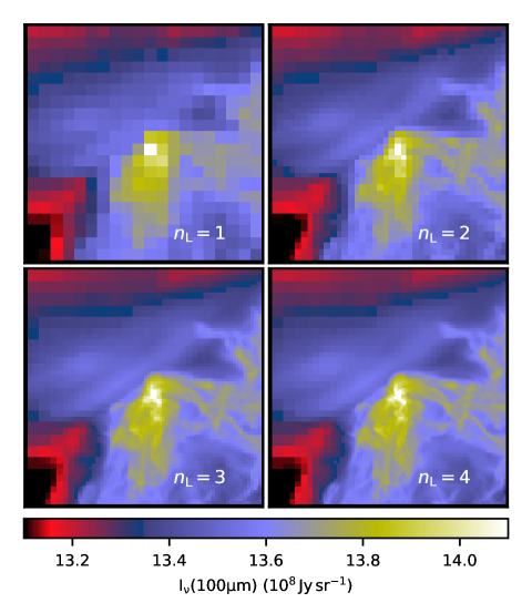
Figure 1: Examples of 100 $\mu$m surface brightness maps computed for 3D model clouds with a maximum refinement to $n_{\rm L}$=1-4 hierarchy levels. In calculations involving internal heating (as in these examples), point source is placed in an empty root grid cell at the centre of the model volume.

3 Results

To examine the performance of SOC in simulations of external and internal radiation sources and of dust emission, we start with tests with simple spherically symmetric model clouds (Sect. 3.1). In Sect. 3.2, we continue with more realistic models based on a MHD simulation. Finally, the more demanding iterative computations with internally heated and optically thick clouds is discussed in Sect. 3.3.

To make the results more concrete, we quote timings for a laptop that has a six-core CPU and a dedicated GPU. The performance is measured in terms of the wall-clock time, the actual time that has elapsed, for example, between the start and the finish of a run.

3.1 Tests with spherical model clouds

First tests were conducted with small, spherically symmetric models resampled onto a hierarchical grid. The root grid is 17³ cells and is refined to $n_{\rm L}$=2-5 levels with some 5000 cells per level. Thus about one eight of the cells is refined and the total number of cells is only $\sim$10000 - 20000, depending on $n_{\rm L}$. A 10000 K blackbody point source with a luminosity of $L=1\,L_{\sun}$ is located at the centre, in a root grid cell with zero density. Otherwise the density profile is gaussian with a density contrast $\sim$200 between the centre and the edges. The maximum column density is $N({\rm H_{2}})\sim 1.3\times 10^{23}$ cm^-2, slightly depending on the discretisation used. We characterise the noise of the calculations by using the random mean squared (rms) noise of the resulting 100 $\mu$m maps.

Figure 2 shows how the results change as a function of the number of simulated photons packages and the model refinement. The results show the expected $N^{-0.5}$ dependence of the noise on the number of photon packages, irrespective of the depth or the grid hierarchy. This applies to the simulations of the point source, the diffuse background, and the emission from the medium itself. Each map has a pixel size that corresponds to the smallest cell size of that particular model. With larger $L$, the maps become more over-sampled (especially towards the map edges), which has some effect on the computed rms values. The actual noise per 3D cell measured by the dust temperature is in refined regions proportional to $2^{L}$ because the number of photon packages hitting a cell decreases by a factor of 4 for each additional level of the grid hierarchy.

Figure 2b compares results to the map obtained with the highest refinement and the highest number of photon packages. The differences are completely dominated by the difference in discretisation. The dependence on the number of photon packages is visible only when comparing runs with the same gridding.

The last column in Fig. 2 shows the wall-clock run times, including initialisations and the writing of the surface brightness maps for all frequencies. The map size in pixels depends on the discretisation but the effects for the overall run times are not significant. On the test computer, the speed-up provided by the GPU varies from $\sim 50$% (for small number of packages, when the initialisation overheads are significant) close to a factor of ten. The behaviour is qualitatively similar for lower column density models where there are fewer multiple scatterings and the cost associated to the creation of photon package is larger relative to the tracking of the photon paths. The speed-up of GPU relative to CPU increases with the number of photon packages, except for the point source simulations. Possible reasons for this are discussed in Sect. 4.2.

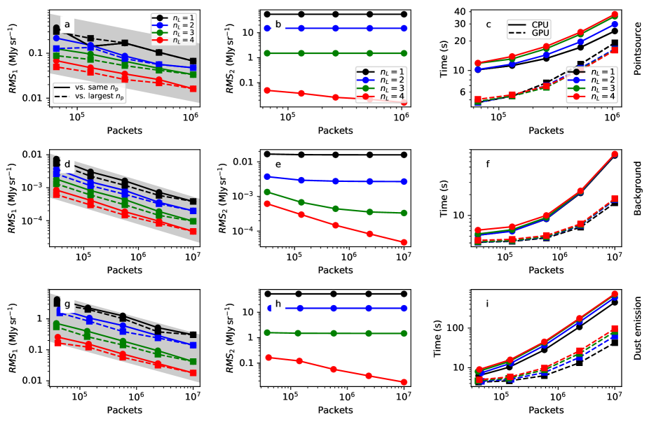
Figure 2: Noise and run times as a function of the number of photon packages for a small spherically symmetric test model. Results are shown for simulations of a point source (frames a-c), a diffuse background (frames d-f), and the dust emission from the model volume (frames g-i). The first column shows the rms noise of the 100 $\mu$m map as the difference of two identical runs (solid lines) and from the comparison to a run with the same volume discretisation (same $n_{\rm L}$) but the highest number of photon packages (dashed lines). Shading is used to indicate the expected $n_{\rm P}$^-1/2 convergence as a function of the number of photon packages. The second column shows the rms difference to a corresponding run with the highest number of photon packages $and$ the finest spatial discretisation ($n_{\rm L}$=5). The wall-clock run times for CPU (solid lines) and GPU (dashed lines) computations are shown in the last column. In each frame, the colours correspond to different values of $n_{\rm L}$, as indicated in frame c.

3.2 Tests with 3D model clouds

The next tests involve a 3D model based on MHD simulations (see Sect. 2.2). We analyse maps that are computed towards the three cardinal directions. The map pixel size corresponds to the smallest model cells. The 10 pc$\times$10 pc projected area is thus covered by maps with 1310$\times$1310 pixels. The average column density is $N({\rm H}_{2})\sim 2.4\times 10^{21}$ cm^-2 ($A_{\rm V}=2.3$ mag) and the maximum column density ranges from $1.78\times 10^{23}$ cm^-2 ($A_{\rm V}=172$ mag) to $2.46\times 10^{23}$ cm^-2 ($A_{\rm V}=238$ mag), depending on the view direction. The values of visual extinction $A_{\rm V}$ given in parentheses correspond to the dust model used in the simulations.

The model volume is centred on a site that will give birth to a high-mass star. However, in these tests we run the models either without internal heating or using a radiation source that is located in the star-forming core but has an ad hoc luminosity that is made so high that the dust temperatures converge only after several iterations.

We start by checking how the noise behaves as a function of the number of photon packages or the run time. Compared to Sect. 3.1, the grid is now fixed but the model size is closer to that of potential real applications. Figure 3 shows the results for a single iteration. The noise decreases mostly approximately according to the $n_{\rm P}^{-1/2}$ relation. In the case of a point source, the convergence is slightly faster because with lower package numbers some cells at the model boundaries may not be hit at all. These cells get assigned an ad hoc constant temperature and, in spite of their low number, have an impact on overall noise values.

Plots contain two relations for dust re-emission. In the default method, the same number of photon packages is sent per each cell (with random locations and directions within each cell). For uniform sampling, SOC also requires the number of photon packages (per frequency) to be a multiple of the number of cells. Therefore, results for runs with smaller number of requested photon packages end up at the same location in the plot with actual number of photons packages just above $n_{\rm P}\sim 10^{6}$. The other relations (open symbols) correspond to simulations where the number of emitted photon packages is weighted according to the emission. These runs include, as constant contributions, the heating from previous simulations of the external radiation field and the point source. Hot dust (temperature above 100 K) is found only near the central source. The convergence is slower than $n_{\rm P}^{-1/2}$ because, in the case of emission weighting, the maximum number of photon packages sent from any single cell was limited to 10000 with a user-defined parameter. Such a cap may be sometimes necessary to ensure proper sampling also for the emission from cooler dust, which could be important locally in regions far from the hottest dust. On the other hand, an increase in $n_{\rm P}$ will not improve the accuracy with which one simulates the emission from cells that have already reached the cap value.

Apart from constant overheads at small photon numbers, the run times are generally directly proportional to $n_{\rm P}$. The speed-up provided by the GPU is $\sim$4 in the pointsource and background radiation simulations and slightly higher for the standard dust re-emission calculation. The situation is very different when emission weighting is used. Compared to the unweighted case, the run times are shorter on CPU while on GPU they are longer. This is discussed further in Sect. 4.2.

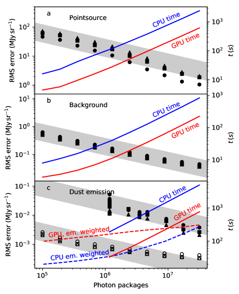
Figure 3: Test with high-resolution model in the case of only a point source (frame a) or only background radiation (frame b), or including both as constant radiation field components to examine the noise in the simulation of dust re-emission. The rms errors as a function of the number of photon packages are shown with black symbols. The circles, squares, and triangles correspond to maps calculated toward three orthogonal directions. The shading shows the expected $N^{-1/2}$ convergence. The lines and right hand y-axis indicate the run times for CPU (blue) and GPU (red). In frame c, open symbols and dashed lines correspond to an alternative run with emission weighting.

Without photon splitting or similar techniques, each additional level of the hierarchy should decrease the probability of photon hits by a factor of four. Thus, the noise should increase proportionally to $2^{L}$, where $L$ is the grid level (larger $L$ standing for smaller cells). Figure 4 shows the actual rms error of dust temperatures as a function of the hierarchy level. The $2^{L}$-dependence holds for the background radiation. In the pointsources simulation, the noise is constant or even decreases at the highest levels because those cells are on average closer to the source. For the simulated dust re-emission, the noise values are lower but increase rapidly on the highest refinement levels. This is partly an artefact of the model setup where the cells on low grid levels are heated mainly by sources other than the dust re-emission and therefore in this test have a low noise. The emission-weighting leads to lower noise values that also are more uniform between cells of different size.

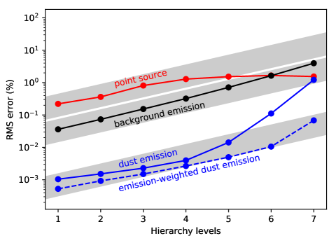
Figure 4: Error of the computed dust temperatures as a function of the grid hierarchy in a model with $n_{\rm L}$=7. From top to bottom, the curves correspond to simulations of a point source (red curve), heating by background radiation (black curve), and simulations of dust emission when the contribution of the previous radiation sources is kept constant (blue curves). The solid and dashed lines correspond to the default and the emission-weighted simulations, respectively. The shaded regions are used to illustrate the expected $2^{\rm level}$ dependence of the noise. All calculations were done with $1.8\times 10^{7}$ photon packages per frequency.

Run times should be proportional to the number of cells (assuming that the sampling of the radiation field is kept uniform) but, in our case, deeper grid hierarchies are associated with some overhead in the tracking of the photon packages. Figure 5 shows the run times as a function of the number of cells in models that are refined down to $n_{\rm L}$=1-7. The number of photon packages is kept at $1.8\times 10^{7}$ so that plot shows only the effect of discretisation. In the plot, the run times increase slower than the number of cells because cells at higher hierarchy levels are hit by progressively fewer photon packages. To ensure a certain SNR level even for the refined regions, the number of photon packages should be proportional to $2^{n_{\rm L}}$ (Fig. 4). An increase in the overhead is visible for deeper hierarchies with $n_{\rm L}$=5-7 although the run times are still almost proportional to the number of cells. As indicated by Table 1, even though the tracing of the photon paths through cells at high refinement levels were significantly slower, the effect on the total run times is limited because of the small fractional number of those cells. Some GPU runs appear to deviate from the general trends. Emission-weighted simulations of dust re-emission slow down for deeper hierarchies (see Fig. 3 and discussion above) and for $n_{\rm L}$=5-7 are similar to the CPU run times. Furthermore, point source simulations suffer from coarse discretisation ($n_{\rm L}$$<$=4), possibly because of the locking overheads for global (multiple threads doing frequent updates to the same cells close to the point source).

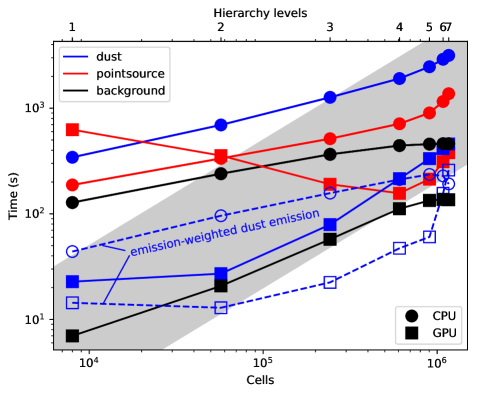
Figure 5: Dependence of run times on the maximum refinement. The colours correspond to simulations of the radiation from a point source (red), external background (black), and dust re-emission (blue). For dust emission, the dashed lines and open symbols correspond to a run using emission weighting. The CPU run times are plotted with circles and the GPU run times with squares. The shading indicates the trend for run times proportional to the number of cells.

3.3 Iterative solution of dust temperature

Above we were only concerned with the simulations of the radiation field. For optically thick models and especially in the case of internal radiation sources, the question of the convergence of the temperature values becomes equally important. Calculations could be sped up by reducing the number of iterations required for a converged solution or by reducing the time per iteration.

We first examine the performance of the ALI method as a function of the model discretisation. We are using ALI with a diagonal operator that only separates the absorption-emission cycles within individual cells. The effects should depend on the discretisation. Higher spatial resolution means that the optical depth of individual cells is smaller and thus we can expect less benefit from the use of ALI.

We use the same density field as in Sect. 3.2 and a single internal radiation source. The original model described a (10 pc)³ volume where the effects of an even very luminous source would remain local. Therefore, in this test the linear size of the cloud was decreased by a factor of 20, the densities were increased by a factor of 100, and the luminosity of the radiation source set so that the temperature of the closest cells is hundreds of degrees. These ensure that dust re-emission is important over a larger volume and that the dust temperatures converge only after many iterations. The setup is only used to test the radiative transfer methods and is not supposed to be a physically accurate description of a star-forming core.

Figure 6 shows the convergence of temperature values for the $n_{\rm L}$=4 model for runs with $n_{\rm P}$$\sim 18\times 10^{6}$. The convergence is measured based on the average dust temperatures on only the highest level of refinement (thus cells close to the point source), comparing these to a non-ALI run with the same $n_{\rm P}$  and 40 iterations. Based on the rate of convergence in Fig. 6, the error of that reference should be two orders of magnitude smaller than on the final iterations shown in the figure.

The average temperature is initially increasing by $\sim$10 K per iteration. After 20 iterations, this rate has decreased by a factor of one hundred. ALI leads to a faster convergence and the rate of convergence is about the same for all cells, irrespective of their location with respect to the point source. In run times, the overhead of ALI is some 5%, which is more than compensated by the faster convergence. The rms errors are similar with and without ALI.

Figure 6 shows further how, depending on the requirements on accuracy (bias and random errors), the run times could be significantly shortened simply by reducing the number of photon packages. The rms errors are naturally higher but this does not affect the initial rate of convergence measured using $|\langle\Delta T\rangle|$. However, with low photon numbers, the convergence stops earlier and also the bias of the final temperature estimates is larger. When $n_{\rm P}$  is reduced by a factor of 64, the final bias is $\Delta\langle T\rangle\sim$1 K. The bias is even more significant in the resulting surface brightness maps, analogous to the way LOS temperature variation bias observational dust temperature estimates (Shetty et al. 2009; Juvela & Ysard 2012). Figure 6.

In Fig. 6b the convergence of the ALI runs saturates at a level $|\langle\Delta T\rangle|\sim 0.1$ K. Qualitatively this could be expected based on the above results with lower photon number. However, we measure convergence with respect to a reference solution that is calculated with 40 iterations but without ALI. Like the low-photon-number runs, the reference solution will have a systematic error that is larger than suggested by the extrapolation of the initial linear trend in Fig. 6b. The fact that the $|\langle\Delta T\rangle|$ curve of the ALI run flattens relative to that reference solution suggests that ALI may be more sensitive to Monte Carlo noise.

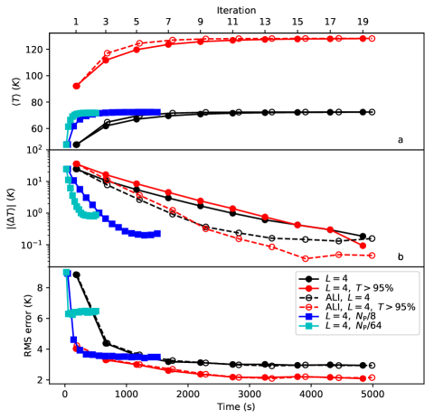
Figure 6: Convergence of dust temperature values as a function of iterations and the run time on CPU. Temperatures are from the cells on the finest level of refinement of a model with $n_{\rm L}$=4. Frame a shows the average temperature for basic runs (solid lines) and for ALI runs (dashed lines and open symbols). Black line is the average for all cells on the level $L$=4 and the red curve is for 5% of the cells with the highest temperatures. The blue and cyan curves correspond to the average of all $L=$4 cells in runs with reduced number of photon packages $n_{\rm P}$. Frame b shows the errors relative to a run with 40 iterations and without ALI. Frame c shows the rms errors for $L=4$ cells calculated as the standard deviation between two independent runs.

The emission maps and error maps for the final iteration of Fig. 6 are shown in Appendix B.

3.4 Faster iterative solutions

When the convergence of temperature values requires many iterations, the calculations can be sped up in at least three ways. These include the use of sub-iterations, the use of a reference field, and run-time model refinement.

The idea behind sub-iterations is that temperature updates are sometimes restricted to an “active” subset of cells whose temperatures and temperature changes are most relevant for the final solution. This results in savings in the simulation step, because emission is re-simulated only from a fraction of all cells, and in the temperature updates, which are similarly restricted to a subset of cells. Some overhead is caused by the necessity to use a reference field to store the contribution of other cells to the total radiation field. We do not test this method here because emission weighting provides similar savings in the simulation step. Because our tests do not include stochastically heated grains, the contribution of temperature updates to the total run times is at the level of only one per cent. For stochastically heated dust, the run times could be dominated by the calculation of the temperature distributions (see Appendix A) and a simpler version of sub-iterations can be implemented simply by skipping the temperature updates for weakly-emitting cells.

The use of a reference field enables speed-up because, for a given final noise level of the solution, the number of photon packages per iteration can be lower. In the case of a hierarchical grid, the most refined regions tend to have both the highest noise and the slowest convergence. Therefore, some care must be taken to ensure that the solution has truly converged in those regions.

Figure 7 shows results for the $n_{\rm L}$=4 model when using a reference field. This can be compared to the previous plots of the rms noise in Fig. 4 and the convergence in Fig. 6. The setup is identical (including background and a point source and constant radiation sources) but the number of photon packages per iteration has been decreased by a factor of 16. Examples of the corresponding surface brightness maps can be found in Appendix B.

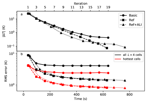
Figure 7: Results for $n_{\rm L}$=4 model when using a reference field. All statistics refer to the average dust temperature of the cells on the highest $L$=4 level of the grid hierarchy. Frame a shows the temperature error relative to the solution obtained with the same setup after 20 iterations. Frame b shows the rms temperature difference between two independent runs, the red curves showing these separately for 5% of the cells with the highest temperatures. Circles stand for the basic calculations (no ALI and no reference field), squares to a reference field runs, and triangles to the combination of the reference field and ALI techniques. Values are plotted against the run time and the upper x-axis shows the corresponding number of iterations in the basic run.

The run times are significantly shorter than in Fig. 6 but only by a factor of $\sim 6$ rather than the factor of 16 between the number of photon packages. This is caused by the non-linearity seen in Fig. 2i, the lower efficiency of simulations with low photon numbers that should disappear for sufficiently large photon numbers. The convergence rate in Fig. 7b should depend only on the use of ALI. ALI results in smaller $\Delta T$ errors but the difference is smaller than in Fig. 6b, probably because the larger noise on the first iteration decreases the efficiency of ALI corrections. The effect of a reference field is seen in Fig. 7b where it decreases that final rms error by a factor of $\sim 3$. The combination of ALI and a reference field increases the run times per iteration by close to 30% while the reference field alone is not associated with any overheads.

3.5 Run-time grid refinement

Before discussing tests with run-time model refinement, Fig. 8 shows for how dust temperature errors depend on the number iterations and the number of hierarchy levels ($n_{\rm L}$). Neither ALI not a reference field is being used and the discretisation is constant throughout the calculations that each correspond to one row in the plot. The plot only measures the errors related to the convergence of temperature values. The errors are calculated for cells at the highest level ($L=$$n_{\rm L}$), in relation to the result obtained with the same $n_{\rm L}$after 20 iterations. Discretisation errors are therefore excluded from the plot. The figure quantifies how an approximate solution of a lower-resolution model can be found with fewer iterations. For example, an error of $\Delta T=0.1$ K (${\rm log}_{10}\,\Delta T=-1$) is for $n_{\rm L}$=1 reached in 8 iterations while $\sim$20 iterations are needed for $n_{\rm L}$=4. The full-resolution model would need at least 30 iterations. For the idea of run-time grid refinement, this means that the initial iterations with low-resolution models are not only faster (time per iteration) but their number also should remain small compared to the total number of iteration.

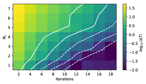
Figure 8: Convergence of dust temperature values for models of different refinement. The colour scale shows the difference of the average dust temperature at the highest level of refinement ($L$=$n_{\rm L}$) compared to the solution after 20 iterations. The number of hierarchy levels $n_{\rm L}$is on the y-axis. Calculations are done without ALI and without a reference field. The contours are drawn at ${\rm log}_{10}\,a$ for $a$=-1.5, -1.0, -0.5, 0.0, and 0.5.

Figure 9 shows the results for a run with run-time refinement of the model. Calculations start with the root grid only ($n_{\rm L}$=1). One level is added on iterations 5, 9, and 15, thereafter the remaining run proceeds with the full $n_{\rm L}$=4 model. When the grid is refined, also the number of photon packages is quadrupled so that the final iterations have the same 18 million photon packages per frequency as in previous tests (e.g. Fig. 4).

The initial iterations are very fast. However, Fig. 9 shows that run-time refinement does not have a significant effect on the final convergence. After the final refinement, the error $|\Delta T|$ is half of the value of the basic run that corresponds to the same run time. However, subsequent convergence remains almost identical to the case where the $n_{\rm L}$$=4$ grid was used on all iterations.

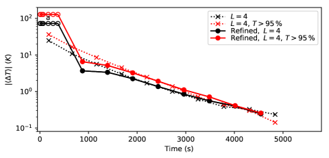
Figure 9: Convergence of temperatures for basic runs with the $n_{\rm L}$$=4$ model(dashed lines) and with run-time refinement of the spatial grid from $n_{\rm L}$$=1$ to $n_{\rm L}$$=4$ (solid lines). The results are shown for the average of all $L=4$ cells (black lines) and for the average of 5% of the warmest $L=4$ cells (red lines). Convergence $|\Delta T|$ is measured as the difference to a run with 40 iterations and the same $n_{\rm P}$. In the case of run-time refinement, the open symbols corresponds to initial iterations with $n_{\rm L}$$<4$, are drawn at $|\Delta T|=100$ K, and only indicate the run times of those steps.

3.6 Variable number of photon packages

Apart from the number of cells, the number of photon packages is the main factor determining the run times. Therefore, we investigated if a good solution can be found faster if the number of packages was increased during the iterations. An acceptable solution clearly requires both convergence and low random errors. Figure 6 already suggested that these are not independent and systematic error measured by $\Delta T$ also depend on the random Monte Carlo noise.

In Fig. 10 we examine runs with 22 iterations where the final number of photon packages $n_{\rm P}$  is again 18 million. However, this time the initial number of photon packages is smaller by a factor of 200 and photon numbers are increased so that $log\,n_{\rm P}$ grows linearly over the iterations.

For the basic method and the reference field method the rate of convergence is similar but the final rms error of the reference field method is two times lower. In principle, if $n_{\rm P}$  were constant, the reference field method could result in an rms noise that is smaller by a factor of $N_{\rm I}^{-1/2}$. The advantage is here smaller because initial iterations employ a smaller number of photon packages. More importantly, the reference field is less efficient because the dust temperatures change significantly over the iterations.

Unlike for example in Fig. 6, the use of ALI not only increases the rms errors but also results in a slower convergence. This is probably a result of large Monte Carlo noise on the initial iterations that also renders the ALI updates noisy and thus ineffective. The combination of ALI and a reference field fairs somewhat better but the convergence measured against the run time is still worse than without ALI. For reference, Fig. Fig. 6 also shows the result for the combination of ALI and a reference field when all iterations use 18 million photon packages. There the convergence per iteration is much faster. When measured against the actual run time, the convergence in $|\Delta T|$ is initially similar and later inferior to the variable $|n_{\rm P}|$ runs.

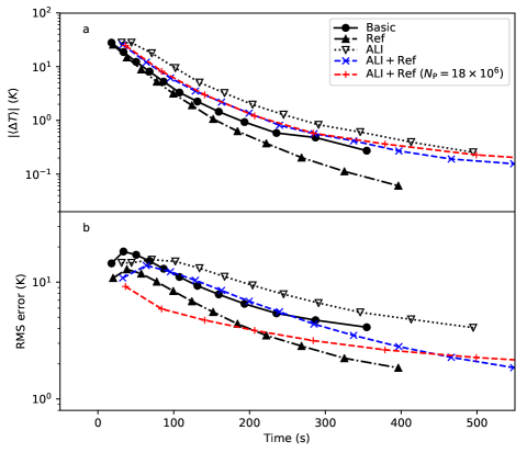
Figure 10: Convergence and rms errors of temperatures in runs where the number of photon packages $n_{\rm P}$  is increased by a factor of 200 over the iterations. The final iterations use 18 million photon packages per frequency. Results are shown for different combinations of ALI and reference field methods, as indicated in frame a. For reference, the red curves show the results for the constant $n_{\rm P}$  of 18 million photon packages per iteration. Markers are drawn for every second iteration.

4 Discussion

In this paper, we have described the implementation of the radiative transfer programme SOC and quantified its performance in the modelling of dust emission from interstellar clouds. Unlike most benchmark papers, we also examined the actual run times and especially the relative performance of CPUs and GPUs.

4.1 Radiative transfer methods

SOC is based on Monte Carlo simulations and the tests showed that it behaved according to expectations. The Monte Carlo noise is inversely proportional to the square root of the number of photon packages. Similarly, the noise is dependent on the level of the grid refinement, each additional hierarchy level approximately decreasing the number of photon package hits by a factor of four and increasing the rms noise by a factor of two. The experiments with photon package splitting schemes were mentioned in this paper only briefly because their success was found to be limited. They do decrease somewhat the noise at higher refinement levels and might be indispensable for deeper hierarchies. However, in our tests there were no significant savings in the actual computational cost. These methods need to be investigated further. The penetration of external radiation into high-density regions is decreased by backscattering and, therefore, photon splitting might need to be combined with directional weighting to increase the probability of photon packages reaching the highest column density regions.

In addition to the pure radiation field simulations, we studied the convergence of the dust temperatures in optically thick models with internal heating sources. The ALI and reference field methods were tested, also in relation to the other run parameters like the number of photon packages per iteration and the discretisation of the model volume.

ALI improves the temperature convergence but is relevant only when both optical depths and dust temperatures are high. In the context of interstellar clouds, benefits are noticeable only near embedded heating sources, potentially in a very small fraction of the whole model volume (although in relative terms a larger fraction of grid cells). To reduce memory requirements (one additional number per cell) and run times, the use of ALI could be restricted to selected cells. This would be only a small complication in the RT implementation. However, in our tests where ALI was included for all cells, the run time overhead was not very significant, only some tens of percent.

The most straightforward way to speed calculations is to use fewer photon packages. This will of course increase the noise of the solution but, when solution also requires a number of iterations, gives room for further optimisations. Significant savings are possible if initial iterations are done fast, with low number of photon packages $n_{\rm P}$. Parameter $n_{\rm P}$  can be increased with iterations, to keep random errors comparable to the convergence errors. This turned out to work less reliably in connection with ALI, which provided clear acceleration only when the random errors were kept low. The final rms error of the solution also tended to be larger when ALI was used (Figs. 7,  10).

The most robust way to speed-up computations was to gradually increase $n_{\rm P}$, without ALI but using the reference field method (Fig. 10). Without a reference field, the final accuracy will be limited by the number of photon packages per iteration (clearly demonstrated by Fig. 6). This determines the rms errors but may also impact the convergence. With a reference field, the rms errors decrease as iterations progress, making it also easier to track the convergence. The fastest convergence in terms of the run time was reached when the number of photon packages $n_{\rm P}$  is increased with iterations. Changes in $n_{\rm P}$  must of course be taken into account also in the reference field updates. Initial iterations are thus given a smaller weight, which is also useful because the reference field is still far from the final solution.

ALI methods are very likely still necessary for models more optically thick than the ones tested in this paper. The critical quantity is the optical depth of individual cells, especially if the ALI scheme does not explicitly consider longer-distance interactions. In general, hierarchical grids enable finer discretisation of dense regions, which reduces the optical depth of individual cells and thus reduces benefits of using ALI. In this paper, only the diagonal part of the $\Lambda$ operator was separated. The next step, explicit treatment of the radiative couplings between a cell and its six Cartesian neighbours, may already be excluded by the associated storage overhead. The implementation in connection with a hierarchical grid would also be significantly more complicated.

Finally, we also tested runs where the spatial discretisation was refined during the iterations. A large cell size used on the first iterations could increase the speed with which information traverses an optically thick model, especially if ALI is used to accelerate the convergence within the individual cells. In practice, the results were not very encouraging (Fig. 9). Iterations with low $n_{\rm L}$are indeed very fast but changes in the gridding cause large temperature jumps and the final convergence is not improved. In the tested model, the temperature field contains significant structure even at very small scales. A change in discretisation significantly changes the radiative transfer problem itself (cf. Fig. 2), also changing the optical depths between the radiation sources and the cells. Our implementation of the re-gridding procedure could be improved. We assigned the temperature of a parent cell to all its children while 3D interpolated values should work better. In smooth models with small density and radiation field gradients, the convergence would naturally be less disturbed by changes in the grid.

We tested SOC using calculations with a single dust population and assuming that the grains are at an equilibrium temperature. SOC will be developed further to allow the modelling of multiple dust components. This requires only small kernel modifications but implies an increase in the memory usage. If the scattering function was constant, one could store for each cell (instead of one number, the density) both the absorption and scattering cross sections. However, to model the scattering accurately, the abundance of each dust population is needed separately for each cell. This makes it possible to make run-time Monte Carlo sampling from the ensemble of scattering functions. However, this will also at least double the memory usage.

Full radiative transfer modelling of dust emission requires both the evaluation of the radiation field and the estimation of the resulting dust emission. When grains are assumed to remain at an equilibrium temperature, the latter problem is not significant for the overall computational cost. However, to model mid-infrared emission from stochastically heated grains, the run times may become dominated by this task, which includes the computation of temperature probability density distributions for each cell, grain population, and grain size. SOC delegates this to an external program. However, in Appendix A we discuss how also these calculations can be sped up by using GPU computing. The use GPUs in this context was already discussed, for example, in Siebenmorgen & Heymann (2012).

4.2 Implementation and CPU vs. GPU comparisons

The current SOC version is implemented in Python that is convenient for rapid development but, as an interpreted language, is not expected to be fast. In practice, this is not a problem because most calculations are performed by the OpenCL kernels that are compiled at run time. In CPU runs with 3D models ($n_{\rm L}$=2), some 93% of the total run time was used by the kernel for the radiative transfer simulation, less than 1% by the dust temperature calculations, and some 2.5% by the kernel for the map calculations. The remaining part includes the execution of the Python host code, the compilation of the OpenCL kernels, the data transfer between the host and the device, and the reading and writing of data files. In CPU runs these thus amount to little more than 3% of the total run time but, because of the much faster kernel execution, can in short GPU runs reach 30%. However, this would not disappear entirely even if the host code were compiled. Indeed, comparisons with previous SOC versions, where the main program was written in C++, suggested at most $\sim$10% overhead due to the use of Python.

Experience has shown that SOC is usually (but not always) slightly faster than CRT (Juvela 2005), when both are run using CPUs and the same non-hierarchical grids. In CRT the critical parts have been parallelised using OpenMP. However, comparisons are not trivial because of slight differences in the implementations (e.g., how randomness is reduced in case of different radiation sources or how the run times scale with the model size). Such tests would be useful, but only when conducted systematically over a large number of test cases and comparing the actual noise properties of the results.

Theoretical peak performance of modern GPUs is very high, which could translate to much shorter run times and smaller energy consumption (Huang et al. 2009; Said et al. 2016). In the test system the theoretical ratio was over a factor of 20 in favour of the GPU. In practice the theoretical speed-up is never reached, mainly because of data transfer overheads. This was true also in the SOC tests where the GPU was typically faster only by a factor of 2-10.

The relative performance of GPUs tends to improve with increasing problem sizes, with increasing number of cells or, as in Fig. 2, with increasing number of photon packages. However, there were also exceptions. In the case of point source simulations (Fig. 2c), this could be caused by the increasing overheads in GPU atomic operations when many threads are simultaneously updating a small number of cells close to the source. The same explanation may also apply to the problems seen when using emission weighting on GPUs. Although emission weighting results in lower noise for a given $n_{\rm P}$, on GPU it increased (at $n_{\rm P}$$\sim 10^{6}$) the run times by up to a factor of a few (Fig. 3c). Also in this case, most updates concern a small number of cells, those with the highest dust temperatures. The effect is accentuated by high optical depths that result in frequent scatterings and thus even more frequent updates. These effects will be smaller for models with multiple point sources, larger number of cells, and lower optical depths. The problem could be alleviated by interleaving the creation and tracking of photon packages so that all threads would not create new photon packages in the same cells and at exactly the same time. New OpenCL versions with native support for atomic operations should further decrease the overheads. In Fig. 3c, the problem disappears for large $n_{\rm P}$  but this is only a side effect from the limit on the maximum number of photon packages emitted from any single cell.

In contrast with the GPU results, on CPU the calculations were faster when emission weighting was used. This could result from better cache utilisation, similar to the factor of $\sim$2 effect observed in Lunttila & Juvela (2012). In OpenCL, the threads belonging to the same work group perform computations in lockstep. All threads thus create and perform initial tracking of photon packages at the same time and within a small volume around the embedded radiation source. With a smaller number of threads and larger cache memories, the net effect can be positive on CPUs. The data for the most frequently accessed cells may remain in cache during a whole run, but it is difficult to say if this alone explains the observed factor of $\sim$5 speed up (Fig. 3c). The above examples at least demonstrate that, although the same program can be run on both CPUs and GPUs, best performance may require different algorithm optimisations on different platforms.

5 Conclusions

The ability of SOC to produce correct results in dust radiative transfer problems was already tested in Gordon et al. (2017). In this paper, we concentrated on the performance of SOC and investigated methods that could speed up the computations in problems where the final dust temperatures are obtained only after several iterations. The tests resulted in the following conclusions:

• SOC performs well in comparison to e.g. the CRT program (Juvela 2005) and modern GPUs provide a factor of 2–10 speed-up over a multicore CPU. Further reduction of run times should be possible by fine-tuning the algorithms.

• The noise of the temperature solution behaves as expected: it is inversely proportional to the square root of photon packages and increases by a factor of two for each additional level of the spatial grid hierarchy. The tested photon splitting scheme did not significantly reduce the noise of high hierarchy levels relative to the run time.

• In the test cases, ALI provided moderate acceleration for the convergence of dust temperature values. The run time overhead varied from case to case but was of the order of 10%, small compared to the potential benefits from the faster convergence.

• The use of a reference field without ALI was found to be the most robust alternative. The desired accuracy could be reached in the least amount of time by doing the initial iterations with fewer photon packages.

SOC will be developed further to accommodate multiple dust populations and in Appendix A we already discuss tests on the use of GPUs to speed up to the calculations of stochastically heated grain emission.

Appendix A Calculations with stochastically heated grains

SOC concentrates on solving the radiative transfer problem and only solves grain temperatures for grains in equilibrium with the radiation field. For stochastically heated grains, these computations are delegated to an external program, such as the one that in Camps et al. (2015) was used in connection with the CRT code. We report here some results from tests on implementing similar routines with Python and OpenCL. We refer to the old code as the C program and the new one as the OpenCL program.

Tests were made using a single dust component and a three-dimensional model cloud that consisted of 8000 cells, sufficient to get accurate run-time measurements. The dust corresponds to astronomical silicates as defined in the DustEM package Compiègne et al. (2011). The grain size distribution extends from 4 nm to 2 $\mu$m is discretised into 25 logarithmic size bins. All grains were treated in the tests as stochastically heated while in real applications the largest grains could be handled using the equilibrium temperature approximation. The calculations employed a logarithmic discretisation of enthalpies that in temperature extend from 4 K to 150 K for the largest and from 4 K to 2500 K for the smallest grains. The model cloud is illuminated by the standard interstellar radiation field (Mathis et al. 1983). The column density of the cloud varies from $N({\rm H}_{2})\sim 3\times 10^{19}\, {\rm cm}^{-2}$ to $N({\rm H}_{2})=1\times 10^{22}\, {\rm cm}^{-2}$. This ensures a wide range of radiation field intensities, especially for the shorter wavelengths that are relevant for mid-infrared dust emission. Radiative transfer simulations used a logarithmic grid of 128 frequencies between the Lyman limit and 2 mm.

We used as the reference the C program and its routine that solves the dust temperatures under the “thermal continuous” cooling approximation as described in Draine & Li (2001). The calculation reduces to a linear set of equations where the unknowns are the fraction of dust in each enthalpy bin. The C program pre-calculates weights for the integration of the absorbed energy over frequency as well as the cooling rates that in the thermal continuous approximation only extend downwards to the next enthalpy bin. When the dust emission is solved cell-by-cell, the program gets a vector of radiation field intensities (in practice number of absorbed photons). In the transition matrix $R$, the upward transitions ($R_{j,i}$, $i<j$) are obtained by taking a vector product of the intensity with the integration weights. The pre-calculated cooling rates occupy the elements $R_{i-1,i}$ above the main diagonal. The diagonal elements $R_{i,i}$ are determined from detailed balance and are equal to the sum of the other column elements multiplied by minus one. The matrix elements $R_{j,i}=0$, $i>j$ are zeros, which means that the linear equations can be solved efficiently with forward-substitutions. The C program is parallelised with OpenMP, further optimisations including the use of SSE instructions.

In the OpenCL programme we tested first the use of an iterative solver. Iterative solvers are attractive because one is typically dealing with large 3D models where the neighbouring cells are subjected to a very similar radiation field. By using the solution of the preceding cell as the starting values for the next one, it is likely that the number of iterations can be kept small. We tested only basic Gauss-Seidel iterations with Jacobi (diagonal) preconditioning. By using the solution of the first cell to start the iterations for each of the other cells, less than ten iterations and a maximum of $\sim$50 were needed to reach an accuracy that in the final surface brightness maps translated to rms errors of a couple of per cent (over a spectral range spanning more than 10 orders of magnitude in absolute intensity). On the CPU, using the same number of CPU cores, the run time was nearly identical to that of the C program. On a GPU, the OpenCL version was faster by a factor of $\sim$5. In the case of the thermal continuous approximation, the explicit solution is already very fast. Therefore, in a general case ($R_{j,i}\neq 0$ for $j<i$), iterative solvers should be a good option.

We could not exactly reproduce the results of the C program even with more iterations. This may be due to the use single-precision floating point numbers. The use of double precision would slow down the GPU computations, depending on the hardware. Furthermore, although Gauss-Seidel iterations provided a sufficient (but still a low-precision) solution in just a few iterations, the convergence is not guaranteed. The rate matrix is not diagonally dominant and the spectral radius of the iteration matrix was either very close to or even larger than one. The iterations should thus eventually diverge, which was indeed observed if continued further beyond one hundred iterations. However, when the problem is similar for a very large number of cells, one could calculate better preconditioners with a small per-cell cost.

We also implemented an explicit forward-substitution algorithm similar to that of the C programme. This is the natural option in the case of the thermal continuous approximation. The routine worked reliably but only when part of the operations were performed in double precision. The use of double precision resulted in some 25% increase in the GPU run times but had no effect on CPUs. The results were identical to the C program, almost down to the machine precision. Because the algorithm is faster, the run times were shorter than for the iterative solver. Compared to the C programme, the OpenCL routine was 5.6 times faster when run on CPU and 21 times faster when run on GPU. The speed-up on the CPU suggests that the parallelisation of the C programme was not optimal but the results also depend on other factors, such as the memory and disk access patterns. On the laptop, the OpenCL program ran $\sim$4 times faster on the GPU than on the six-core CPU.

The actual wall-clock run time on the laptop GPU was some 0.5 ms per cell, which includes the calculations of the dust temperature distributions and the resulting dust emission at 128 frequencies. Assuming that modelling involved four dust populations, this would translate to a rate of 500 cells per second and a run time of some half an hour for a model of $10^{6}$ cells. The time required for the radiative transfer simulations is of the same order of magnitude, the exact balance depending on the chosen frequency, enthalpy, and grain size discretisations. The costs of radiative transfer and dust temperature calculations both also scale approximately linearly with the number of cells. It is therefore already feasible to directly solve the emission of stochastically heated grains even for relatively large 3D models. Table look-up methods are still relevant because they also reduce number of frequencies at which the radiation field needs to be estimated (Juvela & Padoan 2003; Baes et al. 2011). Nevertheless, GPUs can speed up the construction of large look-up tables and thus improve the accuracy of also those methods.

Appendix B Examples of surface brightness maps

In Sect. 3 we examined the accuracy of SOC results mainly in terms of dust temperature. Here we present examples of surface brightness maps that correspond to the tests in Figs. 6 and  7, the final result after 20 iterations. Surface brightness errors are shown by plotting the difference of two independent runs.

Figure 11 shows the maps that correspond to Fig. 6, the runs without ALI where the number of photon packages per iteration was 18 million or smaller by a factor of 8 or 64. The noise is small enough to be visible only in the difference maps that here only contain errors from the simulation of the re-radiated dust emission. The error maps show a radial pattern because hot dust is found only close to the central point source. The relative contribution of re-radiated dust emission is smaller in directions where more of the point source radiation escapes the central clump. This explains the general asymmetry of the pattern where the errors tend to be smaller on the upper left hand side.

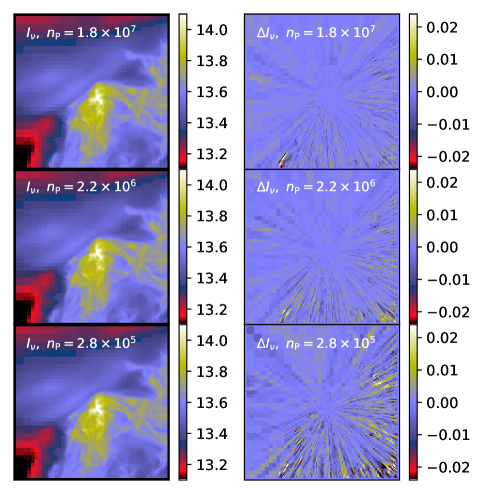
Figure 11: Surface brightness maps at 100 $\mu$m for the final iteration of the non-ALI runs of Fig. 6. The three rows correspond, respectively, to the default $n_{\rm P}$  value of $1.8\times 10^{7}$ and to $n_{\rm P}$  values smaller by a factor of 8 or 64. The left hand frames show the 100 $\mu$m surface brightness $I_{\nu}(100\,\mu{\rm m})$ and the right hand frames the difference $\Delta I_{\nu}(100\,\mu{\rm m})$ between two identical runs. All maps are in units of $10^{8}$ Jy sr^-1.

Figure 12 shows the results when also the reference field technique is used. The upper frames correspond directly to the runs in Fig. 7.

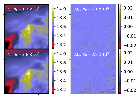
Figure 12: As Fig. 11 but for the runs of Fig. 7 with a reference field. The number of photon packages is $n_{\rm P}$=$1.1\times 10^{6}$ (upper frames) or four time smaller (lower frames). Maps are in units of $10^{8}$ Jy sr^-1.