Surface Crouzeix-Raviart element for the Laplace-Beltrami equation

Abstract

This paper is concerned with the nonconforming finite element discretization of geometric partial differential equations. In specific, we construct a surface Crouzeix-Raviart element on the linear approximated surface, analogous to a flat surface. The optimal error estimations are established even though the presentation of the geometric error. By taking the intrinsic viewpoint of manifolds, we introduce a new superconvergent gradient recovery method for the surface Crouzeix-Raviart element using only the information of discretization surface. The potential of serving as an asymptotically exact a posteriori error estimator is also exploited. A series of benchmark numerical examples are presented to validate the theoretical results and numerically demonstrate the superconvergence of the gradient recovery method.

AMS subject classifications.  Primary 65N30; Secondary 45N08

Key words.  Laplace-Beltrami operator, nonconforming, surface finite element method, Crouzeix-Raviart element, gradient recovery, superconvergence.

1 Introduction

Numerical methods for approximating partial differential equations (PDEs) with solutions defined on surfaces are of growing interests over the last decades. Since the pioneer work of Dziuk [25], there is tremendous development on finite element methods[13, 2, 20, 21, 22, 26, 29, 31, 35, 36, 17]. Fluid equations on manifolds have many important applications in fluidic biomembranes[3, 6], computer graphics[27, 33], geophysics[37, 41]. Typically, numerical simulation of surface Stokes or Navier-Stokes equations is unavoidable. In the literature, there are several works on them, for example, see [28, 39, 38, 7, 34]. It is well known that linear surface element is not a stable pair for surface Stokes equations [12]. One can fix it by adding a stabilizing term[39, 34] or using Taylor-Hood element [28].

In the planar domain case, a simpler way to overcome this difficulty is to use the Crouzeix-Raviart element. The Crouzeix-Raviart element was firstly proposed by Crouzeix and Raviart in [18] to solve a steady Stokes equation. Different from the Courant element, such element is only continuous at edge centers of a triangulation. In that sense, it is a nonconforming element. In addition to being used to construct a simple stable finite element pair for Stoke problems, the method is also proven to be locking free for Lame problems[11]. It can be viewed as a universal element for solids, fluids, and electromagnetic, see the recent review paper [9] and the references therein.

Our first purpose is to extend this exotic nonconforming element to a surface setting. Compared with the counterpart in the flat space, there is an additional geometric error due to the discretization of the surface. One of the main difficulties is to estimate the nonconforming error. The key ingredient of this step is to conduct all the error analysis on the discretized surface instead of on the exact surface. It should be pointed out that, in general, two triangles sharing a common edge are not on the same plane. The standard argument [8, 16] for nonconforming finite element method cannot be applied directly and the nonconforming error is coupled together with the geometric error. By carefully using the geometric approximation properties, we show that the geometric error has no impact on the overall convergence results.

Our second purpose is to propose a superconvergent post-processing technique for the surface Crouzeix-Raviart element. On the planar domain case, there are several post-processing techniques[14, 30] for the Crouzeix-Raviart element. In particular, Guo and Zhang employed a local least-squares fitting procedure at every edge center to generate a more accurate approximate gradient. The most straightforward way of generalizing such idea to a surface setting is to project a local patch onto its tangent plane as in [42]. However, there are two barriers to the surface Crouzeix-Raviart element: first, it requires the exact normal vectors; second, it requires the edge centers located on the exact surface. Those two difficulties can be alleviated by going back to the original definition of the covariant derivative as in [24]. In specific, we firstly adopt a least-squares procedure to recover the local parametric map and then employ another least-squares fitting on the parameter domain. Based on the gradient recovery method, we introduce a recovery-type a posteriori error estimator for the surface Crouzeix-Raviart element.

The rest of the paper is organized as the follows. In section 2, we give a brief introduction to some preliminary knowledge on the tangential derivative and an exemplary model problem. In section 3, we introduce the discretized surface and present the surface Crouzeix-Raviart element. Section 4 is devoted to the analysis of discrete energy error and $L^{2}$ error on the discrete surface. In section 5, we propose a superconvergent post-processing technique. A series of benchmark numerical examples are presented to support our theoretical finding in Section 6. Some conclusions are drawn in Section 7.

2 Preliminary

2.1 Notation

In the paper, we shall consider $\Gamma$ is an oriented, connected, $C^{\infty}$ smooth regular surface in $\mathbb{R}^{3}$ without boundary. The sign distance function of $\Gamma$ is denoted by $d(x)$. Let $\nabla$ be the standard gradient operator in $\mathbb{R}^{3}$. Then the unit outward-pointing normal vector is $n(x)=\nabla d(x)$ and the Weingarten map is $\mathbf{H}(x)=\nabla n(x)=\nabla^{2}d(x)$.

Let $U=\{x\in\mathbb{R}^{3}:\text{dist}(x,\Gamma)\leq\delta\}$ be a strip neighborhood around $\Gamma$ with distance $\delta$ where $\text{dist}(x,\Gamma)$ is the Euclidean distance between $x$ and $\Gamma$. Assume $\delta$ is small enough such that there exists a unique projection $p(x):U\rightarrow\Gamma$ in the form of

$$p(x)=x-d(x)n(p(x)).$$ (2.1)

Let $P=Id-n\otimes n$ be the tangential projection operator where $\otimes$ is the tensor product. The tangential gradient of a scalar function $v$ on $\Gamma$ is defined to be

$$\nabla_{\Gamma}u=P\nabla u=\nabla u-(\nabla u\cdot n)n.$$ (2.2)

For a vector field $w\in\mathbb{R}^{3}$, the tangential divergence is

$$\mbox{div}_{\Gamma}w=\nabla_{\Gamma}\cdot w=\nabla\cdot w-n^{t}\nabla wn$$ (2.3)

The Laplace-Beltrami operator $\Delta_{\Gamma}$ is just the tangential divergence of the tangential gradient, i.e.

$$\Delta_{\Gamma}v=\mbox{div}_{\Gamma}\nabla_{\Gamma}v=\Delta v-(\nabla v\cdot n)(\nabla\cdot n)-n^{t}\nabla^{2}vn.$$ (2.4)

Let $\alpha=(\alpha_{1},\alpha_{2},\alpha_{3})$ be the $3$-index and $|\alpha|=\sum_{i=1}^{3}\alpha_{i}$ with $\alpha_{i}$ being a nonnegative integer. Let $D^{\alpha}_{\Gamma}$ be the $|\alpha|$th order tangential derivative. Assume $\omega$ being a subset of $\Gamma$ and $m$ being a nonnegative integer. The Sobolev space $H^{m}(\omega)$ on $\omega$ [43] is defined as

$$H^{m}(\omega)=\left\{v\in L^{2}(\omega)|D^{\alpha}_{\Gamma}v\in L^{2}(\omega),|\alpha|\leq m\right\},$$ (2.5)

with norm

$$\|v\|_{H^{m}(\omega)}=\left(\sum_{\alpha\leq m}\|D^{\alpha}_{\Gamma}\|^{2}_{L^{2}(\omega)}\right)^{1/2},$$ (2.6)

and semi-norm

$$|v|_{H^{m}(\omega)}=\left(\sum_{\alpha=m}\|D^{\alpha}_{\Gamma}\|^{2}_{L^{2}(\omega)}\right)^{1/2}.$$ (2.7)

Throughout this article, we use $x\lesssim y$ to denote $x\leq Cy$ where the letter $C$ denotes a generic constant which is independent of h and may not be the same at each occurrence.

2.2 Model problem

In this paper, we shall consider the following model Laplace-Beltrami equation

$$-\Delta_{\Gamma}u+u=f,$$ (2.8)

for a given $f\in L^{2}(\Gamma)$.

The variational formulation of (2.8) is to find $u\in H^{1}(\Gamma)$ such that

$$a(u,v)=\ell(v),\quad\forall v\in H^{1}(\Gamma)$$ (2.9)

where

$$a(w,v)=(\nabla_{\Gamma}w,\nabla_{\Gamma}v)+(w,v),$$ (2.10)

and

$$\ell(v)=(f,w),$$ (2.11)

with $(\cdot,\cdot)$ being the standard $L^{2}$ inner product on $\Gamma$. The Lax-Milligram theorem implies (2.9) has a unique solution and there holds the following regularity [4]

$$\|u\|_{H^{2}(\Gamma)}\lesssim\|f\|_{L^{2}(\Gamma)}.$$ (2.12)

3 The nonconforming finite element method

3.1 Approximate surface

Suppose $\Gamma_{h}$ is a polyhedral approximation of $\Gamma$ with planar triangular surface. Let $\mathcal{T}_{h}$ be the associated mesh of $\Gamma_{h}$ and $h=\max_{T\in\mathcal{T}_{h}}\mbox{diam}(T)$ be its maximum diameter. Furthermore, we assume the mesh $\mathcal{T}_{h}$ is sharp regular and quasi-uniform triangulation [8, 10, 16] and all vertices lie on $\Gamma$. Let $\mathcal{E}_{h}$ be the set of all edges of triangular faces in $\mathcal{T}_{h}$. For any edge $E\in\mathcal{E}_{h}$, let $m_{E}$ be the middle point of edge $E$. The set of all edge middle points of $\mathcal{T}_{h}$ is denoted by $\mathcal{M}_{h}$. For any $T\in\mathcal{T}_{h}$. let $n_{h}$ be the unit outer normal vector to $\Gamma_{h}$ on $T$. The projection onto the tangent space of $\Gamma_{h}$ can be defined

$$P_{h}=Id-n_{h}\otimes n_{h}.$$ (3.13)

Similarly, for a scalar function $v$ on $\Gamma_{h}$, we can define its tangential gradient as

$$\nabla_{\Gamma_{h}}v=P_{h}\nabla v,$$ (3.14)

and the Laplace-Beltrami operator on $\Gamma_{h}$ as

$$\Delta_{\Gamma_{h}}v=\nabla_{\Gamma_{h}}\cdot\nabla_{\Gamma_{h}}v_{h}$$ (3.15)

Recall that $p(x)$ is a projection map from $U$ to $\Gamma$. For any $T\in\mathcal{T}_{h}$, let $T^{l}=p(T)$ be the curved triangular face on $\Gamma$. Denote the set of all curved triangular faces by $\mathcal{T}_{h}^{l}$ , i.e. $\mathcal{T}_{h}^{l}=\left\{T^{l}:T\in\mathcal{T}_{h}\right\}$. Then $\mathcal{T}_{h}^{l}$ forms a conforming triangulation of $\Gamma$ such that

$$\Gamma=\bigcup_{T^{l}\in\mathcal{T}_{h}^{l}}T^{l}.$$ (3.16)

For any edge $E\in\mathcal{E}_{h}$, there exists two triangles $T^{+}$ and $T^{-}$ such that $E=\partial T^{+}\cap\partial T^{-}$. The projection on $T^{+}$ and $T^{-}$ are denoted by $P_{h}^{+}$ and $P_{h}^{-}$. Also, we use the notation $\nabla_{\Gamma_{h}}^{+}=P_{h}^{+}\nabla$ to denote the tangent gradient in $T^{+}$. Similar notation is adopted in $T^{-}$. The conormal of $E$ to $T^{+}$, which is denoted by $n_{E}^{+}$, is the unit outward vector of $E$ in the tangent plane of $T$ . Similarly, let $n_{E}^{-}$ be the conormal of $E$ to $T^{-}$. Analogously, on the curved edge $E^{l}=p(E)$, we denote its conormals by $n_{E^{l}}^{\pm}$. Note that $n_{E^{l}}^{+}=-n_{E^{l}}^{-}$. The unit outer normals of $\Gamma_{h}$ on $T^{+}$ and $T^{-}$ are denoted by $n_{h}^{+}$ and $n_{h}^{-}$, respectively. Then it easy see that $n_{h}^{+}\perp n_{E}^{+}$ and $n_{h}^{-}\perp n_{E}^{-}$. We define the jump of a function $v_{h}$ across $E$ by

$$\llbracket v\rrbracket=\lim_{s\rightarrow 0_{+}}\left(v(x-sn_{E}^{+})-v(x-sn_{E}^{-})\right).$$ (3.17)

3.2 The surface Crouzeix-Raviart finite element method

The surface Crouzeix-Raviart finite element space on $\mathcal{T}_{h}$ is defined to be

$$V_{h}=\left\{v_{h}\in L^{2}(\Gamma_{h}):v_{h}|_{T}\in\mathbb{P}^{1}(T)\text{ and }v_{h}\text{ is continuous at }\mathcal{M}_{h}\right\},$$ (3.18)

where $\mathbb{P}_{1}(T)$ is the set of linear polynomials on $T$. By the definition of jump (3.17) and the midpoint rule, a piecewise linear function $v$ is in $V_{h}$ if and only if

$$\int_{E}\llbracket v\rrbracket d\sigma_{h}=0.$$ (3.19)

To simplify the notation, we firstly define a discrete bilinear form $a_{h}(\cdot,\cdot)$ on $V_{h}\times V_{h}$ as

$$a_{h}(w_{v},v_{h})=\sum_{T\in\mathcal{T}_{h}}\int_{T}\nabla_{\Gamma_{h}}w_{h}\cdot\nabla_{\Gamma_{h}}w_{h}\cdot ds_{h}+(w_{h},v_{h})_{\Gamma_{h}}$$ (3.20)

and a linear functional $\ell_{h}(\cdot)$ on $V_{h}$ as

$$\ell_{h}(v_{h})=(f\circ p,v_{h})_{\Gamma_{h}}$$ (3.21)

where $(\cdot,\cdot)_{\Gamma_{h}}$ is the standard $L^{2}$ inner product of $L^{2}(\Gamma_{h})$. Then the surface Crouzeix-Raviart finite element discretization of the model problem (2.8) reads as: find $u_{h}\in V_{h}$ such that

$$a_{h}(u_{h},v_{h})=\ell_{h}(v_{h}),\quad\forall v_{h}\in V_{h}.$$ (3.22)

We define an broken $H_{1}$ semi-norm on $V_{h}$ as

$$|v_{h}|_{H^{1}(\Gamma_{h};\mathcal{T}_{h})}^{2}=\sum_{T\in\mathcal{T}_{h}}\|\nabla_{\Gamma_{h}}v_{h}\|_{L^{2}(T)}^{2}$$ (3.23)

The corresponding discrete energy norm is given by

$$\|v\|_{h}^{2}=|v_{h}|_{H^{1}(\Gamma_{h};\mathcal{T}_{h})}^{2}+\|v_{h}\|_{L^{2}(\Gamma_{h})}^{2}=a_{h}(v_{h},v_{h}).$$ (3.24)

Then, it is easy to show that following Lemma:

Lemma 1.

$\|v\|_{h}$ is a norm on $V_{h}$. The Lax-Milgram theorem implies the discrete variational problem (3.22) admits a unique solution.

4 A priori error estimates

4.1 Lift and extension functions

To compare the error between the exact solution $u$ defined on $\Gamma$ and the finite element solution $u_{h}$ defined on $\Gamma_{h}$, we need to establish connections between the functions defined on $\Gamma$ and $\Gamma_{h}$.

Following the notation as in [13], for a function $v$ defined on $\Gamma$, we extend it to $U$ and define the extension $v^{e}$ by

$$v^{e}(x)=v(p(x)),\quad\forall x\in U.$$ (4.25)

Similarly, for a function $v_{h}$ defined on $\Gamma_{h}$, we define the lift of $v_{h}$ onto $\Gamma$ by

$$v^{l}(x)=v(\xi(x)),\quad\forall x\in\Gamma,$$ (4.26)

where $\xi(x)$ is the unique solution of

$$x=p(\xi)=\xi-d(\xi)n(x).$$ (4.27)

Then we build the relationship in gradients of extensions and lifts. For such propose, we introduce the matrix $B=P(x)-d(x)H(x)$. It is easy to check that $B=PB=BP=PBP$. The following relationship is proved in [13, 22, 31]

$$\nabla_{\Gamma_{h}}v^{e}=P_{h}B(\nabla_{\Gamma}v)^{e}.$$ (4.28)

Let $ds$ and $ds_{h}$ be the surface measures of $\Gamma$ and $\Gamma_{h}$. For any $x\in\Gamma_{h}$, [22] shows that there exists $\mu_{h}$ such that $ds\circ p(x)=\mu_{h}(x)ds_{h}(x)$ with

$$\mu_{h}(x)=(1-d(x)k_{1}(x))(1-d(x)k_{2}(x))n\cdot n_{h}.$$ (4.29)

Throughout the paper, we assume that $\Gamma_{h}\subset U$. In the following, we collect some geometric approximation results which will be used in our proof:

Lemma 2.

Suppose $\Gamma_{h}\subset U$ is a polyhedral approximation of $\Gamma$. Assume the mesh size $h$ is small enough. Then the following error estimates hold:

$$\|d\|_{L^{\infty}(T)} \lesssim h^{2},$$ (4.30)

$$\|1-\mu_{h}\|_{L^{\infty}(T)} \lesssim h^{2},$$ (4.31)

$$\|n-n_{h}\|_{L^{\infty}(T)} \lesssim h,$$ (4.32)

$$\|P-P_{h}\|_{L^{\infty}(T)} \lesssim h,$$ (4.33)

$$\|n_{E^{l}}^{+/-}-Pn_{E}^{+/-}\|_{L^{\infty}(T)} \lesssim h^{2},$$ (4.34)

$$\|\Delta_{\Gamma_{h}}u^{e}-(\Delta_{\Gamma}u)^{e}\|_{L^{2}(T)} \lesssim h\|u\|_{H^{2}(T^{l})},$$ (4.35)

where $|\cdot|$ is the standard Euclidean norm.

Proof.

The inequalities (4.30)–(4.33) can be proved using the standard linear interpolation theory. Their proof can be found in [22]. The last two estimates were proved in [31]. ∎

Remark 4.1.

For the planar domain case, it is well known that $n_{E}^{+}=-n_{E}^{-}$ and hence $|n_{E}^{+}+n_{E}^{-}|=0$. But this relationship does not hold any more in the surface setting.

To connect the function defined on the exact surface and its extension on the discrete surface, we need the following norm equivalence theorem whose proof can be proved in [25, 31]

Lemma 3.

Let $T\in\mathcal{T}_{h}$. If $v\in H^{2}(T)$, then the following results hold:

$$\|v^{l}\|_{L^{2}(T^{l})}\lesssim \|v\|_{L^{2}(T)}\lesssim\|v^{l}\|_{L^{2}(T^{l})},$$ (4.36)

$$|v^{l}|_{H^{1}(T^{l})}\lesssim |v|_{H^{1}(T)}\lesssim|v^{l}|_{H^{1}(T^{l})},$$ (4.37)

$$|v|_{H^{2}(T)}\lesssim\|v^{l}\|_{H^{2}(T^{l})},$$ (4.38)

$$|v^{l}|_{H^{2}(T^{l})}\lesssim \|v\|_{H^{2}(T)}.$$ (4.39)

Also, we need the following norm equivalence results for function defined on the edge of an element [13]

Lemma 4.

Let $E\in\mathcal{E}_{h}$. If $v\in H^{1}(E)$, then the following results hold:

$$\|v^{l}\|_{L^{2}(E^{l})}\lesssim \|v\|_{L^{2}(E)}\lesssim\|v^{l}\|_{L^{2}(E^{l})},$$ (4.40)

$$|v^{l}|_{H^{1}(E^{l})}\lesssim |v|_{H^{1}(E)}\lesssim|v^{l}|_{H^{1}(E^{l})}.$$ (4.41)

4.2 The nonconforming interpolation

For any $T\in\mathcal{T}_{h}$, let $\mathcal{E}_{T}$ be the set of three edges of $T$. We define the local interpolation operator $\Pi_{T}:H^{1}(T)\rightarrow\mathbb{P}_{1}(T)$ by

$$(\Pi_{T}v)(m_{E})=\frac{1}{|E|}\int_{E}vd\sigma_{h},\quad\forall v\in H^{1}(T),\,E\in\mathcal{E}_{T},$$ (4.42)

where $|E|$ is the length of $E$. By the midpoint rue, we can show that

$$\int_{E}(\Pi_{T}v)d\sigma_{h}=\int_{E}vd\sigma_{h},\quad E\in\mathcal{E}_{T}.$$ (4.43)

Let $h_{T}$ be the diameter of $T$. Then the following error estimate holds [18, 9]

$$\|v-\Pi v\|_{L^{2}(T)}+h_{T}|v-\Pi v|_{H^{1}(T)}\lesssim h_{T}^{2}|v|_{H^{2}(T)},$$ (4.44)

for any $v\in H^{2}(T)$. The global interpolation operator $\Pi_{h}:H^{1}(\Gamma_{h})\rightarrow V_{h}$ is defined by

$$(\Pi_{h}v)|_{T}=\Pi_{T}v,\quad\forall T\in\mathcal{T}_{h}.$$ (4.45)

It follows from (4.44) that

$$\|v-\Pi_{h}v\|_{L^{2}(\Gamma_{h})}+h|v-\Pi_{h}v|_{H^{1}(\Gamma_{h};\mathcal{T}_{h})}\lesssim h^{2}|v|_{H^{2}(\Gamma_{h})},$$ (4.46)

In particular, let $v=u^{e}$. Then we have

$$\inf_{v_{h}\in V_{h}}\|u^{e}-v_{h}\|_{h}\leq|v-\Pi_{h}v|_{H^{1}(\Gamma_{h};\mathcal{T}_{h})}+\|u-\Pi_{h}u^{e}\|_{L^{2}(\Gamma_{h})}\lesssim h|u^{e}|_{H^{2}(\Gamma_{h})}.$$ (4.47)

4.3 Energy error estimate

In this subsection, we establish the error bound in the discrete energy error. Our main tool of the error estimation is the second Strang Lemma [16, 10, 8]:

Lemma 5 (The second Strang Lemma).

Suppose $u$ is the exact solution of (2.9) and $u_{h}$ is the finite element solution of (3.22) . Then we obtain that

$$\begin{split}||u^{e}-u_{h}||_{h}\lesssim&\inf_{v_{h}\in V_{h}}\|u^{e}-v_{h}\|_{h}+\sup_{w_{h}\in V_{h}}\frac{|a_{h}(u^{e},w_{h})-(f^{e},w_{h})|}{\|w_{h}\|_{h}}\end{split}$$ (4.48)

Remark 4.2.

We also call the first term is the approximation error and the second term is the nonconforming consistency error. But different from the planar domain case, the second term also involves the geometric error in addition to the classical nonconforming consistency error. We measure the error using the discrete energy norm on the approximate surface and this is the key part to bound the nonconforming consistency error.

We prepare the energy error estimation with some geometric error estimates. We begin with the following Lemma:

Lemma 6.

Let $u$ be the solution of (2.9) and $u^{e}$ be its extension to $U$ defined by (4.25). Then we have the following error estimates holds

$$|(u,w_{h}^{l})-(u^{e},w_{h})_{\Gamma_{h}}|\lesssim h^{2}\|u\|_{L^{2}(\Gamma)}\|w_{h}\|_{L^{2}(\Gamma_{h})},$$ (4.49)

$$|(f,w_{h}^{l})-(f^{e},w_{h})_{\Gamma_{h}}|\lesssim h^{2}\|f\|_{L^{2}(\Gamma)}\|w_{h}\|_{L^{2}(\Gamma_{h})}.$$ (4.50)

for any $w_{h}\in V_{h}$.

Proof.

We only prove (4.50) and (4.49) can be proved similarly. Applying the change of variable, we have

$$\begin{split}|(f,w_{h}^{l})-(f^{e},w_{h})_{\Gamma_{h}}|\lesssim|((\mu_{h}-1)f^{e},w_{h})_{\Gamma_{h}}\lesssim h^{2}\|f^{e}\|_{L^{2}(\Gamma_{h})}\|w_{h}\|_{L^{2}(\Gamma_{h})}\end{split}$$

where we have used the error estimate (4.31). ∎

Next, we prove a lemma for estimate the error involving two conomorals of an edge.

Lemma 7.

Let $u$ be the solution of (2.9) and $u^{e}$ be its extension to $U$ defined by (4.25). Then we have the following error estimates holds

$$\sum_{E\in\mathcal{E}_{h}}\int_{E}\left(n_{E}^{+}\cdot\nabla_{\Gamma_{h}}^{+}u^{e}+n_{E}^{-}\cdot\nabla_{\Gamma_{h}}^{-}u^{e}\right)^{2}d\sigma_{h}\leq h^{3}\|u\|^{2}_{H^{2}(\Gamma)}.$$ (4.51)

Proof.

Using the triangle inequality and (4.28), we have

$$\begin{split}&\int_{E}\left(n_{E}^{+}\cdot\nabla_{\Gamma_{h}}^{+}u^{e}+n_{E}^{-}\cdot\nabla_{\Gamma_{h}}^{-}u^{e}\right)^{2}d\sigma_{h}\\ =&\int_{E}\left(n_{E}^{+}\cdot P_{h}^{+}B(\nabla_{\Gamma}u)^{e}+n_{E}^{-}\cdot P_{h}^{-}B(\nabla_{\Gamma}u)^{e}\right)^{2}d\sigma_{h}\\ =&\int_{E}\left(Pn_{E}^{+}\cdot B(\nabla_{\Gamma}u)^{e}+Pn_{E}^{-}\cdot B(\nabla_{\Gamma}u)^{e}\right)^{2}d\sigma_{h}\\ \lesssim&\int_{E}\left((Pn_{E}^{+}-n_{E^{l}}^{+})\cdot B(\nabla_{\Gamma}u)^{e}\right)^{2}d\sigma_{h}+\\ &\int_{E}\left((n_{E^{l}}^{-}-Pn_{E}^{-})\cdot B(\nabla_{\Gamma}u)^{e}\right)^{2}d\sigma_{h}\\ \lesssim&h^{4}\int_{E}\left|(\nabla_{\Gamma}u)^{e}\right|^{2}d\sigma_{h}\\ \lesssim&h^{4}\int_{E^{l}}\left|\nabla_{\Gamma}u\right|^{2}d\sigma,\end{split}$$ (4.52)

where we have used (4.34) in the second inequality and norm equivalence (4.41) in the last inequality.

Summing over over all $E\in\mathcal{E}_{h}$ and applying the trace inequality, we have

$$\begin{split}&\sum_{E\in\mathcal{E}_{h}}\int_{E}\left(n_{E}^{+}\cdot\nabla_{\Gamma_{h}}^{+}u^{e}+n_{E}^{-}\cdot\nabla_{\Gamma_{h}}^{-}u^{e}\right)^{2}d\sigma_{h}\\ \lesssim&h^{4}\sum_{E\in\mathcal{E}_{h}}\int_{E^{l}}\left|\nabla_{\Gamma}u\right|^{2}d\sigma\\ \lesssim&h^{4}\sum_{T\in\mathcal{T}_{h}}\int_{\partial T^{l}}\left|\nabla_{\Gamma}u\right|^{2}d\sigma\\ \lesssim&h^{4}\sum_{T\in\mathcal{T}_{h}}\left(h^{-1}\|\nabla u\|^{2}_{L^{2}(T^{l})}+h|\nabla u|^{2}_{H^{1}(T^{l})}\right)\\ \lesssim&h^{3}\|u\|^{2}_{H^{2}(\Gamma)},\end{split}$$ (4.53)

which completes our proof. ∎

In the next Lemma, we estimate the main term in the nonconforming consistency error by using an argument analogous to the Crouzeix-Raviart element in planar domain [8].

Lemma 8.

Let $u$ be the solution of (2.9) and $u^{e}$ be its extension to $U$ defined by (4.25). Then we have the following error estimates holds

$$\begin{split}\sum_{E\in\mathcal{E}_{h}}\int_{E}n_{E}^{+}\cdot\nabla_{\Gamma_{h}}^{+}u^{e}\llbracket w_{h}\rrbracket d\sigma_{h}\lesssim h|u^{e}|_{H^{2}(\Gamma)}|w_{h}|_{H^{1}(\Gamma_{h};\mathcal{T}_{h})}.\end{split}$$ (4.54)

for any $w_{h}\in V_{h}$.

Proof.

Let $\Pi_{E}^{0}w_{h}=\frac{1}{|E|}\int_{E}w_{h}d\sigma_{h}$. Using the fact $\llbracket\Pi_{E}^{0}w_{h}\rrbracket=0$ and the Cauchy Schwartz inequality, we have

$$\begin{split}&\sum_{E\in\mathcal{E}_{h}}\int_{E}n_{E}^{+}\cdot\nabla_{\Gamma_{h}}^{+}u^{e}\llbracket w_{h}\rrbracket d\sigma_{h}\\ =&\sum_{E\in\mathcal{E}_{h}}\int_{E}n_{E}^{+}\cdot\nabla_{\Gamma_{h}}^{+}u^{e}\llbracket w_{h}-\Pi_{E}^{0}w_{h}\rrbracket d\sigma_{h}\\ =&\sum_{E\in\mathcal{E}_{h}}\int_{E}n_{E}^{+}\cdot\nabla_{\Gamma_{h}}^{+}(u^{e}-\Pi_{h}u^{e})\llbracket w_{h}-\Pi_{E}^{0}w_{h}\rrbracket d\sigma_{h}\\ =&\sum_{E\in\mathcal{E}_{h}}\left(\int_{E}|\nabla_{\Gamma_{h}}^{+}(u^{e}-\Pi_{h}u^{e})|^{2}d\sigma_{h}\right)^{1/2}\left(\int_{E}\llbracket w_{h}-\Pi_{E}^{0}w_{h}\rrbracket^{2}d\sigma_{h}\right)^{1/2}\end{split}$$ (4.55)

Arguing similarly using the trace inequality, the Poincare’s inequality and (4.44) as in planar domain [8], we obtain

$$\int_{E}|\nabla_{\Gamma_{h}}^{+}(u^{e}-\Pi_{h}u^{e})|^{2}d\sigma_{h}\lesssim h|u|^{2}_{H^{2}(T^{+})},$$ (4.56)

$$\int_{E}\llbracket w_{h}-\Pi_{E}^{0}w_{h}\rrbracket^{2}d\sigma_{h}\lesssim h\left(|w_{h}|^{2}_{H^{1}(T^{+})}+|w_{h}|^{2}_{H^{1}(T^{-})}\right).$$ (4.57)

Combing the estimates (4.55)–(4.57) gives (4.54). ∎

Now, we are prepared to prove the nonconforming consistency error:

Lemma 9.

Let $u$ be the solution of (2.9) and $u^{e}$ be its extension to $U$ defined by (4.25). Then we have the following error estimates holds

$$|a_{h}(u^{e},w_{h})-(f^{e},w_{h})_{\Gamma_{h}}|\lesssim h\|u\|_{H^{2}(\Gamma)}\|w_{h}\|_{h}.$$ (4.58)

for any $w_{h}\in V_{h}$.

Proof.

For any $w_{h}\in V_{h}$, we notice that

$$\begin{split}&a_{h}(u^{e},w_{h})-(f^{e},w_{h})_{\Gamma_{h}}=[a_{h}(u^{e},w_{h})-(f,w_{h}^{l})]+[(f,w_{h}^{l})-(f^{e},w_{h})_{\Gamma_{h}}].\\ \end{split}$$ (4.59)

Using (4.50), the second term can be estimated as

$$|(f,w_{h}^{l})-(f^{e},w_{h})_{\Gamma_{h}}|\lesssim h^{2}\|f\|_{L^{2}(\Gamma)}\|w_{h}\|_{L^{2}(\Gamma_{h})}\lesssim h^{2}\|u\|_{H^{2}(\Gamma)}\|w_{h}\|_{h}.$$ (4.60)

where we used the fact $f=-\Delta_{\Gamma}u+u$.

To estimate the first term, we apply the Green’s formula and we obtain that

$$\begin{split}&a_{h}(u^{e},w_{h})-(f,w_{h}^{l})\\ =&\sum_{E\in\mathcal{E}_{h}}\int_{E}\left(n_{E}^{+}\cdot\nabla_{\Gamma_{h}}^{+}u^{e}w_{h}^{+}+n_{E}^{-}\cdot\nabla_{\Gamma_{h}}^{-}u^{e}w_{h}^{-}\right)d\sigma_{h}-\\ &\sum_{T\in\mathcal{T}_{h}}(\Delta_{\Gamma_{h}}u^{e},w_{h})_{T}+(\Delta_{\Gamma}u,w_{h}^{l})+(u^{e},w_{h})_{\Gamma_{h}}-(u,w_{h}^{l})\\ =&\sum_{E\in\mathcal{E}_{h}}\int_{E}\left(n_{E}^{+}\cdot\nabla_{\Gamma_{h}}^{+}u^{e}+n_{E}^{-}\cdot\nabla_{\Gamma_{h}}^{-}u^{e}\right)w_{h}^{-}d\sigma_{h}+\left[(u^{e},w_{h})_{\Gamma_{h}}-(u,w_{h}^{l})\right]\\ &\sum_{E\in\mathcal{E}_{h}}\int_{E}n_{E}^{+}\cdot\nabla_{\Gamma_{h}}^{+}u^{e}\llbracket w_{h}\rrbracket\sigma_{h}+\left[(\Delta_{\Gamma}u,w_{h}^{l})-\sum_{T\in\mathcal{T}_{h}}(\Delta_{\Gamma_{h}}u^{e},w_{h})_{T}\right]\\ =&I_{1}+I_{2}+I_{3}+I_{4}.\end{split}$$ (4.61)

To estimate $I_{1}$, we use Lemma 7, the Cauchy-Schwartz inequality, and the trace inequality to get

$$\begin{split}|I_{1}|\leq&\left(\sum_{E\in\mathcal{E}_{h}}\int_{E}\left(n_{E}^{+}\cdot\nabla_{\Gamma_{h}}^{+}u^{e}+n_{E}^{-}\cdot\nabla_{\Gamma_{h}}^{-}u^{e}\right)^{2}d\sigma_{h}\right)^{1/2}\left(\sum_{E\in\mathcal{E}_{h}}\int_{E}(w_{h}^{-})^{2}d\sigma_{h}\right)^{1/2}\\ \lesssim&h^{3/2}\|u\|_{H^{2}(\Gamma)}\left(h^{-1/2}\|w_{h}\|_{L^{2}(\Gamma_{h})}+h^{1/2}|w_{h}|_{H^{1}(\Gamma_{h};\mathcal{T}_{h})}\right)\\ \lesssim&h\|u\|_{H^{2}(\Gamma)}\|w_{h}\|_{h}.\end{split}$$

According to Lemma 6 and Lemma 7, we have

$$\begin{split}|I_{2}|+|I_{3}|\lesssim&h\|u\|_{H^{2}(\Gamma)}\|w_{h}\|_{h}.\end{split}$$

Then, we estimate $I_{4}$. By the triangle inequality and the error estimate (4.35) and (4.33), we have

$$\begin{split}|I_{4}|=&|\sum_{T\in\mathcal{T}}(\Delta_{\Gamma}u,w_{h}^{l})_{T^{l}}-\sum_{T\in\mathcal{T}_{h}}(\Delta_{\Gamma_{h}}u^{e},w_{h})_{T}|\\ \leq&\sum_{T\in\mathcal{T}}\left|(\mu_{h}(\Delta_{\Gamma}u)^{e},w_{h}^{l})_{T}-(\Delta_{\Gamma_{h}}u^{e},w_{h})_{T}\right|\\ \leq&\sum_{T\in\mathcal{T}}|((\mu_{h}-1)(\Delta_{\Gamma}u)^{e},w_{h})_{T}|+\sum_{T\in\mathcal{T}}|((\Delta_{\Gamma}u)^{e}-\Delta_{\Gamma_{h}}u^{e},w_{h})_{T}|\\ \lesssim&h\|u\|_{H^{2}(\Gamma)}\|w_{h}\|_{L^{2}(\Gamma_{h})}.\end{split}$$

Summing the above three error estimates , we complete the proof of (4.58). ∎

With all the previous preparations, we are in perfect position to prove the following energy error estimate

Theorem 10.

Let $u$ be the solution of (2.9) and $u^{e}$ be its extension to $U$ defined by (4.25). Then we have the following error estimates holds

$$\|u^{e}-u_{h}\|_{h}\lesssim h\|f\|_{L^{2}(\Gamma)}.$$ (4.62)

Proof.

Using Lemma 9 and the regularity estimate (2.12), we obtain that

$$\sup_{w_{h}\in V_{h}}\frac{|a_{h}(u^{e},w_{h})-\ell(w_{h}^{l})|}{\|w_{h}\|_{h}}\lesssim h\|f\|_{L^{2}(\Gamma)}.$$ (4.63)

We complete our proof by combining the Strang Lemma 5 and the estimates (4.47) and (4.63). ∎

4.4 $L_{2}$ error estimate

In this subsection, we establish a priori error estimate in $L^{2}$ norm using the Abuin-Nitsche’s trick [16, 10, 8]. Let $g=u-u^{l}_{h}\in L^{2}(\Gamma)$. The dual problem is to find $\phi\in H^{1}(\Gamma)$ such that

$$a(v,\phi)=(v,g),\quad\forall v\in H^{1}(\Gamma).$$ (4.64)

Similarly, we have the following regularity result:

$$\|\phi\|_{H^{2}(\Gamma)}\leq\|g\|_{L^{2}(\Gamma)}.$$ (4.65)

The surface Crouzeix-Raviart element discretization of the dual problem is to find $\phi_{h}\in V_{h}$ such that

$$a_{h}(v_{h},\phi_{h})=(v_{h},g^{e}),\quad\forall v_{h}\in V_{h},$$ (4.66)

where $g^{e}=(u-u^{l}_{h})^{e}=u^{e}-u_{h}$. By Theorem 10, we have the following energy error estimate

$$\|\phi^{e}-\phi_{h}\|_{h}\lesssim h\|g\|_{L^{2}(\Gamma)}.$$ (4.67)

We begin our $L^{2}$ error estimate with the following Lemma:

Lemma 11.

Let $u$ be the solution of (2.9) and $\phi$ be the solution of the dual problem (4.64). Then we have the following error estimate

$$a_{h}(u^{e},\phi^{e})-a(u,\phi)\lesssim h^{2}\|u\|_{H^{2}(\Gamma)}\|\phi\|_{H^{2}(\Gamma)}.$$ (4.68)

Proof.

(4.68) can be proved by using the same technique as in continuous linear surface finite element, see [25]. ∎

Then we prove a lemma involving global interpolation $\Pi_{h}$.

Lemma 12.

Let $u$ be the solution of (2.9) and $\phi$ be the solution of the dual problem (4.64). Then we have the following error estimate

$$a_{h}(u^{e},\phi^{e}-\Pi_{h}\phi^{e})\lesssim h^{2}\|u\|_{H^{2}(\Gamma)}\|\phi\|_{H^{2}(\Gamma)},$$ (4.69)

$$a_{h}(u^{e}-\Pi_{h}u^{e},\phi^{e})\lesssim h^{2}\|u\|_{H^{2}(\Gamma)}\|\phi\|_{H^{2}(\Gamma)}.$$ (4.70)

Proof.

We only give a proof of (4.69) and (4.70) can be proved similarly. To prove (4.69), we apply the integration by part formula and use (4.43) which gives

$$\begin{split}a_{h}(u^{e},\phi^{e}-\Pi_{h}\phi^{e})=&\sum_{T\in\mathcal{T}_{h}}(\nabla_{\Gamma_{h}}u^{e},\nabla_{\Gamma_{h}}(\phi^{e}-\Pi_{h}\phi^{e}))+(u^{e},\phi^{e}-\Pi_{h}\phi^{e})\\ =&-(\Delta_{\Gamma_{h}}u^{e},\phi^{e}-\Pi_{h}\phi^{e})+(u^{e},\phi^{e}-\Pi_{h}\phi^{e})\end{split}$$

Then (4.69) follows by the Cauchy-Schwartz inequality, the interpolation error estimate (4.46) and the norm equivalence. ∎

Using the above Lemma, we can prove the following consistency error estimate:

Lemma 13.

Let $u$ be the solution of (2.9) and $\phi$ be the solution of the dual problem (4.64). Then we have the following error estimate

$$a_{h}(u^{e},\phi^{e}-\phi_{h})-((f,\phi)-(f^{e},\phi_{h})_{\Gamma_{h}})\lesssim h^{2}\|u\|_{H^{2}(\Gamma)}\|\phi\|_{H^{2}(\Gamma)},$$ (4.71)

$$a_{h}(u^{e}-u_{h},\phi^{e})-((u,g)-(u_{h},g^{e})_{\Gamma_{h}})\lesssim h^{2}\|u\|_{H^{2}(\Gamma)}\|\phi\|_{H^{2}(\Gamma)}.$$ (4.72)

Proof.

To prove (4.71), we notice that

$$\begin{split}&a_{h}(u^{e},\phi^{e}-\phi_{h})-[(f,\phi)-(f^{e},\phi_{h})_{\Gamma_{h}}]\\ =&[a_{h}(u^{e},\Pi_{h}\phi^{e}-\phi_{h})-(f^{e},\Pi_{h}\phi^{e}-\phi_{h})_{\Gamma_{h}}]+a_{h}(u^{e},\phi^{e}-\Pi_{h}\phi^{e})-\\ &[(f,\phi)-(f^{e},\phi^{e})_{\Gamma_{h}}]-(f^{e},\phi^{e}-\Pi\phi^{e})_{\Gamma_{h}}\\ =&I_{1}+I_{2}+I_{3}+I_{4}.\end{split}$$

We first estimate $I_{1}$. Using Lemma 9, we obtain

$$\begin{split}|I_{1}|\lesssim&h\|u\|_{H^{2}(\Gamma)}\|\Pi_{h}\phi^{e}-\phi_{h}\|_{h}\\ \lesssim&h\|u\|_{H^{2}(\Gamma)}(\|\Pi_{h}\phi^{e}-\phi^{e}\|_{h}+\|\phi^{e}-\phi_{h}\|_{h})\\ \lesssim&h^{2}\|u\|_{H^{2}(\Gamma)}\|\phi\|_{H^{2}(\Gamma)},\end{split}$$

According to Lemma 12 and Lemma 6, we have

$$|I_{2}|+|I_{3}|\lesssim h^{2}\|f\|_{L^{2}(\Gamma)}\|g\|_{L^{2}(\Gamma)}.$$

To estimate $I_{4}$, we use the Cauchy-Schwartz inequality and (4.46) which yields that

$$|I_{4}|\leq\|f^{e}\|_{L^{2}(\Gamma_{h})}\|\phi^{e}-\Pi\phi^{e}\|_{h}\lesssim h^{2}\|f\|_{L^{2}(\Gamma)}\|g\|_{L^{2}(\Gamma)}.$$

Summing all the above error estimates concludes the proof (4.71). The error estimate (4.72) can be proved in the same way. ∎

Now, we are ready to present our error estimate in $L^{2}$ norm.

Theorem 14.

Let $u$ be the solution of (2.9) and $u^{e}$ be its extension to $U$ defined by (4.25). Then we have the following error estimates holds

$$\|u^{e}-u_{h}\|_{L^{2}(\Gamma_{h})}\leq h^{2}\|f\|_{L^{2}(\Gamma)}.$$ (4.73)

Proof.

Using (2.9), (3.22), (4.64) and (4.66), we have

$$\begin{split}&\|u^{e}-u_{h}\|_{L^{2}(\Gamma_{h})}^{2}=(u^{e}-u_{h},g^{e})_{\Gamma_{h}}\\ =&(u^{e},g^{e})_{\Gamma_{h}}-(u,g)+(u,g)-(u_{h},g^{e})\\ =&(u^{e},g^{e})_{\Gamma_{h}}-(u,g)+a(u,\phi)-a_{h}(u_{h},\phi_{h})\\ =&[(u^{e},g^{e})_{\Gamma_{h}}-(u,g)]+[a(u,\phi)-a_{h}(u^{e},\phi^{e})]+[a_{h}(u^{e},\phi^{e})-a_{h}(u_{h},\phi_{h})]\\ =&[(u^{e},g^{e})_{\Gamma_{h}}-(u,g)]+[a(u,\phi)-a_{h}(u^{e},\phi^{e})]+a_{h}(u^{e}-u_{h},\phi^{e}-\phi_{h})+\\ &a_{h}(u_{h},\phi^{e}-\phi_{h})+a_{h}(u^{e}-u_{h},\phi_{h})\\ =&[(u^{e},g^{e})_{\Gamma_{h}}-(u,g)]-[a(u,\phi)-a_{h}(u^{e},\phi^{e})]+a_{h}(u^{e}-u_{h},\phi^{e}-\phi_{h})-\\ &[a_{h}(u^{e},\phi^{e}-\phi_{h})-((f,\phi)-(f^{e},\phi_{h})_{\Gamma_{h}})]-\\ &[a_{h}(u^{e}-u_{h},\phi^{e})-((u,g)-(u_{h},g^{e})_{\Gamma_{h}})]\\ =&I_{1}+I_{2}+I_{3}+I_{4}+I_{5}.\end{split}$$

We first estimate $I_{1}$. By applying the change of variable and (4.31), we have

$$|I_{1}|=((1-\mu_{h})u^{e},g^{e})_{\Gamma_{h}}\lesssim h^{2}\|u\|_{L^{2}(\Gamma_{h})}\|g\|_{L^{2}(\Gamma_{h})}\lesssim h^{2}\|f\|_{L^{2}(\Gamma)}\|g\|_{L^{2}(\Gamma)}.$$

The estimate of $I_{2}$ is provided by Lemma 11 which implies

$$|I_{2}|\lesssim h^{2}\|f\|_{L^{2}(\Gamma)}\|g\|_{L^{2}(\Gamma)}.$$

To estimate $I_{3}$, we apply the Cauchy-Schwartz inequality which gives

$$|I_{3}|\lesssim h^{2}\|u^{e}-u_{h}\|_{h}\|\phi^{e}-\phi_{h}\|_{h}\lesssim h^{2}\|f\|_{L^{2}(\Gamma)}\|g\|_{L^{2}(\Gamma)}$$

According to Lemma 12 and Lemma 6, we have

$$|I_{4}|+|I_{5}|\lesssim h^{2}\|f\|_{L^{2}(\Gamma)}\|g\|_{L^{2}(\Gamma)}.$$

We complete the proof by combining all the above estimates. ∎

5 Superconvergent post-processing

In this section, we generalize the parametric polynomial preserving recovery [24] to the surface Crouzeix-Raviart element.

The key idea of parametric polynomial preserving recovery is to take an intrinsic view on a surface. In that sense, a surface can be understood as a union of locally parametrized patches by Euclidean planar domains [32, 23]. Let $g$ be the metric tensor of the surface $\Gamma$ and $\mathbf{r}:\Omega\subset\mathbb{R}^{2}\rightarrow S\subset\Gamma$ be a local geometric mapping. Then the tangent gradient operator $\nabla_{\Gamma}$ can be equivalently defined as

$$(\nabla_{\Gamma}u)\circ\mathbf{r}=\nabla\bar{u}(g\circ\mathbf{r})^{-1}\partial\mathbf{r}.$$ (5.74)

where $\bar{u}=u\circ\mathbf{r}$ is the pull back of the function $u$ to the local planar parameter domain $\Gamma$, $\partial\mathbf{r}$ is the Jacobian of $\mathbf{r}$, and

$$g\circ\mathbf{r}=\partial\mathbf{r}(\partial\mathbf{r})^{T}.$$ (5.75)

Using the relation (5.75), we can rewrite (5.74) as

$$(\nabla_{\Gamma}u)\circ\mathbf{r}=\nabla\bar{u}(\partial\mathbf{r})^{\dagger},$$ (5.76)

where $(\partial\mathbf{r})^{\dagger}$ denotes the Moore-Penrose inverse of $\partial\mathbf{r}$. As proved in [24], the definition of the tangent gradient (5.74) is invariant under different chosen of regular isomorphic parametrization function $\mathbf{r}$.

Then our goal is to use this intrinsic definition of the tangent gradient to propose a new gradient recovery method for the surface Crouzeix-Raviart element. Different from the linear surface element, the degrees of freedom of the surface Crouzeix-Raviart element are located on the edge midpoints of the approximate surface triangle instead of their vertices. We follow the idea of the gradient recovery method for the Crouzeix-Raviart element in [30] and define the gradient recovery operator $G_{h}:V_{h}\rightarrow V_{h}$. Given a finite element function $u_{h}\in V_{h}$, we only need to define $(G_{h}u_{h})(x_{i})$ for all $x_{i}\in\mathcal{M}_{h}$.

For any $x_{i}=m_{E_{i}}\in\mathcal{M}_{h}$ and $n\in\mathbb{N}$, define the union of elements around $x_{i}$ in the first $n$ layers as follows

$$L(x_{i},n)=\bigcup\left\{T:T\in\mathcal{T}_{h}\text{ and }T\cap L(x_{i},n-1)\in\mathcal{E}_{h}\right\},$$ (5.77)

with $L(x_{i},0)=\left\{E_{i}\right\}$. Let $\Omega_{i}=L(x_{i},n_{i})$ with $n_{i}$ being the smallest integer such that $\Omega_{i}$ satisfies the rank condition (see [44]) in the following sense:

Definition 5.1.

The local element patch is said to satisfy the rank condition i if it admits a unique least-squares fitted polynomial in (5.78) and (5.79).

To construct the recovered gradient at the given midpoint $x_{i}$, we first choice a vector $\phi_{i}^{3}$ to be the normal vector of the local coordinate system. For the sake of simplicity, we choose $\phi_{3}^{i}=(n_{E_{i}}^{+}+n_{E_{i}}^{-})/2$. Then we construct a local parameter domain orthogonal to $\phi^{i}_{3}$. Select $x_{i}$ as the original of $\Omega_{i}$ and choose $(\phi_{1}^{i},\phi_{2}^{i})$ as the normal basis of $\Omega_{i}$. We project all the midpoints in $L_{i}$ onto the parameter domain $\Omega_{i}$ and the projections is denoted by $\xi_{i_{j}}$, for $j=0,\cdots,n_{i}$.

Then, we reconstruct the local approximation surface $S_{i}$ over $\Omega_{i}$. As in [24], the approximate surface $S_{i}$ can be approximated by graph of a quadratic function on $\Omega_{i}$. That is $S_{i}=\tilde{\mathbf{r}}_{h,i}(\Omega_{i})=\cup_{\xi\in\Omega_{i}}(\xi,s_{i}(\xi))$, where

$$s_{i}=\arg\min_{s\in\mathbb{P}_{2}(\Omega_{i})}\sum_{j=1}^{n_{i}}|s(\xi_{i_{j}})-<x_{i_{j}},\phi_{3}^{i}>|^{2},$$ (5.78)

where $<\cdot,\cdot>$ means the Euclidean inner product in $\mathbb{R}^{3}$.

Our next step is to reconstruct a more accurate gradient for $\nabla\bar{u}_{h}$ on the parameter domain $\Omega_{i}$. To do this, we use $\xi_{i_{j}}$ as sampling points and fit a quadratic polynomial $p_{i}(\xi)$ over $\Omega_{i}$ in the least-squares sense

$$p_{i}=\arg\min_{p\in\mathbb{P}_{2}(\Omega_{i})}\sum_{j=0}^{n_{i}}|p(\xi_{i_{j}})-u_{h}(x_{i_{j}})|^{2}.$$ (5.79)

Calculate the partial derivatives of both the polynomial approximated surface function in (5.78) and the approximated polynomial function of FEM solution in (5.79), then we can approximate the tangent gradient which is given in (5.76) as

$$(G_{h}u_{h})(x_{i})=(\partial_{1}p_{i}(0,0),\partial_{2}p_{i}(0,0))\begin{pmatrix}1&0&\partial_{1}s_{i}(0,0)\\ 0&1&\partial_{2}s_{i}(0,0)\\ \end{pmatrix}^{\dagger}(\phi_{1}^{i},\phi_{2}^{i},\phi_{3}^{i})^{T}.$$ (5.80)

To multiply with the orthonormal basis $(\phi_{1}^{i},\phi_{2}^{i},\phi_{3}^{i})$ is because we have to unify the coordinates from local ones to a global one.

Let $\{\chi_{i}(x_{i})\}_{x_{i}\in\mathcal{M}_{h}}$ be the nodal basis functions of the surface Crouzeix-Raviart element. Then recovered gradient on the whole domain is

$$G_{h}u_{h}=\sum_{x_{i}\in\mathcal{M}_{h}}(G_{h}u_{h})(x_{i})\chi_{x_{i}}(x),\quad\forall x\in\Gamma_{h}.$$ (5.81)

As a direct application of the gradient recovery method, we naturally define a recovery-type a posteriori error estimator for the surface Crouzeix-Raviart element. The local a posteriori error estimator on each element $T$ is defined as

$$\eta_{h,T}=\|G_{h}u_{h}-\nabla_{\Gamma_{h}}u_{h}\|_{L^{2}(T)},$$ (5.82)

and the global error estimator as

$$\eta_{h}=\left(\sum_{T\in\mathcal{T}_{h}}\eta_{h,T}^{2}\right)^{1/2}.$$ (5.83)

6 Numerical Experiments

In this section, we present several numerical examples to validate the theoretical results and test the performance of the recovery-based a posteriori error estimator.

To generate an initial mesh on a general surface, we adopt the three-dimensional surface mesh generation module of the Computational Geometry Algorithms Library [40]. Meshes on finer levels are generated by firstly using uniform refinement for the first two numerical examples or the newest bisection [15] refinement for the other two numerical examples and then projecting them on to the surface. In general case, there is no explicit projection map available. We will adopt the first order approximation of projection map as given in [22]. Therefore the vertices of the meshes are not located on the exact manifold but within a distance of $\mathcal{O}(h^{2})$ in our test except for the third numerical example.

For the sake of simplifying the notation, we introduce the following notation for errors

$$e:=\|u^{e}-u_{h}\|_{L^{2}(\Gamma_{h})},\quad De:=|u^{e}-u_{h}|_{H^{1}(\Gamma_{h};\mathcal{T}_{h})},$$

$$D_{i}e:=\|\Pi_{h}u^{e}-u_{h}\|_{H^{1}(\Gamma_{h};\mathcal{T}_{h})},\quad D_{r}e:=\|\nabla u^{e}-G_{h}u_{h}\|_{L^{2}(\Gamma_{h})}.$$

In the following tables, all convergence rates are listed in term of the degree of freedom(DOF). Noticing $\text{DOF}\approx 1/h^{2}$ the corresponding convergence rates in term of the mesh size $h$ is double of what we present in the tables.

6.1 Numerical example 1

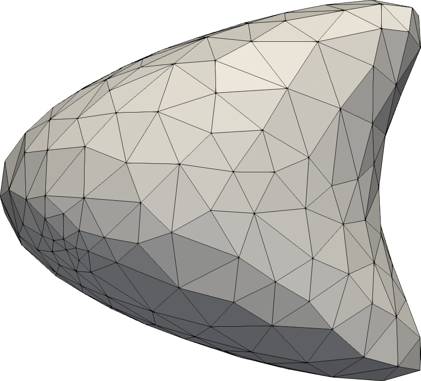
In this example, we consider the model problem (2.8) on a general surface firstly introduced by Dziuk in [25]. Figure 1 show the discretized surface and its initial mesh. The exact solution solution $u(x)=x_{1}x_{2}$ and the right hand side function $f$ can be computed from $u$.

Fig. 1: Initial mesh for Dzuik surface

We report the numerical results in Table 1. As predict by the Theorem 14 and Theorem 10, the $L_{2}$ error converges at a rate of $\mathcal{O}(h^{2})$ and the discrete $H^{1}$ semi-error converges at a rate of $\mathcal{O}(h)$. Concerning the error between the finite element gradient and the gradient of the interpolation of the exact solution, $\mathcal{O}(h)$ convergence can be observed. It means that there is no supercloseness between the finite element gradient and the gradient of the interpolation of the exact solution, which is similar to the numerical results in planar domain [30]. Even though in that case, we can observe $\mathcal{O}(h^{1.9})$ superconvergence for the recovered gradient.

Table 1: Numerical results for numerical example 1

Dof	$e$	order	$De$	order	$D_{i}e$	Order	$D_{r}e$	Order
243	3.70e-02	–	6.95e-01	–	2.10e-01	0.00	3.20e-01	–
966	8.51e-03	1.07	3.66e-01	0.46	1.08e-01	0.48	1.07e-01	0.79
3858	2.19e-03	0.98	1.86e-01	0.49	5.49e-02	0.49	3.06e-02	0.90
15426	5.53e-04	0.99	9.37e-02	0.50	2.77e-02	0.50	8.28e-03	0.94
61698	1.39e-04	1.00	4.69e-02	0.50	1.39e-02	0.50	2.23e-03	0.95
246786	3.47e-05	1.00	2.35e-02	0.50	6.93e-03	0.50	6.15e-04	0.93

6.2 Numerical example 2

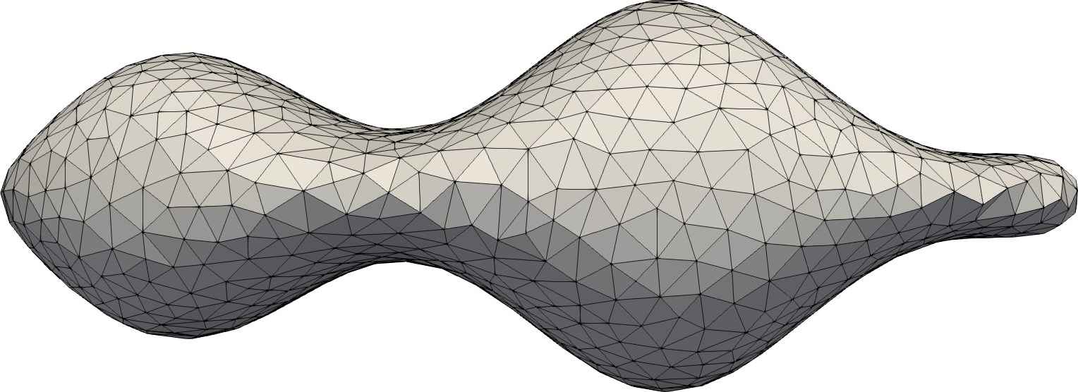
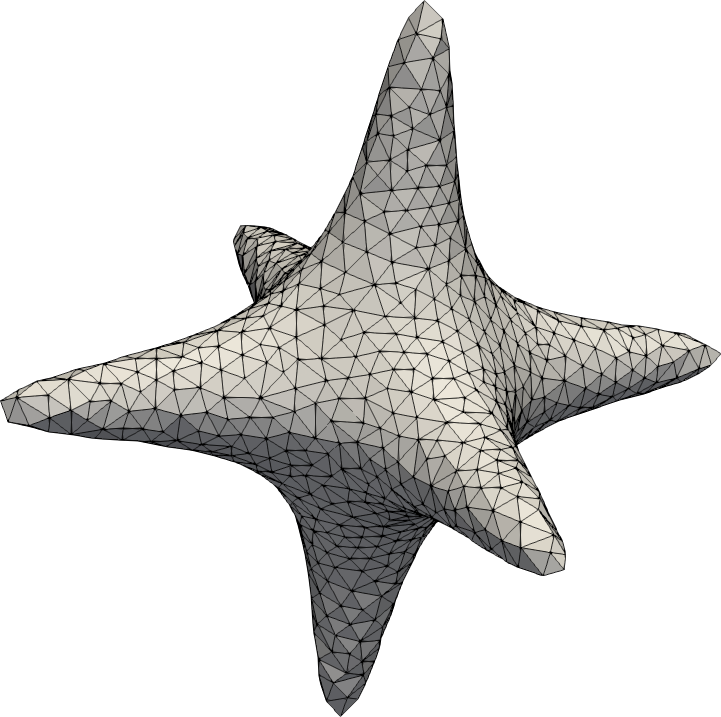
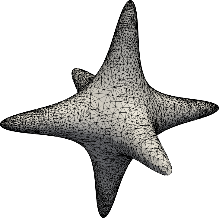
Our second example to consider a general surface with high curvature part as in [24, 26]. The discretized surface with the initial mesh was plotted in Figure 2. We choose $f$ to fit the exact solution $u(x)=x_{1}x_{2}$.

Fig. 2: Initial mesh for Elliot surface

In Table 2, we list the history of numerical errors. We can observe the same optimal convergence results in $L^{2}$ norm and discrete $H^{1}$ semi-norm which matches well with the established theoretic results in Section 4. Similar to the previous example, $\mathcal{O}(h^{2})$ can be observed even though there is no supercloseness result.

Table 2: Numerical results for numerical example 2

Dof	$e$	order	$De$	order	$D_{i}e$	Order	$D_{r}e$	Order
1153	8.82e+00	–	2.92e+01	–	2.50e+01	–	1.46e+01	–
4606	5.25e-02	3.70	4.24e-01	3.06	2.26e-01	3.40	2.37e-01	2.98
18418	3.92e-03	1.87	1.86e-01	0.60	5.37e-02	1.04	7.19e-02	0.86
73666	1.08e-03	0.93	9.28e-02	0.50	2.65e-02	0.51	1.98e-02	0.93
294658	2.54e-04	1.05	4.64e-02	0.50	1.32e-02	0.50	5.11e-03	0.98
1178626	6.23e-05	1.01	2.32e-02	0.50	6.59e-03	0.50	1.31e-03	0.98

6.3 Numerical example 3

In all the previous numerical examples, the exact solutions are smooth. In this example, we consider a benchmark problem on the unit sphere surface with a singular solution. The solution and the source term in spherical coordinates are given by

$$u=\sin^{\lambda}(\theta)\sin(\phi),\quad f=(2+\lambda^{2}+\lambda)\sin^{\lambda}(\theta)\sin(\phi)+(1-\lambda^{2})\sin^{\lambda-2}(\theta)\sin(\phi).$$

It is easy to show that $u\in H^{1+\lambda}(\Gamma)$. When $\lambda<1$, the solution $u$ has two singularities at north and south poles.

a

b

Fig. 3: Meshes for numerical example 3: (a) Initial mesh; (b) Adaptively refined mesh.

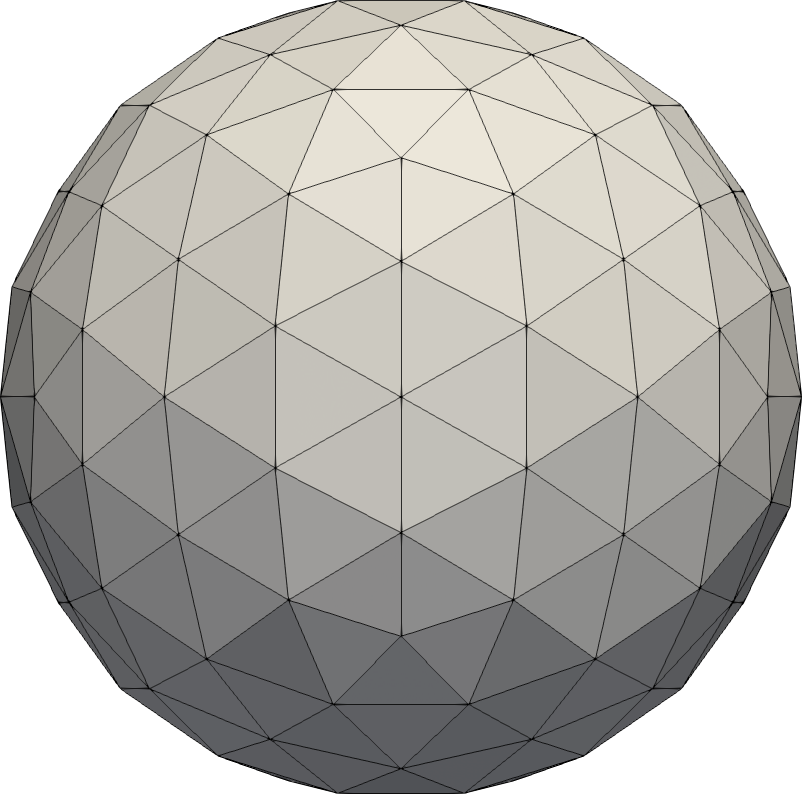
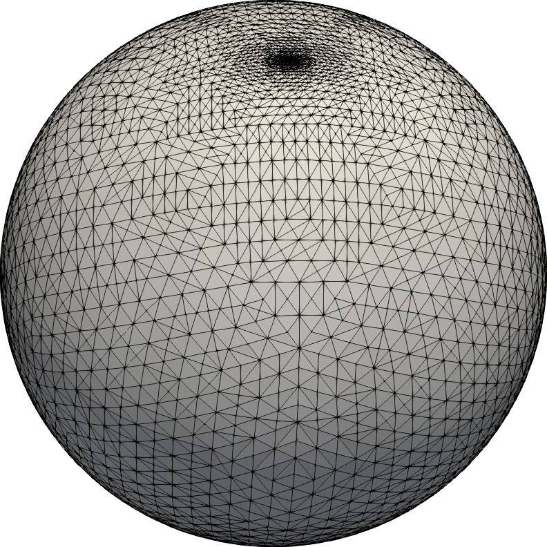
To resolve the singularity, we apply the adaptive finite element method with the recovery based a posteriori error estimator (5.82). The initial mesh is icosphere mesh as plotted in Figure 3. Figure 3 plot the adaptive refined meshes after 14 adaptive refinements. It obvious that the refinement is mainly concentrated on the two singular points. We plot the errors in Figure 4. The $L^{2}$ error and discrete $H^{1}$ semi-error both converges optimally. The recovered gradient superconverges to the exact gradient at a rate of $\mathcal{O}(h^{1.6})$.

a

b

Fig. 4: Meshes for numerical example3: (a) Initial mesh; (b) Adaptively refined mesh.

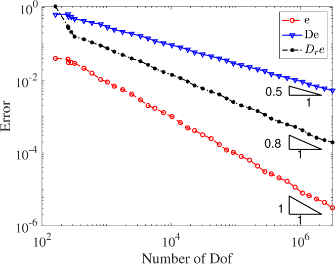
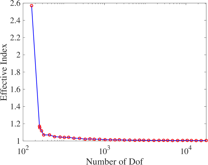
To quantify the performance of our new recovery-based a posterior error estimator for the Laplace-Beltrami problem, the effectivity index $\kappa$ is used to measure the quality of an error estimator [1, 5], which is defined by the ratio between the estimated error and the exact error

$$\kappa=\frac{\|u_{h}-\nabla u_{h}\|_{L^{2}(\Gamma}}{|u-u_{h}|_{H^{1}(\Gamma_{h};\mathcal{T}_{h})}}$$ (6.84)

The effectivity index is plotted in Figure 4 . We see that $\kappa$ converges asymptotically to $1$ which indicates the posteriori error estimator (5.82) is asymptotically exact.

a

b

Fig. 5: Meshes for numerical example 4: (a) Initial mesh; (b) Adaptively refined mesh.

6.4 Numerical example 4

This example is taken from [19]. The surface is the zero level of the following level set function

$$\phi(x)=400(x_{1}^{2}x_{2}^{2}+x_{2}^{2}x_{3}^{2}+x_{1}^{2}x_{3}^{2})-(1-x_{1}^{2}-x_{2}^{2}-x_{3}^{2})^{3}-40.$$

The discretized surface on the initial mesh is shown in Figure 5. What can be clearly seen in this figure is the high curvature parts. The initial mesh fails to resolve them. In contrast, the high curvature parts are well captured by the adaptively refined mesh as plotted in Figure 5.

a

b

Fig. 6: Meshes for numerical example 4: (a) Initial mesh; (b) Adaptively refined mesh.

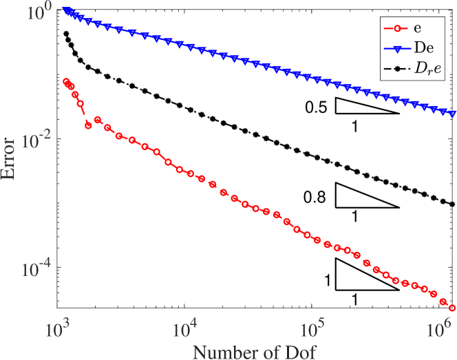
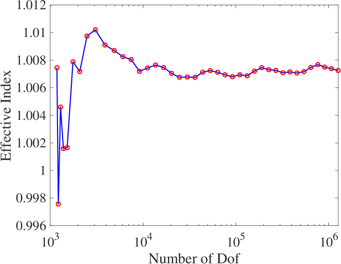
Figure 6 plot errors in term of degrees of freedom. The figure shows the optimal decay of the $L^{2}$ error and discrete $H^{1}$ semi-error. In addition, we observe that the recovered gradient error superconverges at a rate of $\mathcal{O}(h^{1.6})$. In Figure 6, we graph the effectivity index $\kappa$. Figure 2 reveals that the effectivity index is close to $1$ after several refinements. It illustrates that the recovery-type a posteriori error estimator (5.82) is asymptotically exact.

7 Conclusion

In this paper, we have introduced and analyzed the Crouzeix-Raviart element on a surface setting. The surface Crouzeix-Raviart element is a nonconforming element in the sense that it is only continuous at edge centers. The optimal convergence theory has also been established using a delicate argument. In addition, we have proposed a superconvergent gradient recovery for the surface Crouzeix-Raviart element. The proposed post-processing procedure is numerical proven to be able to provide a more accurate approximate gradient and asymptotically exact a posteriori error estimator.

Ongoing research topics include using a residue-type a posterior error estimate to conduct medius error analysis [9] and applying it to investigate surface Stokes problems and surface Naiver-Stokes problems.

References

- [1] M. Ainsworth and J. T. Oden, A posteriori error estimation in finite element analysis, Pure and Applied Mathematics (New York), Wiley-Interscience [John Wiley & Sons], New York, 2000.
- [2] P. F. Antonietti, A. Dedner, P. Madhavan, S. Stangalino, B. Stinner, and M. Verani, High order discontinuous Galerkin methods for elliptic problems on surfaces, SIAM J. Numer. Anal., 53 (2015), pp. 1145–1171.
- [3] M. Arroyo and A. DeSimone, Relaxation dynamics of fluid membranes, Phys. Rev. E, 79 (2009), p. 031915.
- [4] T. Aubin, Best constants in the Sobolev imbedding theorem: the Yamabe problem, in Seminar on Differential Geometry, vol. 102 of Ann. of Math. Stud., Princeton Univ. Press, Princeton, N.J., 1982, pp. 173–184.
- [5] I. Babuška and T. Strouboulis, The finite element method and its reliability, Numerical Mathematics and Scientific Computation, The Clarendon Press, Oxford University Press, New York, 2001.
- [6] J. W. Barrett, H. Garcke, and R. Nürnberg, Numerical computations of the dynamics of fluidic membranes and vesicles, Phys. Rev. E, 92 (2015), p. 052704.
- [7] J. W. Barrett, H. Garcke, and R. Nürnberg, A stable numerical method for the dynamics of fluidic membranes, Numerische Mathematik, 134 (2016), pp. 783–822.
- [8] D. Braess, Finite elements, Cambridge University Press, Cambridge, third ed., 2007. Theory, fast solvers, and applications in elasticity theory, Translated from the German by Larry L. Schumaker.
- [9] S. C. Brenner, Forty years of the Crouzeix-Raviart element, Numer. Methods Partial Differential Equations, 31 (2015), pp. 367–396.
- [10] S. C. Brenner and L. R. Scott, The mathematical theory of finite element methods, vol. 15 of Texts in Applied Mathematics, Springer, New York, third ed., 2008.
- [11] S. C. Brenner and L.-Y. Sung, Linear finite element methods for planar linear elasticity, Math. Comp., 59 (1992), pp. 321–338.
- [12] F. Brezzi and M. Fortin, Mixed and hybrid finite element methods, vol. 15 of Springer Series in Computational Mathematics, Springer-Verlag, New York, 1991.
- [13] E. Burman, P. Hansbo, M. G. Larson, K. Larsson, and A. Massing, Finite element approximation of the laplace–beltrami operator on a surface with boundary, Numerische Mathematik, (2018).
- [14] C. Carstensen and S. Bartels, Each averaging technique yields reliable a posteriori error control in FEM on unstructured grids. I. Low order conforming, nonconforming, and mixed FEM, Math. Comp., 71 (2002), pp. 945–969.
- [15] L. Chen, Short implementation of bisection in MATLAB, in Recent advances in computational sciences, World Sci. Publ., Hackensack, NJ, 2008, pp. 318–332.
- [16] P. G. Ciarlet, The finite element method for elliptic problems, vol. 40 of Classics in Applied Mathematics, Society for Industrial and Applied Mathematics (SIAM), Philadelphia, PA, 2002. Reprint of the 1978 original [North-Holland, Amsterdam; MR0520174 (58 #25001)].
- [17] B. Cockburn and A. Demlow, Hybridizable discontinuous Galerkin and mixed finite element methods for elliptic problems on surfaces, Math. Comp., 85 (2016), pp. 2609–2638.
- [18] M. Crouzeix and P.-A. Raviart, Conforming and nonconforming finite element methods for solving the stationary Stokes equations. I, Rev. Française Automat. Informat. Recherche Opérationnelle Sér. Rouge, 7 (1973), pp. 33–75.
- [19] A. Dedner and P. Madhavan, Adaptive discontinuous Galerkin methods on surfaces, Numer. Math., 132 (2016), pp. 369–398.
- [20] A. Dedner, P. Madhavan, and B. Stinner, Analysis of the discontinuous Galerkin method for elliptic problems on surfaces, IMA J. Numer. Anal., 33 (2013), pp. 952–973.
- [21] A. Demlow, Higher-order finite element methods and pointwise error estimates for elliptic problems on surfaces, SIAM J. Numer. Anal., 47 (2009), pp. 805–827.
- [22] A. Demlow and G. Dziuk, An adaptive finite element method for the Laplace-Beltrami operator on implicitly defined surfaces, SIAM J. Numer. Anal., 45 (2007), pp. 421–442 (electronic).
- [23] M. P. do Carmo, Riemannian geometry, Mathematics: Theory & Applications, Birkhäuser Boston, Inc., Boston, MA, 1992. Translated from the second Portuguese edition by Francis Flaherty.
- [24] G. Dong and H. Guo, Parametric polynomial preserving recovery on manifolds, arXiv:1703.06509 [math.NA], 2017.
- [25] G. Dziuk, Finite elements for the Beltrami operator on arbitrary surfaces, in Partial differential equations and calculus of variations, vol. 1357 of Lecture Notes in Math., Springer, Berlin, 1988, pp. 142–155.
- [26] G. Dziuk and C. M. Elliott, Finite element methods for surface PDEs, Acta Numer., 22 (2013), pp. 289–396.
- [27] S. Elcott, Y. Tong, E. Kanso, P. Schröder, and M. Desbrun, Stable, circulation-preserving, simplicial fluids, ACM Trans. Graph., 26 (2007).
- [28] T.-P. Fries, Higher-order surface fem for incompressible navier-stokes flows on manifolds, International Journal for Numerical Methods in Fluids, 88 (2018), pp. 55–78.
- [29] J. Grande and A. Reusken, A higher order finite element method for partial differential equations on surfaces, SIAM J. Numer. Anal., 54 (2016), pp. 388–414.
- [30] H. Guo and Z. Zhang, Gradient recovery for the Crouzeix-Raviart element, J. Sci. Comput., 64 (2015), pp. 456–476.
- [31] K. Larsson and M. G. Larson, A continuous/discontinuous Galerkin method and a priori error estimates for the biharmonic problem on surfaces, Math. Comp., 86 (2017), pp. 2613–2649.
- [32] J. M. Lee, Riemannian manifolds, vol. 176 of Graduate Texts in Mathematics, Springer-Verlag, New York, 1997. An introduction to curvature.
- [33] P. Mullen, K. Crane, D. Pavlov, Y. Tong, and M. Desbrun, Energy-preserving integrators for fluid animation, ACM Trans. Graph., 28 (2009), pp. 38:1–38:8.
- [34] M. A. Olshanskii, A. Quaini, Reusken A., and V. Yushutin, A finite element method for the surface stokes problem, arXiv:1801.06589 [math.NA], 2018.
- [35] M. A. Olshanskii, A. Reusken, and J. Grande, A finite element method for elliptic equations on surfaces, SIAM J. Numer. Anal., 47 (2009), pp. 3339–3358.
- [36] M. A. Olshanskii and D. Safin, A narrow-band unfitted finite element method for elliptic PDEs posed on surfaces, Math. Comp., 85 (2016), pp. 1549–1570.
- [37] K. Padberg-Gehle, S. Reuther, S. Praetorius, and A. Voigt, Transfer operator-based extraction of coherent features on surfaces, in Topological Methods in Data Analysis and Visualization IV, H. Carr, C. Garth, and T. Weinkauf, eds., Cham, 2017, Springer International Publishing, pp. 283–297.
- [38] A. Reusken, Stream function formulation of surface stokes equations, IMA Journal of Numerical Analysis, (2018), p. dry062.
- [39] S. Reuther and A. Voigt, Solving the incompressible surface navier-stokes equation by surface finite elements, Physics of Fluids, 30 (2018), p. 012107.
- [40] L. Rineau and M. Yvinec, 3D surface mesh generation, in CGAL User and Reference Manual, CGAL Editorial Board, 4.9 ed., 2016.
- [41] E. Sasaki, S. Takehiro, and M. Yamada, Bifurcation structure of two-dimensional viscous zonal flows on a rotating sphere, Journal of Fluid Mechanics, 774 (2015), p. 224–244.
- [42] H. Wei, L. Chen, and Y. Huang, Superconvergence and gradient recovery of linear finite elements for the Laplace-Beltrami operator on general surfaces, SIAM J. Numer. Anal., 48 (2010), pp. 1920–1943.
- [43] J. Wloka, Partial differential equations, Cambridge University Press, Cambridge, 1987. Translated from the German by C. B. Thomas and M. J. Thomas.
- [44] Z. Zhang and A. Naga, A new finite element gradient recovery method: superconvergence property, SIAM J. Sci. Comput., 26 (2005), pp. 1192–1213 (electronic).