Are smooth pseudopotentials a good choice for representing short-range interactions?

Abstract

When seeking a numerical representation of a quantum-mechanical multiparticle problem it is tempting to replace a singular short-range interaction by a smooth finite-range pseudopotential. Finite basis set expansions, e.g., in Fock space, are then guaranteed to converge exponentially. The need to faithfully represent the artificial length scale of the pseudopotential, however, places a costly burden on the basis set. Here we discuss scaling relations for the required size of the basis set and demonstrate the basis set convergence on the example of a two-dimensional system of few fermions with short-range $s$-wave interactions in a harmonic trapping potential. In particular we show that the number of harmonic-oscillator basis functions needed to reach a regime of exponential convergence for a Gaussian pseudopotential scales with the fourth power of the pseudopotential length scale, which can be improved to quadratic scaling when the basis functions are rescaled appropriately. Numerical examples for three fermions with up to a few hundred single-particle basis functions are presented and implications for the feasibility of accurate numerical multiparticle simulations of interacting ultracold-atom systems are discussed.

I Introduction

There is increasing interest in the theoretical description of multiparticle systems of interacting ultracold atoms thanks to the recent progress in experimental realizations Cheuk et al. (2016); Feld et al. (2011); Zürn et al. (2013); Mazurenko et al. (2017); Hueck et al. (2018). In particular we may expect exciting developments in microtraps Serwane et al. (2011); Zürn et al. (2012); Kaufman et al. (2014) with tens of particles where accessing strongly correlated regimes of quantum-Hall-like physics seems feasible Popp et al. (2004); Viefers (2008); Regnault and Jolicoeur (2004); Möller et al. (2009).

The theoretical description of atom-atom interactions is significantly simplified at ultracold temperatures where details of the interaction potentials can be neglected in favor of a single constant, the $s$-wave scattering length $a_{s}$, to define a physical model with contact interactions Pethick and Smith (2002). Despite these simplifications, the complexity of many-particle quantum mechanics still makes it a very difficult problem to solve, where exact solutions are only available in special cases in one spatial dimension Lieb and Liniger (1963); Yang (1967); Gaudin (1967); Volosniev et al. (2014); Deuretzbacher et al. (2008) or for up to three particles in a harmonic trap Busch et al. (1998); Liu et al. (2010a, b).

A straightforward and generalist approach to representing the many-body problem for computational treatment is to introduce a discrete and necessarily finite basis of smooth single-particle wave functions from which a finite but still potentially very large Fock-space is constructed to represent the many-body Hamiltonian as a matrix. Finding eigenstates and eigenvalues of the full matrix is known as exact diagonalization or full configuration-interaction Deuretzbacher et al. (2007); Rontani et al. (2009); García-March et al. (2013); Dehkharghani et al. (2015); Mujal et al. (2017), but many different approximation schemes have also been followed Marcin Płodzień et al. (2018). In particular, standard approaches of ab initio quantum chemistry or nuclear physics like the coupled-cluster Grining et al. (2015) or multi configurational self-consistent field theory Meyer et al. (2009) all can be formulated in this language as they rely on an underlying single-particle basis. Also Monte Carlo (or other) approaches that rely on a lattice discretization of continuous space fall into the same category Carlson et al. (2011), as the underlying single-particle space can be represented as a discrete set of plane waves.

One of the complications in the numerical treatment of contact interactions with basis set expansions stems from the nonanalytic behavior of the wave function at the point of particle coalescence. At this point, the appropriate Bethe-Peierls boundary conditions demand a cusp in one spatial dimension, i.e. a point of nondifferentiability Lieb and Liniger (1963), in two dimensions a logarithmic divergence, and in three dimension a $1/r$ divergence of the wave function Bethe and Peierls (1935); Olshanii and Dunjko (2003); Werner and Castin (2012). While in one dimension a Dirac $\delta$ function pseudopotential provides a well-defined model for contact interactions, the convergence of basis set expansions is algebraic and painfully slow Grining et al. (2015); Jeszenszki et al. (2018a). Basis set expansions in two and three dimensions diverge for bare contact interaction Esry and Greene (1999); Doganov et al. (2013); Rontani et al. (2017) and basis-set-dependent renormalization procedures have to be used in order to obtain convergent and correct results Castin (2004); Ernst et al. (2011); Rontani et al. (2017); Luo et al. (2016). In the best case, renormalized contact interactions will lead to algebraic convergence in the size of the finite single-particle basis set Carlson et al. (2011); Werner and Castin (2012); Jeszenszki et al. (2018a). Some of us have recently described a transcorrelated method where the singular nature of the contact interaction is reduced by means of a similarity transformation of the Hamiltonian Jeszenszki et al. (2018a) (see also Ref. Rotureau (2013) for a related idea). This promising approach results in an improved power-law scaling but the convergence still remains algebraic.

Here, we consider a different approach where the contact interaction is replaced by a smooth finite-range pseudopotential. This has the advantage that basis set expansions will converge exponentially for appropriately chosen single-particle basis functions Mercier (2014). Specifically we consider what the requirements are for the basis set to reach the regime of exponential convergence and whether this approach is feasible for multiparticle simulations. Examples of finite-range pseudopotentials used in the literature are the Troullier-Martins Bugnion et al. (2014); Whitehead et al. (2016), Pöschl-Teller Forbes et al. (2011); Galea et al. (2016), and Gaussian potentials Christensson et al. (2009); von Stecher et al. (2008, 2007); Yan and Blume (2014); Yin et al. (2014); Doganov et al. (2013); Imran and Ahsan (2015); Klaiman et al. (2014); Beinke et al. (2015); Bolsinger et al. (2017a, b); Mujal et al. (2017, 2018), in addition to the square well popular in diffusion Monte Carlo simulationsvon Stecher et al. (2008).

When using finite range pseudopotentials to represent short-range interactions, an interpolation in the width of the pseudopotential should be done to the zero-range limit Blume (2012). In order to approach this limit, the length scale of the pseudopotential should be significantly smaller than other physically relevant length scales of the problem, in particular the mean particle separation and length scales imposed by external potentials. In order to reach a regime where the basis set expansion converges exponentially, however, the basis set needs to resolve the smallest length scale of the pseudopotential. At the same time, the large length scales of the problem, i.e., the (Thomas-Fermi) size of the cold atom cloud, or the size of the container, also have to be represented by the basis set. This hierarchy of length scales, typically spanning at least one but possibly several orders of magnitude, presents a challenge for accurate numerical simulations. While the size of the single-particle basis (quantified by the number of single-particle functions $M$) is determined by this hierarchy of length scales, the size of the full many-body problem also depends strongly on the number of particles $N$. Specifically for spinless bosons, the size of the relevant part of Fock space is $\binom{N+M-1}{M}$, whereas for spin-$\frac{1}{2}$ fermions the total dimension is $\binom{M}{N_{\uparrow}}\binom{M}{N_{\downarrow}}$, where $N_{\uparrow}$ and $N_{\downarrow}$ are the numbers of up- and down-spin particles, respectively.

In this work, we specifically consider ultracold fermionic atoms in a harmonic oscillator trapping potential where the potential in one of the three trapping directions is so tight that the problem can be considered two-dimensional. We furthermore choose a Gaussian pseudopotential to model attractive $s$-wave interactions between spin-up and spin-down particles Jeszenszki et al. (2018b). For the underlying single-particle basis we consider two cases: (1) a basis that is defined by the single-particle eigenstates of the isotropic two-dimensional harmonic trapping potential, and (2) the same set of basis functions with scaled spatial coordinates by a scaling factor $\gamma$. Using the known properties of the harmonic oscillator eigenfunctions we show that the basis set size $M$ required to resolve the chosen length scale of the pseudopotential $l_{\mathrm{res}}$ scales as $(l/l_{\mathrm{res}})^{4}$ where $l=\sqrt{\hbar/m\omega}$ is the harmonic oscillator length scale of the trapping potential for case (1).

Allowing the basis functions to be scaled by $\gamma$ as in case (2) leads to an improved scaling of $(l/l_{\mathrm{res}})^{2}$ while still faithfully resolving the small length scale $l_{\mathrm{res}}$ and a fixed large length scale that is determined by the particle-number and interaction strength. We provide estimates for these length scales and the required scaling parameters. Numerical examples show the convergence of the ground-state energy for three fermions obtained by exact diagonalization with single-particle basis sets of up to 231 Fock-Darwin orbitals. In order to compute the matrix elements of the Gaussian interaction potential with the Fock-Darwin basis of this size, a careful algorithm based on recursion formulas had to be developed in order to avoid an excessive accumulation of round-off errors. This algorithm is described in Appendix B.

This paper is organized as follows: After defining the Hamiltonian in Sec. II and introducing the methodology in Sec. III, we discuss the main results of the paper in Sec. IV. Examples for the numerical convergence with a harmonic oscillator basis are presented in Sec. IV.1 before deriving analytical formulas for the required minimum basis set size in Sec. IV.2 for the unscaled and in Sec. IV.3 for a scaled harmonic oscillator basis. The required scaling factor is estimated in Sec. IV.4 where also numerical results for the scaled basis are presented. Implications of our findings for the feasibility of accurate computations of larger multiparticle problems are discussed in Sec. V. Two appendixes define the Fock-Darwin orbital basis used (Appendix A) and detail the explicit formulas and the algorithm used to compute the matrix elements (Appendix B).

II Hamiltonian

We consider ultracold fermions in a two-dimensional harmonic trap,

$$H = H_{\mathrm{osc}}+\sum_{i}^{N_{\uparrow}}\sum_{j}^{N_{\downarrow}}V({\bf r}_{i\uparrow},{\bf r}_{j\downarrow})\ ,$$ (1)

$$H_{\mathrm{osc}} = \sum_{\sigma}\sum_{i}^{N_{\sigma}}\left(-\frac{\hbar^{2}}{2m}\nabla^{2}_{i\sigma}\ +\ \frac{m\omega^{2}}{2}r_{i\sigma}^{2}\right)\ ,$$ (2)

where $m$ is the mass of the fermions, $\omega$ is the harmonic oscillator strength, $r_{i\sigma}$ is the position of the $i$th particle with the spin $\sigma$, and $V({\bf r}_{i\uparrow},{\bf r}_{j\downarrow})$ is the interaction potential between the fermions. Dividing the operator $H_{\mathrm{osc}}$ with $\hbar\omega$, Eq. (2) takes the form

$$\frac{H_{\mathrm{osc}}}{\hbar\omega} = \sum_{\sigma}\sum_{i}^{N_{\sigma}}\left(-\frac{l^{2}}{2}\nabla^{2}_{i\sigma}\ +\ \frac{1}{2l^{2}}r_{i\sigma}^{2}\right)\ ,$$

where $l=\sqrt{\frac{\hbar}{m\omega}}$ is the harmonic oscillator length scale of the trapping potential. The interaction between the particles is described with a Gaussian pseudopotential

$$V({\bf r}_{i\uparrow},{\bf r}_{j\downarrow}) = -\frac{V_{0}}{R^{2}}\,e^{-\frac{\left({\bf r}_{i\uparrow}-{\bf r}_{j\downarrow}\right)^{2}}{R^{2}}}\ .$$ (3)

The parameters $V_{0}$ and $R$ control the strength and width of the interaction potential, respectively. These parameters can be converted to the $s$-wave scattering length using a simple approximate formula Jeszenszki et al. (2018b),

$$\frac{a_{s}}{R} = \sqrt{2}\,\exp\left(-\frac{3\gamma_{E}}{2}+\frac{8\hbar^{2}}{V_{0}m}+\sum_{i}^{n}\alpha_{i}\frac{V_{0}}{V_{0}-W_{i}}\right)\ ,$$ (4)

where $a_{s}$ is the $s$-wave scattering length in two dimensions, $\gamma_{E}$ is the Euler-Mascheroni constant with the approximate value of $\gamma_{\mathrm{E}}\approx 0.577216$, and $\alpha_{i}$ and $W_{i}$ are parameters fitted to direct numerical calculations . Accurate numerical values of the parameters are given in Table III. in Ref. Jeszenszki et al. (2018b) for $i\leq 4$. Alternatively, more complicated numerical approaches can be applied Verhaar et al. (1985); Jeszenszki et al. (2018b).

III Basis-set expansion

For our numerical approach, we compute the ground-state energy of a multiple-fermion system following the exact diagonalization approach. Starting from a finite single-particle basis of size $M$ (i.e., with $M$ spin orbitals), the multiparticle wave function is expanded as a linear combination

$$|\Psi\rangle=\sum_{\underline{n}}C_{\underline{n}}|\Phi_{\underline{n}}\rangle,$$ (5)

of states in the Fock basis

$$|\Phi_{\underline{n}}\rangle=\displaystyle\prod_{i=1}^{M}(\hat{c}_{i}^{\dagger})^{n_{i}}|\mathrm{vac}\rangle,$$ (6)

where $\underline{n}=(n_{1},\ldots,n_{i},\ldots,n_{M})$ and $n_{i}$ is the occupation number of the $n$th single-particle basis function (spinr orbital). The fermionic Fock states $|\Phi_{\underline{n}}\rangle$ (often referred to as Slater determinants) are constructed from the complete set of index vectors $\underline{n}$ for fixed particle number $N$, with

$$N=\sum_{i=1}^{M}n_{i}.$$ (7)

The exact diagonalization approach (also referred to as full configuration interaction) refers to considering the multiparticle Hamiltonian (1) with the chosen particle-number content projected onto the basis of states (6) as a matrix and finding its eigenvalues and eigenvectors.

In this paper we use a single-particle basis constructed from the spinful eigenstates of the two-dimensional harmonic oscillator (2). The explicit form of the basis functions used in the numerical procedure is presented in Appendix A. Even though the one-body and two-body integrals needed for the relevant matrix elements can be expressed analytically (see, e.g., Ref. Mujal et al. (2017)), obtaining accurate numerical values is challenging due to the proliferation of rounding errors during floating-point arithmetic. We have therefore developed an iterative algorithm for the evaluation of the two-body integrals, which alleviates this problem. The details are presented in Appendix B.

For the numerical procedure we determine the ground-state energy

$$E=\min_{C_{\underline{n}}}\frac{\langle\Psi|H|\Psi\rangle}{\langle\Psi|\Psi\rangle}\equiv\langle H\rangle,$$ (8)

with a matrix-free approach: Using a variant of the power method Mises and Pollaczek-Geiringer (1929), we iteratively rotate an initial state onto the ground state vector without having to construct the matrix explicitly. Numerical computations are done using the NECI nec software in deterministic mode. Even larger Hilbert spaces could be explored using stochastic algorithms for exact diagonalization such as Full Configuration Interaction Quantum Monte Carlo (FCIQMC) Booth et al. (2009).

IV Resolving the Gaussian pseudopotential

IV.1 Unscaled harmonic oscillator basis

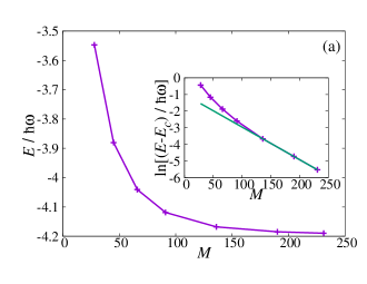
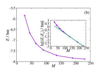
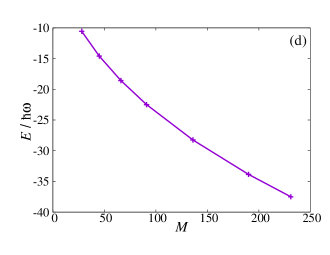
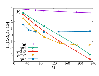
Figure 1 shows the ground state energy of three interacting fermions (two spin-up and one spin-down) according to the Hamiltonian (1) after full diagonalization with a finite Fock basis. We are using the Fock-Darwin form (A) of the (unscaled) harmonic oscillator eigenfunctions of the single-particle Hamiltonian (2) up to shell $n=20$, which yields up to $M=231$ single-particle basis functions. The maximal dimension of the computational Hilbert space for the three fermions with the zero total angular momentum slot is $\approx 1.6\times 10^{5}$, which is already a significant size for the deterministic diagonalization with available computational resources.

It is clearly seen in Fig. 1 that these basis set sizes are not sufficient to enter a regime of exponential convergence except for Figs. 1(a) and 1(b), where this regime is reached for the last few data points as seen from the insets. In these cases the width of the pseudopotential $R\approx l$ is close to the length scale of the trapping potential. Since the mean particle separation in the harmonic trap will also be of the same order $l$, or even smaller, this pseudopotential does not provide a useful approximation for the zero-range contact interactions that are relevant for modeling experiments with ultracold neutral atoms. As the lowest energy values reached for each pseudopotential width $R$ change significantly between the different panels of Fig. 1, it is also apparent that $R\ll l$ is a necessary condition for a useful, convergent approximation of the zero-range limit. Even without more sophisticated analysis, it is apparent from the results of Fig. 1 that the necessary extrapolations the infinite basis set ($M\to\infty$) and zero-range ($R\to 0$) limit will be challenging to achieve.

Figure 1: Convergence of the ground-state energy for three fermions with attractive Gaussian pseudopotential interactions in the unscaled harmonic oscillator basis. The energy from exact diagonalization in the finite multiparticle basis of Eq. (6) is plotted vs the size $M$ of the single-particle basis for Gaussian pseudopotentials of different widths $R$: (a) $R=l$, (b) $R=0.8l$, (c) $R=0.3l$, and (d) $R=0.1l$, where $l=\sqrt{\hbar/m\omega}$ is the length scale of the harmonic trapping potential. The insets in Figs. 1(a) and 1(b) show logarithmic plots of the same data as the main graph and demonstrate that a regime of exponential convergence is reached. The extrapolated limiting values of the energy $E_{c}$ are obtained by nonlinear fitting of the exponential function $Ae^{-BM}+E_{c}$ to the last three data points: (a) $E_{c}=-4.19359\hbar\omega$ and (b) $E_{c}=-7.93323\hbar\omega$. The interaction strength $\ln(l/a_{s})=3.0$ is kept constant for all panels and the corresponding amplitude parameters $V_{0}$ are determined numerically following the procedure described in Ref. Jeszenszki et al. (2018b): (a) $V_{0}=19.8237\hbar\omega$, (b) $V_{0}=19.6329\hbar\omega$, (c) $V_{0}=18.2369\hbar\omega$, and (d) $V_{0}=13.024\hbar\omega$.

IV.2 Length scale resolution

Since we are using a smooth Gaussian pseudopotential, we should expect that, for a sufficiently large basis set, the energy will converge exponentially to a limiting value with the size of the single-particle basis set. Indeed, it is well known that the Fourier transform of a Gaussian function yields again a Gaussian, which decays, in fact, faster than exponential in the tails. Sampling a Gaussian potential function in momentum space, should thus lead to at least exponential convergence, once the basis set is large enough to sample the tails of the Fourier-transformed Gaussian in momentum space. The necessary condition to reach this regime is that the basis set can resolve length scales that are smaller than the length scale $R$ of the Gaussian.

We now use this argument as a motivation to consider the length scale resolution of a two-dimensional harmonic oscillator basis. In order to keep the basis set independent from the Hamiltonian of Eq. (2), we consider basis functions that are eigenfunctions of a harmonic oscillator with frequency $\tilde{\omega}$ and corresponding length scale $\tilde{l}=\sqrt{\hbar/m\tilde{\omega}}$. For a one-dimensional harmonic oscillator, the $p$th excited state has a spatial extent that can be estimated by the classical turning point $x_{t}$:

$$(p+\frac{1}{2})\hbar\tilde{\omega}=\frac{1}{2}m\tilde{\omega}^{2}x_{t}^{2},$$ (9)

or $x_{t}=\sqrt{2p+1}\,\tilde{l}$. The set of $M_{\mathrm{1D}}=p+1$ harmonic oscillator functions up to the $p$th excited states provides an approximately homogeneous sampling of the interval $[-x_{t},x_{t}]$ at a length scale

$$l_{\mathrm{res}}=\frac{2x_{t}}{M_{\mathrm{1D}}}=\frac{2\sqrt{2p+1}}{p+1}\tilde{l}.$$ (10)

In order to connect this result to the number $M$ of two-dimensional harmonic oscillator basis functions, we construct the latter as a product basis (of Hermite functions) with an energy cutoff. This yields

$$M =\sum_{i,j=0}^{i+j\leq p}1=\frac{(p+1)(p+2)}{2}\ .$$ (11)

We can thus relate the resolution length scale $l_{\mathrm{res}}$ to the size of the basis and obtain

$$l_{\mathrm{res}} =\frac{4\sqrt{\sqrt{8M+1}-2}}{\sqrt{8M+1}-1}\tilde{l},$$ (12)

which can be solved for $M$ to yield

$$M\approx 32\left(\frac{\tilde{l}}{l_{\mathrm{res}}}\right)^{4},$$ (13)

where lower order terms were neglected assuming $\tilde{l}\gg l_{\mathrm{res}}$.

Equation (13) provides an estimate for the size of the single-particle basis needed to resolve a length scale $l_{\mathrm{res}}$. For the situation of Sec. IV.1 where $\tilde{l}=l$ we can estimate the minimum size of the basis set to be able to resolve the pseudopotential length scale $R$ as

$$M_{\mathrm{min}}\approx 32\left(\frac{l}{R}\right)^{4},$$ (14)

i.e. the required basis set size increases rapidly when the length scale $R$ (and thus the range) of the pseudopotential is decreased.

Specifically, it means that reaching an exponentially convergent regime should be quite achievable when the pseudopotential width is of the same order of magnitude as the oscillator length $l$. For $R=l$ and $R=0.8l$ we would require a minimum of 32 and 78 single-particle basis functions, respectively, which means about 16,000 and 200,000 Fock states for three fermions. This is consistent with the numerical results of Fig. 1 obtained with up to $M=230$ single-particle basis functions.

In order to explore the physics of short-range interactions, however, we may need to use narrower pseudopotentials. With modest choices of $R=0.3l$ and $R=0.1l$ the number of required single-particle basis functions already increases to about 4,000 and 300,000, respectively, corresponding to about $3\times 10^{10}$ and $1\times 10^{16}$ multiparticle basis functions. In this case, even the storage of the wave function is very expensive as it would require 0.2 and 100,000 terabytes of memory, respectively. Although exploiting symmetries, using approximation schemes, or stochastic sampling techniques can reduce these requirements Booth et al. (2009); Christensson et al. (2009), the quartic scaling in Eq. (13) does not seem pleasant.

IV.3 Scaled harmonic oscillator basis

The required size of the single-particle basis can be decreased by introducing an appropriate scaling of the basis functions. The main idea is the following: Increasing the number of basis functions not only improves the resolution length scale $l_{\mathrm{res}}$ (by making it smaller) but also increases the largest length scale that can be described by the basis, which is given by $2x_{t}=2\sqrt{2p+1}\;\tilde{l}$, i.e., through the classical turning point. This means that the basis functions can be scaled according to the basis set size while still resolving the largest length scale of the problem (e.g., twice the Thomas-Fermi radius of a cold atomic cloud). Let us denote this largest relevant length scale as $\gamma l$, where $\gamma$ is the dimensionless form of this length scale in units of the length scale $l$ of the trapping potential. Note that $\gamma$ is determined by the physical properties of the system (i.e., particle number, interaction strength, etc.) and is thus independent of the basis set size. For the required basis set length scale we then obtain

$$\tilde{l}=\frac{\gamma}{2\sqrt{2p+1}}l\ .$$ (15)

With Eq. (10) this yields $l_{\mathrm{res}}=\gamma l/(p+1)$ and using Eq. (11) to solve for $M$ we obtain

$$M=\frac{\gamma^{2}}{2}\left(\frac{l}{l_{\mathrm{res}}}\right)^{2}+\frac{\gamma}{2}\frac{l}{l_{\mathrm{res}}}\ .$$ (16)

Applying this result to the problem of resolving a Gaussian pseudopotential with length scale $l_{\mathrm{res}}=R$ and taking the leading term for $l\gg R$, we obtain the revised relation for the minimum size of the single-particle basis,

$$M_{\mathrm{min}}\approx\frac{\gamma^{2}}{2}\left(\frac{l}{R}\right)^{2},$$ (17)

when the length scale of the single-particle basis is optimally scaled with the size of the basis set. Compared to the result (14) for the unscaled basis, the power-law scaling of the required basis set size with the pseudopotential length scale $R$ in Eq. (17) is improved by two orders.

IV.4 Estimating the interaction-dependent prefactor

As $\gamma l$ represents the largest length scale that has to be resolved by the single-particle basis, i.e., the maximal spatial extent of the system, the factor $\gamma$ depends on the details of the Hamiltonian, which, for our example, are the particle number content and the strength of the contact interaction. Although the exact value of $\gamma$ is difficult to calculate we can estimate its value and present upper and lower bounds from limiting cases that are simple to analyze.

Specifically for fermions with attractive short-range interactions as per Eq. (1), the size of the trapped noninteracting gas cloud will provide an upper bound, while a lower bound can be obtained from the strongly interacting limit where fermion pairs form deeply bound composite bosons while excess fermions remain with little residual interactions.

Starting with the upper bound, we consider a noninteracting Fermi gas with a possibly unequal population of spin-up and spin-down fermions. The largest length scale is determined by the Fermi pressure of the majority component with the quantum number $p^{\mathrm{majority}}$ along a single spatial dimension

$$\gamma_{\mathrm{upper}} = 2\sqrt{2p^{\mathrm{majority}}+1}\ .$$ (18)

The parameter $p^{\mathrm{majority}}$ can be expressed in terms of particle number $N_{\mathrm{majority}}$ by considering Eq. (11) and using the information that only one particle can occupy one spatial orbital from the same spin component to yield

$$\gamma_{\mathrm{upper}} = 2\sqrt{2\left\lceil\frac{\sqrt{8N_{\mathrm{majority}}+1}-3}{2}\right\rceil+1}\ ,$$ (19)

where $\left\lceil x\right\rceil$ is the ceiling function Eric W. Weisstein (2018a).

For strong short-range attractive interactions, pairs of spin-up and spin-down particles form point like effective bosons Levinsen and Parish (2015); Petrov et al. (2003). The interactions between the effective bosons are repulsive but vanish in the limit of strong attraction between fermions. In this limit we thus obtain a noninteracting system where all of the bosons occupy the lowest single-particle orbital. In the spin-balanced system, the largest length scale will thus be given by the length scale of the harmonic oscillator trapping potential. This length scale provides a lower bound of the largest length scale of the system as the effective repulsive interactions can only increase the average particle-particle distance. We thus obtain a lower bound of

$$\gamma^{\mathrm{sb}}_{\mathrm{lower}} = 2\ ,$$ (20)

where the index ‘$\mathrm{sb}$’ stands for the spin balanced case.

In the spin-imbalanced case, excess fermions from the majority component that are not locked-up in effective bosons who will maintain Fermi pressure. Indeed, the excess fermions have weak repulsive interactions with the effective bosons that also vanish in the strongly interacting limit (regarding the original interactions between fermions) Levinsen and Parish (2015); Petrov et al. (2003). Hence, the lower bound for the largest length scale can be tightened by considering a noninteracting Fermi gas of the excess fermions following the same argument as above. We obtain

$$\gamma^{\mathrm{si}}_{\mathrm{lower}}=2\sqrt{2\left\lceil\frac{\sqrt{8\left|N_{\uparrow}-N_{\downarrow}\right|+1}-3}{2}\right\rceil+1}\ ,$$ (21)

where the index "$\mathrm{si}$" stands for the spin-imbalanced case.

We can see from Eqs. (19) and (21) that the largest relevant length scale $\gamma l$ increases with particle number. To leading order the bounds become

$$\gamma_{\mathrm{upper}} \approx 2\sqrt[4]{8N_{\mathrm{majority}}}\ ,$$ (22)

$$\gamma_{\mathrm{lower}}^{\mathrm{si}} \approx 2\sqrt[4]{8\left|N_{\uparrow}-N_{\downarrow}\right|}\ .$$ (23)

Comparing with expression (17) for the minimum size of the single-particle basis, we see that $M_{\mathrm{min}}$ increases with the square root of the particle number (that is $N_{\mathrm{majority}}$ and $|N_{\uparrow}-N_{\downarrow}|$, respectively), i.e., requiring a larger single-particle basis for a larger particle number. We also see that the largest interaction dependence of $M_{\mathrm{min}}$ can be expected in the spin-balanced case, whereas $M_{\mathrm{min}}$ will approximately remain independent of interactions for large spin polarization (e.g., polaron physics), where $N_{\mathrm{majority}}\approx|N_{\uparrow}-N_{\downarrow}|$.

For large particle numbers the large length scale $\gamma l$ is well approximated by Thomas-Fermi theory as $\gamma l=2R_{\mathrm{TF}}$, where $R_{\mathrm{TF}}$ is the Thomas-Fermi radius. In Thomas-Fermi theory, the single-particle density $n(r)$ is found from solving

$$\mu_{0}=V_{\mathrm{ext}}(r)+\mu[n(r)],$$ (24)

where $V_{\mathrm{ext}}(r)=\frac{1}{2}m\omega^{2}r^{2}$ is the external potential, $\mu[n(r)]$ represents the chemical potential at local equilibrium [from the equation of state $\mu(n)$ of the homogeneous gas], and the constant $\mu_{0}$ is the chemical potential of the finite system Pethick and Smith (2002); Giorgini et al. (2008); Ketterle and Zwierlein (2008). The Thomas-Fermi radius $R_{\mathrm{TF}}$ is then the value of $r$ where $n(r)$ drops to zero.

For our case of a two-dimensional BCS mean-field theory yields a Thomas-Fermi radius $R_{\mathrm{TF}}$ that is independent of particle interactions Randeria et al. (1989), i.e., the result (22). In the strongly interacting limit of the balanced Fermi gas, we may use the known asymptotic form of the equation of state for a two-dimensional gas of bosonic dimers Schick (1971); Cherny and Brand (2004)

$$\mu(n)=-\frac{2\pi\hbar^{2}}{m}\frac{n}{\ln\left(a_{dd}^{2}n\right)},$$ (25)

where the scattering length of bosonic dimers $a_{dd}$ is approximately $a_{dd}\approx 0.55(4)a_{s}$ Bertaina and Giorgini (2011); Petrov et al. (2003). The Thomas-Fermi radius can be determined from Eq. (24). After some algebraic manipulations we obtain

$$R_{\mathrm{TF}} \approx \sqrt{a_{dd}^{2}N_{d}+\frac{4\pi l^{4}}{a_{dd}^{2}}\ln\left(\frac{8\pi l^{4}e^{\gamma_{\mathrm{E}}+1}}{N_{d}a_{dd}^{4}}\right)}\ ,$$

where $N_{d}$ is the number of the bosonic dimers and $\gamma_{\mathrm{E}}$ is the Euler-Mascheroni constant. The resulting approximation for the scaling factor $\gamma$ is $\gamma=2R_{\mathrm{TF}}/l$.

Figure 2: Energy convergence in a scaled harmonic oscillator basis at $R=0.3l$ with different values of the factor $\gamma$. For reference, we also show results for the unscaled basis (green crosses) identical to Fig. 1(c). (b) A logarithmic representation of the same data as in (a). The extrapolated limiting value of the energy $E_{c}$ is obtained by nonlinear fitting of the exponential function $Ae^{-BM}+E_{c}$ to the last three data points of the $\gamma=2\sqrt{3}$ data with $E_{c}=-62.38392715\hbar\omega$. $V_{0}=18.2369\hbar\omega l^{2}$ corresponding to $\ln(l/a_{s})=3.0$.

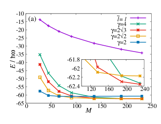
In order to test the prediction of Eq. (17) for reduced requirements for the size of a scaled single-particle basis we consider again the example of two spin-up particles and one spin-down particle with attractive interactions. The upper and lower bounds for $\gamma$ can be easily calculated from Eqs. (19) and (21) to give $\gamma_{\mathrm{upper}}=2\sqrt{3}$ and $\gamma_{\mathrm{lower}}=2$. The required minimum number of basis functions $M_{\mathrm{min}}$ from Eq. (17) then yields 20 and 60, respectively, for $R=0.3l$ [reduced from $M_{\mathrm{min}}\approx$ 4,000 for the unscaled basis according to Eq. (14)]. Similarly for $R=0.1l$ the number decreases from 300,000 to 200–600 basis functions. In Fig. 2 we show the ground-state energy $R=0.3l$ with different scaling factors $\gamma$. The results demonstrate that the regime of exponential convergence can be reached with the scaled basis, even though it was unattainable with the unscaled basis with the available computational resources. The smallest scaling factors of $\gamma=2$ and $\gamma=2\sqrt{2}$ are seen to result in an (unphysical) energy bias. This can be understood by the fact that the lower bound $\gamma=2$ and $\gamma=2\sqrt{2}$ underestimate the system size and thus the scaled basis set does not cover the whole area occupied by finite particle density. Increasing the value of $\gamma$ from the lower bound eliminates the bias but also eventually leads to a reduced convergence rate. At the upper bound ($\gamma=2\sqrt{3}$) the computation is seemingly free of bias but convergence of the energy is greatly improved compared to the unscaled basis set. Hence, we find that the upper bound can safely be used for the accurate determination of the ground-state energy.

Extrapolating our results to larger particle numbers, we need to consider the following issues: First, adding more particles at constant $M$ increases the size of Hilbert space (and thus computational complexity) due to the binomial scaling with $N$ and $M$. Whether the size $M$ of the single-particle basis has to be changed depends on how the relevant length scales change. The smallest length scale only depends on the choice of the pseudopotential and is invariant with particle number. Thus the required $M$ for the unscaled harmonic oscillator basis is independent of particle number (as long as $M$ is larger than the majority-component particle number). For the scaled-basis approach we have to consider that the relevant largest length scale may change. For example, adding another particle in the minority component (say going from three to four fermions where two are spin-up and two are spin-down) will compress the wave function towards the center of the trap for attractive interactions and thus reduce the size of the relative wave function. Also the center-of-mass wave function will shrink due to the larger total mass. Therefore, an even smaller value of $\gamma$ can be applied leading to smaller $M_{\mathrm{min}}$. However, if the number of the particles in the majority component exceeds three particles, one of the particles in the noninteracting case occupies the next shell, which increases the size of the system and the upper bound for $\gamma$ increases to $\gamma_{\mathrm{upper}}=2\sqrt{5}$. In this case, the number of single-particle basis functions increases to $M_{\mathrm{min}}\approx 120$, which is still much less than the required number of the unscaled basis functions, $M_{\mathrm{min}}\approx 4000$. The increment of $M_{\mathrm{min}}$ is less severe for larger particle numbers, again due to the effect of attractive interactions. Using $M_{\mathrm{min}}\approx 250$ scaled single-particle basis functions, we can describe about 15 particles in the majority component, which can be 30 particles in the spin-balanced case. For repulsive interaction, the relevant largest length scale of the system, the Thomas-Fermi radius, will generally increase with interaction strength leading to a larger scaling factor $\gamma$.

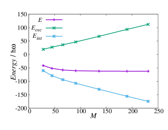
Finally, we would like to illustrate that accessing the regime of exponential convergence is significantly easier for the total energy than for other physical quantities that more sensitively probe the short-range correlations in the wave function. Let us examine the energy partition $E=E_{\mathrm{osc}}+E_{\mathrm{int}}$, where $E_{\mathrm{osc}}=\langle H_{\mathrm{osc}}\rangle$ collects the single-particle contributions of kinetic and potential energy [see Eq. (1)] , and the interaction energy $E_{\mathrm{int}}$ probes the two-particle density matrix. While both quantities reach exponential convergence for $R=l$ and $R=0.8l$ in a similar way as the total energy (data not shown), they do not converge for the narrower Gaussians within the available range of $M$. Figure 3 demonstrates this behavior for $R=0.3l$ where the total energy seemingly converges and does not significantly change for $M>100$ on the scale of the plot, but the single-particle and interaction energy parts still show a strong $M$-dependence within the accessible range of basis set sizes. While $E_{\mathrm{osc}}$ and $E_{\mathrm{int}}$ serve as useful and sensitive measures of low-order correlations for finite-size Gaussian pseudopotentials, please note that they lose meaning in the zero range limit $R\to 0$ where they separately diverge. Only the sum (i.e., the total energy) remains meaningful, which is a known feature of zero-range pseudopotentials in two and three dimensions Busch et al. (1998).

Figure 3: Convergence of energy components with respect to increasing size of the single-particle basis set $M$. While the total energy $E=E_{\mathrm{osc}}+E_{\mathrm{int}}$ converges nicely with increasing $M$ at $R=0.3l$ and $\gamma=2\sqrt{3}$ (data from Fig. 2), the single-particle part of the energy $E_{\mathrm{osc}}$ and the interaction energy $E_{\mathrm{int}}$, which more sensitively probe short-range correlations in the wave function, have not yet separately converged within the accessible range of $M$ values.

V Conclusion and outlook

In this work we considered the question whether smooth pseudopotentials are a good choice for representing short-range interactions in numerical approaches that rely on a Fock-state basis constructed from a finite set of single-particle functions. The combination of smooth pseudopotentials and an asymptotically complete set of (smooth) single-particle basis functions promises exponential convergence. This regime of exponential convergence can only be reached, however, if the basis set is large enough to resolve the relevant the length scales of the problem.

In order to isolate the effects of the single-particle basis we have used an exact diagonalization procedure to capture the many-particle quantum physics. For an example system of experimental interest (a two-dimensional harmonic trapping potential with attractively-interacting fermions) we have derived simple expressions for the required minimum size of the single-particle basis in order to resolve a given pseudopotential length scale. The algebraic scaling of $l_{\mathrm{res}}^{1/4}$ can be improved to $l_{\mathrm{res}}^{1/2}$ by scaling the basis set but remains algebraic with the required resolution length scale. An additional algebraic scaling of the required basis set size is found to apply to the particle number. With numerical example calculations for three particles we could demonstrate that the exponential convergence regime could indeed be reached, albeit in a regime where the pseudopotential length scale is not much smaller than the particle separation of length scale of the trapping potential.

In order to faithfully represent the physics of short-range interacting particles, as is relevant for ultracold quantum gases of neutral atoms, it would be necessary to reduce the length scale of the pseudopotential much further and extrapolate to the zero range limit. Although such extrapolation has been demonstrated in few-body systems using different computational approaches Blume (2012), it does not seem feasible for the current approach. Looking towards the treatment of larger particle numbers and simultaneous extrapolation to the zero-range limit, one has to consider that the benefits of asymptotically exponential convergence of the single-particle basis are counteracted by the algebraically scaling requirements for the minimum size of the single-particle basis, both with particle number and with the ratio of extremal length scales that have to be resolved.

It would be interesting to examine the basis set convergence in Jacobi coordinates, where one, typically large, length scale can be removed by separating out the center-of-mass motion. The center-of-mass length scale can become the largest length scale in the system at strong attractive interaction and weak trapping (e.g., for low-mass bright solitons or droplets), and hence its elimination from the numerical calculations should accelerate the convergence properties according to the arguments discussed in Sec. IV. In addition, the overall computational complexity is reduced by eliminating the center-of-mass degrees of freedom. Calculations in Jacobi coordinates have been performed, e.g., for three particles in one dimension Harshman (2012); García-March et al. (2014). Extensions to higher dimensions and larger particle numbers are complicated by the fact that fermionic or bosonic permutation symmetries manifest themselves by more complex symmetries in Jacobi coordinates that are more difficult to treat Harshman (2012).

A remaining alternative approach is to replace the smooth pseudopotential by a renormalized contact interaction. This has the advantage of removing the artificial length scale of the pseudopotential, while at the same time the property of exponential convergence is lost and replaced by algebraic convergence Werner and Castin (2012); Jeszenszki et al. (2018a). Extrapolation to the limit of zero range interactions has been successfully demonstrated for up to 66 fermions in three dimensions with an auxiliary-field quantum Monte Carlo approach Carlson et al. (2011). Recently developed approaches like the transcorrelated method for short-range interactions can further improve the power-law scaling Jeszenszki et al. (2018a). Extending the applicability of this method to trapped systems is a promising avenue for future work.

VI Acknowledgement

We thank Tal Levy for initial work on this project, which indicated the inadequacy of conventional basis set expansions and motivated the analysis presented in this paper. This work was supported by the Marsden Fund of New Zealand (Contract No. MAU1604), from government funding managed by the Royal Society Te Apārangi.

Appendix A Fock-Darwin orbitals

In the main text of the paper, we discussed the convergence properties from an analytic point of view, where a product basis of one-dimensional basis functions provides an intuitive picture for the analysis. For numerical calculations it is more advantageous to apply a set of orbitals that satisfy the symmetries of the system. This helps to restrict the problem to a single irreducible representation of the symmetry operator, which reduces the required number of the many-body basis functions and thus the requirements for computer memory and CPU time.

We here use simultaneous eigenfunctions of the harmonic oscillator and the angular momentum operator known as Fock-Darwin orbitals

$$L\,\varphi_{n\ell} = \hbar\,\ell\,\varphi_{n\ell}\ ,$$

where $L$ is the angular momentum operator, $\varphi_{n\ell}$ is the single-particle eigenfunction function, and $n$ and $\ell$ are quantum numbers with non-negative integer and integer values. The eigenfunction $\varphi_{n\ell}$ can be easily given in polar coordinates,

$$\varphi_{n,\ell}(r, \vartheta)=\sqrt{\frac{n!}{\tilde{l}^{2}\pi(n+|\ell|)!}}\left(\frac{r}{\tilde{l}}\right)^{|\ell|}$$

$$\hskip 71.13188pt\times e^{-\frac{\left(r/\tilde{l}\right)^{2}}{2}}e^{i\ell\vartheta}{\mathcal{L}}_{n}^{|\ell|}\left(\frac{r^{2}}{\tilde{l}^{2}}\right)\ ,$$ (26)

where ${\mathcal{L}}_{n}^{|\ell|}(x)$ is the associated Laguerre polynomial.

In the numerical calculation the finite single-particle basis set is chosen according to the total quantum number $\bar{n}=2n+\ell$, representing a “shell.” All single-particle orbitals are selected where $\bar{n}$ is smaller than or equal to a maximal value $\bar{n}_{\mathrm{max}}$.

The number $M$ of spatial single-particle orbitals can be expressed with $\bar{n}_{\mathrm{max}}$,

$$M=\frac{\left(\bar{n}_{\mathrm{max}}+2\right)\left(\bar{n}_{\mathrm{max}}+1\right)}{2}\ .$$ (27)

In this paper the largest $\bar{n}_{\mathrm{max}}$ is 20, which corresponds to 231 spatial orbitals. The total number of the many-body basis functions for the three particles is equal to around $6\times 10^{6}$. Considering only those many-body states with projected angular momentum of $0\hbar$, the computational space can be reduced by about an order to $1.6\times 10^{5}$ basis functions.

Appendix B Evaluation of the matrix elements

The matrix elements of the Hamiltonian can be evaluated according to the Slater-Condon rules Slater (1929); Condon (1930); Slater (1931), which express them as a linear combination of one-particle integrals

$$\langle\varphi_{n_{1}\ell_{1}}|H_{\mathrm{osc}}|\varphi_{n_{2}\ell_{2}}\rangle =\int\mbox{d}{\bf r}\ \varphi_{n_{1}\ell_{1}}^{*}({\bf r})\ H_{\mathrm{osc}}\ \varphi_{n_{2}\ell_{2}}({\bf r})\ ,$$

and two-particle integrals

$$\langle\varphi_{n_{1}\ell_{1}}\varphi_{n_{2}\ell_{2}}|V|\varphi_{n_{3}\ell_{3}}\varphi_{n_{4}\ell_{4}}\rangle$$

$$=\int\mbox{d}{\bf r}_{1}\mbox{d}{\bf r}_{2}\,\varphi_{n_{1}\ell_{1}}^{*}({\bf r}_{1}) \varphi_{n_{2}\ell_{2}}^{*}({\bf r}_{2})V({\bf r}_{1}-{\bf r}_{2})\varphi_{n_{3}\ell_{3}}({\bf r}_{1})\varphi_{n_{4}\ell_{4}}({\bf r}_{2})\ .$$

The integrals are calculated with the single-particle basis described in Appendix A. The explicit expressions are given in the following sections.

B.1 Evaluation of one-particle integrals

The one-particle integral can be evaluated analytically providing an easily implementable formula

$$\left\langle\varphi_{n_{1}\ell_{1}}\left|\hat{H}_{\mathrm{osc}}\right|\varphi_{n_{2}\ell_{2}}\right\rangle$$

$$\hskip 11.38092pt=\frac{\delta_{\ell_{1}\ell_{2}}\hbar\omega}{2}{\Bigg{(}}\frac{1+\left(\tilde{l}/l\right)^{4}}{\left(\tilde{l}/l\right)^{2}}(2n_{1}+|\ell_{1}|+1)\delta_{n_{1}n_{2}}$$

$$\hskip 22.76228pt+\frac{1-(\tilde{l}/l)^{4}}{(\tilde{l}/l)^{2}}\sqrt{n_{1}(n_{1}+|m_{1}|)}\delta_{n_{1},n_{2}+1}$$

$$\hskip 22.76228pt+\frac{1-(\tilde{l}/l)^{4}}{(\tilde{l}/l)^{2}}\sqrt{(n_{1}+1)(n_{1}+|m_{1}|+1)}\delta_{n_{1},n_{2}-1}{\Bigg{)}}\ .$$

B.2 Evaluation of two-particle integrals

First, let us transform out the unit length of the harmonic oscillator

$$\langle \varphi_{n_{1}\ell_{1}}\varphi_{n_{2}\ell_{2}}|-\frac{V_{0}/\hbar\omega}{(R/l)^{2}}e^{-\frac{|{\bf r}_{2}/l-{\bf r}_{1}/l|^{2}}{(R/l)^{2}}}|\varphi_{n_{3}\ell_{3}}\varphi_{n_{4}\ell_{4}}\rangle$$

$$=\frac{l^{2}}{\tilde{l}^{2}}\langle\varphi_{n_{1}\ell_{1}}\varphi_{n_{2}\ell_{2}}|-\frac{V_{0}/\hbar\omega}{(R/\tilde{l})^{2}}e^{-\frac{|{\bf r}_{2}/\tilde{l}-{\bf r}_{1}/\tilde{l}|^{2}}{(R/\tilde{l})^{2}}}|\varphi_{n_{3}\ell_{3}}\varphi_{n_{4}\ell_{4}}\rangle\ ,$$

which transfers the dependence of the unit length to a scale factor. In the following we consider only the remaining matrix element on the right-hand side, where both the basis function and the operator have the same unit length.

The direct evaluation of the matrix elements with the single-particle orbitals $\varphi_{n\ell}$ defined in Appendix A is numerically unstable. Therefore, the integrals are calculated in Cartesian orbitals

$$\phi_{n_{x}n_{y}}(x,y) = \chi_{n_{x}}(x)\chi_{n_{y}}(y)\ ,$$ (28)

$$\chi_{n}(x) = \frac{1}{\sqrt{\sqrt{\pi}2^{n}n!\tilde{l}}}e^{-\frac{x^{2}}{2\tilde{l}^{2}}}\mathcal{H}_{n}(x/\tilde{l})\ ,$$ (29)

where $\phi_{n_{x}n_{y}}(x,y)$ is the two-dimensional and $\chi_{n_{x}}(x)$ is the one-dimensional Cartesian function, and $\mathcal{H}_{n}(x)$ is the $n$th-order Hermite polynomial. The function $\phi_{n_{x}n_{y}}(x,y)$ can be used as a basis for expanding the single-particle basis $\varphi_{n\ell}$ Atakishiyev et al. (2001),

$$|\varphi_{n\ell}\rangle = \sum_{n_{x}n_{y}}^{n_{x}+n_{y}=2n+|\ell|}d_{n_{x}n_{y}}^{n\ell}|\phi_{n_{x}n_{y}}\rangle\ ,$$ (30)

where $d_{n_{x},n_{y}}^{n,\ell}$ is the Wigner small $d$ matrix Landau and Lifshitz (1977). Then the two-particle integral in the basis of $\varphi_{n\ell}$ can be calculated with multiple unitary transformations

$$\langle\varphi_{n\ell} \varphi_{m\ell^{\prime}}|V|\varphi_{p\ell^{\prime\prime}}\varphi_{q\ell^{\prime\prime\prime}}\rangle$$ (31)

$$=\sum_{\begin{subarray}{c}n_{x}n_{y}m_{x}m_{y}\\ p_{x}p_{y}q_{x}q_{y}\end{subarray}}{d_{n_{x}n_{y}}^{n\ell*}}{d_{m_{x}m_{y}}^{m\ell^{\prime}*}}d_{p_{x}p_{y}}^{p\ell^{\prime\prime}}d_{q_{x}q_{y}}^{q\ell^{\prime\prime\prime}}$$

$$\hskip 71.13188pt\times\langle\phi_{n_{x}n_{y}}\phi_{m_{x}m_{y}}|V|\phi_{p_{x}p_{y}}\phi_{q_{x}q_{y}}\rangle\ ,$$

where the summation indices are restricted similarly to Eq. (30). Using Eq. (28) the Cartesian integral can be separated according to the spatial variables

$$\langle\phi_{n_{x}n_{y}} \phi_{m_{x}m_{y}}|\hat{V}|\phi_{p_{x}p_{y}}\phi_{q_{x}q_{y}}\rangle$$ (32)

$$\hskip 56.9055pt=-\frac{V_{0}\tilde{l}^{4}}{\pi R^{2}}I^{n_{x}m_{x}}_{p_{x}q_{x}}I^{n_{y}m_{y}}_{p_{y}q_{y}}\ ,$$

where the tensor $I^{nm}_{pq}$ can be given as

$$I^{nm}_{pq} =\frac{1}{\sqrt{2^{n+m+p+q}(n!)(m!)(p!)(q!)}}$$

$$\hskip 5.69046pt\times\int\limits_{-\infty}^{\infty}\mbox{d}x_{1}\int\limits_{-\infty}^{\infty}\mbox{d}x_{2}\ \mathcal{H}_{n}(x_{1})\mathcal{H}_{m}(x_{2})\mathcal{H}_{p}(x_{1})\mathcal{H}_{q}(x_{2})\cdot$$

$$\hskip 128.0374pt\times e^{-\left(x_{1}^{2}+x_{2}^{2}\right)}e^{-\frac{\left(x_{1}-x_{2}\right)^{2}}{R^{\prime 2}}}\ ,$$

where $R^{\prime}=R/l$. The integral above can be calculated analytically.

The recent work of Ref. Mujal et al. (2017) used analytical expressions containing factorials, which can lead to numerical uncertainties even at small basis set sizes. Here we present a different, iterative algorithm that can reach high accuracy using standard floating-point arithmetic.

Using the expansion of the Hermite polynomials

$$\frac{\mathcal{H}_{n}(x)}{2^{n}n!}=\sum_{i}^{n}h_{i}^{n}x^{i}\ ,$$

the tensor $I^{nm}_{pq}$ can be expressed with the following summations:

$$I^{nm}_{pq}= \delta_{\mbox{\tiny mod}(n+m+p+q,2),0}\,$$ (33)

$$\hskip 28.45274pt\times\sum\limits_{i}^{n}\sum\limits_{k}^{p}\sum\limits_{j}^{m}\sum\limits_{l}^{q}h_{i}^{n}h_{k}^{p}h_{j}^{m}h_{l}^{q}g_{i+k,j+l}\ ,$$

$$g_{a,b}= \int\limits_{-\infty}^{\infty}\mbox{d}x_{1}\int\limits_{-\infty}^{\infty}\mbox{d}x_{2}\,x_{1}^{a}x_{2}^{b}\,e^{-\left(x_{1}^{2}+x_{2}^{2}\right)}e^{-\frac{\left(x_{1}-x_{2}\right)^{2}}{R^{\prime 2}}}\ .$$ (34)

Although integral (34) can be evaluated analytically, the summation in Eq. (33) contains the difference of large numbers, which decreases the numerical accuracy. In order to improve the numerical determination, we expand $g_{a,b}$ as a sum of $g_{r,0}$,

$$g_{a,b} = \sum_{r=a}^{a+b}e_{r}^{ab}g_{r,0}\,\delta_{\mathrm{mod}(r,2),0}\ ,$$ (35)

where $\mathrm{mod}(x,y)$ is the modulo function Eric W. Weisstein (2018b) and the coefficients $e_{r}^{ab}$ can be obtained with a recursive algorithm:

$$e_{r}^{a,b} = \frac{(b-1)R^{\prime 2}e_{r}^{a,b-2}+e_{r}^{a+1,b-1}}{2R^{\prime 2}+1}\ ,$$ (36)

$$e_{a}^{a,0} = 1\ ,$$ (37)

$$e_{a}^{a-1,1} = \frac{1}{2R^{\prime 2}+1}\ .$$ (38)

Equations (36) - (38) can be derived with integration by parts from integral (34).

Let us substitute Eq. (35) into Eq. (33)

$$I^{nm}_{pq}= \delta_{\mbox{\tiny mod}(n+m+p+q,2),0}\sum\limits_{i}^{n}\sum\limits_{k}^{p}\sum\limits_{j}^{m}\sum\limits_{l}^{q}h_{i}^{n}h_{k}^{p}h_{j}^{m}h_{l}^{q}\,$$

$$\hskip 42.67912pt\times\sum_{r=i+k}^{i+k+j+l}e_{r}^{i+k,j+l}g_{r,0}\,\delta_{\mathrm{mod}(r,2),0}\ ,$$ (39)

where the obtained expression is still numerically unstable due to alternating signs of the coefficients $h_{i}^{n}$ and the increasing value of $g_{r,0}$ with $r$. In order to alleviate these numerical inaccuracies we extend the definition of the coefficient $e_{r}^{i+k,j+l}$ to smaller indices of $r$:

$$e_{r}^{i+k,j+l}=0\ \hskip 28.45274pt\mbox{if}\hskip 28.45274pt0\leq r<i+k\ .$$ (40)

Hence, the summation in Eq. (39) can be reordered and all of the coefficients can be wrapped into the coefficient $D_{r}$:

$$I^{nm}_{pq}= \delta_{\mbox{\tiny mod}(n+m+p+q,2),0}\,\sum_{r=0}^{n+m+p+q}D_{r}\,g_{r,0}\ ,$$ (41)

$$D_{r}= \sum\limits_{i}^{n}\sum\limits_{k}^{p}\sum\limits_{j}^{m}\sum\limits_{l}^{q}h_{i}^{n}h_{k}^{p}h_{j}^{m}h_{l}^{q}e_{r}^{i+k,j+l}\ .$$ (42)

The relation between the neighboring $g_{a,0}$ can be determined with integration by parts of integral (34):

$$g_{a,0} = \frac{(a-1)(2R^{\prime 2}+1)}{4R^{\prime 2}+4}g_{a-2,0}\ .$$ (43)

The numerical accuracy of the summation in Eq. (41) can be increased if we apply relation (43) and evaluate the coefficient $D_{r}$ starting from the largest index:

$$\tilde{D}_{r-2} =\frac{(r-1)(2R^{\prime 2}+1)}{4R^{\prime 2}+4}\tilde{D}_{r}+D_{r-2},$$ (44)

$$\tilde{D}_{n+m+p+q} =D_{n+m+p+q}\ .$$ (45)

The coefficient $\tilde{D}_{0}$ provides a simple expression for Eq. (39),

$$I^{nm}_{pq}= \delta_{\mbox{\tiny mod}(n+m+p+q,2),0}\,\tilde{D}_{0}\,g_{0,0}\ ,$$ (46)

where $g_{0,0}$ can be determined by explicitly integrating integral (34):

$$g_{0,0} = \frac{R^{\prime}}{\sqrt{R^{\prime 2}+1}}\ .$$ (47)

For determining the two-particle integrals on the computer, we use the following algorithm: First, we determine the coefficients $e_{r}^{i+j+k+l}$ with Eqs. (36)–(38) and Eq. (40). After that, we calculate the coefficients $D_{r}$ and $\tilde{D}_{r}$ with Eqs. (42), (44), and (45). Then the tensor $I^{nm}_{pq}$ can be determined from Eqs. (46) and (47), with which the two-particle integrals can be easily evaluated from Eqs. (32) and (31). With the described algorithm the two-particle integrals are accurate at least for the first eight decimal digits using standard quadruple-precision (128-bit) floating-point arithmetic, where the maximal total quantum number ($2n+\ell$) is set to 20 for the single-particle basis function $\varphi_{n\ell}$.

References

- Cheuk et al. (2016) L. W. Cheuk, M. A. Nichols, K. R. Lawrence, M. Okan, H. Zhang, E. Khatami, N. Trivedi, T. Paiva, M. Rigol, and M. W. Zwierlein, Science 353, 1260 (2016).
- Feld et al. (2011) M. Feld, B. Fröhlich, E. Vogt, M. Koschorreck, and M. Köhl, Nature 480, 75 (2011).
- Zürn et al. (2013) G. Zürn, A. N. Wenz, S. Murmann, A. Bergschneider, T. Lompe, and S. Jochim, Physical Review Letters 111, 175302 (2013).
- Mazurenko et al. (2017) A. Mazurenko, C. S. Chiu, G. Ji, M. F. Parsons, M. Kanász-Nagy, R. Schmidt, F. Grusdt, E. Demler, D. Greif, and M. Greiner, Nature 545, 462 (2017).
- Hueck et al. (2018) K. Hueck, N. Luick, L. Sobirey, J. Siegl, T. Lompe, and H. Moritz, Physical Review Letters 120, 060402 (2018).
- Serwane et al. (2011) F. Serwane, G. Zurn, T. Lompe, T. B. Ottenstein, A. N. Wenz, and S. Jochim, Science 332, 336 (2011).
- Zürn et al. (2012) G. Zürn, F. Serwane, T. Lompe, A. N. Wenz, M. G. Ries, J. E. Bohn, and S. Jochim, Physical Review Letters 108, 075303 (2012).
- Kaufman et al. (2014) A. M. Kaufman, B. J. Lester, C. M. Reynolds, M. L. Wall, M. Foss-Feig, K. R. A. Hazzard, A. M. Rey, and C. A. Regal, Science 345, 306 (2014).
- Popp et al. (2004) M. Popp, B. Paredes, and J. I. Cirac, Phys. Rev. A 70, 053612 (2004).
- Viefers (2008) S. Viefers, Journal of Physics: Condensed Matter 20, 123202 (2008).
- Regnault and Jolicoeur (2004) N. Regnault and T. Jolicoeur, Physical Review B 70, 241307 (2004).
- Möller et al. (2009) G. Möller, T. Jolicoeur, and N. Regnault, Phys. Rev. A 79, 033609 (2009).
- Pethick and Smith (2002) C. Pethick and H. Smith, Bose-Einstein Condensation in Dilute Gases, 1st ed. (Cambridge University Press, 2002).
- Lieb and Liniger (1963) E. H. Lieb and W. Liniger, Physical Review 130, 1605 (1963).
- Yang (1967) C. N. Yang, Physical Review Letters 19, 1312 (1967).
- Gaudin (1967) M. Gaudin, Physics Letters A 24, 55 (1967).
- Volosniev et al. (2014) A. G. Volosniev, D. V. Fedorov, A. S. Jensen, M. Valiente, and N. T. Zinner, Nature Communications 5, 5300 (2014).
- Deuretzbacher et al. (2008) F. Deuretzbacher, K. Fredenhagen, D. Becker, K. Bongs, K. Sengstock, and D. Pfannkuche, Physical Review Letters 100, 160405 (2008).
- Busch et al. (1998) T. Busch, B. G. Englert, K. Rzazewski, and M. Wilkens, Found. Phys. 28, 549 (1998).
- Liu et al. (2010a) X.-J. Liu, H. Hu, and P. D. Drummond, Phys. Rev. A 82, 023619 (2010a).
- Liu et al. (2010b) X.-J. Liu, H. Hu, and P. D. Drummond, Physical Review B 82, 054524 (2010b).
- Deuretzbacher et al. (2007) F. Deuretzbacher, K. Bongs, K. Sengstock, and D. Pfannkuche, Phys. Rev. A 75, 013614 (2007).
- Rontani et al. (2009) M. Rontani, J. R. Armstrong, Y. Yu, S. Åberg, and S. M. Reimann, Physical Review Letters 102, (2009).
- García-March et al. (2013) M. A. García-March, B. Juliá-Díaz, G. E. Astrakharchik, T. Busch, J. Boronat, and A. Polls, Physical Review A 88, 063604 (2013).
- Dehkharghani et al. (2015) A. Dehkharghani, A. Volosniev, J. Lindgren, J. Rotureau, C. Forssén, D. Fedorov, A. Jensen, and N. Zinner, Scientific Reports 5, 10675 (2015).
- Mujal et al. (2017) P. Mujal, E. Sarlé, A. Polls, and B. Juliá-Díaz, Phys. Rev. A 96, 043614 (2017).
- Marcin Płodzień et al. (2018) Marcin Płodzień, Dariusz Wiater, Andrzej Chrostowski, and Tomasz Sowiński, arXiv:1803.08387 (2018).
- Grining et al. (2015) T. Grining, M. Tomza, M. Lesiuk, M. Przybytek, M. Musiał, P. Massignan, M. Lewenstein, and R. Moszynski, New Journal of Physics 17, 115001 (2015).
- Meyer et al. (2009) H.-D. Meyer, F. Gatti, and G. A. Worth, eds., Multidimensional Quantum Dynamics: MCTDH Theory and Applications (Wiley-VCH Verlag GmbH & Co. KGaA, Weinheim, 2009).
- Carlson et al. (2011) J. Carlson, S. Gandolfi, K. E. Schmidt, and S. Zhang, Phys. Rev. A 84, 061602 (2011).
- Bethe and Peierls (1935) H. Bethe and R. Peierls, Proceedings of the Royal Society A: Mathematical, Physical and Engineering Sciences 148, 146 (1935).
- Olshanii and Dunjko (2003) M. Olshanii and V. Dunjko, Physical Review Letters 91, 090401 (2003).
- Werner and Castin (2012) F. Werner and Y. Castin, Phys. Rev. A 86, 013626 (2012).
- Jeszenszki et al. (2018a) P. Jeszenszki, H. Luo, A. Alavi, and J. Brand, Phys. Rev. A 98, 053627 (2018a).
- Esry and Greene (1999) B. D. Esry and C. H. Greene, Physical Review A 60, 1451 (1999).
- Doganov et al. (2013) R. A. Doganov, S. Klaiman, O. E. Alon, A. I. Streltsov, and L. S. Cederbaum, Physical Review A 87, 033631 (2013).
- Rontani et al. (2017) M. Rontani, G. Eriksson, S. Åberg, and S. M. Reimann, Journal of Physics B: Atomic, Molecular and Optical Physics 50, 065301 (2017).
- Castin (2004) Y. Castin, Journal de Physique IV (Proceedings) 116, 89 (2004).
- Ernst et al. (2011) T. Ernst, D. W. Hallwood, J. Gulliksen, H.-D. Meyer, and J. Brand, Physical Review A 84, 023623 (2011).
- Luo et al. (2016) Z. Luo, C. E. Berger, and J. E. Drut, Physical Review A 93, 033604 (2016).
- Rotureau (2013) J. Rotureau, Eur. Phys. J. D 67, 153 (2013).
- Mercier (2014) B. Mercier, An Introduction to the Numerical Analysis of Spectral Methods (Springer Berlin, Berlin, 2014) oCLC: 888455148.
- Bugnion et al. (2014) P. O. Bugnion, P. López Ríos, R. J. Needs, and G. J. Conduit, Physical Review A 90, 033626 (2014).
- Whitehead et al. (2016) T. M. Whitehead, L. M. Schonenberg, N. Kongsuwan, R. J. Needs, and G. J. Conduit, Physical Review A 93, 042702 (2016).
- Forbes et al. (2011) M. M. Forbes, S. Gandolfi, and A. Gezerlis, Physical Review Letters 106, 235303 (2011).
- Galea et al. (2016) A. Galea, H. Dawkins, S. Gandolfi, and A. Gezerlis, Physical Review A 93, 023602 (2016).
- Christensson et al. (2009) J. Christensson, C. Forssén, S. Åberg, and S. M. Reimann, Physical Review A 79, 012707 (2009).
- von Stecher et al. (2008) J. von Stecher, C. H. Greene, and D. Blume, Physical Review A 77, 043619 (2008).
- von Stecher et al. (2007) J. von Stecher, C. H. Greene, and D. Blume, Physical Review A 76, 053613 (2007).
- Yan and Blume (2014) Y. Yan and D. Blume, Physical Review Letters 112, 235301 (2014).
- Yin et al. (2014) X. Y. Yin, S. Gopalakrishnan, and D. Blume, Phys. Rev. A 89, 033606 (2014).
- Imran and Ahsan (2015) M. Imran and M. A. H. Ahsan, Advanced Science Letters 21, 2764 (2015).
- Klaiman et al. (2014) S. Klaiman, A. U. J. Lode, A. I. Streltsov, L. S. Cederbaum, and O. E. Alon, Physical Review A 90, 043620 (2014).
- Beinke et al. (2015) R. Beinke, S. Klaiman, L. S. Cederbaum, A. I. Streltsov, and O. E. Alon, Physical Review A 92, 043627 (2015).
- Bolsinger et al. (2017a) V. J. Bolsinger, S. Krönke, and P. Schmelcher, Journal of Physics B: Atomic, Molecular and Optical Physics 50, 034003 (2017a).
- Bolsinger et al. (2017b) V. J. Bolsinger, S. Krönke, and P. Schmelcher, Physical Review A 96, 013618 (2017b).
- Mujal et al. (2018) P. Mujal, A. Polls, and B. Juliá-Díaz, Condensed Matter 3, 9 (2018).
- Blume (2012) D. Blume, Reports on Progress in Physics 75, 046401 (2012).
- Jeszenszki et al. (2018b) P. Jeszenszki, A. Y. Cherny, and J. Brand, Physical Review A 97, 042708 (2018b).
- Note (1) Equation (4) slightly differs from Eq. (36) in Ref. Jeszenszki et al. (2018b) as they are written in different units. The two equations can be transformed to each other by considering the relation between the relative mass and the mass of the particle, .
- Verhaar et al. (1985) B. J. Verhaar, L. P. H. de Goey, J. P. H. W. van den Eijnde, and E. J. D. Vredenbregt, Physical Review A 32, 1424 (1985).
- Mises and Pollaczek-Geiringer (1929) R. V. Mises and H. Pollaczek-Geiringer, ZAMM - Zeitschrift für Angew. Math. und Mech. 9, 58 (1929).
- (63) “NECI github web page,” https://github.com/ghb24/NECI_STABLE.
- Booth et al. (2009) G. H. Booth, A. J. W. Thom, and A. Alavi, The Journal of Chemical Physics 131, 054106 (2009).
- Eric W. Weisstein (2018a) Eric W. Weisstein, “Ceiling,” (2018a), from MathWorld–A Wolfram Web Resource.
- Levinsen and Parish (2015) J. Levinsen and M. M. Parish, in Annual Review of Cold Atoms and Molecules, Vol. 3 (WORLD SCIENTIFIC, 2015) pp. 1–75.
- Petrov et al. (2003) D. S. Petrov, M. A. Baranov, and G. V. Shlyapnikov, Physical Review A 67, 031601 (2003).
- Giorgini et al. (2008) S. Giorgini, L. P. Pitaevskii, and S. Stringari, Reviews of Modern Physics 80, 1215 (2008).
- Ketterle and Zwierlein (2008) W. Ketterle and M. W. Zwierlein, La Rivista del Nuovo Cimento , 247 (2008).
- Randeria et al. (1989) M. Randeria, J.-M. Duan, and L.-Y. Shieh, Phys. Rev. Lett. 62, 981 (1989).
- Schick (1971) M. Schick, Phys. Rev. A 3, 1067 (1971).
- Cherny and Brand (2004) A. Y. Cherny and J. Brand, Phys. Rev. A 70, 043622 (2004).
- Bertaina and Giorgini (2011) G. Bertaina and S. Giorgini, Physical Review Letters 106, 110403 (2011).
- Harshman (2012) N. L. Harshman, Phys. Rev. A 86, 052122 (2012).
- García-March et al. (2014) M. A. García-March, B. Juliá-Díaz, G. E. Astrakharchik, J. Boronat, and A. Polls, Physical Review A 90, 063605 (2014).
- Slater (1929) J. C. Slater, Physical Review 34, 1293 (1929).
- Condon (1930) E. U. Condon, Physical Review 36, 1121 (1930).
- Slater (1931) J. C. Slater, Physical Review 38, 1109 (1931).
- Atakishiyev et al. (2001) N. M. Atakishiyev, G. S. Pogosyan, L. E. Vicent, and K. B. Wolf, Journal of Physics A: Mathematical and General 34, 9381 (2001).
- Landau and Lifshitz (1977) L. D. Landau and E. M. Lifshitz, Course of Theoretical Physics - Quantum Mechanics, Non-relativistic theory, 3rd ed., Vol. 3 (Pergamon Press, 1977).
- Eric W. Weisstein (2018b) Eric W. Weisstein, “Mod,” (2018b), from MathWorld–A Wolfram Web Resource.