Higher-Order Spectral Clustering under Superimposed Stochastic Block Models
Subhadeep Paul, The Ohio State University111Emails: Paul - paul.963@osu.edu, Milenkovic - milenkov@illinois.edu, Chen - yuguo@illinois.edu
Olgica Milenkovic, University of Illinois at Urbana-Champaign
Yuguo Chen, University of Illinois at Urbana-Champaign
Abstract
Higher-order motif structures and multi-vertex interactions are becoming increasingly important in studies that aim to improve our understanding of functionalities and evolution patterns of networks. To elucidate the role of higher-order structures in community detection problems over complex networks, we introduce the notion of a Superimposed Stochastic Block Model (SupSBM). The model is based on a random graph framework in which certain higher-order structures or subgraphs are generated through an independent hyperedge generation process, and are then replaced with graphs that are superimposed with directed or undirected edges generated by an inhomogeneous random graph model. Consequently, the model introduces controlled dependencies between edges which allows for capturing more realistic network phenomena, namely strong local clustering in a sparse network, short average path length, and community structure. We proceed to rigorously analyze the performance of a number of recently proposed higher-order spectral clustering methods on the SupSBM. In particular, we prove non-asymptotic upper bounds on the misclustering error of spectral community detection for a SupSBM setting in which triangles or 3-uniform hyperedges are superimposed with undirected edges. As part of our analysis, we also derive new bounds on the misclustering error of higher-order spectral clustering methods for the standard SBM and the 3-uniform hypergraph SBM. Furthermore, for a non-uniform hypergraph SBM model in which one directly observes both edges and 3-uniform hyperedges, we obtain a criterion that describes when to perform spectral clustering based on edges and when on hyperedges, based on a function of hyperedge density and observation quality.
KEYWORDS: Higher-order structures; Superimposed random graph model; Spectral clustering; Hypergraphs; Community detection.
1 Introduction
Network data science has traditionally focused on studies capturing two-way interactions or connections between pairs of vertices or agents in networks. In this context, the problems of interest have been to identify heterogeneous and power law vertex degree distributions (e.g., determine if the networks are scale-free) as well as dense subgraphs and cliques, and efficiently detect and isolate community structures (Newman, 2003; Barabási and Albert, 1999; Watts and Strogatz, 1998).
It has by now become apparent that many aspects of relational organization, functionality and the evolving structure of a complex network can only be understood through higher-order subgraph (motif) interactions involving more than two vertices (Milo et al., 2002; Shen-Orr et al., 2002; Mangan and Alon, 2003; Honey et al., 2007; Alon, 2007; Porter et al., 2009; Benson et al., 2016; Yaveroğlu et al., 2014). Certain subgraphs in networks function as fundamental units of control and regulation of network communities and dynamics: for example, network motifs are crucial regulators in brain networks (Sporns and Kötter, 2004; Park and Friston, 2013; Battiston et al., 2017), transcriptional regulatory networks (Mangan and Alon, 2003), food webs (Paulau et al., 2015; Li and Milenkovic, 2017), social networks (Girvan and Newman, 2002; Snijders, 2001) and air traffic networks (Rosvall et al., 2014; Benson et al., 2016). Traditionally, statistical and algorithmic work on network motifs has been concerned with discovering and counting the frequency of over-expressed subgraphs (which are usually determined in comparison with some statistical null model) in various real world networks (Alon, 2007; Klusowski and Wu, 2018). Indeed, frequency distributions or spectra of motifs have been shown to provide useful information about the regulatory and dynamic organization of networks obtained from disparate sources. Network motifs have also recently been used to perform learning tasks such as community detection (Benson et al., 2016; Li and Milenkovic, 2017; Tsourakakis et al., 2017). A parallel line of work has focused on identifying communities in hypergraphs and was reported in Zhou et al., (2006); Angelini et al., (2015); Kim et al., (2017); Ghoshdastidar et al., (2017); Chien et al., (2018).
Unfortunately, existing random graph models with community structures based on Erdös-Rényi random graphs (Erdös and Rényi, 1960), such as the Stochastic Block Models (Holland et al., 1983; Snijders and Nowicki, 1997; Bickel and Chen, 2009; Choi et al., 2012; Rohe et al., 2012; Celisse et al., 2012; Rohe et al., 2011; Qin and Rohe, 2013; Jin, 2015; Lei et al., 2015; Decelle et al., 2011; Hajek et al., 2016; Abbe and Sandon, 2015; Gao et al., 2017), their degree-corrected versions (Karrer and Newman, 2011; Zhao et al., 2012), and other extensions fail to produce graphs with strong local clustering, i.e., with over-abundant triangles and other relevant higher-order structures. To investigate community structures in terms of particular subgraphs and determine under which conditions they can be recovered or detected, one needs to consider more versatile community structure models.
To address the aforementioned problem, a number of more realistic network models with some of the desired motif structures have been proposed in the literature; however, most such models are not mathematically tractable in general or in the context of community detection due to dependencies among the edges (Bollobás et al., 2011). Notable exceptions include the mathematically tractable random graph model with local clustering and dependences among edges proposed in Bollobás et al., (2011). There, the authors constructed random graphs by superimposing small subgraphs and edges, thereby introducing dependencies among subsets of vertices. More specifically, they constructed an inhomogeneous random hypergraph with conditionally independent hyperedges, and then replaced each hyperedge by a complete graph over the same set of vertices. A similar model, termed the Subgraph Generation Model (SUGM), was proposed in Chandrasekhar and Jackson, (2014, 2016).
More recently, Hajek and Sankagiri, (2018) analyzed a variation of the preferential attachment model with community structure and proposed a message passing algorithm to recover the communities. In parallel, a geometric block model that uses Euclidean latent space geometric graphs instead of the usual Erdos̈-Reńyi graphs for the mixture components was introduced in Galhotra et al., (2017, 2018). Although all these modes capture some aspects of real-life networks and introduce controlled dependencies among the edges in the graphs, they fail to provide a general approach for combining dependent motif structures and analytical techniques that highlight if communities should be identified though pairwise or higher-order interactions.
Our contributions are two-fold. First, we propose a new Superimposed Stochastic Block Model (SupSBM), a random graph model for networks with community structure obtained by generalizing the framework of Chandrasekhar and Jackson, (2014) and Bollobás et al., (2011) to account for communities akin to the classical SBM. SupSBM captures the most relevant aspects of higher-order organization of the datasets under consideration, e.g., it incorporates triangles and other motifs, but couples them through edges that may be viewed as noise in the motif-based graphs. The community structure of interest maybe present either at a higher-order structural level only or both at the level of higher-order structures and edges. Drawing parallels with the classical SBM which is a mixture of Erdös-Rényi graphs, SupSBM may be viewed as a mixture of superimposed inhomogeneous random graphs generated according to process described in Chandrasekhar and Jackson, (2014) and Bollobás et al., (2011). Second, we derive theoretical performance guarantees for higher-order spectral clustering methods (Benson et al., 2016; Tsourakakis et al., 2017) applied to SupSBM. The main difference between our analysis and previous lines of work on spectral algorithms for the SBM (Rohe et al., 2011; Lei et al., 2015; Gao et al., 2017; Chin et al., 2015; Vu and Lei, 2013), and hypergraph SBM (Ghoshdastidar et al., 2017; Kim et al., 2017; Chien et al., 2018) is that the elements of the analogues of adjacency matrices in our analysis are dependent. We derive several non-asymptotic upper bounds of the spectral norms of such generalized adjacency matrices, and these results are of independent interest in other areas of network analysis. For this purpose, we express the spectral norms as sums of polynomial functions of independent random variables. The terms in the sums are dependent, however, any given term is dependent only on a small fraction of other terms. We exploit this behavior to carefully control the effects of such dependence on the functions of interest. We use recent results on polynomial functions of independent random variables (Boucheron et al., 2013; Kim and Vu, 2000; Janson and Ruciński, 2004), typical bounded differences inequalities (Warnke, 2016) and Chernoff style concentration inequalities under limited dependence (Warnke, 2017) to complete our analysis. In addition, we derive a number of corollaries implying performance guarantees for higher-order spectral clustering under the classical stochastic block model and the hypergraph stochastic block model. The analysis of the non-uniform hypergraph SBM also reveals interesting results regarding the benefit of using ordinary versus higher order spectral clustering methods on random hypergraphs.
The remainder of the article is organized as follows. Section 2 defines superimposed random graph models and then develops the Superimposed Stochastic Block Model (SupSBM). Section 3 presents a non-asymptotic analysis of the misclustering rate of higher-order spectral clustering under the SupSBM. Some real world network examples are discussed in Section 4. The Appendix contains proofs of all the theorems and many auxiliary lemmas used in the derivations.
2 Superimposed random graph and block models
We start our analysis by defining what we refer to as an inhomogeneous superimposed random graph model, which is based on the random graph models described in Bollobás et al., (2011); Chandrasekhar and Jackson, (2014). We then proceed to introduce a natural extension of the stochastic block model in which the community components are superimposed random graphs. Our main focus is on models that superimpose edges and triangles, as these are prevalent motifs in real social and biological networks (Alon, 2007; Benson et al., 2016; Li and Milenkovic, 2017; Laniado et al., 2016). However, as discussed in subsequent sections, the superimposed SBM can be easily extended to include other superimposed graph structures.
Formally, the proposed random graph model, denoted by , is a superimposition of a classical dyadic (edge-based) random graph and a triadic (triangle-based) random graph . In this setting, denotes the number of vertices in the graph, denotes an matrix whose th entry equals the probability of an edge in between the vertices and , and denotes a -way (rd order) tensor whose th element equals the probability of a triangle involving the vertices in .
A random graph from the model is generated as follows. One starts with unconnected vertices. The graph is generated by creating triangles (hyperedges) for each of the -tuples of vertices according to the outcome of independent Bernoulli random variables with parameter . The hyperedges are consequently viewed as triangles, which results in a loss of their generative identity. Note that this process may lead to multi-edges between pairs of vertices and if these are involved in more than one triangle. The multi-edges in the graph are collapsed into single edges. All pairs of vertices remain within all their constituent triangles as before the merging procedure. Next, the graph is generated by placing edges between the pairs of vertices according to the outcomes of independent Bernoulli random variables with parameter . Note this is simply the usual inhomogeneous random graph model (Bollobás et al., 2007) that may be viewed as a generalization of the Erdös-Rényi model in which the probabilities of individual edges are allowed to be nonuniform. The two independently generated graphs are then superimposed to arrive at .
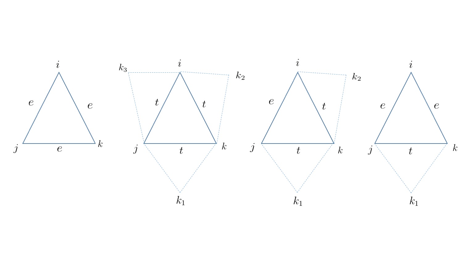
The graph generation process is depicted by an example in Figure 1. Observe that the superimposed graph is allowed to contain multi-edges (or, more precisely, exactly two edges) between two vertices if and only if those vertices are involved in both at least one triangle in and an edge in . A practical justification for this choice of a multi-edge model comes from the fact that pair-wise and triple-wise affinities often provide complementary information222For example, Laniado et al., (2016) studied gender patterns in dyadic and triadic ties in an online social network and found different degrees of gender homophily in different types of ties. Hence instead of duplicating evidence from the same source, we retain two parallel edges in the graph only if they reinforce the information provided by each other.. Clearly, the resulting graph has dependences among its edges and strong local clustering properties for properly chosen matrices due to the increased presence of triangles.
Furthermore, we would like to point out that this inhomogeneous superimposed random graph model differs in a number of important ways from non-uniform hypergraph random graph models on which the non-uniform hypergraph SBM, analyzed by Ghoshdastidar et al., (2017); Chien et al., (2018) and others, is based. First, our model captures networks in which we cannot differentiate between an “ordinary” edge and a hyperedge, as hyperedges simply appear as higher-order structures in the graph. In contrast, the non-uniform hypergraph SBM is a model for networks in which different types of hyperedges are distinguishable during the observation process and labelled. Hence, a major technical difficulty of analyzing methods under the SupSBM is to deal with edge dependencies which are not present in the non-uniform hypergraph SBM. Second, we collapse all multi-edges generated in the hyperedge generation process into single edges which are more realistic as observable network interaction models. We do, however, allow for double edges if there is complementary evidence of both dyadic and triadic ties.
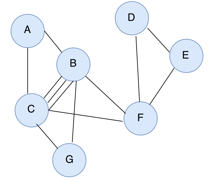

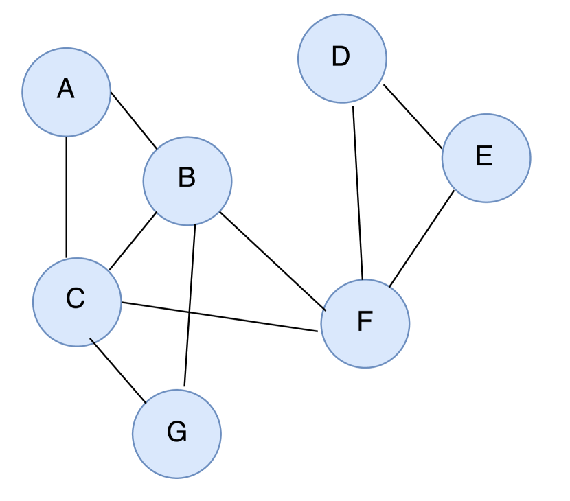

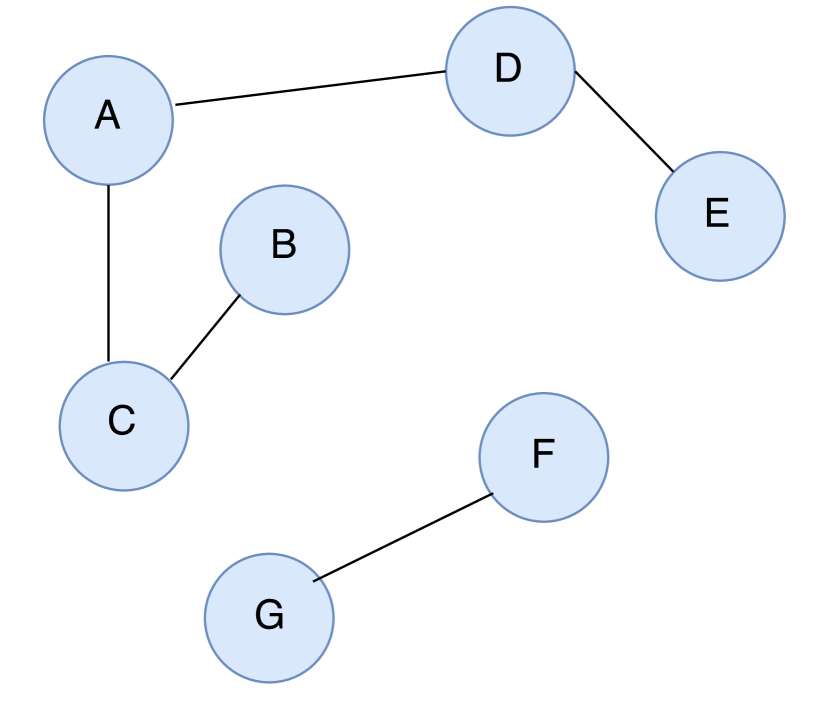

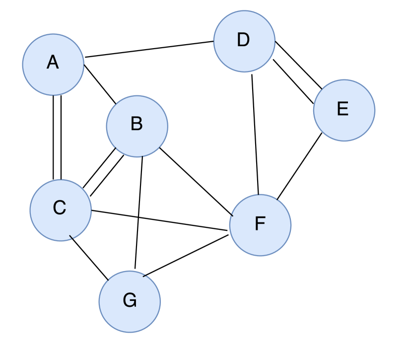
(a) (b) (c) (d)
In the simplest incarnation of the model, one may choose for all and for all . In this case, the graph is a classical Erdös-Rényi dyadic random graph, while before multi-edges collapsing may be thought of as a generalization of Erdös-Rényi graphs to the triadic setting.
We describe next the superimposed stochastic block model based on graphs.
2.1 Superimposed stochastic block models
Our superimposed stochastic block model (SupSBM) is based on the inhomogeneous superimposed random graph framework defined in the previous section. We consider two types of SupSBMs. In the first case, “community signals” are present both in the higher-order structures and the dyadic edges, while in the second case, the “community signals” are present only in the higher-order structures but not in the dyadic edges. Drawing a parallel with the classical SBM, where intra- and inter-community edges are generated via Erdös-Rényi graphs, both the intra- and inter-community edges in SupSBM are generated by superimposed random graph models () as defined in the previous section.
We formally define a graph with vertices and communities generated from a SupSBM as follows. Each vertex of the graph is assigned a community label vector of length , which takes the value of at the position corresponding to its community and at all other positions. To organize the labels, we keep track of an community assignment matrix whose th row is the community label vector for the th vertex. Given the community assignments for all the vertices in the graph, the triangle hyperedge indicators involving three distinct vertices , , are (conditionally) independent, and they follow a Bernoulli distribution with a parameter that depends only on the community assignments, i.e.,
where is a -way tensor of parameters. The triangle hyperedges naturally reduce to a triangle, and as before, multi-edges are collapsed to form the graph .
An edge between two vertices and is generated independently of other edges and hyperedges following a Bernoulli distribution with a parameter that also depends on the community assignments, so that the edge indicator variable satisfies
where is a matrix of model parameters. For the case that the community structure is present only in the higher-order structures and not at the level of dyadic edges, this parameter equals irrespective of the communities that the vertices and belong to. The desired graph is obtained by superimposing and following the process described in the previous section.
The above described model contains a large number of unknown parameters, and to enable a more tractable analysis, we proceed as follows. We define the stochastic block model on hyperedges in the following manner:
so that the probability of a triangle hyperedge equals if the three vertices involved are in the same community, and if at least one of the vertices is in a different community than the other two. The dyadic edges are generated according to the following rule: the probability of an edge is if both the end points belong to the same community and if they belong to different communities.
Another simplification consists in assuming that all communities are of the same size, leading to balanced -vertex -block SupSBMs, , in which all the communities have vertices and the matrix is an community assignment matrix.
3 Analysis of higher-order spectral clustering
Spectral clustering methods for hypergraphs, also known as higher-order spectral clustering methods, have been studied in a number of recent papers (Zhou et al., 2006; Benson et al., 2016; Tsourakakis et al., 2017; Li and Milenkovic, 2017). In particular, Benson et al., (2016) introduced a method that creates a “motif adjacency matrix” for each motif structure of interest. In a motif adjacency matrix, the th element represents the number of motifs that include the vertices and . Spectral clustering is applied to the motif adjacency matrix in a standard form in order to find communities of motifs. While there are many variants of spectral clustering that may be applied to the motif adjacency matrices, throughout our analysis, we investigate only one algorithm, which computes the eigenvectors corresponding to the largest in absolute value eigenvalues of the motif adjacency matrix. The algorithm subsequently performs a -approximate, , -means clustering (Kumar et al., 2004; Lei et al., 2015) on the rows of the resultant matrix of eigenvectors. Furthermore, we only consider two motif adjacency matrices, involving edges and triangles. The primary goal of our analysis is to describe how to detect the community structures of the SupSBM from observed triangle patterns using spectral clustering. We will consider both versions of SupSBM, namely, one with community structure present only at the triangle level, and another with community structure present both at the triangle and edge levels. In what follows, we first prove a number of concentration results for certain motif adjacency matrices under the more general inhomogeneous superimposed random graph model. Subsequently, we specialize our analysis to the SupSBMs.
3.1 Higher-order spectral clustering and superimposed random graphs
Let be a graph generated from the inhomogeneous superimposed edge-triangle random graph model. We introduce two matrices, and , respectively; represent the number of observed edges between the vertices and , while represents the number of observed triangles including both and as vertices. Note these matrices are not the motif adjacency matrices of and , since there are edges in that contribute to and triangles from that contribute to . There may be many “incidentally generated” or imposed triangles (Chandrasekhar and Jackson, 2014) that arise due to superimposition which also contribute to . The different scenarios are depicted in Figure 2. For our analysis, we also introduce the following two matrices:
-
•
: the adjacency matrix of edges in ; here,
-
•
: the adjacency matrix of triangle motifs in ; here,
(a) (b) (c) (d)
As noted in Chandrasekhar and Jackson, (2014), there are four classes of matrices needed to describe the model, namely
-
(a)
: the motif adjacency matrix of all triangles formed by random edges from . The generative random variable for these triangles reads as:
and .
-
(b)
: the motif adjacency matrix of all triangles formed by three intersecting triangles from . The generative random variable for these triangles reads as:
and .
-
(c)
: the motif adjacency matrix of all triangles formed by two triangles from and one edge from . The generative random variable for these triangles reads as:
and .
-
(d)
: the motif adjacency matrix of all triangles formed by one triangle from and two edges from . The generative random variable for these triangles reads as:
and .
Note that except for case (a), an imposed triangle involving the vertices arises only if there is no model-created triangle involving already present. Hence, the definitions of each of the random variables , and include as a factor that indicates this dependence. For case (a), since we allow a multiedge between two vertices that are both involved in a triangle hyperedge and an edge, it is possible to have an imposed triangle in addition to a model-generated triangle on the same triple of vertices.
With these definitions, we have that the triangle adjacency matrix reads as
capturing both model-based and imposed triangles. Obviously, we only observe the matrices and and not their specific constituents, as in real networks we do not have labels describing how an interaction is formed. Hence, even though the community structure is most explicitly described by , we need to analyze how this matrix reflects on and what the properties of the latter matrix are based on . Then, the expectation of equals
where all operators are used component-wise.
3.1.1 Notation and asymptotic properties of superimposed graphs
We start with some notation. Let
denote the maximum probability of edge inclusion in and triangle hyperedge inclusion in respectively. As noted by Chandrasekhar and Jackson, (2014), in the superimposed random graph framework, the generative probabilities summarized in the two matrices and must satisfy certain conditions in order to ensure that the imposed triangles do not significantly outnumber the generative triangles. Accordingly, we impose the following asymptotic growth conditions on and :
| (3.1) |
| (3.2) |
and for some and constants , , and independent of . A typical example are the following two growth rates: and . Note that the asymptotic growth bounds are required only for the analysis of superimposed random graphs under the SupSBM. We do not require these relations to hold for results regarding regular SBMs or 3-uniform hypergraph SBMs. Hence, we will not make any assumptions on the asymptotic growth bounds for and until Theorem 6.
The following five results, summarized in Theorems 1 to 5, provide non-asymptotic error bounds that hold in more general settings, as described in the statements of the respective theorems. Note that we make repeated use of the symbols or to represent different generic constants as needed in the proofs in order to avoid notational clutter.
It is well-known that the Frobenius norm is bounded by with probability at least (Lei et al., 2015; Gao et al., 2015; Chin et al., 2015), where . The following theorems establish similar upper bounds for other component matrices involved in our analysis as well as a bound on . The proofs of all theorems are delegated to the Appendix.
3.1.2 Concentration bounds for
Theorem 1.
Let be a -uniform hypergraph in which each possible 3-hyperedge is generated according to a Bernoulli random variable with parameter independent of all other 3-hyperedges. Let , as before, stand for the triangle-motif adjacency matrix. Furthermore, let . Then, for some constant , there exists a constant such that with probability at least , one has
Note that in the above bound, may be interpreted as being an approximation of the maximum expected “triangle degree” of vertices in . Drawing a parallel with adjacency matrices of graphs, one may define the “degree” of a row of an arbitrary matrix as the sum of the elements in that row. Then, is an upper bound on the degree of a row in the matrix much like is an upper bound for the degrees of the rows in . The above result for triangle-motif adjacency matrices is hence an analogue of a similar result for standard adjacency matrices described in Lei et al., (2015); Gao et al., (2015); Chin et al., (2015). The arguments used to prove the result in the cited papers are based on an net analysis of random regular graphs laid out in Friedman et al., (1989); Feige and Ofek, (2005). We extend these arguments to the case of triangle hyperedges; due to the independence of the random variables corresponding to the hyperedges involved in all sums of interest, we do not require new concentration inequalities to establish the claim. This is not the case for the results to follow.
3.1.3 Concentration bounds for
Next, we derive an upper bound for the spectral norm of the matrix . Note that the elements of the matrix are dependent and consequently, the sums of the random variables used in the net approach include dependent variables. Hence, the net approach cannot be applied directly, and several substantial modifications in the proofs are needed. However, each element of is a low-degree polynomial of the generic independent random variables . Therefore, we show that in all the sums of dependent random variables of our interest, the dependencies between the random variables are limited, and the number of co-dependent random variables are significantly smaller than that of all the variables in the sum. In what follows, we build upon recent advances in concentration inequalities for functions of independent random variables (Warnke, 2016) and sums of dependent random variables (Warnke, 2017) to derive concentration bounds for .
Let , and and assume . We have the following result.
Theorem 2.
Let be an inhomogeneous random graph in which each edge is independently generated by a Bernoulli random variable with parameter . Let for some constant . Then, for some constant , there exists a constant such that with probability at least ,
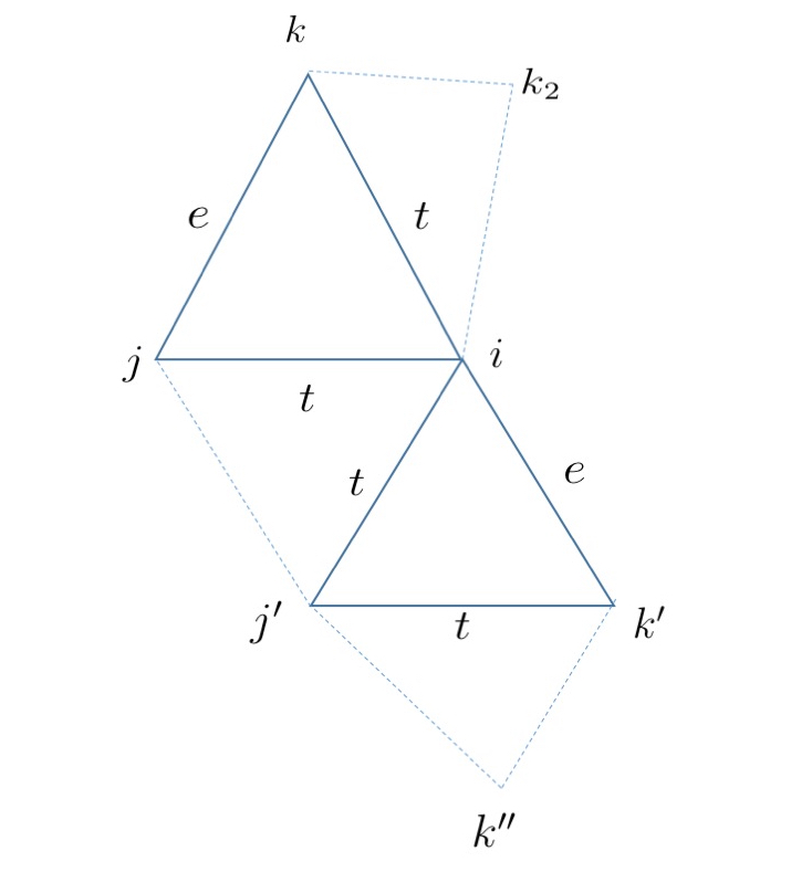
The proof of the result is based on Theorem 1.3 of Warnke, (2016) and Theorem 9 of Warnke, (2017). We still resort to the use of nets but also take into account the particular dependencies between the random variables. The key observations are that two triangles generated by edges from are dependent if they share an edge (see Figure 3(a)), and, with high probability, each triangle shares an edge with at most other triangles. The random variables whose sums we are interested in bounding represent such triangles. Note that our result is a stronger bound than the one actually needed for obtaining an upper bound for under the asymptotic growth conditions of interest. Indeed, Proposition 1 stated in the Appendix automatically gives an upper bound of the form for . While this loose bound would have been sufficient, we resorted to a more careful analysis using the net approach and the results of Theorem 1.3 of Warnke, (2016) to arrive at a significantly improved bound . We also note that based on the results derived for and , the bound for the case when the elements of are mutually independent should read as . The current bound is worse than this bound by a factor of , and it is not immediately clear how the latter bound can be improved further.
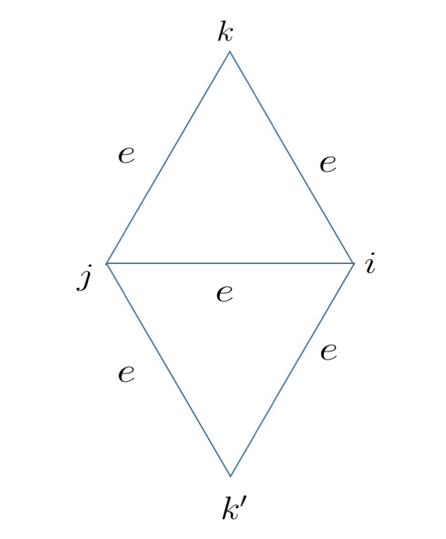
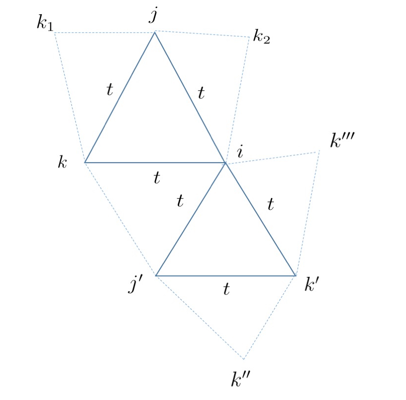
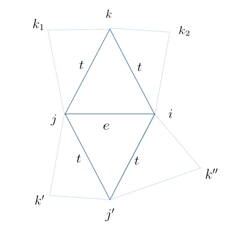
(a) (b) (c)
(d) (e) (f)
3.1.4 Concentration bounds for other relevant matrices
For the next three results, we use the following property of the spectral norm of a square symmetric matrix. For any square symmetric matrix , define the spectral norm of as , the largest singular value of , the 1-norm as , and the norm as . Now assume is an symmetric matrix whose elements are non-negative random variables. Let the entries of its expectation, , also be non-negative. Then,
| (3.3) |
where the first inequality is Corollary 2.3.2 in Golub and Van Loan, (2012), and the second equality follows since is a symmetric matrix by assumption. Note the first term in the final sum is the degree of row of the matrix . Hence, a high-probability bound on the maximum degree will allow us to upper bound this quantity. The second term equals the maximum expected degree of , which is a deterministic quantity. For the next three theorems in this section we assume and .
Theorem 3.
Let be a graph generated by the superimposed random graph model. Let
where is some constant. Then, there exists a constant , such that with probability at least , one has
Theorem 4.
Let be a graph generated by the superimposed random graph model. Let
where is some constant. Then, there exists a constant , such that with probability at least , one has
Theorem 5.
Let be a graph generated by the superimposed random graph model. Let
where is some constant. Then, there exists a constant , such that with probability at least , one has
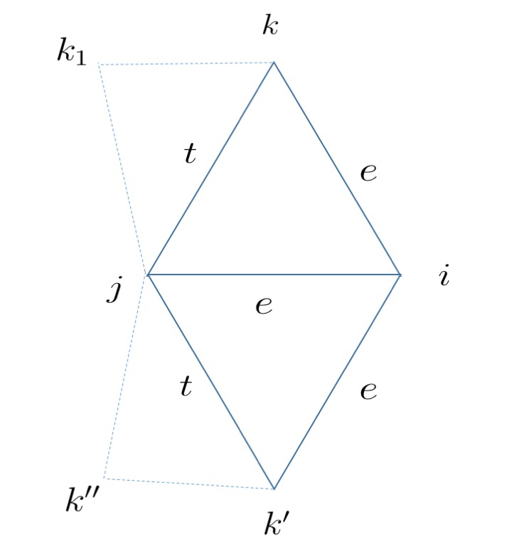
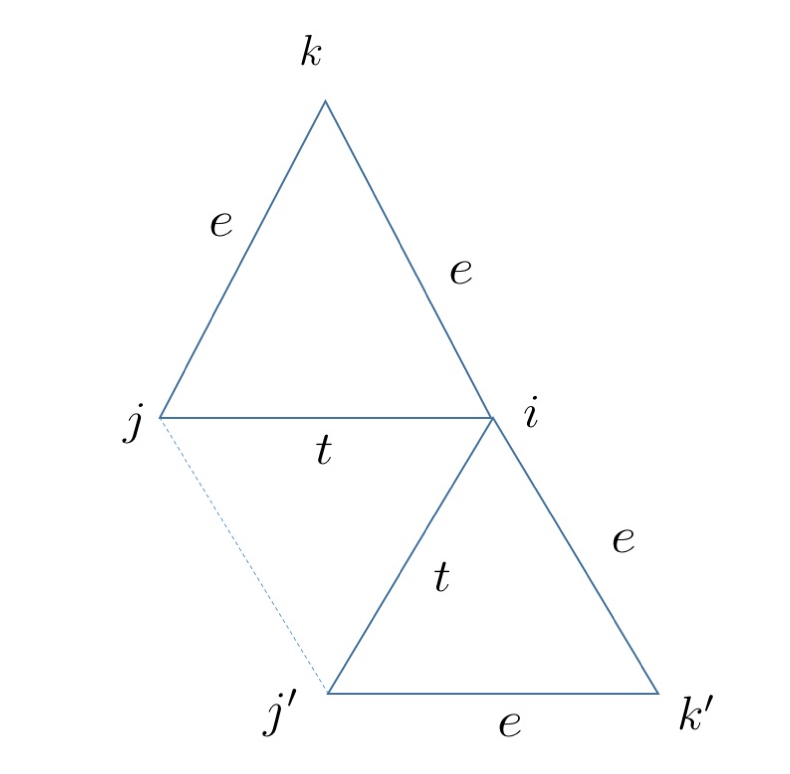
The proofs of all three above results follow a similar outline. In each case, the degree of a row is a sum of dependent triangle-indicator random variables for triangles that include vertex . However, in each case we carefully enumerate the events that lead to two such incidental triangle indicator random variables to be dependent and show that the number of such cases is limited with high probability. This allows us to apply Theorem 9 of Warnke, (2017) in an iterative manner and obtain concentration results on the respective sums. While we relegate technically involved rigorous proofs to the Appendix, we graphically illustrate all the events that lead to the dependencies that we need to consider in Figure 3. For the family of random variables , two variables are dependent if and only if one of the triangles from covering has an edge or and consequently also covers (see Figure 3(b)). For the family of random variables , two variables are dependent if either one of the edges or is covered by a triangle from and the same triangle edge-intersects (see Figure 3(c)), where one of or is an edge in and is also an edge in (see Figure 3(d)). Finally, for the family of random variables , two variables are dependent if either one of the edges or is covered by a triangle from and the same triangle edge-intersects (see Figure 3(e)), or, one of the two edges and is generated by and is also an edge covered by (see Figure 3(f)).
We also note that the bounds in the previous three results can be improved by applying the net approach for dependent random variables as used in Theorem 2. However, the above stated upper bounds suffice to obtain the desired concentration bound for , as summarized in the following subsection.
3.1.5 Concentration bound for
In the next theorem we combine the previous results to arrive at a concentration bound for the matrix under the assumptions made on and in (3.1) and (3.2).
Theorem 6.
We note the similarity of the upper bound of this concentration inequality with that obtained for in Theorem 1. The above result then tells us that the effect of the incidental triangles on the concentration of is limited and the rate in the upper bound is predominantly determined by the rate for . This suggests that while the superimposition process induces dependencies between the edges in through the presence of triangles from , the model, under suitable sparsity conditions, is still mathematically tractable. The influence of the incidental triangles can be analyzed and controlled.
Next, we turn our attention to analyzing random graphs generated by SupSBMs, and focus in particular on quantifying the misclustering error rate under a higher-order spectral clustering algorithm.
3.2 Higher-order spectral clustering under the SupSBM
Let be a graph generated by the balanced -vertex, -block SupSBM with a community assignment matrix as defined before. Let denote the matrix of eigenvectors corresponding to the largest absolute-value eigenvalues of the triangle motif adjacency matrix . To obtain the community assignments for the vertices, a -approximate -means clustering, with , is performed on the rows of (Kumar et al., 2004; Lei et al., 2015).
We define the misclustering error rate as follows. Let and denote the vectors containing the true and estimated community labels of all the vertices in . Then we define
where the infimum is taken over all permutations of the community labels.
To bound the misclustering rate , one needs to relate it to the difference between the estimated and the true eigenvectors. For this purpose, one can use the well-known Davis-Kahan Theorem (Davis and Kahan, 1970; Stewart and Sun, 1990) that characterizes the influence of perturbations on the spectrum of a matrix. For a symmetric matrix , let stand for its smallest in absolute value non-zero eigenvalue. Since
is the matrix of eigenvectors it has orthonormal columns, and hence we have the following bound
| (3.4) |
where is an arbitrary orthogonal matrix (Lei et al., 2015) and the last inequality arises from the Davis-Kahan Theorem.
Next, we derive a lower bound on . We start by computing the expectations of the motif adjacency matrices , , and under the SupSBM. In all three cases, these expectations are of the form , where as before denotes the community assignment matrix, is the -dimensional identity matrix, is the -dimensional vector of all s, and and are functions of the parameters .
For matrices of the form , with , is an eigenvector corresponding to the eigenvalue and the remaining non-zero eigenvalues are of the form where the values of and differ for the different matrices (Rohe et al., 2011). Since , the smallest non-zero eigenvalue equals .
We start by analyzing . Clearly,
so that
Next, we note that the expected value of equals . When , i.e., when the vertices and are in the same community, then
while when
The difference between the two above entities equals
Hence,
Consequently,
| (3.5) |
To determine , we first note that
When ,
while when ,
The difference between the above two probabilities equals
Hence,
Consequently, the smallest non-zero eigenvalue equals
| (3.6) |
A special case of the SBM that is widely analyzed in the literature is the balanced SBM, in which vertices are partitioned into two blocks. In our setting, balancing implies that the SupSBM model of interest has parameters , and it results in and .
We are now ready to state the main result of the paper.
Theorem 7.
Let be a graph generated from the balanced block SupSBM. If then with probability at least , the misclustering rate of community detection using the higher-order spectral clustering method satisfies
Under the assumed growth rate on we have , and hence we can replace by . Under the block balanced SupSBM model, . Hence ignoring the constants, we can rewrite the upper bound as
As an example, if we assume and for constants and , then the result implies that it is possible to detect the communities consistently as long as .
For the special case of a -vertices and -block SupSBM , we can further simplify this upper bound to
| (3.7) |
For comparison, we note that the result in Lei et al., (2015) for the misclustering rate of spectral clustering with classical adjacency matrices under the SBM reads as .
3.3 Uniform and non-uniform hypergraph SBMs
In what follows, we analyze the performance of the higher-order spectral clustering under the uniform and non-uniform hypergraph SBMs (Ghoshdastidar et al., 2017; Chien et al., 2018). The balanced -vertex -block 3-uniform hypergraph SBM is defined in the following way. All the communities have an equal number of vertices , and the probability of forming a triangle hyperedge equals if all three vertices belong to the same community, while the probability of forming a triangle hyperedge equals if one of the vertices belongs to a different community than the other two.
Non-uniform hypergraphs involve two types of hyperedges, edges and triangles, that need to be described separately. Note that this model differs from the superimposed random graph framework used throughout the paper as the observations are of the form of two-way and three-way interactions between entities. Hence, we have a way to differentiate between an edge and a triangle hyperedge. The -vertex -block balanced non-uniform hypergraph SBM is defined in the same way as a SupSBM, except that we do not replace the generated triangle hyperedges with three ordinary edges and we do not collapse multiedges.
If we assume our observed graph is generated from a uniform hypergraph SBM on triangle hyperedges, then spectral clustering of the motif adjacency matrix is equivalent to spectral clustering based on only. Let be the matrix of eigenvectors corresponding to the largest absolute eigenvalues of the matrix . Then, using the bound for in Theorem 1 from Section 3.1.2, we arrive at the following result.
Theorem 8.
Let be a triangle hypergraph generated from the -block uniform triangle hypergraph SBM with parameters . Then, with probability at least , the misclustering rate of the community assignments obtained using the higher-order spectral clustering algorithm applied to the triangle motif adjacency matrix equals
We can simplify this upper bound under the assumption of a -vertex -block triangle hypergraph SBM to Note that the concentration bound is smaller by a factor of when compared to the same result for spectral clustering of ordinary edge-adjacency matrix in Lei et al., (2015), provided that the parameters and are comparable. Alternatively, the misclustering error rate using the triangle motif adjacency matrix for a graph generated from a triangle hypergraph SBM is better than the corresponding rate from an edge-based adjacency matrix of a graph generated from SBM as long as .
The above observation has important implication for non-uniform hypergraph SBMs. To describe why this is the case, assume that we are given a non-uniform hypergraph generated from the -vertex -block balanced non-uniform hypergraph SBM The question of interest is: Given , with and , should one use the edge-based adjacency matrix, the triangle-based adjacency matrix, or a combination thereof? Let
| (3.8) |
so that asymptotically, the probabilities and are -times the probabilities and , while the difference between the probabilities is times that of the difference between . Clearly, captures the asymptotic difference between the densities of triangle hyperedges and dyadic edges, while captures the difference in the “communal” qualities between these two types of hyperedges. Note that the notation for asymptotic equivalence ignores all constants.
Theorem 9.
Let be a graph generated from the non-uniform hypergraph SBM. Assume the relationships between the probabilities are as in Equation (3.8). Then, spectral clustering based on a triangle adjacency matrix has a lower error rate than spectral clustering based on an edge adjacency matrix if and a higher error rate if .
Note that even though in practice we do not observe the quantities and , it is possible to estimate them reliably and efficiently. To estimate , we only need to look at the ratio of the densities of the hyperedges. The expected degree density of triangle hyperedges is , while that of edges is . This implies that
Hence is a “good” estimator of . To obtain an estimate of , we first cluster the vertices using spectral clustering on edges and triangles separately, and then compute the respective probability parameters for intra- and inter-cluster connections. Then, we may use as an estimate of .
The above results also allow us to bound the error rate of spectral clustering of a weighted motif adjacency matrix under the non-uniform hypergraph SBM. Let be the weighted sum of adjacency matrices of edges and triangle hyperedges with known relative weight . Clearly, and the smallest non-zero eigenvalue of is . Then, with probability at least we have
and the error rate is upper bounded according to,
When the asymptotic relationships of Equation (3.8) hold, we can further simplify this expression to
| (3.9) |
While Theorem 9 suggests that depending upon the values of , either the edge-based or triangle-based adjacency matrix has a lower error rate, in practice it might be beneficial for numerical stability to use a weighted average of both of them. The result in Equation 3.9 provides a bound for any weighted sum of these two hyperedge adjacency matrices.
3.4 The classical SBM
For the case of a classical SBM, we are only presented with but not . In this case, is the adjacency matrix of the graph , which we denoted by . The matrix is the triangle motif adjacency matrix constructed from the triangles that arise due to , which we denoted by . The smallest non-zero eigenvalue of equals . In Equation (3.6) we described the smallest non-zero eigenvalue for .
Let and denote the matrices of eigenvectors corresponding to the largest in absolute value eigenvalues of the classical edge-based adjacency matrix and the triangle-adjacency matrix, respectively. Using the bound for from Theorem 2, Section 3.1.3, and the Davis-Kahan Theorem we have the following result.
Theorem 10.
Let be a dyadic graph generated from the -block balanced SBM with parameters . Then, with probability at least , the misclustering rate of the community assignments obtained by higher-order spectral clustering equals
For the case which is a widely analyzed setting in the SBM literature, one can simplify the bound above. First, note that in this case simplifies to , while . Furthermore, since , we have . Thus,
| (3.10) |
We conclude this section by evaluating the performance of spectral clustering on the weighted sum of the two motif adjacency matrices, the edge-based matrix and the triangle-based matrix . For this purpose, let be the weighted sum of motif adjacency matrices, where is a known weight. Clearly, . Then, from the results of Theorem 2 and Theorem 5.2 of Lei et al., (2015), we have that with probability at least , it holds that
The smallest non-zero eigenvalue of can be computed as
From Equation (3.4), we have
3.5 Remarks
Let us start by comparing the upper bound for higher-order spectral clustering under the SBM obtained in Equation (3.10) with the corresponding upper bound for spectral clustering based on the edge-based adjacency matrix , which reads as (Lei et al., 2015). The bound based on the triangle motif adjacency matrix is essentially equal to the bound based on the edge adjacency matrix as long as , or equivalently, as long as . However, when grows slower than this rate, the performance guarantees for spectral clustering based on the motif adjacency matrix is worse than the corresponding bound based on the edge adjacency matrix. This result is intuitively justified as we expect very few triangles in a sparse dyadic graph. The presence of a triangle is a random phenomenon rather than an indicator of community structure. Hence, using triangles for community detection could lead to unwanted errors unless the graph is dense. For , we say that the graph is “triangle-dense” and in this case one can use the triangle-adjacency matrix for community detection. When this condition is not satisfied, we either need to perform some form of regularization or completely dispose of the triangle based adjacency matrix.
However, as previously observed, real world networks contain more triangles and higher-order structures, and consequently have a higher level of local clustering than one would expect from the SBM. Hence, the SupSBM is a more appropriate model for networks with community structures. The upper bound on the misclustering rate in Equation (3.7) suggests that spectral clustering based on higher-order structures can consistently detect communities under the SupSBM. In fact, if , then the underlying upper bound is smaller by a factor of compared to that of the spectral clustering under the standard SBM. This suggests that even though spectral clustering based on higher-order structures may not be appropriate for the SBM, it offers improved performance for the SupSBM. Note that as we focus on higher-order structures based spectral clustering, we did not analyze edge-adjacency matrix based spectral clustering under the SupSBM. We hence cannot compare the misclustering rate of spectral clustering on the triangle-adjacency matrix with that of the edge-adjacency matrix under SupSBM, as the later does not follow directly from the existing results, e.g., Lei et al., (2015) (due to the fact that the observed edge-adjacency matrix has edges generated by triangles from in addition to edges from ). Nevertheless, our analysis of the non-uniform hypergraph SBM, especially Theorem 9, describes the error rate tradeoff between spectral clustering with edge-based and triangle-based adjacency matrices.
4 Experiments on Real Data
We test the effectiveness of spectral clustering using a weighted sum of adjacency and Laplacian matrices for higher-order structures on three benchmark network datasets. In particular, we choose to work with a uniformly weighted edge-triangle adjacency matrix, , where and are the observed edge and triangle adjacency matrices defined earlier. The normalized Laplacian matrix is obtained as , where is a diagonal matrix such that . We compare the performance of various known forms of spectral clustering methods based on edge-based matrices, namely those using adjacency matrices (spA), normalized Laplacian matrices (spL), and regularized normalized Laplacian matrices (rspL) (Sarkar et al., 2015; Chin et al., 2015; Qin and Rohe, 2013) with their weighted higher-order structure counterparts, hospA, hospL and horspL, respectively. In all six instances of the spectral clustering, the eigenvectors are row-normalized before applying the k-means algorithm. Table 1 summarizes the performance of the methods.
Political blogs data. The political blog datasets (Adamic and Glance, 2005), collected during the 2004 US presidential election, comprise political blogs with hyperlinks between them, giving rise to directed edges. These benchmark datasets have been analyzed by a number of authors (Karrer and Newman, 2011; Amini et al., 2013; Qin and Rohe, 2013; Joseph and Yu, 2016; Jin, 2015; Gao et al., 2017; Paul and Chen, 2016) in order to test community detection algorithms. Following previous approaches, we first convert directed edges into undirected edges by assigning an edge between two vertices if there is an edge between them in either direction and consider the largest connected component of the resultant graph which contains vertices. The ground truth community assignment used for comparisons splits the graph in two groups, liberal and conservative, according to the political leanings of the blogs. We note the hospA and horspL are competitive with the corresponding edge based methods spA and rspL, respectively. However, for spectral clustering based on the normalized Laplacian matrix, the edge-based method spL completely fails to detect the community structure due to well-documented reasons described in Qin and Rohe, (2013); Jin, (2015); Joseph and Yu, (2016); Gao et al., (2017). On the other hand, hospL succeeds in splitting the graph into two communities with only misclustered vertices.
| Dataset | spA | hospA | spL | hospL | rspL | horspL |
|---|---|---|---|---|---|---|
| Political blogs | 63 | 71 | 588 | 59 | 64 | 64 |
| Karate club | 0 | 0 | 1 | 0 | 0 | 0 |
| Dolphins | 2 | 2 | 2 | 1 | 2 | 1 |
Karate club data. The Zachary’s karate club data (Zachary, 1977) is another frequently used benchmark dataset for network community detection (Newman and Girvan, 2004; Bickel and Chen, 2009; Jin, 2015). The network describes friendship patterns of members of a karate club and the ground truth splits club members into two subgroups. The method spL misclusters one vertex, while all other methods manage to recover the communities in an error-free manner.
Dolphin social network data. This dataset describes an undirected social network involving dolphins in Doubtful Sound, New Zealand, curated by Lusseau et al., (2003). Over the course of the study the group split into two due to departure of a “well connected” dolphin. These two subgroups are used as the ground truth. From Table 1, one can see that only hospL and horspL miscluster one dolphin, while all the remaining methods miscluster two dolphins.
5 Conclusion and future directions
We proposed and analyzed a superimposed stochastic block model, a mathematically tractable random graph model with community structure, that produces networks with properties similar to that observed in real networks. In particular it can generate sparse networks with short average path length (small-world), strong local clustering, and community structure. To produce the strong local clustering property, the model allows for dependencies among the edges, yet remaining mathematically suitable for analysis of algorithms. While not pursued here, a degree correction to the model similar to that of degree corrected stochastic block model is expected to produce networks with highly heterogeneous degree distribution (power law), hub nodes and core-periphery structure while simultaneously retaining the aforementioned properties. We hope to extend the model in that direction in a future work.
We have also analyzed the performance of the higher-order spectral clustering algorithm under the proposed SupSBM. This analysis showed that it is possible to mathematically analyze community detection algorithms under the supSBM, and that the method can detect community structure consistently for graphs generated from the SupSBM. In future, we hope to determine minimax rates of error of community detection under the SupSBM and obtain algorithms that achieve those rates.
Appendix A
In the Appendices we will use and to represent generic constants whose values will be different for different results.
Proof of Theorem 1
Proof.
We follow and extend the arguments in the proof of a similar result for standard adjacency matrices in Lei et al., (2015); Gao et al., (2017), and Chin et al., (2015) to the case of triangle-motif adjacency matrices. The arguments in all of the above mentioned papers rely on the use of nets on random regular graphs (Friedman et al., 1989; Feige and Ofek, 2005).
Let denote the unit sphere in the dimensional Euclidean space. An net of the sphere is defined as follows:
where denotes the set of integers. Hence, is a set of grid points of size spanning all directions within the unit sphere. For our analysis we only use nets of spheres and henceforth use to denote such nets.
Next, we recall Lemma 2.1 of Lei et al., (2015) which established that for any , one has . Hence, a constant-approximation upper bound for may be found by optimizing over all possible pairs . In addition, note that
| (5.1) |
We now divide the pairs into two sets, the set of light pairs and the set of heavy pairs , according to
where is as defined in the statement of the theorem.
We bound the term separately for the light and heavy pairs, as summarized in the following two lemmas.
Lemma 1.
(Light pairs) For some constant , there exists a constant , such that with probability at least ,
Whenever clear from the context, we suppress the dependence of the constants on other terms (e.g., .)
To obtain a similar bound for heavy pairs, we first note that
| (5.2) |
The second term can be easily bounded as follows:
How to bound the first term is described in the next Lemma 2.
Lemma 2.
For some constant , there exists a constant such that with probability at least , .
Combining the results for the light and heavy pairs, we find that with probability at least ,
This completes the proof of Theorem 1. ∎
Proof of Theorem 2
Proof.
As before, we create an net for the unit sphere and separately analyze the light and heavy pairs. In this setting, the pairs are defined according to
and
with as defined in the statement of the Theorem.
For the light pairs, we can prove the following result.
Lemma 3.
(Light pairs) For some constant , there exists a constant such that with probability at least ,
To bound the contribution of the heavy pairs, we once again divide the sum into two terms.
First, let and note that . Then,
| (5.3) |
The second term can be bounded as follows:
where the penultimate inequality follows since if , then
In addition, if , then . Consequently,
For the first term in Equation (5.3) we have the following result.
Lemma 4.
For some constant , there exists a constant such that with probability at least , .
Combining the results for the light and heavy pairs, we obtain
∎
Proof of Theorem 3
Proof.
The proof of this result and those of Theorems 4 and 5 will repeatedly use Theorem 9 of Warnke, (2017), which we reproduce here for ease of reference.
Proposition 1 (Theorem 9 of Warnke, (2017)).
Let be a collection of non-negative random variables with . Assume that is a symmetric relation on such that each with is independent of . Let , where the maximum is taken over all sets such that . Then for all we have
For any vertex , define the degree of in the matrix according to
The expectation of the degree may be bounded as
where the second inequality follows since
Let denote the set of all triangles incident to vertex and generated incidentally by three other triangles in . Observe that the set comprises elements that are indicator random variables indexed by corresponding to incidentally generated triangle. Consequently, two random variables in the family , when restricted to the set , are dependent if and only if one of the triangles creating the edges or of includes or as a vertex and is consequently part of (see Figure 3(b)). We refer to an event corresponding to the above described scenario as and note that this event also accounts for the case when we have “sharing” the edge with .
In summary, the set contains dependent random variables, with denoting the sum of all the random variables in the set . However, in what follows we show that the dependence is “limited” in the sense that we can limit the number of other variables dependent on one random variable in the set to with high probability.
We characterize the event through an associated indicator random variable. We show that the number of incidentally generated triangles that give rise to TC events is bounded, provided that certain “good events” occur with high probability. For this purpose, let be a triangle in leading to the creation of an incidental triangle (see Figure 3(b)). To create the incidental triangle , we also require the existence of at least two triangles from with edges and . We capture this event through its indicator variable
Observe that one can think of , as the random variable given that (see Figure 3(b)). Consequently, for any , the number of incidentally generated triangles that also belong to the set and contribute to the occurrence of the event is at most .
Next, we define a “good event” as , where and are two events that for any may be described as follows:
Hence, the event essentially asserts that there are choices for the value of , and given a , the event asserts that there are choices for a . Consequently, under the “good event” the number of triangles in on which a triangle depends on is .
Next, define a set as follows:
In a nutshell, the sets are collections of ’s such that no is dependent on more than other ’s. Let state that the two underlying random variables indexed by and are dependent. Then we have,
Applying Proposition 1 for leads to
The last inequality may be established through the following argument. If , then , which implies
Then, , and consequently
On the other hand, if , then . Now, either , in which case and . Or, , and consequently . Then
since by assumption.
Recall that the event describes the only setting for which two random variables in the set are dependent on each other; under the good event , we have and consequently, .
Next, we need to show that the probability of the “bad event” (i.e., complement of the good event) is exponentially small. For that, we note
The last term can be easily bounded using Bernstein’s inequality as follows. Let . Then counts the number of triangles in sharing an edge . The event asserts that the number of triangles in sharing an edge is at most . From Bernstein’s inequality and the union bound we consequently have
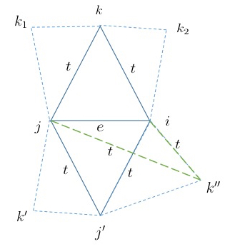
(a) (b)
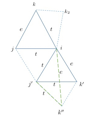
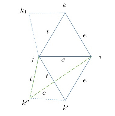
(c) (d)
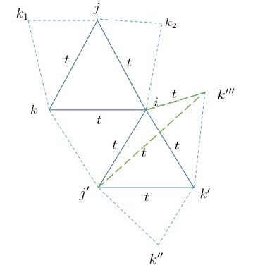
We now turn our attention to the event . Fix a . The sum includes dependent random variables; two random variables in the sum, say and , are dependent if and only if there is a triangle, say in that has both and as edges (Figure 4(a)). However, the number of triangles in sharing an edge can be bounded by referring to the event . First, we define to be the collection of all with fixed and . Then, we define the sets s as subsets of such that no is dependent on more than other s. To apply Proposition 1 to , we first observe that one may upper bound the relevant expectation as
and Then, with ,
The last inequality holds due to the following argument. If , then , and consequently, . Then . If , then since . Since there are at most choices for , for any , the union bound leads to
Combining the results we have
Invoking the union bound, now over all , we can show that with probability at least . By Equation (3.3), the claimed result holds. ∎
Proof of Theorem 4
Proof.
Triangles of type are generated by two triangles from and one edge from . Without loss of generality, we may assume that in , the sides and are generated by triangles from and that the side is generated by an edge from . Then, we have
Let the set denote the set of all incidentally generated triangles of type that includes the vertex . The set , indexed by , represents a family of indicator variables corresponding to incidentally generated triangles of type . Two random variables in the family restricted to the set may be dependent in two scenarios. One possibility is that one of the sides or is an edge from and serves as an edge for or for some (see Figure 3(c)). The other possibility is that one of the sides or is created by a triangle from and the same triangle is involved in creating for some and (see Figure 3(d)). We refer to these two events as and , respectively.
We now need to derive a bound on , which equals the sum of the random variables , that holds with high probability. We proceed as in the proof of the previous theorem and describe “good events” which limit the number of random variables that a random variable in the sum depends on with high probability.
For this purpose, we characterize the events and using indicator variables. First, define the random variables
Then, for any , the number of other incidentally generated triangles in creating the event is at most (Figure 3(c)).
With regards to the event , define the following random variable
Then, for any , the number of additional incidental triangles in that contribute to the event is at most (Figure 3(d)).
As before, define a “good event” as , where for any , , and are defined as:
Note the second event is the same as the event described in the proof of Theorem 3.
As in the previous setting, the events above are defined in a way that ensures that “good events” happen with high probability. We note that under the events and , one has
Hence, the two events limit the number of occurrences of the events and , respectively, and consequently limit the number of random variables that a random variable in the sum is dependent on. We once again apply Proposition 1 to under the good event to obtain an upper bound for . For this purpose, define a set as follows:
where may be found from
Then, , and with ,
where the last inequality holds due to the following argument. If , then which, by assumption, is greater than . If , then which, by assumption, is greater than . Finally, if then .
In our previous proofs, we already established upper bounds for and . To complete the proof of the claimed result, we only need to determine an upper bound on . Using the previously introduced variables , the event occurs if for any . Note that the sum includes dependent random variables.
An upper bound on the expectation of this sum reads as
We also introduce the set that restricts the number of -variables that another -variable in the sum is dependent on:
Fix and and define to be the collection of all random variables that contribute to the event . Two random variables in the sum , say and , are dependent (conditioned on ) if and only if the triangle from generates an edge for both the incidental triangles characterized by and (see Figure 4(c)). The set essentially limits the frequency of such triangles s: under the event , the largest set as defined above is equal to the set . We therefore have , and for ,
where the last inequality follows since if , then which, by assumption, is greater than ; and, if , then . Combining the previous results we obtain
Applying the union bound over all indices we can bound with probability at least . Then, from Equation (3.3) we arrive at the result claimed in the theorem. ∎
Proof of Theorem 5
Proof.
For incidental triangles of type , the generating class is one triangle from and two edges from . Consequently, we have
Next, let denote the set of all incidentally generated triangles of type including a vertex . Then, indexed by is a family of indicator variables with each variable corresponding to an incidentally generated triangle of type . Two different random variables in the family restricted to the set may be dependent in two ways. First, one of the edges or of the incidental triangle characterized by , may be an edge from and be an edge in the incidental triangle characterized by for some (see Figure 3(e)). Second, one of the edges or may have been created by a triangle from , with the same triangle being involved in creating the incidental triangle characterized by for some and (see Figure 3(f)). Note the second possibility also includes the case when the triangles characterized by and share an edge which is created by a triangle from . We refer to these two events as and , respectively.
With regards to the event , define the following random variable
Conditioned on , each characterizes an incidentally generated triangle in and contributes to the event ; for simplicity, we let stand for the set of all such variables . Then, for any , the number of additional incidentally generated triangles in contributing to the event is at most (Figure 3(e)).
With regards to the event , define the random variable
Conditioned on , each characterizes an incidentally generated triangle in and leads to the event ; for simplicity, we let stand for the set of all such variables s. Then, for any , the number of additional incidentally generated triangles in contributing to the event is at most (Figure 3(f)).
Define a “good event” as , where for any , , and may be described as follows:
We again apply Proposition 1 to under the good event to obtain an upper bound on .
Under the event , it holds that which in turn implies that the number of in that depend on according to the event is limited to . Furthermore, for the event , we have which implies that the number of in that depend on according to the event is limited to .
Now, define a set as follows:
where may be found according to
Then, for ,
where the last inequality follows since if , then which is by assumption greater than ; if , then ; and if , then . Finally, if then .
We bounded the probability in the previous proof, while a bound on is given in Lemma 3.
Combining the expressions for all previously evaluated bounds, we obtain
Taking the union bound over all , we can show that holds with probability at least . The claimed result then follows from Equation (3.3). ∎
Proof of Theorem 6
Proof.
We note that under the given assumptions on and we have the following results:
Consequently,
where is the maximum of all constants used for bounding the individual matrix terms, and is another constant that may be easily computed from the previous inequalities. ∎
Proof of Theorem 7
Proof.
First, note that and all matrices in the sum under the SupSBM model may be written in the form . Consequently can also be written in the form . Then, we have for some and . Now note that the term in is the sum of the corresponding terms in the component matrices, all of which are positive due to the community structure of the SupSBM. Hence, the term of is going to be greater than the term of , so that . This implies that we can replace with in the upper bound of Equation (3.4). We have already computed in Equation (3.5) and the numerator of Equation (3.4) has been upper bounded in Theorem 6. Combining the results, we arrive at the claimed result. ∎
Proof of Theorem 8
Proof of Theorem 9
Proof.
We have the following asymptotic relationship between the two error rates:
Hence, the error rate obtained by using the information about edges is times that of using triangles. Consequently, the error rate is lower for triangle hyperedges if and higher otherwise. ∎
Proof of Theorem 10
Appendix B
Proof of Lemma 1.
Proof.
Define for all . Then,
Note that each term in the above sum is a zero-mean random variable bounded in absolute value, . By applying Bernstein’s inequality we have
where the third inequality follows as a consequence of two observations. First, since , we have
Second,
From Lemma 5 in Vershynin, (2010) regarding the covering number of a sphere, we have . Hence, taking the union bound over all possible and we obtain
The claimed result now follows from selecting a sufficiently large constant and . ∎
Proof of Lemma 2.
Proof.
We first address the subset of heavy pairs . The other cases may be analyzed similarly.
Define the following two families of sets:
Next, for two arbitrary sets and of vertices, also define
Finally, let , , , , and .
We have the following two results establishing relationships between the previously introduced entities.
Lemma 5.
Let denote the triangle-degree of vertex . Then, for all , and a constant , there exists a constant such that with probability at least .
Lemma 6.
For a constant , there exists constants such that for any pair of vertex sets such that , with probability at least , at least one of the following statements holds:
(a)
(b)
Now, we use the result of the two previous lemmas to complete the proof of the claimed result for the heavy pairs. We note
We would like to bound the right-hand-side of the inequality by a constant multiple of . To this end, first note the following two facts:
Following the approach of Lei et al., (2015) and Chin et al., (2015), we split the set of pairs into six parts and show that desired invariant for each part is bounded.
-
•
:
-
•
:
Sinceconsequently
- •
- •
-
•
:
First, note that since , we have and hence . Next, and hence . Therefore, -
•
:
Since , we have . This observation, along with the fact , implies that . As a result,
In a similar fashion, the set of pairs is split into six categories in order to bound . The derivations are omitted.
Collecting all the previously obtained terms, we arrive at the claimed result for heavy pairs: for some constant , there exists a constant such that with probability at least , one has
∎
Proof of Lemma 3
Proof.
As before, define for all . Then,
To analyze the above sum, we use the typical bounded differences inequality of Theorem 1.3 in Warnke, (2016). For this purpose, define
Clearly, is a low-order polynomial of independent random variables. More precisely, since are independent Bernoulli random variables with parameters , we have
Let be the number of common neighbors of the vertices and , i.e., . Then is a sum of independent Bernoulli random variables with parameters . Next, define a “good set” under which the contribution of one single random variable to the function is limited with high probability as follows:
asserting that every pair of vertices has at most common neighbors. From Bernstein inequality we have,
where the last inequality holds since by definition. Observe that the good event is independent on the particular values of .
Next, we determine the typical Lipschitz (TL) condition for the function . Changing one element in the sequence (say, ) from to may have two different types of effects on . The effect may be “large” on the term , which is upper bounded by . Or, the effects may be “small” for the terms of the form and (i.e., the terms that involve the entries of the matrix which represent neighboring edges of ). These “small” effects are upper bounded by and , respectively.
Under the good event , we have , and consequently, the “large” effect of changing from 1 to 0 is bounded by . Moreover, under the good event , there are at most “small” effects, since for a “small” effect to occur, both and must be 1, i.e., and must be connected by an edge. However, an additional complication is that the effects contribute differently to the bound, depending upon which common neighbor we are looking at. To mitigate this problem, we first lump the “small” effects together into . Combining the “large” and “small” effects, under the good event,
emerges as an upper bound on the total effect of changing one in . For the case that the bad event occurs instead, an upper bound on the effect of the change is .
Now, let for all . Then , and
Next, we need to compute an upper bound on . This can be done as follows
Within the sum of over all , each term will appear at most times. This implies that .
In the notations of Theorem 1.3 of Warnke, (2016) define for all and the event , such that and
Then using Theorem 1.3 of Warnke, (2016), we have
where the penultimate inequality follows since .
Clearly, the event does not depend on the choice of the vectors . Hence, taking the supremum over all and , we have
This completes the proof. ∎
Proof of Lemma 4
Proof.
As before, we first focus on the subset of heavy pairs, ; the other two cases follow similarly. The vertex sets are defined as before. In addition, we write
The degree of row of the matrix is . Hence, counts the number of triangles incident to the vertex . Let . Then may be vaguely interpreted as being the (approximate) maximum degree of the rows of the matrix. The next lemma bounds the degrees of the rows of the matrix with high probability.
Lemma 7.
If , then for a constant , there exists a constant such that the “degree” of row , with probability at least for all .
Lemma 8.
For a constant , there exist constants such that with probability at least and for any vertex sets and one of the following two statements is true:
(a)
(b)
We use the result of the two previous lemmas to establish the proof for heavy pairs. In this setting, note that
Next, we need to bound this quantity by a constant multiple of . Following the approach of Lei et al., (2015) and Chin et al., (2015), we split the set of pairs into six parts and show that the contribution of each part is bounded accordingly. Again, in our proof we rely on two facts,
-
•
:
-
•
:
Under , , and consequently,This implies
- •
-
•
:
From part (b) of Lemma 6, we haveNoting that , we may write
Then,
where the penultimate inequality relies on the fact that , and that consequently .
-
•
:
First, note that since , we have and hence . Furthermore, . Since , we have andThen,
-
•
:
Since , we have . This fact, along with implies that . Therefore,
The set of pairs may be similarly split into six categories categories and similar arguments may be used to bound each of the contributions . Collecting all the terms we have the following result for heavy pairs: for some constant , there exists a constant such that with probability at least , one has
∎
Proof of Lemma 5.
Proof.
We note is a sum of independent random variables, each bounded in absolute value by 1. Therefore, Bernstein’s inequality gives
where the last inequality follows since . Taking the union bound over all values of we obtain that with probability at least where is a function of the constant . ∎
Proof of Lemma 6.
Proof.
If , let . We next invoke Corollary A.1.10 of Alon and Spencer, (2004), described below.
Proposition 2.
For independent Bernoulli random variables and , we have
Proof of Lemma 7
Proof.
We use Proposition 1. Let us start with the observation that
Furthermore, let be the set of all triangles of type incident to a vertex . Let , indexed by denote a family of indicator random variables. Define a “good event” as before: under the good event, every pair of vertices has at most common neighbors. Clearly, two triangles belonging to the set are independent if they do not share any edges. For simplicity, let “” denote a relation such that holds if and share an edge. For any , the good event restricts the number of triangles of type in the set that are dependent on to .
Define as
Then, we have
For the above results imply
where the last inequality is a consequence of the following argument. If , then by assumption, and if , then . Under the good event , we have and consequently, . Then,
since . Taking the union bound over all values of results in with probability at least . ∎
Proof of Lemma 8
Proof.
We first note that and .
Next, if , then the result of Lemma 7 implies that
so that in this case (a) holds true. If , define as the set of all -tuples such that each tuple has one vertex in each of the sets and .
To prove that the second statement also holds, we cannot invoke the exponential concentration inequality used in the proof of Theorem 1 due to the lack of the independence assumption. Instead, we use Proposition 1 on the set of -tuples.
First, note that
and
Define to be such that any , for some , depends only on other s. We then have .
Next, let . Then, for some ,
For a constant , define according to
and let . From the previous calculations, we have
Following an identical argument as described in Lei et al., (2015), we have
Therefore, with probability at least , we have . For pairs such that , we readily have
This establishes that part (a) of the claim is true. For the remaining pairs for which holds, we have , and
implying that part (b) of the claim is true as well. ∎
Acknowledgement
The authors would like to thank Prof. Lutz Warnke of Georgia Institute of Technology for explaining how his work may be applied in parts of the analysis. We also appreciate his generous assistance with proving some of the results. The work was supported by the NSF grant CCF 1527636, the Center of Science of Information NSF STC center, and an NIH U01 grant for targeted software development.
References
- Abbe and Sandon, (2015) Abbe, E. and Sandon, C. (2015). Community detection in general stochastic block models: Fundamental limits and efficient algorithms for recovery. In IEEE 56th Annual Symposium on Foundations of Computer Science (FOCS), pages 670–688. IEEE.
- Adamic and Glance, (2005) Adamic, L. A. and Glance, N. (2005). The political blogosphere and the 2004 US election: divided they blog. In Proceedings of the 3rd International Workshop on Link Discovery, pages 36–43. ACM.
- Alon and Spencer, (2004) Alon, N. and Spencer, J. H. (2004). The Probabilistic Method. John Wiley & Sons.
- Alon, (2007) Alon, U. (2007). Network motifs: theory and experimental approaches. Nature Reviews Genetics, 8(6):450–461.
- Amini et al., (2013) Amini, A. A., Chen, A., Bickel, P. J., and Levina, E. (2013). Pseudo-likelihood methods for community detection in large sparse networks. The Annals of Statistics, 41(4):2097–2122.
- Angelini et al., (2015) Angelini, M. C., Caltagirone, F., Krzakala, F., and Zdeborov, L. (2015). Spectral detection on sparse hypergraphs. In 2015 53rd Annual Allerton Conference on Communication, Control, and Computing (Allerton), pages 66–73. IEEE.
- Barabási and Albert, (1999) Barabási, A.-L. and Albert, R. (1999). Emergence of scaling in random networks. Science, 286(5439):509–512.
- Battiston et al., (2017) Battiston, F., Nicosia, V., Chavez, M., and Latora, V. (2017). Multilayer motif analysis of brain networks. Chaos: An Interdisciplinary Journal of Nonlinear Science, 27(4):047404.
- Benson et al., (2016) Benson, A. R., Gleich, D. F., and Leskovec, J. (2016). Higher-order organization of complex networks. Science, 353(6295):163–166.
- Bickel and Chen, (2009) Bickel, P. J. and Chen, A. (2009). A nonparametric view of network models and Newman–Girvan and other modularities. Proceedings of the National Academy of Sciences, 106(50):21068–21073.
- Bollobás et al., (2007) Bollobás, B., Janson, S., and Riordan, O. (2007). The phase transition in inhomogeneous random graphs. Random Structures & Algorithms, 31(1):3–122.
- Bollobás et al., (2011) Bollobás, B., Janson, S., and Riordan, O. (2011). Sparse random graphs with clustering. Random Structures & Algorithms, 38(3):269–323.
- Boucheron et al., (2013) Boucheron, S., Lugosi, G., and Massart, P. (2013). Concentration Inequalities: A Nonasymptotic Theory of Independence. Oxford university press.
- Celisse et al., (2012) Celisse, A., Daudin, J. J., and Pierre, L. (2012). Consistency of maximum-likelihood and variational estimators in the stochastic block model. Electronic Journal of Statistics, 6:1847–1899.
- Chandrasekhar and Jackson, (2016) Chandrasekhar, A. and Jackson, M. O. (2016). A network formation model based on subgraphs. arXiv preprint arXiv:1611.07658.
- Chandrasekhar and Jackson, (2014) Chandrasekhar, A. G. and Jackson, M. O. (2014). Tractable and consistent random graph models. Technical report, National Bureau of Economic Research.
- Chien et al., (2018) Chien, I., Lin, C.-Y., and Wang, I.-H. (2018). Community detection in hypergraphs: Optimal statistical limit and efficient algorithms. In International Conference on Artificial Intelligence and Statistics, pages 871–879.
- Chin et al., (2015) Chin, P., Rao, A., and Vu, V. (2015). Stochastic block model and community detection in sparse graphs: A spectral algorithm with optimal rate of recovery. In COLT, pages 391–423.
- Choi et al., (2012) Choi, D. S., Wolfe, P. J., and Airoldi, E. M. (2012). Stochastic blockmodels with a growing number of classes. Biometrika, 99:273–284.
- Davis and Kahan, (1970) Davis, C. and Kahan, W. M. (1970). The rotation of eigenvectors by a perturbation. iii. SIAM Journal on Numerical Analysis, 7(1):1–46.
- Decelle et al., (2011) Decelle, A., Krzakala, F., Moore, C., and Zdeborová, L. (2011). Asymptotic analysis of the stochastic block model for modular networks and its algorithmic applications. Physical Review E, 84(6):066106.
- Erdös and Rényi, (1960) Erdös, P. and Rényi, A. (1960). On the evolution of random graphs. Publ. Math. Inst. Hung. Acad. Sci, 5(1):17–60.
- Feige and Ofek, (2005) Feige, U. and Ofek, E. (2005). Spectral techniques applied to sparse random graphs. Random Structures & Algorithms, 27(2):251–275.
- Friedman et al., (1989) Friedman, J., Kahn, J., and Szemeredi, E. (1989). On the second eigenvalue of random regular graphs. In Proceedings of the Twenty-First Annual ACM Symposium on Theory of Computing, pages 587–598. ACM.
- Galhotra et al., (2017) Galhotra, S., Mazumdar, A., Pal, S., and Saha, B. (2017). The geometric block model. arXiv preprint arXiv:1709.05510.
- Galhotra et al., (2018) Galhotra, S., Mazumdar, A., Pal, S., and Saha, B. (2018). Connectivity in random annulus graphs and the geometric block model. arXiv preprint arXiv:1804.05013.
- Gao et al., (2015) Gao, C., Ma, Z., Zhang, A. Y., and Zhou, H. H. (2015). Achieving optimal misclassification proportion in stochastic block model. arXiv preprint arXiv:1505.03772.
- Gao et al., (2017) Gao, C., Ma, Z., Zhang, A. Y., and Zhou, H. H. (2017). Achieving optimal misclassification proportion in stochastic block models. The Journal of Machine Learning Research, 18(1):1980–2024.
- Ghoshdastidar et al., (2017) Ghoshdastidar, D., Dukkipati, A., et al. (2017). Consistency of spectral hypergraph partitioning under planted partition model. The Annals of Statistics, 45(1):289–315.
- Girvan and Newman, (2002) Girvan, M. and Newman, M. E. (2002). Community structure in social and biological networks. Proceedings of the National Academy of Sciences, 99(12):7821–7826.
- Golub and Van Loan, (2012) Golub, G. H. and Van Loan, C. F. (2012). Matrix computations, volume 3. JHU Press.
- Hajek and Sankagiri, (2018) Hajek, B. and Sankagiri, S. (2018). Recovering a hidden community in a preferential attachment graph. arXiv preprint arXiv:1801.06818.
- Hajek et al., (2016) Hajek, B., Wu, Y., and Xu, J. (2016). Achieving exact cluster recovery threshold via semidefinite programming. IEEE Transactions on Information Theory, 62(5):2788–2797.
- Holland et al., (1983) Holland, P., Laskey, K., and Leinhardt, S. (1983). Stochastic blockmodels: some first steps. Social Networks, 5:109–137.
- Honey et al., (2007) Honey, C. J., Kötter, R., Breakspear, M., and Sporns, O. (2007). Network structure of cerebral cortex shapes functional connectivity on multiple time scales. Proceedings of the National Academy of Sciences, 104(24):10240–10245.
- Janson and Ruciński, (2004) Janson, S. and Ruciński, A. (2004). The deletion method for upper tail estimates. Combinatorica, 24(4):615–640.
- Jin, (2015) Jin, J. (2015). Fast community detection by score. The Annals of Statistics, 43(1):57–89.
- Joseph and Yu, (2016) Joseph, A. and Yu, B. (2016). Impact of regularization on spectral clustering. The Annals of Statistics, 44(4):1765–1791.
- Karrer and Newman, (2011) Karrer, B. and Newman, M. E. J. (2011). Stochastic blockmodels and community structure in networks. Phys. Rev. E., 83(1):016107.
- Kim et al., (2017) Kim, C., Bandeira, A. S., and Goemans, M. X. (2017). Community detection in hypergraphs, spiked tensor models, and sum-of-squares. In Sampling Theory and Applications (SampTA), 2017 International Conference on, pages 124–128. IEEE.
- Kim and Vu, (2000) Kim, J. H. and Vu, V. H. (2000). Concentration of multivariate polynomials and its applications. Combinatorica, 20(3):417–434.
- Klusowski and Wu, (2018) Klusowski, J. M. and Wu, Y. (2018). Counting motifs with graph sampling. arXiv preprint arXiv:1802.07773.
- Kumar et al., (2004) Kumar, A., Sabharwal, Y., and Sen, S. (2004). A simple linear time (1+)-approximation algorithm for k-means clustering in any dimensions. In In Proceedings of the 45th Annual IEEE Symposium on Foundations of Computer Science, pages 454–462. IEEE.
- Laniado et al., (2016) Laniado, D., Volkovich, Y., Kappler, K., and Kaltenbrunner, A. (2016). Gender homophily in online dyadic and triadic relationships. EPJ Data Science, 5(1):19.
- Lei et al., (2015) Lei, J., Rinaldo, A., et al. (2015). Consistency of spectral clustering in stochastic block models. The Annals of Statistics, 43(1):215–237.
- Li and Milenkovic, (2017) Li, P. and Milenkovic, O. (2017). Inhomogoenous hypergraph clustering with applications. In Advances in Neural Information Processing Systems, pages 2305–2315.
- Lusseau et al., (2003) Lusseau, D., Schneider, K., Boisseau, O. J., Haase, P., Slooten, E., and Dawson, S. M. (2003). The bottlenose dolphin community of doubtful sound features a large proportion of long-lasting associations. Behavioral Ecology and Sociobiology, 54(4):396–405.
- Mangan and Alon, (2003) Mangan, S. and Alon, U. (2003). Structure and function of the feed-forward loop network motif. Proceedings of the National Academy of Sciences, 100(21):11980–11985.
- Milo et al., (2002) Milo, R., Shen-Orr, S., Itzkovitz, S., Kashtan, N., Chklovskii, D., and Alon, U. (2002). Network motifs: simple building blocks of complex networks. Science, 298(5594):824–827.
- Newman, (2003) Newman, M. E. (2003). The structure and function of complex networks. SIAM Review, 45(2):167–256.
- Newman and Girvan, (2004) Newman, M. E. J. and Girvan, M. (2004). Finding and evaluating community structure in networks. Phys. Rev. E, 69(2):026113.
- Park and Friston, (2013) Park, H.-J. and Friston, K. (2013). Structural and functional brain networks: from connections to cognition. Science, 342(6158):1238411.
- Paul and Chen, (2016) Paul, S. and Chen, Y. (2016). Orthogonal symmetric non-negative matrix factorization under the stochastic block model. arXiv preprint arXiv:1605.05349.
- Paulau et al., (2015) Paulau, P. V., Feenders, C., and Blasius, B. (2015). Motif analysis in directed ordered networks and applications to food webs. Scientific Reports, 5:11926.
- Porter et al., (2009) Porter, M. A., Onnela, J.-P., and Mucha, P. J. (2009). Communities in networks. Notices of the AMS, 56(9):1082–1097.
- Qin and Rohe, (2013) Qin, T. and Rohe, K. (2013). Regularized spectral clustering under the degree-corrected stochastic blockmodel. In Advances in Neural Information Processing Systems, pages 3120–3128.
- Rohe et al., (2011) Rohe, K., Chatterjee, S., and Yu, B. (2011). Spectral clustering and the high-dimensional stochastic blockmodel. Ann. Statist, 39(4):1878–1915.
- Rohe et al., (2012) Rohe, K., Qin, T., and Fan, H. (2012). The highest dimensional stochastic blockmodel with a regularized estimator. Statistica Sinica, 39(4):1878–1915.
- Rosvall et al., (2014) Rosvall, M., Esquivel, A. V., Lancichinetti, A., West, J. D., and Lambiotte, R. (2014). Memory in network flows and its effects on spreading dynamics and community detection. Nature Communications, 5.
- Sarkar et al., (2015) Sarkar, P., Bickel, P. J., et al. (2015). Role of normalization in spectral clustering for stochastic blockmodels. The Annals of Statistics, 43(3):962–990.
- Shen-Orr et al., (2002) Shen-Orr, S. S., Milo, R., Mangan, S., and Alon, U. (2002). Network motifs in the transcriptional regulation network of Escherichia Coli. Nature Genetics, 31(1):64–68.
- Snijders, (2001) Snijders, T. A. (2001). The statistical evaluation of social network dynamics. Sociological Methodology, 31(1):361–395.
- Snijders and Nowicki, (1997) Snijders, T. A. B. and Nowicki, K. (1997). Estimation and prediction for stochastic blockmodels for graphs with latent block structure. Journal of Classificaion, 14:75–100.
- Sporns and Kötter, (2004) Sporns, O. and Kötter, R. (2004). Motifs in brain networks. PLoS Biology, 2(11):e369.
- Stewart and Sun, (1990) Stewart, G. W. and Sun, J.-G. (1990). Matrix Perturbation Theory. Academic Press, Boston, MA.
- Tsourakakis et al., (2017) Tsourakakis, C. E., Pachocki, J., and Mitzenmacher, M. (2017). Scalable motif-aware graph clustering. In Proceedings of the 26th International Conference on World Wide Web, pages 1451–1460. International World Wide Web Conferences Steering Committee.
- Vershynin, (2010) Vershynin, R. (2010). Introduction to the non-asymptotic analysis of random matrices. arXiv preprint arXiv:1011.3027.
- Vu and Lei, (2013) Vu, V. Q. and Lei, J. (2013). Minimax sparse principal subspace estimation in high dimensions. The Annals of Statistics, 41(6):2905–2947.
- Warnke, (2016) Warnke, L. (2016). On the method of typical bounded differences. Combinatorics, Probability and Computing, 25(02):269–299.
- Warnke, (2017) Warnke, L. (2017). Upper tails for arithmetic progressions in random subsets. Israel Journal of Mathematics, 221(1):317–365.
- Watts and Strogatz, (1998) Watts, D. J. and Strogatz, S. H. (1998). Collective dynamics of small-world networks. Nature, 393(6684):440–442.
- Yaveroğlu et al., (2014) Yaveroğlu, Ö. N., Malod-Dognin, N., Davis, D., Levnajic, Z., Janjic, V., Karapandza, R., Stojmirovic, A., and Pržulj, N. (2014). Revealing the hidden language of complex networks. Scientific Reports, 4:4547.
- Zachary, (1977) Zachary, W. W. (1977). An information flow model for conflict and fission in small groups. Journal of anthropological research, pages 452–473.
- Zhao et al., (2012) Zhao, Y., Levina, E., and Zhu, J. (2012). Consistency of community detection in networks under degree-corrected stochastic block models. Ann. Statist, 40:2266–2292.
- Zhou et al., (2006) Zhou, D., Huang, J., and Schölkopf, B. (2006). Learning with hypergraphs: Clustering, classification, and embedding. In Advances in Neural Information Processing Systems, pages 1601–1608.