Multiple testing with persistent homology

Abstract.

In this paper we propose a computationally efficient multiple hypothesis testing procedure for persistent homology. The computational efficiency of our procedure is based on the observation that one can empirically simulate a null distribution that is universal across many hypothesis testing applications involving persistence homology. Our observation suggests that one can simulate the null distribution efficiently based on a small number of summaries of the collected data and use this null in the same way that p-value tables were used in classical statistics. To illustrate the efficiency and utility of the null distribution we provide procedures for rejecting acyclicity with both control of the Family-Wise Error Rate (FWER) and the False Discovery Rate (FDR). We will argue that the empirical null we propose is very general conditional on a few summaries of the data based on simulations and limit theorems for persistent homology for point processes.

Mikael Vejdemo-Johansson^∗

CUNY College of Staten Island

CUNY Graduate Center

2800 Victory Boulevard, 1S-215

Staten Island, NY 10314, USA

Sayan Mukherjee

Center for Scalable Data Analytics and Artificial Intelligence

,

Universität Leipzig, Humboldtstraße 25, Leipzig, Germany 04105

Max Planck Institute for Mathematics in the Sciences, Inselstraße 22 04103 Leipzig Germany

Departments of Statistical Science, Mathematics, Computer Science, and Biostatistics & Bioinformatics

Duke University

Durham, NC 27708, USA

1. Introduction

Hypothesis testing based on topological summaries of data has been an area of Topological Data Analysis (TDA) that has seen growth recently. A challenge in applying the classical Neyman-Pearson hypothesis testing paradigm to topological summaries of data such as persistence homology is that the distribution of the test statistic under the null hypothesis is unknown. The issue of the lack of distribution theory for null hypotheses in TDA has been side-stepped by the use of sampling and permutation based approaches to compute empirical null distributions. The computational cost of simulating these empirical null distributions from data has not been of concern in TDA as the number of tests have been small. For example, in the two sample testing case [31] there is one test and in the analysis of variance (ANOVA) settings [7] one typically considers a small number of conditions.

In this paper we consider multiple hypothesis testing (MHT) using topological summaries of data. One way MHT can arise is when the number of groups tested for in the ANOVA gets large. In addition, there are an increasing number of applications in which one tests subsets of features in a persistence diagram with the goal of finding subsets of the data that significantly differ between the two groups. As in most feature selection problems MHT control is required in this setting. The computational cost simulating of data-driven empirical null distributions across thousands of tests can become prohibitive. In many MHT conditions the null distribution for each test is known, for example each individual test may be a t-test and the null distribution is the student’s t-distribution. The existence of an analytic formula of the distribution for a particular null model allows for efficient MHT and is an important notion of universality.

A recent idea that has begun to be explored in TDA is the question of the universality of the distribution of certain topological summaries. For example, in [4] extensive simulations were used to provide a great deal of evidence that the ratio of birth times to death times for noisy features in persistence diagrams is universal, independent of the model generating the point-cloud. In this paper we propose an efficient procedure to simulate an empirical null distribution that is universal. The advantage of this empirical null is one can compute this null model before observing data and use it across various models that may have generated the data. We will provide evidence for the universality of this empirical null based on simulations and central limit theorem based arguments. The empirical null distribution we simulate is based on topological summaries of a homogeneous Poisson point process on $\mathbb{R}^{d}$ with unit intensity. We will argue for the general case use of this null distribution based on simulations as well as central limit theorems proven in [17]. The idea is that we can apply this distribution irrespective of model generating the data. We also provide both Family-Wise Error Rate (FWER) and False Discovery Rate (FDR) control procedures using the null distribution we propose.

1.1. Structure of this paper

Section 2 introduces basic concepts from Topological Data Analysis (TDA) and subsection 2.1 provides an overview of existing work on hypothesis testing in TDA. Section 3.1 introduces our proposed null model, the procedure to generate the empirical null distribution, as well as the hypothesis testing procedure. Section 3.3 introduces the multiple hypothesis testing procedures we propose. Section 3.2 provides a justification based on distribution theory for the empirical null distribution we propose. This argument is based on a central limit theorem for persistent homology provided in [17] Section 4 describes the simulations that form the basis for our experimental validation and statistical power measurement experiments, and Section 5 contain the experiments using the data generated in the simulations from the preceding Section.

2. TDA background: persistent homology and hypothesis testing

In this paper, we concern ourselves with the statistical behavior of persistent homology.

An abstract simplicial complex is a collection $\Sigma$ of subsets, called simplices, of a set $V$ of vertices such that all subsets $\tau\subset\sigma\in\Sigma$ of a simplex are also simplices in $\Sigma$. A simplex with $d+1$ vertices is said to be $d$-dimensional. To a simplicial complex is associated the chain complex: a graded vector space $C_{*}\Sigma$ with basis elements corresponding to the simplices in $\Sigma$. The grading is provided by the dimension of the corresponding simplex. The chain complex is equipped with a linear boundary map:

$$\partial([v_{0},\dots,v_{d}])=\sum(-1)^{i}[v_{0},\dots,v_{i-1},v_{i+1},\dots,v_{d}]$$

The homology $H_{*}\Sigma$ is defined as $\ker\partial/\operatorname*{img}\partial$.

For a comprehensive introduction to homology we refer to Hatcher [16].

A simplicial complex is filtered if it decomposes into a sequence of inclusions $\Sigma_{s}\hookrightarrow\Sigma_{t}$ for $s<t$. Persistent homology provides a way of gluing together the individual homology vector spaces $H_{*}\Sigma_{t}$ into a globally consistent structure $PH_{*}\Sigma_{*}$. In this structure, the bases for each $H_{*}\Sigma_{t}$ are chosen to be compatible: each basis element emerges at some $t_{b}$ and is preserved through all parameter values up to some $t_{d}$. The persistent homology is often represented as a persistence diagram, a multiset in the plane with each basis element represented as its pair of birth and death times: $\{(t_{b},t_{d})\}$. We will be interested in testing statistical properties of birth-vs-death times, for example differences or ratios.

The class of persistence diagrams admits several interesting metrics. The most commonly used in TDA is the Bottleneck distance. Each diagram is a multiset of points in the extended plane where in addition to the finitely many off-diagonal points, each diagram includes copies of all points on the diagonal. The diagonal is needed so that bijections can be defined between diagrams that have different number of off-diagonal points. For a pair $X,Y$ of persistence diagrams the bottleneck distance is defined as The bottleneck distance is defined as

$$d_{\mathcal{B}}(X,Y)=\inf_{\phi}\sup_{x}\|x-\phi(x)\|_{\infty},$$

where $\phi$ is the set of all possible bijections between $X$ and $Y$.

2.1. Hypothesis testing with persistent homology

The idea that topological summaries such as persistence diagrams form a probability space for which formal statistical analysis is well defined was developed in [23]. Further developments on defining useful summary statistics within persistent homology and considering means, medians, and variances of persistence diagrams was pursued in several papers [25, 32, 34]. The main challenge in considering persistence diagrams as a probability space was pointed out in [32, 33]—the space of persistence diagrams is positively curved which results in non-unique geodesics. As a result the mean of a set of diagrams need not be unique which complicates data analysis. To avoid this issue persistence landscapes were introduced in [6], persistence landscapes are functions so they can be considered as random functions in a Banach space, a construction that admits central limit theorems, unique means and medians. Further examination of bootstrap properties of persistence based summaries as well as a notion of confidence intervals for points in a diagram was developed in [10, 12]. An alternative approach was considered in a series of papers where instead of considering a persistence diagram as a summary a probability density was used as a topological summary, an approach called distance to measure [8, 9, 10]

A theoretical basis for hypothesis testing using topological summaries including persistence diagrams was outlined in [3]. The authors advocated for the use of empirical distributions of persistence diagrams and topological summaries. The authors denote as $\Phi_{k}^{n}(X,\mu_{X})$ a collection of $k$ topological summaries of $n$ points drawn from a metric space $X$ with measure $\mu_{X}$. They stated that the empirical measure $\Phi_{k}^{n}(X,\mu_{X})$ is close to the empirical measure $\Phi_{k}^{n}(S)$ where $S$ is a large sample, $|S|\gg n$, where $k$ subsamples of size $n$ are drawn from $S$. The empirical measure $\Phi_{k}^{n}(S)$ can be computed and used for hypothesis testing, as well as computing significance intervals. Note, here again the idea of an empirical measure constructed in a data-driven way is central to the hypothesis testing procedure. Hypothesis testing procedures based on permutation tests and barcode distances for two sample testing [31] and ANOVA  [7] can both be justified under the framework in [3]. Our approach for MHT also can be formulated using the same theoretical framework, except we argue that the null distributions conditioned on different base observations can be compared with each other for the tests we consider.

3. Multiple hypothesis testing with topological summary statistics

In this section we outline procedures for for multiple hypothesis testing with topological summary statistics. We will use testing for acyclicity as an example application for our procedure. We start with the single test one-sample setting to fix notation and provide a base procedure in subsection 3.1. We then show how we can standardize the null distribution across tests for topological summaries in subsection 3.2, this standardization is typically required for multiple testing. We close this section by stating MHT correction procedures for controlling the familywise error rate or the false discovery rate for both one-sample and two-sample tests in subsection 3.3.

3.1. Null model and a one-sample testing procedure

We are interested in the following question given a large collection of topological statistics computed from an observed point cloud $\{x_{1},...,x_{n}\}$ in $\mathbb{R}^{d}$ is there “interesting topology”. From a hypothesis testing framework we need first need a null hypothesis and an alternative hypothesis

(1) $$H_{0}:\{x_{1},...,x_{n}\}\stackrel{{\scriptstyle iid}}{{\sim}}\mathcal{P}_{0},\quad H_{A}:\{x_{1},...,x_{n}\}\stackrel{{\scriptstyle iid}}{{\sim}}\mathcal{P}_{A},$$

where under the null model $\mathcal{P}_{0}$ is the uniform distribution with the support of a convex body in $\mathbb{R}^{d}$ and the alternative model is non-uniform distribution supported on the same convex body in $\mathbb{R}^{d}$. The null model captures topological summaries of a uniform uniform distribution on a convex body, what we consider a signal is deviation from the uniform distribution. We are not interested in homological obstructions characterizing the null hypothesis.

3.1.1. The null distribution and the testing procedure

We will state a procedure for generating the null distribution and our one sample test procedure. We assume the point cloud we obtain $X=\{x_{1},...,x_{n}\}$ is drawn from a distribution with support on a convex body in $\mathbb{R}^{d}$. Given a point cloud we compute a diagram $\mathcal{D}$ and a test statistic from the diagram denoted as $\gamma(\mathcal{D})$. Given a collection of birth-death points $\{b_{i},d_{i}\}_{i=1}^{N}$ examples of test statistics we consider are $\gamma=\max_{i=1,...N}(d_{i}-b_{i})$, $\gamma=\log\max_{i=1,...N}(d_{i}-b_{i})$, $\gamma=\sum_{i=1,...N}(d_{i}-b_{i})$; $\gamma=\max_{i=1,...N}(d_{i}/b_{i})$, $\gamma=\log\log\max_{i=1,...N}(d_{i}/b_{i})$, $\gamma=\sum_{i=1,...N}(d_{i}/b_{i})$.

The basic idea is that our null model for a point cloud is a uniform distribution supported on a convex body. We would like the convex body of the null model to match as best as possible the support of the distribution generating the data, which we also assume is convex. We propose two options for matching the convex body of the null model to support of the distribution on the observed data. The more computationally costly procedure is to compute the convex hull of our data $\mathcal{C}=\mbox{Conv}(X=\{x_{1},...,x_{n}\})$ and use $\mathcal{C}$ as the support of of the density in our null model $H_{0}$. The computationally cheaper procedure computes a bounding box from the data $\mathcal{B}=\mbox{Box}(X=\{x_{1},...,x_{n}\})$, a bounding box provides intervals in each axis-parallel direction as the support. Note that both $\mathcal{B}$ and $\mathcal{C}$ are convex bodies. The requirement of a convex body arises from needing to standardize the null distributions across the multiple hypothesis, we discuss this in detail in 3.2.

The convex hull procedure is computational much more expensive than the bounding box procedure due to having to both compute the convex hull as well as sample uniformly from a convex hull.

Another issue with the convex hull procedure is that without adjustments, the procedure is likely to be biased: just like in point process statistics, most point clouds will be unlikely to have points on the boundary, while the convex hull procedure is guaranteed to have several points on the boundary (in fact, defining the boundary).

In [24], the work by [30, 29] is described and generalized, giving estimators for convex hulls in the plane with a straightforward formula and for higher-dimensional convex hulls with a Bayesian decision theoretic approach. The construction calls for a convex hull $H(x)$ of a sample $x$ drawn from a convex shape $D$ to be translated by the centroid $c(H(x))$ to $H(x)-c(H(x))$, and then dilated by a factor $\sqrt{m(D)/m(H(x))}$ for the Lebesgue measure $m$ of the shape $D$ and the convex hull. Since $m(D)$ is often unknown, an unbiased estimator of the dilation factor is $c=\sqrt{(n+1)/(n+1-\mathbb{E}[V_{n+1}]}$ where $V_{n+1}$ is the number of points on the boundary of the convex hull after drawing one additional point from $D$. [29] has a complicated expression under certain conditions for $\mathbb{E}[V_{n+1}]$, but [24] recommends instead to estimate $\mathbb{E}[V_{n+1}]$ using the observed count of boundary points $v_{n}$. In summary, an unbiased estimator of the convex hull would be dilating the computed convex hull by a factor of $c=\sqrt{n/(n-v_{n})}$.

For the bounding box procedure there is a simple uniformly minimum variance unbiased estimator of the bounding box first studied by [21] by computing for each coordinate $i$ the upper and lower bound of the box as

$${\hat{a}}_{i}=\frac{n\min_{i}-\max_{i}}{n-1}\qquad{\hat{b}}_{i}=\frac{n\max_{i}-\min_{i}}{n-1}$$

where $\mbox{min}_{i}$ is the smallest value in coordinate $i$ and $\mbox{max}_{i}$ is the largest value. Our recommendation is to use the unbiased convex hull procedure.

For the computation of the $p$-values of a simulation test, we follow the advice in [27] and estimate $\hat{p}=(\#\{\gamma_{\pi}<\gamma^{*}\}+1)/(\Pi+1)$.

Method 1 (Test procedure).

– Given the point cloud data $X=\{x_{1},...,x_{n}\}$ as input.

1. Compute the diagram $\mathcal{D}(X)$ and statistic $\gamma^{*}=\gamma(\mathcal{D}(X))$.

2. Compute the convex body $\mathcal{V}$ as either $\mathcal{C}$ or $\mathcal{B}$.

3. For $\pi=1,...,\Pi$

   1. Sample a point cloud $X_{\pi}$ of $n$ points sampled independently from the uniform distribution over the convex hull, $x_{\pi,1},...,x_{\pi,n}\stackrel{{\scriptstyle iid}}{{\sim}}\mbox{U}(\mathcal{V})$.

   2. Compute the diagram $\mathcal{D}(X_{\pi})$ and the statistic of interest $\gamma_{\pi}=\gamma(\mathcal{D}(X_{\pi}))$.

4. Compute the p-value

   1. Left-tailed: p-value =$\frac{\#\{\gamma_{\pi}<\gamma^{*}\}+1}{\Pi+1}$

   2. Right-tailed: p-value =$\frac{\#\{\gamma_{\pi}>\gamma^{*}\}+1}{\Pi+1}$

   3. Two-tailed: p-value = $\min\left(\frac{\#\{\gamma_{\pi}<\gamma^{*}\}+1}{\Pi+1},\frac{\#\{\gamma_{\pi}>\gamma^{*}\}+1}{\Pi+1}\right)$

3.2. Comparing persistence statistics – standardizing tests

A key assumption in most MHT procedures is each test statistic shares the same null distribution. This situation may not be the case for topological statistics, for example differences in the scale of the point cloud may cause topological invariants to be not be immediately comparable. We are considering statistics of the form

$$f(t_{d},t_{b})=g(t_{d}-t_{b})$$

where $g$ is a monotone function. Two examples of statistics we consider are

$$\gamma=(t_{d}-t_{b})/\sqrt{2},\quad\gamma=\log((t_{d}-t_{b})/\sqrt{2}).$$

We propose a very simple standardization procedure across the tests, we also provide a theoretical for our normalization procedure. For each test we center and scale the test statistics the test statistics $\{\gamma_{1},...,\gamma_{\Pi}\}$ as

$$\gamma_{\pi}\mapsto\frac{\gamma_{\pi}-\widehat{\mu}_{\pi}}{\widehat{\sigma}_{\pi}},\quad\widehat{\mu}_{\pi}=\frac{1}{\Pi}\sum_{\pi=1}^{\Pi}\gamma_{\pi},\quad\widehat{\sigma}_{\pi}=\frac{1}{\Pi-1}\sum_{\pi=1}^{\Pi}(\gamma_{\pi}-\widehat{\mu}_{\pi})^{2}.$$

We will show via simulations that this standardization allows us to map topological statistics to very similar null distributions across tests.

Another argument for the z-score type standardization we proposed above is based on a central limit theorem stated in [17]. Consider $L$ as a convex shape and $\ell L$ a scaling of the shape. $\Phi_{L}$ is a stationary point process with its support restricted to $\ell L$. Following [17], we write $\mathbb{K}(\Phi_{L})$ for a filtered simplicial complex constructed from a draw from $\Phi_{L}$ and $\beta^{r,s}_{q}(\mathbb{K}(\Phi_{L}))$ for the persistent dimension $q$ Betti number from $r$ to $s$ ($0\leq r\leq s<\infty$) generated from the filtration $\mathbb{K}(\Phi_{L})$. In other words, $\beta^{r,s}_{q}(\mathbb{K}(\Phi_{L})$ counts the number of $q$-dimensional persistent homology features from the point cloud generated by $\Phi$ restricted to $L$ that are born before $r$ and survive past $s$. The following theorem suggests a z-score normalization.

Theorem 3.1.

[[17], Theorem 5.2] Assume that $\Phi$ is a stationary point process having all finite moments. Then, for any $0\leq r\leq s<\infty$ and $q\geq 0$, and any convex shape $L$

$$\frac{\beta_{q}^{r,s}(\mathbb{K}(\Phi_{\ell L}))-\mathbb{E}\left[\beta_{q}^{r,s}(\mathbb{K}(\Phi_{\ell L}))\right]}{n^{1/2}}\stackrel{{\scriptstyle d}}{{\rightarrow}}\mbox{N}(0,\sigma^{2}_{r,s}),\quad\mbox{ as }n\rightarrow\infty.$$

The above theorem states that there is a limiting CLT and so centering and scaling distributions of persistence Betti numbers should result in a universal distribution, here the normal distribution. Empirically we observe that for some point cloud data we do not have the sample size to assume normality so we simulate an empirical null. An interesting question is to better understand these asymptotics.

3.3. Controlling for multiple testing

In the classical Neyman-Pearson paradigm for hypothesis testing one either rejects the null hypothesis or fails to reject the null hypothesis based on thresholds on the test statistic based on an $\alpha$ level of spuriously rejecting the null when the null is true. Consider not one but $m=10\,000$ hypothesis tests with an $\alpha$ level of $.05$ to reject the null hypothesis, one would expect that the null hypothesis will be incorrectly rejected in $500$ of the tests. This raises the need to control the number of false positives as one may need to conduct experiments to validate these $500$ tests In this section we will provide procedures to implement the two classical multiple hypothesis correction procedures: False Discovery Rate (FDR) corrections [20] and the Family Wise Error Rate (FWER) corrections [26]. We will apply these corrections to testing for interesting acyclicity in data.

The quantities in the following table will be used to define both the FWER and FDR control procedures. We are performing $m$ different hypothesis tests from which $m_{0}$ follow the null as the true distribution and $m_{1}$ have the alternative as true. We reject $R$ and accept $W$ of the tests. The error quantities in the table are $V$ which quantifies the false discoveries (false positives, type I errors) and $T$ quantifies the missed discoveries (false negatives, type II errors).

	Accept null	Reject null	Total
Null true	$U$	$V$	$m_{0}$
Null false	$T$	$S$	$m_{1}$
	$W$	$R$	$m$

In standard (single) hypothesis testing the $\alpha$-level provides control of false positives $\alpha=\mathbb{P}(V>0)$. There are two main extensions to control false positives:
(a) The family-wise error rate is defined as $\mathrm{FWER}=\mathbb{P}(V>0)$, the probability making even a single false discovery over all of the multiple hypotheses. The FWER can be hard to control in many situations, it may be impossible to have zero falase positives.
(b) The false discovery rate is defined as the percentage of false discoveries amongst the tests that reject the null: $\mathrm{FDR}=\mathbb{E}[V/R\mid R>0]$. If there are no rejections then the ratio is set to $0$. Controlling for the FDR relaxes the strict control in the FWER by allowing for a percentage of false positives.

3.3.1. Family-wise error rate control

Classical FWER control methods specify a stricter cutoff to simultaneously control the probability of a false positive across all the tests. The simplest procedure is the Bonferroni correction [5] which is based on the union bound, the probability of a union of events is upper bounded by the sum of their probabilities. If the events are independent the union bound is tight, alas in almost all testing problems the events are not independent and the Bonferroni correction is overly conservative. The Bonferroni correction adjusts the $\alpha$-level to reject at $\alpha_{\mathrm{FWER}}=\alpha/m$, with $\alpha$ as the desired bound of the probability of a false positive across all the tests. There has been a great deal of work to control FWERs that are far less conservative. Holm’s step-down and Hochberg’s step-up procedures [18, 19] are commonly used alternatives to the Bonferroni correction – these procedures also use a more stringent $\alpha$-level threshold across all tests but allow for dependencies between tests.

If a permutation or simulation setting is required to compute the null distribution for each test the number $m$ of tests can drive up the number of permutations or simulations required for an acceptable test level dramatically. If computations are expensive – such as with persistence diagrams – the complexity quickly becomes prohibitive.

In a previous conference paper [35] a method for controlling the FWER when testing for acyclicity in a dataset was proposed. The proposed procedure in [35] assumed a null hypothesis of the point cloud being generated from a uniform distribution. The procedures in this paper are further developments and refinements of the core idea in [35].

For the remainder of this paper we will consider the particular example of testing for acyclicity in a dataset to allow us to focus on a particular topological test. Adapting the procedures to other topological tests is straightforward.

The approach is rooted in the observation that, having computed standardized test statistics $(t_{1},\dots,t_{m})$ from each test separately,

$$\alpha_{\mathrm{FWER}} =\mathbb{P}(V>0)$$

$$=\mathbb{P}(\{t_{1}>c\}\cup\dots\cup\{t_{m}>c\}\mid H_{0})$$

$$=\mathbb{P}(\max_{i}t_{i}>c\mid H_{0})$$

We do not need distributional assumptions as long as the null distributions are comparable across all tests. See subsection 3.2 for a simple standardization procedure.

We now state our proposed FWER correction procedure for testing for acyclicity:

Method 2 (FWER correction procedure).

A collection of point clouds $(X_{1},\dots,X_{K})$; a procedure to compute diagrams $\mathcal{D}(X)$; a scalar test summary statistic $\gamma$ computed from a diagram; a null model $\mathcal{M}$ and procedure to generate random point clouds; the following procedure is a FWER correction to testing for acyclicty:

1. Draw $(M_{1}^{1},\dots,M^{N}_{K})\stackrel{{\scriptstyle iid}}{{\sim}}\mathcal{M}$.

2. Compute diagrams $(\mathcal{D}_{j}(X_{j}))_{j=1}^{K}$ and $(\mathcal{D}^{i}_{j})_{i=1,...,M,j=1,...,K}$.

3. Compute the statistics $\tilde{y}_{j}=\gamma(\mathcal{D}_{j})$, $j=1,...,K$ and $\tilde{y}^{i}_{j}=\gamma(\mathcal{D}^{i}_{j})$, $i=1,...,M,j=1,..,K$.

4. For each $i=1,...,K$ compute $\hat{\mu}_{i}=\frac{1}{N}\sum_{j=1}^{N}\tilde{y}^{i}_{j}$ and $\hat{\sigma}_{i}=\frac{1}{N-1}\sum_{j=1}^{N}(\tilde{y}^{i}_{j}-\hat{\mu}_{i})^{2}$

5. Standardize $y_{i}:=\frac{\tilde{y}_{i}-\hat{\mu}_{i}}{\hat{\sigma}_{i}}$ and $y_{i}^{j}:=\frac{\tilde{y}_{i}^{j}-\hat{\mu}_{i}}{\hat{\sigma}_{i}}$..

6. Compute $z_{i}=\max_{j}y_{j}^{i}$ for $i=1,...,K$

We may then reject the null hypothesis at a level of $p=(\#\{z_{i}>y_{i}\}+1)/(N+1)$.

Picturing the observed $\tilde{y}_{j}^{1}$ as a column vector, this procedure completes the observed data to a full matrix by augmenting with a row of simulated $\tilde{y}_{j}^{i}$ for each observation. The simulated values in each row is used to standardize the entire row. Finally, each column is taken as an aggregate simulation and compared to the other columns in the final calculation.

3.3.2. False discovery rates

For false discovery rate control, we seek to control $q_{\mathrm{FDR}}=\mathbb{E}[V/R]$: the proportion of false discoveries among all the rejected null hypotheses. By convention, if $R=0$ then $q_{\mathrm{FDR}}=0$.

We now state our proposed FDR correction procedure for testing for acyclicity: Based on this we propose the following approach

Method 3 (FDR correction procedure).

A collection of point clouds $(X_{1},\dots,X_{K})$; a procedure to compute diagrams $\mathcal{D}(X)$; a scalar test summary statistic $\gamma$ computed from a diagram; a null model $\mathcal{M}$ and procedure to generate random point clouds; the following procedure is a FDR correction to testing for acyclicty:

1. Draw $(M_{1}^{1},\dots,M^{N}_{K})\stackrel{{\scriptstyle iid}}{{\sim}}\mathcal{M}$.

2. Compute diagrams $(\mathcal{D}_{j}(X_{j}))_{j=1}^{K}$ and $(\mathcal{D}^{i}_{j})_{i=1,...,M,j=1,...,K}$.

3. Compute the statistics $\tilde{y}_{j}=\gamma(\mathcal{D}_{j})$, $j=1,...,K$ and $\tilde{y}^{i}_{j}=\gamma(\mathcal{D}^{i}_{j})$, $i=1,...,M,j=1,..,K$.

4. For each $i=1,...,K$ compute $\hat{\mu}_{i}=\frac{1}{N}\sum_{j=1}^{N}\tilde{y}^{i}_{j}$ and $\hat{\sigma}_{i}=\frac{1}{N-1}\sum_{j=1}^{N}(\tilde{y}^{i}_{j}-\hat{\mu}_{i})^{2}$

5. Standardize $y_{i}:=\frac{\tilde{y}_{i}-\hat{\mu}_{i}}{\hat{\sigma}_{i}}$ and $y_{i}^{j}:=\frac{\tilde{y}_{i}^{j}-\hat{\mu}_{i}}{\hat{\sigma}_{i}}$..

6. Rank $(y_{(1)},...,y_{(K)})$ to form a sorted sequence.

7. For a fixed cutoff $c_{i}$, calculate

   $$\%V(c_{i})=\frac{\#\{y_{i}^{j}\geq c_{i}:j>1\}}{K(N-1)}\qquad\%R(c_{i})=\frac{\#\{x_{i}\geq c_{i}\}}{K}\qquad\hat{q}_{\mathrm{FDR}}(c_{i})=\frac{\%V(c_{i})}{\%R(c_{i})}$$

8. Pick the smallest $c_{i}$ such that $\hat{q}_{\mathrm{FDR}(c_{i})}\leq\alpha$ for the chosen level $\alpha$.

9. Reject all null hypotheses where the test statistic is $\geq c_{i}$

If all $\hat{q}_{\mathrm{FDR}}(c_{i})\geq\alpha$, then this means that $\min_{i}\hat{q}_{\mathrm{FDR}}(c_{i})$ is as good a false discovery rate as is attainable.

3.4. Two-sample FDR controlled testing

In [31], Robinson and Turner propose a hypothesis test for persistent homology. In their setup, two groups of persistence diagrams $(D_{1,1},\dots,D_{1,n})$ and $(D_{2,1},\dots,D_{2,m})$ are sampled, and using a loss function built from in-group $p$-Wasserstein distance

$$F_{p,q}(\{D_{1}\},\{D_{2}\}) = \frac{1}{2n(n-1)}\sum\sum d_{p}(D_{1,i},D_{1,j})^{q}+$$

$$\frac{1}{2m(m-1)}\sum\sum d_{p}(D_{2,i},D_{2,j})^{q}$$

they propose a permutation test: the membership in group 1 or 2 is repeatedly permuted and the loss function computed for each permutation. The rank of the loss as compared to the loss on the point cloud data produces a $p$-value estimate for the test.

In a follow-up paper, Cericola et al [7] propose an extension to Robinson and Turner’s two sample test to test for an ANOVA style hypothesis of several groups

$$D_{1,1},\dots,D_{1,n_{1}},\dots,D_{m,1},\dots,D_{h,n_{m}}$$

being all equal. This paper suggests that after rejecting this type of null hypothesis, we can use Robinson and Turner style testing pairwise on the diagram groups to locate the discrepancies.

Neither of these two papers mention how to correct for the intrinsic multiple testing. We assume that a total of $h$ two sample tests are being performed. Hence we are given $2h$ groups of persistence diagrams

$$(D^{1}_{1,1},\dots,D^{1}_{1,n_{1}}, D^{1}_{2,1}\dots D^{1}_{2,m_{1}})$$

$$\vdots$$

$$(D^{h}_{1,1},\dots,D^{h}_{1,n_{h}}, D^{h}_{2,1}\dots D^{h}_{2,m_{h}}).$$

Following the basic philosophy used in Section 3.3.2, we propose the following procedure.

Method 4 (False discovery error rate control for multiple 2-sample testing).

– Given $h$ two sample tests as input.

1. Compute the $h$ distances $d^{*}_{k}=F_{p,q}(\{D^{k}_{1,i}\}_{i=1}^{n_{k}},\{D^{k}_{2,j}\}_{j=1}^{m_{k}})$ $k=1,...,h$.

2. For $\pi=1,...,\Pi$

   1. Permute the labels of all $h$ two sample tests

   2. Compute the $h$ distances on the permuted data $d_{\pi,k}=F_{p,q}(\{D^{\pi,k}_{1,i}\}_{i=1}^{n_{k}},\{D^{\pi,k}_{2,j}\}_{j=1}^{m_{k}})$ $k=1,...,h$.

3. Pick a FDR threshold $c$ and compute

   $$\%V(c)=\frac{\#\{d_{\pi,k}\geq c\}}{h\Pi}\qquad\%R(c)=\frac{\#\{d^{*}_{k}\geq c\}}{K}.$$

4. The point clouds with $d^{*}_{k}\geq c$ have a FDR of

   $$q_{\mathrm{FDR}}(c)=\frac{\%V(c)}{\%R(c)}.$$

Just like with Method 3, the cutoff $c$ is chosen as the smallest cutoff that still realizes the FDR required.

3.5. Combining different invariants

Since the test statistics are standardized separately for each point cloud, and since – as we examine in Section 5.1 – the resulting distributions of the standardized test statistics follow approximately the same distribution, even across different homological dimensions and different test statistic choices, we can adapt the FWER and FDR correction procedures above to not only address hypotheses that span different point clouds, but also to address hypotheses that span different test statistics.

This suggests the following modifications of Methods 2 and 3:

Method 5 (FWER correction with varying topological invariants).

A collection of point clouds $(X_{1},\dots,X_{K})$; a procedure to compute diagrams $\mathcal{D}(X)$; a scalar test summary a collection of test statistics $(\gamma_{1},\dots,\gamma_{K})$ computed from a diagram; a null model $\mathcal{M}$ and procedure to generate random point clouds; the following procedure is a FWER correction to testing for acyclicty:

1. Draw $(M_{1}^{1},\dots,M^{N}_{K})\stackrel{{\scriptstyle iid}}{{\sim}}\mathcal{M}$.

2. Compute diagrams $(\mathcal{D}_{j}(X_{j}))_{j=1}^{K}$ and $(\mathcal{D}^{i}_{j})_{i=1,...,M,j=1,...,K}$.

3. Compute the statistics $\tilde{y}_{j}=\gamma_{j}(\mathcal{D}_{j})$, $j=1,...,K$ and $\tilde{y}^{i}_{j}=\gamma_{j}(\mathcal{D}^{i}_{j})$, $i=1,...,M,j=1,..,K$.

4. For each $i=1,...,K$ compute $\hat{\mu}_{i}=\frac{1}{N}\sum_{j=1}^{N}\tilde{y}^{i}_{j}$ and $\hat{\sigma}_{i}=\frac{1}{N-1}\sum_{j=1}^{N}(\tilde{y}^{i}_{j}-\hat{\mu}_{i})^{2}$

5. Standardize $y_{i}:=\frac{\tilde{y}_{i}-\hat{\mu}_{i}}{\hat{\sigma}_{i}}$ and $y_{i}^{j}:=\frac{\tilde{y}_{i}^{j}-\hat{\mu}_{i}}{\hat{\sigma}_{i}}$..

6. Compute $z_{i}=\max_{j}y_{j}^{i}$ for $i=1,...,K$

We may then reject the null hypothesis at a level of $p=(\#\{z_{i}>y_{i}\}+1)/(N+1)$.

Method 6 (FDR correction with varying topological invariants).

A collection of point clouds $(X_{1},\dots,X_{K})$; a procedure to compute diagrams $\mathcal{D}(X)$; a scalar test summary a collection of test statistics $(\gamma_{1},\dots,\gamma_{K})$ computed from a diagram; a null model $\mathcal{M}$ and procedure to generate random point clouds; the following procedure is a FDR correction to testing for acyclicty:

1. Draw $(M_{1}^{1},\dots,M^{N}_{K})\stackrel{{\scriptstyle iid}}{{\sim}}\mathcal{M}$.

2. Compute diagrams $(\mathcal{D}_{j}(X_{j}))_{j=1}^{K}$ and $(\mathcal{D}^{i}_{j})_{i=1,...,M,j=1,...,K}$.

3. Compute the statistics $\tilde{y}_{j}=\gamma_{j}(\mathcal{D}_{j})$, $j=1,...,K$ and $\tilde{y}^{i}_{j}=\gamma_{j}(\mathcal{D}^{i}_{j})$, $i=1,...,M,j=1,..,K$.

4. For each $i=1,...,K$ compute $\hat{\mu}_{i}=\frac{1}{N}\sum_{j=1}^{N}\tilde{y}^{i}_{j}$ and $\hat{\sigma}_{i}=\frac{1}{N-1}\sum_{j=1}^{N}(\tilde{y}^{i}_{j}-\hat{\mu}_{i})^{2}$

5. Standardize $y_{i}:=\frac{\tilde{y}_{i}-\hat{\mu}_{i}}{\hat{\sigma}_{i}}$ and $y_{i}^{j}:=\frac{\tilde{y}_{i}^{j}-\hat{\mu}_{i}}{\hat{\sigma}_{i}}$..

6. Rank $(y_{(1)},...,y_{(K)})$ to form a sorted sequence.

7. For a fixed cutoff $c_{i}$, calculate

   $$\%V(c_{i})=\frac{\#\{y_{i}^{j}\geq c_{i}:j>1\}}{K(N-1)}\qquad\%R(c_{i})=\frac{\#\{x_{i}\geq c_{i}\}}{K}\qquad\hat{q}_{\mathrm{FDR}}(c_{i})=\frac{\%V(c_{i})}{\%R(c_{i})}$$

8. Pick the smallest $c_{i}$ such that $\hat{q}_{\mathrm{FDR}(c_{i})}\leq\alpha$ for the chosen level $\alpha$.

9. Reject all null hypotheses where the test statistic is $\geq c_{i}$

By repeating the same point cloud in several positions among the $X_{1},\dots,X_{K}$, we can use these expanded methods to, for instance, construct acyclicity tests that span across all homological dimensions of interest: set $X_{1}=\dots=X_{K}=X$, and pick for your invariants some specific persistence diagram invariant applied in turn to the Betti-$d$ diagrams as $d$ ranges from $1$ to $K$.

4. Simulations

In this section we validate our procedures on simulations, testing for single-sample acyclicity testing with FWER and FDR corrections. We will evaluate the performance of our tests using power analysis and provide evidence for the universality of our procedure by generating the alternative hypothesis on a family of acyclic data.

In this section we first state some commonly used parameters and the overall experimental method we use for the simulated observed point clouds in our experiments in Subsection 4.1. We then specify the simulation protocol in Subsection 4.2. The simulation protocol requires: (1) various null models, models without acyclic structure, (2) various alternative models, models with acyclic structure, and (3) various test statistics. In Section 5 we discuss the performance of the simulations and provide power calculations.

4.1. Generating the null distribution

There are three parameters we need to consider in generating our experimental data: $N$ is the number of points in the point cloud, $S$ is the number of point clouds we draw, and $R$ is the number of times we repeat the testing procedure. We will set $R=5$, $N\in\{25,50,100,500\}$, and $S=50$ in our simulations.

The general simulation procedure for the null distribution can be summarized as follows, repeat $R$ times

1. Draw $N$ points from the model to form an observed point cloud $X$

2. Compute all topological invariants (see below for complete list) of interest

3. For each estimation method out of $\{$unbiased axis-aligned, convex hull, unbiased convex hull$\}$ estimate a null model

4. Draw $S$ point clouds, each with $N$ points from the estimated null model

5. Compute all topological invariants of interest of each of the $S$ simulated point clouds

These computations provide us for each simulated observed point cloud $X$ with several draws from a corresponding empirical null distribution based on which we perform our testing procedures. The idea is to treat each topological invariant and each point cloud specification as an empirical distribution and draw at random with replacement from this empirical distribution.

We used the R re-implementation ripserr [36] of the ripser [2] Vietoris-Rips computation package for the topological calculations.

The computations are all performed in R (4.2.0) [28] using packages tidyverse (1.3.2) [37], parallel [28], doParallel (1.0.17) [11], foreach (1.5.2) [22], mvtnorm (1.1) [14], spatstat (2.4) [1], volesti (1.1.2) [13], geometry (0.4.6.1) [15], ripserr (0.2.0) [36].

4.2. The simulation protocol

4.2.1. The null models – acyclic models

We will consider seven different null models.

1. Axis-aligned rectangles – We draw $N$ points uniformly at random from the rectangle (box) with the side lengths either specified as null.axis($w$,$h$) or null.axis($w$,$h$,$d$) Here $w,h,d\in\{0.1,1,10\}$.

2. Cross polytopes – For each combination of $(x,y)$ or $(x,y,z)$ values with $x,y,z\in\{0.1,1,10\}$, we draw $N$ points uniformly at random from the convex hull of the points $\{(\pm x,0),(0,\pm y)\}$ or $\{(\pm x,0,0),(0,\pm y,0),(0,0,\pm z)\}$. These are denoted null.cross($x$,$y$) or null.cross($x$,$y$,$z$).

3. Random H-polytopes – An H-polytope is an intersection of half-spaces. We will draw $f$ $d$-dimensional halfspaces and generate a $d$-dimensional H-polytope as the intersection of $f$ half-spaces. We sample $N$ points uniformly at random from the resulting H-polytopes. We set $d\in\{2,\dots,6\}$ and $f\in\{10,25,50,75,100\}$. We denote the null models as null.random.polytope($d$,$f$).

4. Random V-polytopes A V-polytope is a convex hull of a collection of vertices. We will draw $v$ points randomly from the unit sphere in $\mathbb{R}^{d}$ and the V-polytope will be the convex hull of these points. We then sample $N$ points uniformly from the resulting V-polytope. We set $d\in\{2,\dots,6\}$ and $v\in\{10,25,50,75,100\}$. We denote the null models as null.random.hull($d$,$v$).

5. Canonical Simplex – The $d$-dimensional canonical simplex is the convex hull of $d$ unit vectors in $\mathbb{R}^{d}$. We sample $N$ points uniformly at random from the canonical simplices. We set $d\in\{3,\dots,6\}$. We denote the null model as null.simplex(canonical,$d$).

6. Unit simplex – The $d$-dimensional unit simplex is the cone with cone point $0$ and the base is the $d$-dimensional canonical simplex. We sample $N$ points uniformly from the unit simplex. We set $d\in\{2,\dots,4\}$. We denote the null model as null.simplex(unit,$d$).

7. Unit Ball – We consider the unit ball in $\mathbb{R}^{d}$ and sample $N$ points uniformly at random. We set $d\in\{2,\dots,5\}$. We denote the null model as null.ball($d$).

4.2.2. The alternative – cyclic models

For the alternative models the support of the generative process will have structure that can be picked up by topological summaries of the data.

We consider four models for the alternative.

1. Sphere – Sample $(x_{1},...,x_{N})$ uniformly from the unit sphere $\mathbb{S}^{d}$, where $d=\{2,3\}$. To each $x_{i}$ add $\varepsilon_{i}\stackrel{{\scriptstyle iid}}{{\sim}}\mbox{N}(0,\sigma^{2}I_{d})$ where $\sigma^{2}=\{0.01,0.05,0.1\}$. We denote this model as power.sphere($d$).mvn.$\sigma^{2}$.

2. Concentric circles – For each outer radius $r\in\{1.25,2,5,10\}$ we sample $N/(1+r)$ points from the circle with center 0 and radius $r$ and $N-N/(1+r)$ points from the unit circle. To each $x_{i}$ add $\varepsilon_{i}\stackrel{{\scriptstyle iid}}{{\sim}}\mbox{N}(0,\sigma^{2}I_{d})$ where $\sigma^{2}=\{0.01,0.05,0.1\}$. We denote this model as power.concentric($r$).mvn.$\sigma^{2}$.

3. Figure 8 – For each radius $r\in\{0.25,0.5,1.0,1.5,5.0\}$ two osculating circles are generated: the unit circle with center $(1,0)$ and the circle with radius $r$ and center $(-r,0)$. We draw $N/(1+r)$ points uniformly at random from the circle with radius $r$ and $N-N/(1+r)$ points from the unit circle. To each $x_{i}$ add $\varepsilon_{i}\stackrel{{\scriptstyle iid}}{{\sim}}\mbox{N}(0,\sigma^{2}I_{d})$ where $\sigma^{2}=\{0.01,0.05,0.1\}$. We denote this model as power.fig8($r$).mvn.$\sigma^{2}$.

4. Thomas cluster process – The Thomas process can be stated as a hierarchical model
   1) Draw the number of cluster points – $p\sim\mbox{Pois}(\kappa)$;
   2) Draw the cluster points – $(x_{1},...,x_{p})\stackrel{{\scriptstyle iid}}{{\sim}}\mbox{U}([0,1]^{d})$ ;
   3) Draw the number of points in each cluster $n_{i}\sim\mbox{Pois}(\mu)$ for $i=1,...,p$
   4) Draw the points from the clustered Thomas process – $(d_{i1},...,d_{in_{i}})\stackrel{{\scriptstyle iid}}{{\sim}}\mbox{N}(x_{i},\sigma^{2}\mbox{Id})$ for $i=1,...,p$ The parameters are the intensity $\kappa$, the scale $\sigma$, and the expected cluster size $\mu$. The expected number of points in each draw is $\kappa\cdot\mu$. For each scale $\sigma\in\{0.05,0.1,0.15,0.2,0.25\}$ we draw from a Thomas process with $\kappa=5$ and $\mu=N/5$. We denote this model as power.thomas($\sigma$).

For the Sphere with $d=2$ we show some examples of these point clouds in Figure 1. For the concentric circle with $d=2$ we show some examples of these point clouds in Figure LABEL:fig:power-concentric. For the other model types we show corresponding figures in Appendix LABEL:app:point-clouds. For the figure 8 we show some examples in Figure LABEL:fig:power-fig8 We show some examples of the point clouds generated by the Thomas process in Figure LABEL:fig:power-thomas.

ßin 0.01,0.05,0.1 $\sigma^{2}=\ss$
in 2 in 25,50,100,500

Figure 1. Circle point clouds for a range of noise levels ($\sigma^{2}$) and point cloud sizes (25, 50, 100 and 500 points).

4.3. Null estimation models

Based on the null model estimation methods we discussed in 3.1.1, we identify three potentially interesting ways to estimate a null distribution and drawing from it.

We show some examples of the first and second estimation methods in action in Figure 2.

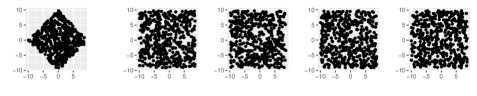
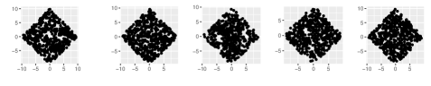
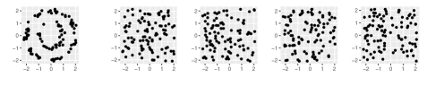
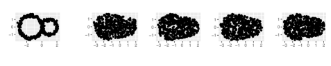
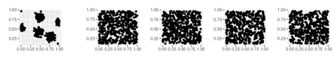
Figure 2. Some examples of point clouds and their axis-aligned or convex hull estimated null model point clouds. The first two rows are the cross-polytope acyclic model, third row is the concentric circles model with outer radius 2, fourth row is the figure 8 model with left radius 1.5 and the last row is a Thomas process with scale 0.05.
The left-most column is the observed acyclic or cyclic model, and the four columns to the right are sample point clouds drawn from the estimated null model (using estimators, from the top, axis, hull, axis, hull, axis

.

4.3.1. Axis-aligned rectangles

For each coordinate $r$ of the data $x=\{x^{1},\dots,x^{n}\}$, estimate lower and upper bounds $(\hat{a}_{r},\hat{b}_{r})$ for a uniform distribution using the formulas

$${\hat{a}}_{r}=\frac{n\min_{j}\{x_{r}^{j}\}-\max_{j}\{x_{r}^{j}\}}{n-1}\qquad{\hat{b}}_{r}=\frac{n\max_{j}\{x_{r}^{j}\}-\min_{j}\{x_{r}^{j}\}}{n-1}$$

To sample, draw uniformly at random each coordinate $x_{r}\sim\text{Uniform}(\hat{a}_{r},\hat{b}_{r})$ to assemble the next observation $x=(x_{1},\dots,x_{d})$.

4.3.2. Convex hull

Compute the convex hull $H(x)$ of the data $x$. Sample by drawing uniformly at random from this convex hull.

4.3.3. Unbiased convex hull

Compute the convex hull $H(x)$ and its set of boundary vertices $V_{\partial}$. Since the centroid of the convex hull is complicated to compute, we approximate it with the centroid $c_{\partial}$ of the boundary vertices of $H(x)$. Compute

$$\hat{H}(x)=\sqrt{\frac{|x|}{|x|-|V_{\partial}|}}(H(x)-c_{\partial})$$

Up to translation, this is an unbiased estimate of the convex hull.

To sample, draw points uniformly at random from $\hat{H}(x)$.

4.4. Topological invariants

There is a wide range of numeric invariants of persistence diagrams in active use in the community. The classically most commonly used is the “length of the longest bar” (which one might call $L_{\infty}$ persistence norm). Also commonly used are $L_{1}$ and $L_{2}$ versions, taking the “mean bar length” or “root mean bar length square”.

In addition to these “additive” invariants, [4] have studied the universality of distributions of invariants deriving from a “multiplicative” or “log-scale” persistence invariant. For a persistence bar $(b,d)$ with birth parameter value $b$ and death parameter value $d$, instead of the $d-b$ used in the additive persistence norms, Bobrowski and Skraba study invariants defined in terms of $\log\log(d/b)$. The result is invariants that measure shape independent of not just translation, but independent also of scaling of point clouds.

[4] define two families of invariants, defined for each persistence bar separately:

• $\pi=d/b$.

• $\ell=\log\log(d/b)-\mu-\gamma$, where $\mu$ is the mean of all the $\log\log(d/b)$ quantities, and $\gamma\approx 0.5772156649$ is the Euler-Mascheroni constant.

These are subsequently summarized across all the persistence bars. We use the $L_{1},L_{2},L_{\infty}$ norms as for the additive invariants to summarize $\pi$ and $\ell$.

We use 21 invariants in our data generation:

For each homological dimension $d=\{0,1,2\}$, and for each of $L_{1},L_{2},L_{\infty}$ we compute the corresponding persistence norm of the Betti $d$ persistence diagram. We denote these as L1.$d$, L2.$d$ and Linf.$d$.

For each homological dimension $d=\{1,2\}$, and each of $L_{1},L_{2},L_{\infty}$, and each of $\pi,\ell$ we compute the corresponding norm of the corresponding bar invariant of the Betti $d$ persistence diagram. We denote these as pi.L$p$.$d$ and ell.L$p$.$d$, where $p\in\{1,2,\infty\}$.

5. Experiments: Questions and results

There are a number of questions we intend to answer by using these pre-computed topological invariants.

• Can these standardized topological invariants really be compared with each other?

• Validate and measure statistical power for the one-sample test described in Method 1.

• Evaluate whether the unbiased convex hull estimator is really needed.

• Validate and measure power for the FWER correction method described in Method 2.

• Validate and measure power for a composite FWER correction method, using several different invariants. A natural approach is to combine all homological dimensions into one composite test.

• Evaluate the differences in performance between the additive and the two multiplicative invariants.

For our validation attempts, we shall in each case study both how close the p-value distribution is to uniform, and what the corresponding empirical levels are for cutoffs chosen to produce $\alpha\in\{0.01,0.05,0.10\}$.

We shall proceed to address each of these questions with corresponding computations now.

5.1. Exchangeability

Can our invariants when computed on point clouds of different sizes and shapes really be compared with each other? We have reasons to believe so – as described in Section 3.2, as well as in the work by Bobrowski and Skraba [4].

For an experimental investigation, we draw 100 acyclic models at random from our full collection of models, estimate and simulate 100 point clouds for each model, and standardize all topological invariants for each of these models. In Figure 3 we show the ECDF for all of these options and all the invariants in one single plot. While there is some variation around a core curve, notice there are no dramatic outliers among all these curves.

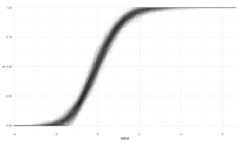
Figure 3. ECDFs of each topological invariant of a sample of 100 standardized simulated point clouds for each of 100 different randomly selected acyclic model setups.

5.2. Bias of the convex hull

Consider the axis-aligned rectangles. We know that estimating these with axis-aligned rectangles is going to give us an unbiased result.

We repeat 100 times drawing an axis-aligned rectangle acyclic model at random from the 16 different versions we have defined. For each acyclic model, we estimate it in three different ways, and for each resulting null model we draw 100 null model point clouds. We compute the p-values, and extract 100 different p-values for each topological invariant and each estimation method.

Since these are p-values from a null-model, we should expect them to be uniformly distributed. In Figure 4, we see the QQ-plots against a uniform distribution split up by estimator and by persistence norm.

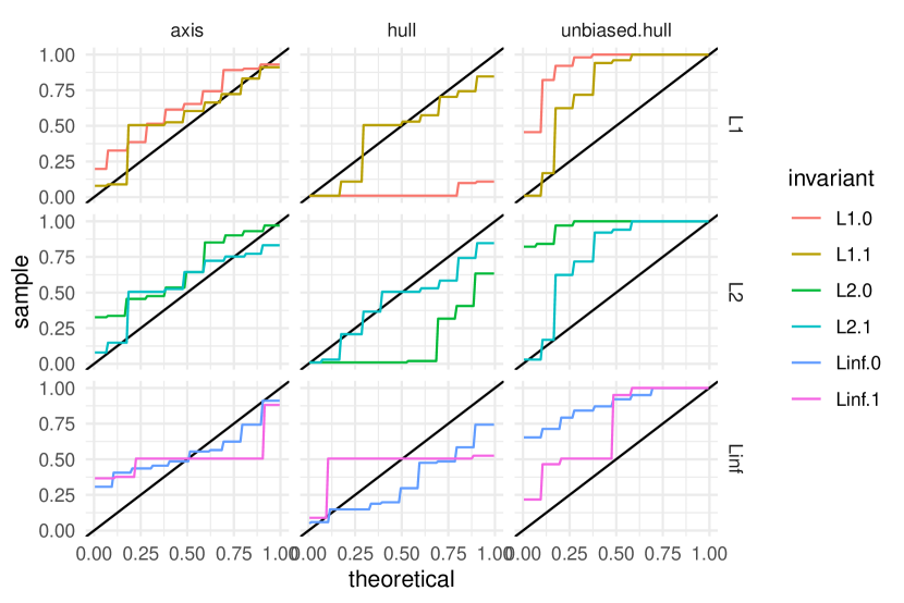
Figure 4. In the left-most column, what we would expect accurate and unbiased estimation and null models to look like. In the middle, the undilated convex hull results. To the right, the results from dilating the convex hull estimation as described. Best results among the convex hull approaches are achieved with the $L_{\infty}$ persistence norm methods and the dilated unbiased convex hull estimation method, while $L_{1}$ and $L_{2}$ perform worse in the unbiased convex hull approach, and all the biased hull methods perform worse again.

The consequences of these discrepancies becomes clear when we look in Table 1 at rejection rates at different intended rejection levels $\alpha$: the rejection rates for the biased convex hull column – especially in homological dimension 0 – look more like power computation numbers than level estimations. The bias is large enough to skew the additive topological invariants enough to give massive amounts of false positives (94% false positives at $\alpha=0.01$ if one were using L1.0).

Invariant	axis	hull	unbiased hull
Linf.0	.08/.15/.28	.21/.29/.38	.02/.05/.05
Linf.1	.03/.07/.10	.02/.10/.22	.03/.03/.05
L1.0	.00/.00/.08	.94/.96/.96	.00/.03/.09
L1.1	.06/.06/.24	.10/.26/.36	.08/.08/.10
L2.0	.05/.09/.13	.82/.88/.92	.00/.00/.06
L2.1	.06/.13/.28	.22/.32/.44	.05/.08/.12

Table 1. Rejection rates by estimator and invariant for an axis-aligned rectangular acyclic model. Rates for $\alpha=0.01/0.05/0.10$ are separated with $/$ in each table cell.

In subsequent experiments we shall ignore the biased convex hull estimator.

5.3. Validate the one-hypothesis one-sample test

For each of the acyclic model types, we repeat 100 times a drawing one acyclic model at random, and then estimate it with the axis and unbiased hull methods and draw 100 null model point clouds. We compute p-values and extract the resulting 100 different p-values for each topological invariant and estimation method.

In Figure 5 we see the QQ-plots for each type of acyclic model we use and each type of additive invariant. Most cases will end up under-producing false positives according to this plot, something can see reflected in Table 5.3.

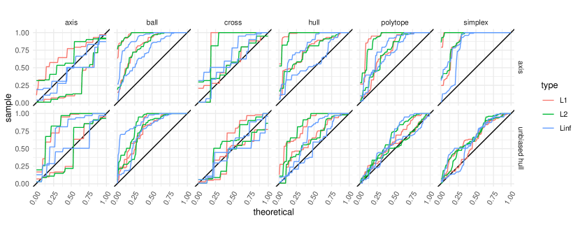
Figure 5. QQ-plot for p-values split up by acyclic model type and by estimator type. The fact that these QQ-curves almost all lie over the diagonal line means that in almost all cases, we under-produce false positives.

Model	Invariant	axis	unbiased hull
axis	L1.0	0.00/0.00/0.00	0.00/0.00/0.00
	L1.1	0.11/0.21/0.55	0.00/0.00/0.19
	L2.0	0.00/0.00/0.00	0.00/0.00/0.00
	L2.1	0.21/0.31/0.42	0.00/0.08/0.15
	Linf.0	0.00/0.00/0.00	0.00/0.00/0.00
	Linf.1	0.00/0.10/0.10	0.00/0.08/0.08
ball	L1.0	0.00/0.00/0.00	0.00/0.02/0.03
	L1.1	0.00/0.00/0.00	0.00/0.00/0.00
	L2.0	0.00/0.00/0.00	0.00/0.01/0.01
	L2.1	0.00/0.00/0.00	0.00/0.00/0.00
	Linf.0	0.00/0.00/0.00	0.00/0.00/0.01
	Linf.1	0.00/0.02/0.02	0.01/0.01/0.01
cross	L1.0	0.18/0.18/0.18	0.13/0.13/0.21
	L1.1	0.00/0.00/0.00	0.00/0.22/0.32
	L2.0	0.18/0.18/0.18	0.13/0.13/0.21
	L2.1	0.00/0.00/0.00	0.00/0.00/0.32
	Linf.0	0.11/0.11/0.19	0.13/0.13/0.23
	Linf.1	0.00/0.00/0.00	0.00/0.00/0.11
random.hull	L1.0	0.00/0.00/0.00	0.00/0.00/0.00
	L1.1	0.00/0.00/0.00	0.10/0.10/0.10
	L2.0	0.00/0.00/0.00	0.00/0.00/0.00
	L2.1	0.00/0.00/0.00	0.10/0.10/0.10
	Linf.0	0.00/0.00/0.02	0.00/0.00/0.09
	Linf.1	0.00/0.02/0.02	0.01/0.04/0.09
random.polytope	L1.0	0.00/0.00/0.00	0.02/0.02/0.07
	L1.1	0.00/0.02/0.07	0.01/0.03/0.04
	L2.0	0.00/0.00/0.00	0.00/0.02/0.07
	L2.1	0.00/0.02/0.04	0.01/0.03/0.08
	Linf.0	0.00/0.05/0.05	0.04/0.04/0.04
	Linf.1	0.00/0.00/0.05	0.00/0.02/0.13
simplex	L1.0	0.00/0.00/0.00	0.01/0.03/0.09
	L1.1	0.00/0.00/0.00	0.00/0.02/0.04
	L2.0	0.00/0.00/0.00	0.02/0.03/0.05
	L2.1	0.00/0.00/0.00	0.00/0.00/0.02
	Linf.0	0.01/0.02/0.02	0.00/0.03/0.11
	Linf.1	0.00/0.00/0.00	0.00/0.02/0.03

Table 2. Rejection rates by acyclic model, estimator and invariant for each type of acyclic model. Rates for $\alpha=0.01/0.05/0.10$ are separated with $/$ in each table cell.

If we look instead at overall rejection rates, without splitting them up at all, we get the results in Table 5.3. These rejection rates are not terribly far off from the intended 0.01/0.05/0.10.

Table 3. Rejection rates across all acyclic models. Rates for $\alpha=0.01/0.05/0.10$ are separated with $/$ in each table cell.

5.4. Power of the one-sample test

We expect the power of the on-sample test to vary with the sample size, the topological shape to be discovered, the null estimator, and the amount of noise in the data. To estimate this power, we sample 100 times with replacement from the 5 iterations of data computed for each combination of noise levels, sample sizes, dimensions, estimators. For each sampled iteration, we compute 100 simulated point clouds and use Method 1 to generate a p-value. This p-value is used against levels of 0.01, 0.05 and 0.10 to generate rejections.

In Table 5.3, we show the power of the one-sample test to detect a topological structure, separated by noise levels, sample sizes, estimators, and invariants used.

We include ECDF-plots for each type of power estimation model in Appendix LABEL:app:power-plots.

Estimator	Invariant	Noise	25	50	100	500
axis	L1	0.01	0.80/0.87/0.97	0.80/0.80/0.80	1.00/1.00/1.00	0.00/0.00/0.00
		0.05	0.20/0.20/0.20	0.20/0.27/0.38	0.00/0.00/0.00	0.00/0.00/0.00
		0.1	0.20/0.35/0.40	0.00/0.12/0.20	0.00/0.00/0.00	0.00/0.00/0.00
	L2	0.01	0.82/0.99/1.00	0.80/0.80/0.80	1.00/1.00/1.00	1.00/1.00/1.00
		0.05	0.20/0.20/0.21	0.60/0.60/0.60	0.41/0.53/0.71	0.80/0.80/0.80
		0.1	0.20/0.35/0.40	0.02/0.19/0.25	0.00/0.00/0.00	0.00/0.00/0.00
	Linf	0.01	0.26/0.60/0.62	0.80/0.80/0.80	1.00/1.00/1.00	1.00/1.00/1.00
		0.05	0.02/0.02/0.02	0.43/0.59/0.60	0.49/0.98/1.00	1.00/1.00/1.00
		0.1	0.40/0.40/0.40	0.00/0.27/0.60	0.00/0.16/0.37	0.40/0.41/0.48
unbiased.hull	L1	0.01	0.62/0.79/0.80	0.60/0.74/0.80	0.83/0.99/1.00	0.00/0.00/0.00
		0.05	0.20/0.20/0.22	0.40/0.46/0.59	0.00/0.05/0.19	0.00/0.00/0.00
		0.1	0.20/0.23/0.35	0.00/0.12/0.20	0.00/0.00/0.00	0.00/0.00/0.00
	L2	0.01	0.80/0.80/0.91	0.80/0.80/0.80	1.00/1.00/1.00	1.00/1.00/1.00
		0.05	0.20/0.20/0.30	0.60/0.60/0.60	0.63/0.78/0.80	1.00/1.00/1.00
		0.1	0.20/0.26/0.38	0.40/0.40/0.40	0.00/0.00/0.10	0.00/0.00/0.00
	Linf	0.01	0.40/0.47/0.58	0.80/0.80/0.80	1.00/1.00/1.00	1.00/1.00/1.00
		0.05	0.20/0.23/0.35	0.60/0.60/0.64	1.00/1.00/1.00	1.00/1.00/1.00
		0.1	0.06/0.21/0.22	0.24/0.52/0.66	0.40/0.56/0.63	0.42/0.60/0.66

Table 4. Rejection rates across all Figure 8 power models, using homological dimension 1. Rates for $\alpha=0.01/0.05/0.10$ are separated with $/$ in each table cell.

5.5. Bobrowski-Skraba multiplicative invariants

The multiplicative invariants $\pi$ and $\ell$ from [4] are designed to be scale-invariant as well as translation-invariant. This reflects in our setting in these invariants handling the unbiased convex hull far better than the additive invariants.

To validate our one-sample hypothesis test with multiplicative invariants, we perform 100 experiments for each acyclic model type; in each experiment we draw one acyclic model at random, and estimate it with all three estimators and draw 100 null model point clouds. We compute p-values and extract the resulting 100 different p-values for each multiplicative invariant and estimation method. The resulting rejection rates at levels of $\alpha=0.01,0.05,0.10$ are reported in Table 5.3.

Table 5. Rejection rates by acyclic model, estimator and invariant for each type of acyclic model using the multiplicative invariants $\pi$ and $\ell$. Rates for $\alpha=0.01/0.05/0.10$ are separated with $/$ in each table cell.

The overall rejection rates (not splitting by acyclic model type) computed by sampling 100 acyclic models from each type, but summarizing the rejection rates without splitting the count on model types are reported in Table 5.3.

Table 6. Rejection rates across all types of acyclic model, for each estimator and invariant using the multiplicative invariants $\pi$ and $\ell$. Rates for $\alpha=0.01/0.05/0.10$ are separated with $/$ in each table cell.

5.6. Validate the FWER control method

To validate the FWER control method, we do the following experiment 100 times:

1. Draw a number $k$ of observed point clouds at random from a Poisson distribution with mean 10.

2. Draw $k$ acyclic models at random from all the models we have defined.

3. For each estimator (axis and unbiased hull) draw 100 null model point clouds for each observed point cloud, and compute standardized topological invariants for each.

4. Maximize invariants, rank and compute p-values.

The resulting p-values are displayed in QQ-plots against a uniform distribution in Figure 6, and corresponding rejection rates for $\alpha=0.01/0.05/0.10$ are reported in Table 5.3.

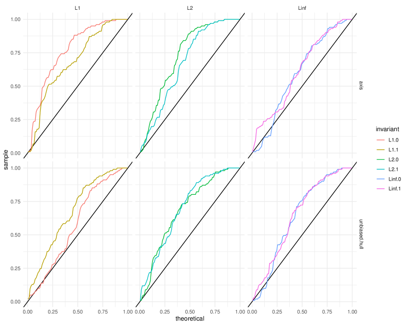
Figure 6. QQ-plots for the FWER procedure on collections of acyclic point clouds against a uniform distribution.

Table 7. Rejection rates for the FWER procedure as applied to randomly selected collections of acyclic point clouds. We have excluded the cross-polytope acyclic models due to their surprisingly high rejection rates already in the single-hypothesis case. Rates for $\alpha=0.01/0.05/0.10$ are separated with $/$ in each table cell.

5.7. Power of the FWER control method

To estimate statistical power the FWER control method, we do the following experiment 100 times for each of the power estimation model types:

1. Draw a number $k$ of observed point clouds at random from a Poisson distribution with mean 10.

2. Draw one power estimation model at random from the given model type.

3. Draw $k-1$ acyclic models at random from all the models we have defined.

4. For each estimator (axis and unbiased hull) draw 100 null model point clouds for each observed point cloud, and compute standardized topological invariants for each.

5. Maximize invariants, rank and compute p-values.

The resulting p-values are displayed in ECDF-plots in Figure 7, and corresponding rejection rates for $\alpha=0.01/0.05/0.10$ are reported in Table 5.3.

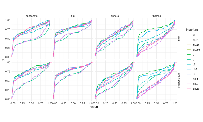
Figure 7. ECDF-plots for the FWER procedure on collections of acyclic point clouds with a single power estimation point cloud, split by type of power estimation.

Table 8. Rejection rates for the FWER procedure as applied to randomly selected collections of acyclic point clouds, with a single power estimation point cloud included. We have excluded the cross-polytope acyclic models due to their surprisingly high rejection rates already in the single-hypothesis case. Rates for $\alpha=0.01/0.05/0.10$ are separated with $/$ in each table cell.

We may of course expect the impact of noise on the detection power to be stark. To this end, in Table 5.3 we give overall rejection rates for the concentric, fig8 and sphere(2) power models in the plane, split up by noise levels. For all of these models, we expect to see a non-trivial $H_{1}$.

For these noise level rejection rates, we repeat the procedure above 100 times for each noise level in $\{0.01,0.05,0.1\}$, but restrict the model types to the planar datasets with the corresponding added noise level.

Table 9. Rejection rates for the FWER procedure as applied to randomly selected collections of acyclic point clouds, with a single planar power estimation point cloud of a specific noise level included. We have excluded the cross-polytope acyclic models due to their surprisingly high rejection rates already in the single-hypothesis case. Rates for $\alpha=0.01/0.05/0.10$ are separated with $/$ in each table cell.

5.8. Using multiple different invariants

Our final experiments are to illustrate the observations in Section 3.5 by showing validation and statistical power for composite invariants. For each of the $L_{1},L_{2},L_{\infty}$ and each three versions of the $\ell$ and $\pi$ invariants, we create a compositve invariant by combining the invariants as evaluated in each homological dimension. We also try combining all the $L_{p}$ invariants in all dimensions into one composite invariant, all the $\pi$ invariants in all dimensions into one, and all the $\ell$ invariants in all dimensions into a final compositve invariant.

In Figure 8 we show the QQ-plots against a uniform distribution for the single-hypothesis case with composite invariants, and in Figure 9, we show QQ-plots for a multiple hypothesis case.

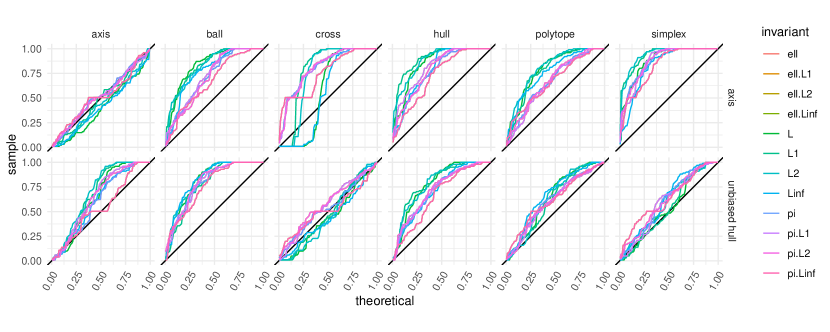
Figure 8. QQ-plots for the single-hypothesis case of all the composite invariants we study here, split up by acyclic model type and null model estimator.

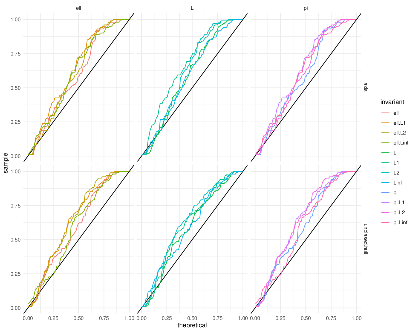
Figure 9. QQ-plots for FWER method for all composite invariants we study here, split up by type ($L_{1}/L_{2}/L_{\infty}$ or $\pi$ or $\ell$) and by null model estimator.

In Table LABEL:tab:reject-rates-acyclic-composite-validation we show rejection rates for the single-hypothesis composite invariant case, and in Table LABEL:tab:reject-rates-acyclic-fwer-composite-validation we show rejection rates for the multiple-hypothesis composite invariant case. For power estimation, we give rejection rates in Table LABEL:tab:reject-rates-power-fwer-composite.

Model	Invariant	axis	unbiased hull
axis	ell	0.02/0.05/0.11	0.04/0.08/0.13
	ell.L1	0.02/0.05/0.09	0.03/0.03/0.10
	ell.L2	0.03/0.04/0.08	0.03/0.09/0.10
	ell.Linf	0.01/0.04/0.06	0.01/0.07/0.07
	L	0.08/0.14/0.21	0.03/0.04/0.16
	L1	0.02/0.08/0.12	0.03/0.03/0.10
	L2	0.05/0.11/0.18	0.01/0.05/0.12
	Linf	0.06/0.13/0.19	0.01/0.06/0.14
	pi	0.02/0.05/0.11	0.04/0.08/0.13
	pi.L1	0.02/0.05/0.09	0.03/0.03/0.10
	pi.L2	0.03/0.04/0.08	0.03/0.09/0.10
	pi.Linf	0.01/0.04/0.06	0.01/0.07/0.07
ball	ell	0.01/0.03/0.04	0.00/0.00/0.03
	ell.L1	0.01/0.01/0.01	0.00/0.00/0.01
	ell.L2	0.01/0.01/0.04	0.00/0.00/0.01
	ell.Linf	0.00/0.03/0.05	0.02/0.02/0.03
	L	0.01/0.03/0.03	0.00/0.01/0.03
	L1	0.01/0.01/0.01	0.01/0.01/0.05
	L2	0.01/0.01/0.03	0.01/0.01/0.02
	Linf	0.00/0.02/0.03	0.00/0.02/0.03
	pi	0.01/0.03/0.04	0.00/0.00/0.03
	pi.L1	0.01/0.01/0.01	0.00/0.00/0.01
	pi.L2	0.01/0.01/0.04	0.00/0.00/0.01
	pi.Linf	0.00/0.03/0.05	0.02/0.02/0.03
cross	ell	0.00/0.00/0.03	0.00/0.03/0.05
	ell.L1	0.00/0.01/0.03	0.02/0.07/0.08
	ell.L2	0.00/0.01/0.01	0.01/0.02/0.04
	ell.Linf	0.00/0.00/0.01	0.00/0.01/0.04
	L	0.26/0.32/0.36	0.12/0.17/0.25
	L1	0.14/0.14/0.15	0.14/0.16/0.18
	L2	0.15/0.16/0.16	0.10/0.15/0.19
	Linf	0.25/0.30/0.35	0.02/0.08/0.16
	pi	0.00/0.00/0.03	0.00/0.03/0.05
	pi.L1	0.00/0.01/0.03	0.02/0.07/0.08
	pi.L2	0.00/0.01/0.01	0.01/0.02/0.04
	pi.Linf	0.00/0.00/0.01	0.00/0.01/0.04
random.hull	ell	0.00/0.00/0.01	0.02/0.04/0.04
	ell.L1	0.00/0.00/0.02	0.02/0.03/0.05
	ell.L2	0.00/0.00/0.01	0.03/0.03/0.05
	ell.Linf	0.00/0.01/0.02	0.01/0.02/0.03
	L	0.00/0.00/0.00	0.01/0.03/0.04
	L1	0.00/0.00/0.00	0.02/0.03/0.04
	L2	0.00/0.00/0.00	0.02/0.03/0.05
	Linf	0.00/0.00/0.01	0.00/0.02/0.03
	pi	0.00/0.00/0.01	0.02/0.04/0.04
	pi.L1	0.00/0.00/0.02	0.02/0.03/0.05
	pi.L2	0.00/0.00/0.01	0.03/0.03/0.05
	pi.Linf	0.00/0.01/0.02	0.01/0.02/0.03
random.polytope	ell	0.00/0.01/0.03	0.00/0.03/0.07
	ell.L1	0.00/0.04/0.06	0.01/0.05/0.08
	ell.L2	0.00/0.02/0.05	0.01/0.04/0.11
	ell.Linf	0.01/0.01/0.03	0.00/0.01/0.04
	L	0.00/0.00/0.02	0.04/0.06/0.09
	L1	0.00/0.02/0.05	0.01/0.05/0.08
	L2	0.00/0.02/0.03	0.00/0.04/0.06
	Linf	0.01/0.02/0.02	0.03/0.06/0.08
	pi	0.00/0.01/0.03	0.00/0.03/0.07
	pi.L1	0.00/0.04/0.06	0.01/0.05/0.08
	pi.L2	0.00/0.02/0.05	0.01/0.04/0.11
	pi.Linf	0.01/0.01/0.03	0.00/0.01/0.04
simplex	ell	0.00/0.00/0.01	0.00/0.02/0.08
	ell.L1	0.00/0.01/0.01	0.00/0.08/0.12
	ell.L2	0.00/0.00/0.01	0.00/0.01/0.05
	ell.Linf	0.00/0.00/0.00	0.00/0.03/0.03
	L	0.00/0.01/0.02	0.05/0.08/0.15
	L1	0.00/0.01/0.01	0.01/0.10/0.14
	L2	0.00/0.00/0.00	0.03/0.05/0.07
	Linf	0.00/0.01/0.01	0.02/0.05/0.07
	pi	0.00/0.00/0.01	0.00/0.02/0.08
	pi.L1	0.00/0.01/0.01	0.00/0.08/0.12
	pi.L2	0.00/0.00/0.01	0.00/0.01/0.05
	pi.Linf	0.00/0.00/0.00	0.00/0.03/0.03

Model	Invariant	axis	unbiased hull
concentric	ell	0.48/0.53/0.60	0.42/0.55/0.57
	ell.L1	0.18/0.29/0.33	0.13/0.22/0.26
	ell.L2	0.44/0.49/0.54	0.43/0.50/0.55
	ell.Linf	0.45/0.51/0.53	0.45/0.51/0.54
	L	0.48/0.55/0.58	0.47/0.61/0.61
	L1	0.17/0.28/0.32	0.13/0.22/0.26
	L2	0.44/0.50/0.54	0.42/0.49/0.55
	Linf	0.46/0.50/0.54	0.49/0.59/0.61
	pi	0.48/0.53/0.60	0.42/0.55/0.57
	pi.L1	0.18/0.29/0.33	0.13/0.22/0.26
	pi.L2	0.44/0.49/0.54	0.43/0.50/0.55
	pi.Linf	0.45/0.51/0.53	0.45/0.51/0.54
fig8	ell	0.63/0.66/0.68	0.63/0.65/0.69
	ell.L1	0.36/0.42/0.44	0.35/0.41/0.45
	ell.L2	0.54/0.60/0.65	0.57/0.64/0.66
	ell.Linf	0.57/0.59/0.62	0.55/0.61/0.68
	L	0.60/0.65/0.67	0.62/0.66/0.68
	L1	0.36/0.41/0.43	0.34/0.40/0.45
	L2	0.53/0.59/0.64	0.57/0.62/0.65
	Linf	0.54/0.58/0.62	0.53/0.61/0.63
	pi	0.63/0.66/0.68	0.63/0.65/0.69
	pi.L1	0.36/0.42/0.44	0.35/0.41/0.45
	pi.L2	0.54/0.60/0.65	0.57/0.64/0.66
	pi.Linf	0.57/0.59/0.62	0.55/0.61/0.68
sphere	ell	0.26/0.32/0.35	0.26/0.28/0.31
	ell.L1	0.13/0.14/0.19	0.08/0.11/0.15
	ell.L2	0.21/0.24/0.30	0.23/0.25/0.29
	ell.Linf	0.25/0.32/0.36	0.21/0.25/0.37
	L	0.24/0.32/0.38	0.30/0.39/0.40
	L1	0.12/0.14/0.18	0.08/0.11/0.16
	L2	0.20/0.25/0.29	0.23/0.25/0.30
	Linf	0.23/0.31/0.40	0.27/0.35/0.39
	pi	0.26/0.32/0.35	0.26/0.28/0.31
	pi.L1	0.13/0.14/0.19	0.08/0.11/0.15
	pi.L2	0.21/0.24/0.30	0.23/0.25/0.29
	pi.Linf	0.25/0.32/0.36	0.21/0.25/0.37
thomas	ell	0.10/0.17/0.20	0.10/0.16/0.18
	ell.L1	0.04/0.08/0.16	0.04/0.08/0.11
	ell.L2	0.07/0.10/0.13	0.09/0.11/0.11
	ell.Linf	0.12/0.16/0.20	0.13/0.17/0.21
	L	0.56/0.63/0.67	0.60/0.64/0.66
	L1	0.22/0.24/0.30	0.21/0.27/0.32
	L2	0.34/0.40/0.42	0.36/0.38/0.42
	Linf	0.47/0.53/0.55	0.53/0.59/0.62
	pi	0.10/0.17/0.20	0.10/0.16/0.18
	pi.L1	0.04/0.08/0.16	0.04/0.08/0.11
	pi.L2	0.07/0.10/0.13	0.09/0.11/0.11
	pi.Linf	0.12/0.16/0.20	0.13/0.17/0.21

6. Conclusion

We have proposed testing procedures for coherence with a null model to test for acyclicity (trivial homology), both in a single-hypothesis setting and with control for Family-Wise Error Rate and for False Discovery Rate in both multiple one-sample and multiple two-sample hypothesis test settings. For all of these, we perform both validation tests (measuring rejection rates on acyclic point clouds) and estimate statistical power (measuring rejection rates on point clouds with known topological structure).

The FDR control methods produce the intended rejection rates by construction, if it is possible with the data at hand.

For FWER control methods, we have empirical validation and power measurement in Section 5.

In our computations, we can see low rejection rates for acyclic point clouds (except for the cross-polytope point clouds, for reasons that are not entirely clear to us), and higher rejection rates for point clouds with structure – with the statistical power falling as noise levels rise.

6.1. Limitations

The null model estimation techniques all have significant limitations: the axis-aligned estimation may be a bad fit for the shape of the support, as seen in the cross-polytope case, the biased convex hull method provides a null model on slightly erroneous wcale and both convex hull methods fail completely on data that is contained in a proper affine subspace.

6.2. Recommendations

Based on our experiments, in order to determine acyclicity for either a single point cloud or for a whole collection of related point clouds, we recommend:

• Use a dimension-agnostic invariant – ie, a composite invariant that uses all the homological dimensions available.

• If you care about scale, use the Linf composite invariant. If you don’t care about scale – and you are not seeking information about clustering structures, use the maximum value of the $\pi$ invariants (the pi.Linf composite invariant).

• If your data is contained in a linear subspace of positive co-dimension, use the axis null model estimator, otherwise use the unbiased convex hull estimator.

6.3. Future work

Our simulation experiments do raise some questions. It would be interesting to find out why the rejection rates are so dramatically much higher for the cross-polytope acyclic models than for all the other acyclic models. It would be interesting to see the performance of these methods on concrete problems motivated by real data.

Appendix A Deriving the bounds for a bounding box

To derive the bounds of a bounding box for a uniform distribution on an axis-aligned box, we may treat each axis independently. This reduces the problem to estimating the support $(a,b)$ of a uniform distribution $U(a,b)$. A complete sufficient statistic for this distribution is $T(X)=(X_{(1)},X_{(n)})=(\min_{x\in X}x,\max_{x\in X}x)$. If $X\sim U(a,b)$, then $Y=(X-a)/(b-a)\sim U(0,1)$ and the order statistics of the standard uniform distribution $U(0,1)$ are known to be $Y_{(k)}\sim\mathrm{Beta}(k,n+1-k)$. Hence $Y_{(1)}\sim\mathrm{Beta}(1,n)$, $Y_{(n)}\sim\mathrm{Beta}(n,1)$ and $\mathbb{E}[Y_{(1)}]=1/(n+1)$, $\mathbb{E}[Y_{(n)}]=n/(n+1)$. It follows that

$$\mathbb{E}[X_{(1)}]=\frac{b-a}{n+1}+a\qquad\mathbb{E}[X_{(n)}]=\frac{n(b-a)}{n+1}+a$$

Solving this pair of equations for $a$ and $b$, we get:

$$\hat{a}=\frac{n\mathbb{E}[X_{(1)}]-\mathbb{E}[X_{(n)}]}{n-1}\qquad\hat{b}=\frac{n\mathbb{E}[X_{(n)}]-\mathbb{E}[X_{(1)}]}{n-1}$$

Appendix B Power-analysis plots

Appendix C Example point clouds for the alternative models

ßin 0.01,0.05,0.1

in 1.25,2,5,10 $r=\rr$  in 25,50,100,500

ßin 0.01,0.05,0.1

in 0.25,0.5,1,1.5,5 $r=\rr$  in 25,50,100,500

ßin 0.05,0.1,0.15,0.2,0.25 $\sigma^{2}=\ss$

in 25,50,100,500

Appendix D Rejection rates for all our models

For each model specification, we create a bootstrap estimate by repeating 20 times the drawing one of the 5 realizations of that model specification at random, and then draw 100 estimated null model point clouds for each estimation method to compute a p-value for that realizations. The resulting rates are in the supplemental file reject-rates-individual-fods.csv, and the simulated p-values in the supplemental file p-values-individual-fods.csv.

References

- [1] Adrian Baddeley and Rolf Turner. spatstat: An R package for analyzing spatial point patterns. Journal of Statistical Software, 12(6):1–42, 2005. doi:10.18637/jss.v012.i06.
- [2] Ulrich Bauer. Ripser: efficient computation of vietoris-rips persistence barcodes. Journal of Applied and Computational Topology, 2021. doi:10.1007/s41468-021-00071-5.
- [3] Andrew J. Blumberg, Itamar Gal, Michael A. Mandell, and Matthew Pancia. Robust statistics, hypothesis testing, and confidence intervals for persistent homology on metric measure spaces. Foundations of Computational Mathematics, 14(4):745–789, 2014. URL: http://link.springer.com/article/10.1007/s10208-014-9201-4.
- [4] Omer Bobrowski and Primoz Skraba. On the universality of random persistence diagrams, 2022. URL: https://arxiv.org/abs/2207.03926, doi:10.48550/ARXIV.2207.03926.
- [5] Carlo Bonferroni. Sulle medie multiple di potenze. Bollettino dell’Unione Matematica Italiana, 5(3-4):267–270, 1950.
- [6] Peter Bubenik. Statistical topological data analysis using persistence landscapes. The Journal of Machine Learning Research, 16(1):77–102, 2015. URL: http://arxiv.org/abs/1207.6437.
- [7] Christopher Cericola, Inga Johnson, Joshua Kiers, Mitchell Krock, Jordan Purdy, and Johanna Torrence. Extending Hypothesis Testing with Persistence Homology to Three or More Groups. Involve, a Journal of Mathematics, 11(1):27–51, January 2018. arXiv: 1602.03760. URL: http://arxiv.org/abs/1602.03760, doi:10.2140/involve.2018.11.27.
- [8] Frédéric Chazal, Brittany Fasy, Fabrizio Lecci, Bertrand Michel, Alessandro Rinaldo, Alessandro Rinaldo, and Larry Wasserman. Robust topological inference: Distance to a measure and kernel distance. The Journal of Machine Learning Research, 18(1):5845–5884, 2017. URL: http://arxiv.org/abs/1412.7197.
- [9] Frédéric Chazal, Brittany Fasy, Fabrizio Lecci, Bertrand Michel, Alessandro Rinaldo, and Larry Wasserman. Subsampling methods for persistent homology. In International Conference on Machine Learning, pages 2143–2151, 2015. URL: http://arxiv.org/abs/1406.1901.
- [10] Frédéric Chazal, Brittany Terese Fasy, Fabrizio Lecci, Alessandro Rinaldo, Aarti Singh, and Larry Wasserman. On the Bootstrap for Persistence Diagrams and Landscapes. arXiv:1311.0376 [cs, math, stat], November 2013. URL: http://arxiv.org/abs/1311.0376.
- [11] Microsoft Corporation and Steve Weston. doParallel: Foreach Parallel Adaptor for the ’parallel’ Package, 2022. R package version 1.0.17. URL: https://CRAN.R-project.org/package=doParallel.
- [12] Brittany Terese Fasy, A. Rinaldo, and L. Wasserman. Stochastic Convergence of Persistence Landscapes and Silhouettes. Convergence, (1/25), 2014.
- [13] Vissarion Fisikopoulos, Apostolos Chalkis, and contributors in file inst/AUTHORS. volesti: Volume Approximation and Sampling of Convex Polytopes, 2021. R package version 1.1.2-2. URL: https://CRAN.R-project.org/package=volesti.
- [14] Alan Genz, Frank Bretz, Tetsuhisa Miwa, Xuefei Mi, Friedrich Leisch, Fabian Scheipl, and Torsten Hothorn. mvtnorm: Multivariate Normal and t Distributions, 2021. R package version 1.1-3. URL: https://CRAN.R-project.org/package=mvtnorm.
- [15] Kai Habel, Raoul Grasman, Robert B. Gramacy, Pavlo Mozharovskyi, and David C. Sterratt. geometry: Mesh Generation and Surface Tessellation, 2022. R package version 0.4.6.1. URL: https://CRAN.R-project.org/package=geometry.
- [16] A. Hatcher. Algebraic topology. Cambridge University Press, 2002.
- [17] Yasuaki Hiraoka, Tomoyuki Shirai, and Khanh Duy Trinh. Limit theorems for persistence diagrams. The Annals of Applied Probability, 28(5):2740–2780, October 2018. doi:10.1214/17-AAP1371.
- [18] Yosef Hochberg. A sharper bonferroni procedure for multiple tests of significance. Biometrika, 75(4):800–802, 1988. URL: http://dx.doi.org/10.1093/biomet/75.4.800, arXiv:/oup/backfile/content_public/journal/biomet/75/4/10.1093/biomet/75.4.800/2/75-4-800.pdf, doi:10.1093/biomet/75.4.800.
- [19] Sture Holm. A simple sequentially rejective multiple test procedure. Scandinavian journal of statistics, pages 65–70, 1979.
- [20] K. Korthauer, P.K. Kimes, C. Duvallet, A. Reyes, A. Subramanian, M. Teng, C. Shukla, E.J. Alm, and S.C. Hicks. A practical guide to methods controlling false discoveries in computational biology. Genome Biology, 20(118), 2019.
- [21] EH Lloyd. Least squares estimation of location and scale parameter using order statistics. Biometrika, (39):88–95, 1952.
- [22] Microsoft and Steve Weston. foreach: Provides Foreach Looping Construct, 2022. R package version 1.5.2. URL: https://CRAN.R-project.org/package=foreach.
- [23] Yuriy Mileyko, Sayan Mukherjee, and John Harer. Probability measures on the space of persistence diagrams. Inverse Problems, 27(12):124007, 2011. URL: http://stacks.iop.org/0266-5611/27/i=12/a=124007.
- [24] Marc Moore. On the estimation of a convex set. The Annals of Statistics, 12(3):1090–10999, 1984.
- [25] Elizabeth Munch, Katharine Turner, Paul Bendich, Sayan Mukherjee, Jonathan Mattingly, and John Harer. Probabilistic Fréchet means for time varying persistence diagrams. Electronic Journal of Statistics, 9(1):1173–1204, 2015.
- [26] T. Nichols and S. Hayasaka. Controlling the familywise error rate in functional neuroimaging: a comparative review. Stat Methods Med Res., 12(5):419–46, 2003.
- [27] Belinda Phipson and Gordon K Smyth. Permutation p-values should never be zero: calculating exact p-values when permutations are randomly drawn. Statistical applications in genetics and molecular biology, 9(1), 2010.
- [28] R Core Team. R: A Language and Environment for Statistical Computing. R Foundation for Statistical Computing, Vienna, Austria, 2022. URL: https://www.R-project.org/.
- [29] JP Rasson. Estimation de formes convexes du plan. Statistiques et Analyse des données, (1):31–46, 1979.
- [30] BD Ripley and JP Rasson. Finding the edge of a poisson forest. Journal of Applied Probability, (14):483–491, 1977.
- [31] Andrew Robinson and Katharine Turner. Hypothesis testing for topological data analysis. Journal of Applied and Computational Topology, November 2017. URL: http://link.springer.com/10.1007/s41468-017-0008-7, doi:10.1007/s41468-017-0008-7.
- [32] Katharine Turner. Means and medians of sets of persistence diagrams. arXiv e-print 1307.8300, July 2013. URL: http://arxiv.org/abs/1307.8300.
- [33] Katharine Turner, Yuriy Mileyko, Sayan Mukherjee, and John Harer. Fréchet means for distributions of persistence diagrams. Discrete & Computational Geometry, 52(1):44–70, 2014.
- [34] Katharine Turner, Sayan Mukherjee, and Doug M. Boyer. Sufficient statistics for shapes and surfaces. Annals of statistics, 2013.
- [35] Mikael Vejdemo-Johansson and Alisa Leshchenko. Certified mapper: Repeated testing for acyclicity and obstructions to the nerve lemma. In Topological Data Analysis, volume 15 of Abel Symposia, pages 491–515. Springer, 2020.
- [36] Raoul Wadhwa, Matt Piekenbrock, Jacob Scott, Jason Cory Brunson, and Xinyi Zhang. ripserr: Calculate Persistent Homology with Ripser-Based Engines, 2022. R package version 0.2.0. URL: https://rrrlw.github.io/ripserr/.
- [37] Hadley Wickham, Mara Averick, Jennifer Bryan, Winston Chang, Lucy D’Agostino McGowan, Romain François, Garrett Grolemund, Alex Hayes, Lionel Henry, Jim Hester, Max Kuhn, Thomas Lin Pedersen, Evan Miller, Stephan Milton Bache, Kirill Müller, Jeroen Ooms, David Robinson, Dana Paige Seidel, Vitalie Spinu, Kohske Takahashi, Davis Vaughan, Claus Wilke, Kara Woo, and Hiroaki Yutani. Welcome to the tidyverse. Journal of Open Source Software, 4(43):1686, 2019. doi:10.21105/joss.01686.