Abstract

Models incorporating moderately heavy dark matter (DM) typically need charged (scalar) fields to establish admissible relic densities. Since the DM freezes out at an early epoch, thermal corrections to the cross sections can be important. In a companion paper [1] we established that the infrared (IR) divergences accruing from scalar-photon interactions cancel to all orders in perturbation theory. The corresponding infrared finiteness of thermal fermionic QED has already been established. Here, we study the IR behaviour at finite temperatures, of a theory of dark matter interacting with charged scalars and fermions, which potentially contains both both linear and sub-leading logarithmic divergences. We prove that the theory is IR-finite to all orders with the divergences cancelling when both absorption and emission of photons from and into the heat bath are taken into account. While 4-point interaction terms are known to be IR finite, their inclusion leads to a neat exponentiation. The calculation follows closely the technique used for the scalar finite temperature theory.

PACs: 11.10.−z, 11.10.Wx, 11.15.−q, 11.30.Pb, 12.60.−i, 95.35.+d

1 Introduction

Astrophysical and cosmological observations spanning over a multitude of length scales, beginning with rotation curves, lensing, on to galactic and cluster collisions, and finally the origin of large scale structure in the Universe as also the power spectrum of the cosmic microwave background radiation, all point to the existence of a mysterious Dark Matter (DM) that overwhelms ordinary matter in the Universe. And while all the evidence so far has come from the study of gravitational effects, simple modifications in the theory of gravity have, so far, failed to account for all the observations. The conundrum, apparently, can be resolved only by postulating a particulate DM that, of necessity, must be immune to strong interactions and, preferably, neutral.

If we posit that the DM particle has no interactions at all with the Standard Model (SM) particles, other than the gravitational, there would be virtually no hope of ever observing it directly in a controlled experiment. Consequently, it is assumed that the DM must have sufficient interactions with at least some of the SM particles, presumably with a strength comparable to weak interactions, or at worst, a couple of order of magnitudes weaker. Such an assumption has a further ramification. A standard assumption in explaining the evolution of the Universe is that all particles—whether those within the SM, or the DM—were created during the (post-inflation) reheating phase. The subsequent number densities are supposed to have been determined by the expansion of the Lemaitre-Friedmann-Robertson-Walker Universe, augmented by a set of coupled Boltzmann equations that are operative when the particles are in equilibrium. If the DM particle $\chi$ does have such interactions, then it can stay in equilibrium with the SM sector via interactions of the form,

$$\chi+\overline{\chi}\leftrightarrow{\cal F}_{SM}+\overline{\cal F}_{SM}\ ,\qquad{\rm and}\qquad\chi+{\cal F}_{SM}\leftrightarrow\chi+{\cal F}_{SM}\ ,$$ (1)

where ${\cal F}_{SM}$ is a particle corresponding to some arbitrary SM field. This equilibrium phase would last until the interaction rate falls below the Hubble expansion rate. With the Universe cooling as it expands, the DM must fall out of equilibrium by the time its mass exceeds the temperature. With large scale structure formation liable to be destroyed in the presence of a dominantly hot DM (i.e., one where the DM decoupled well before the temperature fell down to $m_{\chi}$), the favourite scenario is that of a dominantly cold DM (i.e., one which had become nonrelativistic at the decoupling era). Interestingly, if the interactions governing Eq. 1 typically have a strength comparable to the weak interaction, then for a wide range of masses, ${\cal O}(10)\hbox{ GeV}<m_{\chi}<{\cal O}(10^{4})$ GeV, the relic density is of the required order.

Given the high precision to which the DM contribution to the energy budget has been measured by the wmap [2] and, subsequently, the planck [3] collaborations, an order of magnitude estimation is no longer acceptable, and precise predictions need to be made. Indeed, the measurements have imposed rather severe constraints on several well-motivated models for the DM, to the extent of ostensibly even ruling out some of them. Such drastic conclusions, though, need to be treated with caution, for many of the theoretical estimates have resulted from lowest-order calculations alone. More importantly, the effect of non-zero temperatures are rarely considered. Together, these effects can alter the predictions to a significant degree.

Initial efforts to include thermal corrections to the relevant processes were made in Ref. [4], wherein it was shown, albeit to only the next-to-leading order (NLO), that infra-red divergences (both soft and collinear) cancel out in processes involving both charged scalars and charged fermions. However, no proof to all orders exists so far and we provide one in this paper. In an earlier paper [1], referred to henceforth as Paper I, we had discussed, in detail, the infra red (IR) behaviour, via factorisation and resummation, of theories associated with charged scalar particles, at both zero and finite temperature. In doing this, we proved the IR finiteness of such theories to all orders of perturbation theory. The IR finiteness of thermal fermionic QED has already been established to all orders [10]. In this second paper, we apply the results for thermal fermionic and scalar theories to set out the analogous proof of the IR finiteness of theories associated with bino-like dark matter (DM) models, at non-zero temperatures. While IR finiteness is important to establish the consistency of the theory, the inclusion of such corrections is also crucial for an accurate calculation of the relic density of the DM.

Although it might seem that a bino-like DM candidate is a very specific choice, it actually captures the essence of a wide class of models. Whereas the MSSM spectrum would include, apart from the SM particles, the entire gamut of their supersymmetric partners, only a handful of them play a significant role in determining the relic density. Apart from the DM candidate itself, these are some charged scalars (typically, close to the DM in mass), and occasionally, depending on the details of the supersymmetry breaking scheme, others as well. And while the DM itself is a linear combination of the bino, the neutral wino and the two neutral higgsinos, for a very large class of supersymmetry breaking scenarios, the higgsino mass parameter $\mu$ is much larger than the soft terms ($M_{1,2}$) for the gauginos, thereby suppressing the higgsino component to negligible levels. And since wino-bino mixing is pivoted by $\mu$, a large value for the latter also suppresses the wino-component in the DM. The assumption of a bino-like DM further simplifies the calculations as we may safely neglect additional diagrams, e.g., with $s$-channel gauge bosons or Higgs. It should also be appreciated that no new infrared divergence structures would appear even on the inclusion of such additional mediators. In other words, restricting ourselves to the particular case of the bino does not represent the neglect of subtle issues while allowing for considerable simplifications, both algebraic and in bookkeeping.

The Lagrangian density relevant to this simplified scenario is given by an extension of the Standard Model containing left handed fermion doublets, ${f}=({f}^{0},{f}^{-})^{T}$, with an additional scalar doublet, $\phi=(\phi^{+},\phi^{0})^{T}$, namely the supersymmetric partners of $f$, along with the $SU(2)\times U(1)$ singlet Majorana fermion $\chi$ which is the dark matter candidate. We have,

$${\cal{L}}= -\frac{1}{4}F_{\mu\nu}F^{\mu\nu}+\overline{{f}}\left(i\not{D}-m_{f}\right){{f}}+\frac{1}{2}\overline{\chi}\left(i\not{D}-m_{\chi}\right)\chi$$

$$+\left(D^{\mu}\phi\right)^{\dagger}\left(D_{\mu}\phi\right)-m_{\phi}^{2}\phi^{\dagger}\phi+\left(\lambda\,\overline{\chi}P_{L}{{f}}^{-}\phi^{+}+{\rm h.c.}\right)~{}.$$ (2)

We assume that the bino is a TeV scale DM particle so that freeze-out occurs after the electro-weak transition; hence, only electromagnetic interactions are relevant for the IR finiteness at these scales. In other words, the $\chi$ interacts only with fermions and sfermions, ${{f}}$ and $\phi$, and not with the photon. Thus, only the charged (s)fermion interactions with $\chi$ are shown in Eq. 2 since it is the resummation of the radiative photon diagrams which are of interest here.

The simplest process for DM annihilation (or, equivalently, DM scattering off a SM particle), as driven by the Lagrangian of Eq. 2, is illustrated in Fig. 1. Higher order electromagnetic corrections to such diagrams involve, apart from real photon emissions from either $f$ or $\phi$, virtual photon exchanges as well.

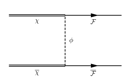
Figure 1: A typical dark matter annihilation/scattering process.

Such contributions can be calculated in a real time formulation of the thermal field theory [5]. In Ref. [6], the eikonal approximation was used and the interaction of photons with a semi-classical current was analysed within the framework of thermal field theory. In Ref. [7], 1-loop corrections to thermal QED were computed for both fermions and scalars. It was found that the finite temperature mass shift for scalar QED when the temperature is less than the scalar mass ($0<T\ll m_{s}$) is identical to the corresponding fermion case as is the IR divergent piece of the wave function and vertex renormalisation constants. However, the contribution to the plasma screening mass was twice that for the fermion loop due to the difference in the form of the thermal distributions (boson versus fermion). In Ref. [8], dynamical renormalisation group resummation of finite temperature IR divergences to 1-loop was done to study relaxation as well as out-of-equilibrium damping in real time for a scalar thermal field theory. This was applied to study IR divergences in scalar QED (to the lowest order in the hard-thermal loop (HTL) resummation). It was found that the infrared divergences in this theory are similar to those found in QED and in lowest order in QCD. Results in thermal scalar QED have also been applied to study Schwinger pair-production [9].

Here we use a similar approach to address the issue of IR finiteness of the thermal field theory of dark matter, thereby combining and extending the results of the earlier work on thermal fermions [10] with the finite temperature results for charged scalars as discussed in Paper I [1].

In Section 2, we set up the real-time formulation of the thermal field theory corresponding to the Lagrangian of Eq. 2 and write down the propagators and vertex factors of the theory. In Section 3, we set up the machinery to address the infrared (IR) finiteness of such a theory of dark matter interacting with charged fermions and scalars. In particular, we take the example of the process $\chi{\cal{F}}\to\chi{\cal{F}}$ where the bino $\chi$ interacts with fermions ${\cal{F}}$ via a bino-fermion-scalar interaction, and all higher order contributions to this process. We outline in Section 3.1 the approach of Grammer and Yennie [11] (henceforth referred to as GY) which was used to address the IR finiteness of fermionic QED at zero temperature through a detailed consideration of the process ${\cal{F}}(p)\gamma^{*}(q)\to{\cal{F}}(p^{\prime})$, which we use in our calculations, by defining the so-called $K$ and $G$ photon insertions and the vertex $V$ that enables use of this approach (Section 3.2). In Section 3.3, we show that the $K$ photon insertions contain the IR divergence and compute these contributions for all possible insertions of the virtual $K$ photons. This section contains the main new results of this paper. Since the calculation heavily depends on the results obtained in earlier work [1, 10], an overview of these results is also presented here.

That the $G$ photon insertions are IR finite is shown in Section 3.4; this result straightforwardly follows from the calculations done earlier [1, 10] and only highlights are included. Emission and absorption of real photons from the heat bath constitude the other set of corrections to the lowest order process of interest. Since the real photon contribution is a straightforward extension of earlier results [1, 10], we simply outline the procedure, and the main complications that arise before writing down the results in Section 3.5.

In Refs. [6, 10, 12] it was shown that pure fermionic thermal QED has both a linear divergence and a logarithmic subdivergence in the infra red compared to the purely logarithmic divergence encountered in the zero temperature theory, owing to the nature of the thermal photon propagator. The same was true for the case of thermal scalar QED as shown in Ref. [1] and is true here as well. We factorise and exponentiate the divergences and show that they cancel order by order between virtual and real photon contributions (the latter include both emission and absorption terms) and hence prove the IR finiteness of a thermal theory of dark matter to all orders. We write down the total cross section to all orders in Section 3.6 where we explicitly demonstrate the IR finiteness of the cross section in the soft limit. Section 4 contains the discussions and conclusions. The appendices are used to set up the Feynman rules (Appendix A) for thermal field theories and to list some useful identities (Appendix B) that are used to factorise the $K$ photon contributions.

2 Real-time formulation of the thermal field theory with dark matter

We briefly review the real-time formulation [5] of thermal (scalar, fermion and photon) fields in equilibrium with a heat bath at temperature $T$. The field theory of such a system is then a statistical field theory with a thermal vacuum defined such that the ensemble average of an operator can be written [13] as its expectation value of time-ordered products in the thermal vacuum. In order to satisfy this requirement, a special path is chosen for the integration in the complex time plane; see Appendix A for details. This results in the fields satisfying the periodic boundary conditions,

$$\varphi(t_{0})=\pm\varphi(t_{0}-i\beta)~{},$$

where $\pm 1$ correspond to boson and fermion fields respectively.

There are two parts of the time path, $C_{1}$ and $C_{2}$, along the real time axis and parallel to it (see details and figure in Appendix A); this gives rise to fields that “live” on the $C_{1}$ or $C_{2}$ line and hence leads to the well-known field-doubling, so that fields are of type-1 (physical) or type-2 (ghosts), with propagators acquiring a $2\times 2$ matrix form. Only type-1 fields can occur on external legs while fields of both types can occur on internal legs, with the off-diagonal elements of the propagator allowing for conversion of one type into another. The zero temperature part of the propagator corresponds to the exchange of a virtual particle, as usual, but the finite temperature part of the propagator represents an on-shell contribution which measures the probability of emitting or absorbing real particles from the medium. See Appendix A for detailed definitions of the scalar, fermion and photon field propagators. Finally, the vertices, both 3-point and 4-point ones, are modified in the thermal theory by extending the Lagrangian given in Eq. 2 to include both kinds of vertices [14]. Details are again in Appendix A; we only note here that all the fields at a given vertex must be of the same thermal type.

In particular, the photon propagator corresponding to a momentum $k$ can be expressed (in the Feynman gauge) as,

$$i{\cal D}^{ab}_{\mu\nu}(k) =-g_{\mu\nu}\,iD^{ab}(k)~{},$$ (3)

where the information on the field type is contained in $D^{ab}(k)$; see Appendix A for its definition. Note that the factor $g_{\mu\nu}$ occurs in all components of the thermal photon propagator, with the relevant part of the thermal photon propagator being

$$i{\cal{D}}^{ab}(k)\sim \left[\frac{i}{k^{2}+i\epsilon}\delta^{ab}\pm 2\pi\,\delta(k^{2})\,N(|{k^{0}}|)\,D^{ab}_{T}\right]~{},$$ (4)

where the first term corresponds to the $T=0$ contribution and the second to the finite temperature part. While the fermionic number operator, viz.,

$$N_{f}(|{p^{0}}|)\equiv\frac{1}{\exp\{|p^{0}|/T\}+1}\;\stackrel{{\scriptstyle p\to 0}}{{\longrightarrow}}\;\frac{1}{2}~{},$$ (5)

is well-defined in the soft limit, the bosonic number operator in the photon propagator contributes an additional power of ${k^{0}}$ in the denominator in the soft limit, since

$$N(|k^{0}|)\equiv\frac{1}{\exp\{|k^{0}|/T\}-1}\;\stackrel{{\scriptstyle k\to 0}}{{\longrightarrow}}\;\frac{T}{|k^{0}|}~{}.$$ (6)

Hence, it can be seen that the leading IR divergence in the finite temperature part is linear rather than logarithmic as was the case at zero temperature. Consequently, there is a residual logarithmic subdivergence that must also be shown to cancel at finite temperatures, thus making the generalisation to the thermal case non-trivial.

It was shown in two earlier papers [1, 10] that thermal field theories of pure scalar and spinor electrodynamics are IR finite to all orders in the theory. The object of this paper is to obtain an analogous proof of IR finiteness for a thermal field theory of (charge-neutral) dark matter interacting with both charged scalars and charged fermions with these additional complications.

3 The IR finiteness of the thermal field theory with dark matter

The companion paper, Paper I, established that a field theory of charged scalars is IR finite to all orders both at $T=0$ and at finite temperature. The corresponding all-order proof for fermionic QED is already known [10]. We now apply and extend these two results to prove the IR finiteness to all orders of theories of dark matter at finite temperature. The proof involves obtaining a neat factorisation and exponentiation of the soft terms to all orders in the theory, with order by order cancellation between the IR divergent contributions of virtual and real photon corrections to the leading order contribution.

3.1 The Grammer Yennie approach

We use the approach of Grammer and Yennie [11], as applied in the earlier papers as well. We briefly outline their approach, which was used to prove the IR finiteness of zero temperature fermionic QED. Their proof technique involved starting at an $n^{\rm th}$ order correction (with real or virtual photons) to the process $e(p)\gamma^{*}(q)\to e(p^{\prime})$ (where $q$ is a hard momentum flowing in at the vertex $V$, and the remaining $n$ photon momenta can be arbitrarily soft), and examining the effect of adding an additional virtual or real $(n+1)^{\rm th}$ photon with momentum $k$ to this graph, in all possible ways.

In particular, in order to separate out the IR divergent piece in a virtual photon insertion, the corresponding photon propagator of the newly inserted photon was written as the sum over so-called $K$- and $G$-photon contributions, viz.,

$$-i\frac{g_{\mu{\nu}}}{k^{2}+i\epsilon} =\frac{-i}{k^{2}+i\epsilon}\,\left\{\left[g_{\mu\nu}-b_{k}(p_{f},p_{i})\,k_{\mu}k_{\nu}\right]+\left[b_{k}(p_{f},p_{i})k_{\mu}k_{\nu}\right]\right\}~{},$$

$$\equiv\frac{-i}{k^{2}+i\epsilon}\,\left\{\left[G\right]+\left[K\right]\right\}~{},$$ (7)

where $b_{k}$ (to be defined later below) is a function of $k$ as well as the momenta, $p_{f}$, $p_{i}$, of the final and initial particles, i.e., just after (before) the final (initial) vertex, and is defined so that all the IR divergences are collected into the $K$-photon contributions. The key to this factorisation lies in recognising that the insertion of a virtual $K$ photon vertex $\mu$ on a fermion line is equivalent to the insertion $\gamma^{\mu}k_{\mu}\equiv/{\!\!\!k}$ at the vertex $\mu$. The contribution due to the insertion can be expressed, courtesy generalised Feynman identities (see Eq. B.2 Appendix B) as the difference of two terms, leading to pair-wise cancellation between different contributions. Ultimately the contribution of the insertion of the $(n+1)^{\rm th}$ virtual $K$ photon is a single term, proportional to the lower order matrix element, ${\cal{M}}_{n}$.

A similar separation of the polarisation sums for the insertion of real photons into so-called $\widetilde{K}$ and $\widetilde{G}$ contributions can be made. Again, GY showed that the insertion of a $\widetilde{K}$ real photon into an $n^{\rm th}$ order graph leads to a cross section that is proportional to the lower order one. For both virtual and real photon insertions, the $G$ ($\widetilde{G}$) photon contributions are IR finite with the entire IR divergent contribution being contained in the $K$ (and $\widetilde{K}$) contributions. Combining the virtual and real photon contributions at every order, GY showed that the IR singularities cancel between the real and virtual contributions.

It was shown in Ref. [10] that similar results hold for the case of thermal fermionic QED as well, because of the presence of the factor $g_{\mu\nu}$ in all components of the thermal photon propagator as seen from Eq. 3. Furthermore, it was shown in Paper I [1] that similar results hold for the case of thermal pure scalar QED as well since the insertion of a virtual $K$ photon vertex, $\mu$, on a scalar line can be simplified using an analogous set of generalised Feynman identities which also yield differences of two terms (see Eq. B.3 in Appendix B). A similar factorisation holds for real photon emission as well. Ultimately, the IR singularities cancel between the real and virtual contributions. A special feature of the thermal case is that they also cancel only when both real photon emission and absorption contributions are included, since the soft photons can be both emitted into, and absorbed from, the heat bath.

3.2 Choice of vertex $V$

One of our goals is to establish that a similar factorisation is obtained for the thermal dark matter Lagrangian arising from Eq. 2 as well, with a typical scattering process being $\chi\overline{\chi}\to{\cal{F}}\overline{\cal{F}}$, or $\chi{\cal{F}}\to{\cal{F}}\chi$. These are $2\to 2$ scattering processes; hence, applying the GY technique in order to obtain a factorisation of the IR divergent terms requires an unambiguous separation of the $p$ and $p^{\prime}$ legs with $V$ arbitrary, along with the clear understanding that the IR divergences arise from the inclusion of soft photons. It is convenient to consider the process $\chi(q+q^{\prime})\,{\cal{F}}(p)\to{\cal{F}}(p^{\prime})\,\chi(q^{\prime})$ where the momenta of the particles are chosen so that the momentum of the intermediate scalar for the lowest order process is $(p-q^{\prime})$ so that $p^{\prime}-p=q$, the hard momentum, as before.

Our choice is to define the “$p^{\prime}$-leg” to be the final state fermion line, with the hard momentum $q$ entering at the vertex $V$ of the initial $\chi$ with the final state fermion and the intermediate scalar ($\chi$-$\phi$-${\cal{F}}$ vertex), while the “$p$-leg” spans both the initial fermion and the intermediate scalar lines; see Fig. 2. Denote the initial fermion vertex (${\cal{F}}$-$\phi$-$\chi$) by $X$. There are $u$ vertices on the $p^{\prime}$ leg, $r$ vertices on the initial fermion line of the $p$ leg and $s$ vertices on the scalar line of the $p$ leg, with $u+s+r=n$.

Hence the momentum of the particle to the right of the $q^{\rm th}$ vertex on the fermion $p$ leg is $(p+\Sigma_{i=1}^{q}t_{i})$ which we denote as $p+\Sigma_{q}$, while the momentum corresponding to the particle line to the left of the $q^{\rm th}$ vertex on the $p^{\prime}$ leg is $(p^{\prime}+\Sigma_{i=1}^{q}l_{i})$, which we denote as $p^{\prime}+\Sigma_{q}$. The momentum $q^{\prime}$ flows out at the bino-fermion-scalar vertex $X$; hence the momentum of the scalar line just to the right of vertex $X$ is given by $P\equiv p-q^{\prime}+\Sigma_{r}$; hence the momentum flowing to the right of the $q^{\rm th}$ vertex on the scalar line can be expressed as $P+\Sigma_{q}$. Note that the momenta are defined so that the sum $p+q=p^{\prime}$, as in the case discussed by GY.

With this definition of the vertex $V$ and the $p^{\prime}$ and $p$ legs, we are ready to apply the technique of GY to the case of thermal field theories of binos interacting with charged fermions and scalars.

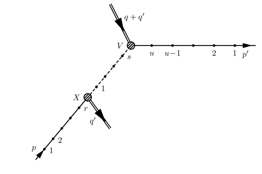
Figure 2: Defining the $p^{\prime}$ and $p$ legs for the process, $\chi\mathcal{F}\to\mathcal{F}\chi$. There are $r$ vertices on the $p$ leg, of which $w$ are on the initial fermion line.

As in GY, we consider the $n^{\rm th}$ order graph of Fig. 2 and begin by considering the insertion of an $(n+1)^{\rm th}$ virtual photon to it. Note that the form of the photon propagator in the thermal case continues to be proportional to $g_{\mu\nu}$ in the thermal case as well, although otherwise more complex, and of $2\times 2$ form, as seen from Eq. 3 and Eq. A.5, thus enabling the separation into $K$ and $G$ photon contributions à la GY :

$$g_{\mu\nu} =\left\{\left[g_{\mu\nu}-b_{k}(p_{f},p_{i})\,k_{\mu}k_{\nu}\right]+\left[b_{k}(p_{f},p_{i})k_{\mu}k_{\nu}\right]\right\}~{},$$

$$\equiv\left\{\left[G\right]+\left[K\right]\right\}~{},$$ (8)

with

$$b_{k}(p_{f},p_{i})=\frac{1}{2}\left[\frac{(2p_{f}-k)\cdot(2p_{i}-k)}{((p_{f}-k)^{2}-m^{2})((p_{i}-k)^{2}-m^{2})}+(k\leftrightarrow-k)\right]~{}.$$ (9)

There are many ways in which the vertices $\mu$ and $\nu$ of the $(n+1)^{\rm th}$ photon can be inserted into the $n^{\rm th}$ order graph. This includes

1. the two vertices of the virtual photon being on different fermion lines,

2. both vertices of the virtual photon on either of the fermion lines,

3. both vertices on the intermediate scalar line, and

4. one of the vertices on either of the fermion lines and the other on the scalar line.

We consider each of these possibilities, starting with the insertion of a virtual $K$ photon in the next subsection, and the insertion of a $G$ photon in the subsequent one. The new results in this paper are essentially from the consideration of the $K$ photon insertions. The proof that the $G$ photon insertions are finite follows from the detailed discussions of the corresponding thermal scalar and fermionic theories in Refs. [1, 10] and are reproduced here in brief. Additionally, the case of insertion of real photons is also strightfoward and the old results apply.

3.3 Insertion of virtual $K$ photons

We consider an $n^{\rm th}$ order graph as depicted in Fig. 2 and its higher order correction through a virtual $K$ photon insertion with momentum $k$ leaving/entering the graph at vertices $\mu$/$\nu$ on the ($p_{f}$)/($p_{i}$) legs respectively. Here $p_{f}$ and $p_{i}$ can be one of $p^{\prime}$ and $p$. (We consider the real photon contributions later). We express the $n^{\rm th}$ order matrix element generically as,

$${\cal{M}}_{n}^{p_{f},p_{i}}={\cal{C}}_{u}^{{\rm fermion}~{}p^{\prime}}\times{\cal{C}}_{s}^{\rm scalar}\times{\cal{C}}_{r}^{{\rm fermion}~{}p}~{},$$ (10)

where the subscripts on the right hand side simply denote the number of photon legs attached to the subdiagram. The first term includes the contribution of the fermion line from the final state fermion to the initial state bino, including vertex $V$; the second term contains the contributions of the scalar propagator between vertices $V$ and $X$, and the third term contains the contribution of the fermion line from the final bino to the initial fermion, including vertex $X$.

There are three possible types of insertion of the two vertices of the $(n+1)^{\rm th}$ $K$ photon, depending on the location where the vertices are inserted as listed above.

• While the insertion of both $\mu$ and $\nu$ vertices on the $p^{\prime}$ leg is analogous to the case studied by Grammer and Yennie, the other two cases differ.

• This is because the insertion with one vertex on the $p^{\prime}$ and one on the $p$ leg includes two possibilities, one where the $\nu$ vertex on the $p$ leg is on the scalar line and the other where it is on the initial fermion line (with the $\mu$ vertex being on the $p^{\prime}$ line in both cases).

• Similarly, the case where both $\mu$ and $\nu$ vertices are inserted on the $p$ leg includes three possibilities, viz., both vertices on the scalar line, both vertices on the fermion line, and one on each. Where both vertices are inserted on the same line, care must be taken to avoid double-counting by ordering the vertices.

We see that the case of thermal dark matter is a combination of thermal fermionic and scalar contributions. The effect of inserting a virtual $K$ photon in all possible ways on a fermion and scalar line were considered in detail in Refs. [10] and [1] respectively; we will use these results to compute the contributions for the dark matter interaction at hand. For the sake of completeness, we give the main highlights of these results in the next section.

3.3.1 Insertion of virtual $K$ photon vertices into a fermion or scalar line

In both cases, the process considered was the $2\to 1$ process $\varphi(p)\gamma^{*}(q)\to\varphi(p^{\prime})$ where $\varphi$ is appropriately a charged fermion or a charged scalar. Consider an $n^{\rm th}$ order graph with some number of real and virtual photon corrections, and consider the effect of adding an $(n+1)^{\rm th}$ virtual $K$ photon in all possible ways. The starting point is to consider the effect of inserting a single $\mu$ vertex of the virtual $K$ photon adjacent to an arbitrary vertex $q$ on both a fermion and scalar line and then add all possible permutations. Details can be found in Refs. [1, 10]. The main points to note are the following:

1. The insertion of a single vertex $\mu$ of a virtual $K$ photon on a fermion line gives rise to a difference of two terms in the thermal case, just as in GY at $T=0$. We have (see Eq. B.2 in Appendix B), for an insertion of vertex $\mu$ between vertices $q$ and $q+1$,

   $${\cal{M}}_{n+1}\propto ~{}~{}\bar{u}_{p^{\prime}}\gamma_{\mu_{1}}\cdots\gamma_{\mu_{q-1}}S^{q\mu}_{p^{\prime}+\sum_{q}}\,\not{k}\,S^{\mu,q+1}_{p^{\prime}+\sum_{q}+k}\cdots\Gamma_{V}u_{q+q^{\prime}}~{},$$

   $$\propto\bar{u}_{p^{\prime}}\gamma_{\mu_{1}}\cdots\gamma_{\mu_{q-1}}\left[S^{q,q+1}_{p^{\prime}+\sum_{q}}\delta_{t_{\mu},t_{q}+1}-S^{q,q+1}_{p^{\prime}+\sum_{q}+k}\delta_{t_{\mu},t_{q}}\right]~{}\cdots\Gamma_{V}u_{q+q^{\prime}}~{}.$$ (11)

   Here, the propagators $S$ correspond to fermions. The contributions when the vertex is inserted in all possible ways on a fermion line cancel term by term in pairs, leaving behind two terms, one which contains a factor $p^{\prime 2}-m^{2}$ which vanishes, and the other which is proportional to the lower order matrix element (see Ref. [10] for details). Symbolically, the contributions can be expressed as a sum of $s+1$ terms with $\mu$ inserted to the left of the vertex labelled $s$, to the left of vertex $s-1$, etc., all the way to the graph with $\mu$ inserted to the right of the vertex $1$. We have,

   $${\cal{M}}_{n+1}^{p^{\prime},\mu}\sim =\left\{(p^{\prime 2}-m_{f}^{2})\times M_{0}+M_{1}\right\}$$

   $$+\left\{M_{2}-M_{1}\right\}+\left\{\cdots\right\}+\left\{M_{s}-M_{s-1}\right\}+\left\{M_{s+1}-M_{s}\right\}~{}.$$ (12)

   This demonstrates the term by term cancellation. The left over term is

   $$M_{s+1}= \bar{u}_{p^{\prime}}\gamma_{1}S^{t_{1},t_{2}}_{p^{\prime}+\sum_{1}}\cdots S^{t_{s},t_{V}}_{p^{\prime}+\sum_{s}}\,\delta_{t_{\mu},t_{V}}\cdots~{},$$ (13)

   and is proportional to the lower order matrix element, along with the thermal factor $\delta_{t_{\mu},t_{V}}$. Since the hard vertex is an external one, $t_{V}=1$.

2. The insertion of a single vertex $\mu$ on a charged scalar line has two possibilities: one that the vertex is a new insertion on that line, leading to the formation of a new 3-point vertex. In this case too (see Eq. B.3 of Appendix B), the result is the difference of two terms. However, another possibility exists, viz., that the photon is inserted at an already existing vertex, converting the existing 3-point vertex to a 4-point vertex, an option that does not exist for fermionic QED. A simplification occurs when the contributions from the insertion of the $\mu$ vertex to the right of the vertex $q$ and that from the insertion of the $\mu$ vertex at the vertex $q$ are added together to form a so-called “circled vertex” [1], denoted ${}_{q}\mu$. The resulting contribution is again a difference of two terms, although not as simple and clean a factorisation:

   $${\cal M}_{n+1}^{q\mu,{\rm tot}}= ~{}S^{t_{V},t_{s}}_{P+\sum_{s}}\cdots\left[S^{t_{q-1},t_{q}}_{P+\sum_{q-1}}\delta_{t_{\mu},t_{q}}\left(2P+2\Sigma_{q-1}+l_{q}\right)_{\mu_{q}}\right.$$

   $$\left.-S^{t_{q-1},t_{q}}_{P+\sum_{q-1}+k}\delta_{t_{\mu},t_{q-1}}\left(2P+2\Sigma_{q-1}+2k+l_{q}\right)_{\mu_{q}}\right]S^{t_{q},t_{q+1}}_{P+\sum_{q}+k}\cdots S^{t_{1},t_{X}}_{P+\sum_{1}+k}~{},$$ (14)

   where $P\equiv p-q^{\prime}+\Sigma_{r}$ is the momentum to the right of vertex $X$. Here each $S$ corresponds to the scalar propagator with the appropriate thermal indices and momentum. This is the result for scalar thermal QED corresponding to Eq. 11 above for the fermionic case. Again, inserting the vertex $\mu$ in all possible ways on the scalar line gives contributions that cancel term by term giving rise to a great deal of simplification and a result that is similar to Eq. 12. An examination of the thermal factors shows that the left-over term arises from the insertion of the virtual $K$ photon vertex adjacent to the hard vertex $V$.

   Note that, in contrast to the initial and final fermion lines which have an outermost component that is on-shell (with momenta $p$ and $p^{\prime}$ respectively), neither end of the scalar line is on-shell. Hence, the earlier results on thermal scalar QED [1] need to be modified to bring back the terms proportional to $P^{2}-m^{2}$ that vanished in the earlier calculation. In the calculation that follows we therefore list separately the “on-shell” contribution that was already calculated in the earlier papers, as well as the new “off-shell” contribution due to these changes.

3. In the case when both $\mu$ and $\nu$ vertices are on the same leg, they are ordered with $\nu$ always to the left of $\mu$, to avoid double counting. In addition, for scalars, it is possible that two photons are inserted at the same vertex, giving rise to 4-point seagull vertices, in contrast to the fermionic case where only 3-point vertices exist. When both $\mu$ and $\nu$ vertices are inserted at the same point, we get 4-point tadpole diagrams, which again do not exist for fermions. This is the most complex case of all. We do not highlight details of this calculation but simply refer the reader to the original papers [1, 10]. We note only that the cancellation occurs again, leaving behind a term that is proportional to the lower order matrix element, but in this case the corresponding thermal factors of the left-over term are $\delta_{t_{\mu},t_{1}}\delta_{t_{\nu},t_{1}}$.

4. We summarise and highlight the dependence on the thermal factors as follows. When the vertices of the $(n+1)^{\rm th}$ $K$ photon are on different legs, the thermal factor of the left-over term that is proportional to the lower order matrix element depends on the thermal type of the hard vertex $V$, viz., $\delta_{t_{\mu},t_{V}}\delta_{t_{\nu},t_{V}}$. When the vertices of the $(n+1)^{\rm th}$ $K$ photon are on the same ($p^{\prime}$ or $p$) leg, the thermal factor of the left-over term that is proportional to the lower order matrix element depends on the thermal type of the outermost line of that leg (with momentum $p^{\prime}$ or $p$ respectively), viz., $\delta_{t_{\mu},t_{1}}\delta_{t_{\nu},t_{1}}$. The hard vertex $V$ involves participation of external/observable particles; the outermost lines of $p$ and $p^{\prime}$ legs are external lines as well; hence both are of thermal type 1. Thus the term that survives picks out only the (11) component of the inserted photon propagator, $i{\cal D}^{ab}_{\mu\nu}(k)$. This is critical to achieve cancellation of IR divergent terms between the virtual and real photon contributions.

We will now apply these results to examine the contributions to the graph in Fig. 2. We begin with the case when the two vertices are on the $p^{\prime}$ leg.

3.3.2 Insertion of both vertices of the virtual $K$ photon on the $p^{\prime}$ leg

This is the most straightforward part of the calculation and simply follows from the results for insertion of the $(n+1)^{\rm th}$ $K$-photon on the $p^{\prime}$ leg as given in Ref. [10] which deals with thermal fermionic QED. Both vertices are inserted in all possible ways in the lower order graph, keeping $\nu$ always to the left of $\mu$ in order to avoid double counting. The resulting contribution from all possible symmetric contributions is a term proportional to the lower order matrix element. Since the insertion only affects the $p^{\prime}$ leg, the parts of the matrix element involving the scalar and initial fermion $p$ legs are unchanged and we get,

$${\cal M}^{p^{\prime}p^{\prime},K\gamma}_{n+1}=+ie^{2}\int\frac{{\rm d}^{4}k}{(2\pi)^{4}}\,\delta_{t_{\mu},t_{1}}\,\delta_{t_{\nu},t_{1}}\,b_{k}(p^{\prime},p^{\prime})\,D^{t_{\mu},t_{\nu}}(k)~{}{\cal M}_{n}~{}.$$ (15)

Since $t_{1}=1$ necessarily, it depends only on the $D^{11}$ photon propagator, as before.

3.3.3 Insertion of virtual $K$ photon vertices separately on $p^{\prime}$ and $p$ legs

We now consider the case when the $\mu$ vertex is inserted on the $p^{\prime}$ leg and the $\nu$ vertex is inserted on the $p$ leg. The matrix element can be represented as,

$${\cal{M}}_{n+1}^{p^{\prime},p}\sim{\cal{C}}_{u+1}^{{\rm fermion}~{}p^{\prime},\mu}\times{\cal{C}}_{r+s+1}^{p,\nu}~{}.$$ (16)

Again, the subscript simply indicates the number of photon legs on the corresponding subdiagram, while the superscripts indicate the location where the vertices $\mu$ and $\nu$ are inserted.

3.3.3.1 Insertion of the $\mu$ vertex on the $p^{\prime}$ leg

The contributions from inserting $\mu$ on the $p^{\prime}$ leg and $\nu$ on the $p$ leg factorise and can be separately considered. The contribution from inserting a single vertex $\mu$ from a $K$ photon insertion on the fermion $p^{\prime}$ leg has been considered in detail in Ref. [10] and is proportional to the insertion of a factor $/{\!\!\!k}$ at the $\mu$ vertex; see Eq. 11 above. On including all possible insertions, the contributions cancel term by term in pairs, leaving behind only one term. The relevant part of the matrix element involving only the $p^{\prime}$ leg and the vertex $\mu$, inserted on it in all possible ways is given by,

$${\cal{C}}_{u+1}^{{\rm fermion}~{}p^{\prime},\mu}\sim\bar{u}_{p^{\prime}}\gamma_{\mu_{1}}S^{t_{1}t_{2}}_{p^{\prime}+\sum_{1}}\cdots(\hbox{no }k)\cdots S^{t_{s}t_{V}}_{p^{\prime}+\sum_{s}}\,\delta_{t_{\mu},t_{V}}\,\Gamma_{V}\,u_{q+q^{\prime}}~{},$$ (17)

where “no $k$” implies that all the corresponding terms have no $k$ dependence in them; $\Gamma_{V}$ represents the fermion-bino-scalar vertex. Here we have suppressed various overall factors for clarity and will put them back later. Hence we see that apart from the thermal factor $\delta_{t_{\mu},t_{V}}$, this part of the ${\cal{M}}_{n+1}$ matrix element is proportional to the corresponding part of the lower order matrix element, ${\cal{M}}_{n}$.

3.3.3.2 Insertion of the $\nu$ vertex on the $p$ leg

There are two contributions:

1. Insertion of the vertex $\nu$ on the scalar line,

2. Insertion of the vertex $\nu$ on the inital fermion line.

We denote their contributions to the resulting matrix element as,

$${\cal{C}}_{r+s+1}^{p,\nu}\sim\left[{\cal{C}}_{s+1}^{{\rm scalar},\nu}\times{\cal{C}}_{r}^{{\rm fermion}~{}p}(q_{i})+{\cal{C}}_{s}^{\rm scalar}(q_{i}\to q_{i}+k)\times{\cal{C}}_{r+1}^{{\rm fermion}~{}p,\nu}\right]~{}.$$ (18)

When the $\nu$ vertex is inserted on the initial fermion line, the momentum $k$ flows through the entire scalar line from the initial to the final fermion lines, but otherwise there are no new insertions on the scalar line. Hence the only effect of inserting the additional virtual photon on the fermion line is that every momentum on the scalar line is shifted by an additional factor, $k$, so that this portion of the matrix element is the same as the relevant lower order matrix element with shifted momenta:

$${\cal{C}}_{s}^{\rm scalar}={\cal{C}}_{s}^{\rm scalar}(q_{i}\to q_{i}+k)~{}.$$ (19)

When the $\nu$ vertex is inserted on the scalar line, the initial fermion line remains unaffected, since the additional momentum $k$ does not flow through it. Hence every intermediate propagator, $q_{i}$, remains the same as in the lower order graph, and the relevant portion of this matrix element is in fact the same as that of the lower order graph:

$${\cal{C}}_{r}^{{\rm fermion}~{}p}={\cal{C}}_{r}^{{\rm fermion}~{}p}(q_{i}\to q_{i})~{}.$$ (20)

The remaining terms in Eq. 18 are calculated below.

3.3.3.3 Insertion of the $\nu$ vertex of virtual $K$ photon on the scalar line

The contribution from inserting the $\nu$ vertex from a virtual $K$ photon insertion on the scalar part of the $p$ leg has been discussed in detail in Ref. [1]. For convenience, we relabel the momenta of the lines between the vertices $V$ and $X$ as $P+\Sigma_{s}$, $P+\Sigma_{s-1}$, $\cdots$, $P+\Sigma_{1}$ respectively, with $P\equiv p-q^{\prime}+\Sigma_{r}$ being the momentum of the propagator to the right of the vertex $X$, where $k_{1},k_{2},\ldots,k_{r}$ are the photon momenta entering the $r$ vertices on the $p$ fermion leg.

The major difference between the earlier calculation and this one is that here the scalar line is completely off-shell, unlike earlier, where it was either the final or initial leg, with the outermost line on-shell. Hence we have to account for this difference in the current calculation. Apart from the inclusion of the scalar propagator between the vertices $1$ and $X$ since this line is no longer on-shell, we must take into account the fact that $P$ itself is off-shell. Hence, a term in the earlier calculation for scalar QED which vanished because $P^{2}=m^{2}$ is now not zero. We get,

$${\cal{C}}_{s+1}^{{\rm scalar},\nu} \sim S^{t_{X},t_{1}}_{P}(2P+l_{1})_{\mu_{1}}S^{t_{1},t_{2}}_{P+\sum_{1}}\cdots S^{t_{s},t_{V}}_{P+\sum_{s}}\left[\delta_{t_{\nu},t_{V}}\right]$$

$$~{}~{}~{}~{}~{}-S^{t_{X},t_{1}}_{P+k}(2P+2k+l_{1})_{\mu_{1}}\cdots S^{t_{s},t_{V}}_{P+k+\sum_{s}}\left[\delta_{t_{\nu},t_{X}}\right]~{}.$$ (21)

The first term has no $k$ dependence and is therefore proportional to the corresponding part of the lower order matrix element; note that this contribution would have vanished if $P$ was on-shell. We see that there is an extra term, with $k$ dependence in each part of the contribution, which arises when the $\nu$ vertex is just to the right of vertex $X$. In contrast to the corresponding result in Ref. [1] where this contribution was independent of $k$ and proportional to the lower order matrix element, here every momentum is shifted by $k$ since this momentum runs through practically the entire scalar leg, from the vertex $V$ to the vertex $\nu$ just to the left of $X$. We will see below that this extra term cancels against the contribution when the $\nu$ vertex is inserted on the fermion $p$ line.

3.3.3.4 Insertion of the $\nu$ vertex of the virtual $K$ photon on the fermion $p$ line

The contribution from inserting a single vertex $\nu$ from a virtual $K$ photon insertion on the fermionic part of the $p$ leg has been calculated in Ref. [10]; since the outermost leg is on-shell, $p^{2}=m^{2}$, we can apply the earlier results with just the replacement of the appropriate vertex factor at the vertex $X$. As before, terms from all possible insertions of this vertex cancel in pairs, and we have,

$${\cal{C}}_{r+1}^{{\rm fermion}~{}p,\nu}\sim\bar{u}_{q^{\prime}}\Gamma_{X}S^{t_{X}t_{r}}_{p+\sum_{r}}\delta_{t_{\nu},t_{X}}\gamma_{r}\cdots(\hbox{no }k)~{}u_{p}~{},$$ (22)

with the corresponding scalar contribution having the factor $k$ added to the momentum of each propagator: $q_{i}\to q_{i}+k$, as mentioned in Eq. 19 above. Both these insertions contribute to the matrix element in Eq. 18. Substituting, Eq. 18 simplifies due to cancellations as shown below to,

$${\cal{C}}_{r+s+1}^{p,\nu} \sim\left[\left\{S^{t_{X},t_{1}}_{P}(2P+l_{1})_{\mu_{1}}S^{t_{1},t_{2}}_{P+\sum_{1}}\cdots S^{t_{s},t_{V}}_{P+\sum_{s}}\left[\delta_{t_{\nu},t_{V}}\right]\right.\right.$$

$$~{}~{}~{}~{}~{}\left.-S^{t_{X},t_{1}}_{P+k}(2P+2k+l_{1})_{\mu_{1}}\cdots S^{t_{s},t_{X}}_{P+k+\sum_{s}}\left[\delta_{t_{\nu},t_{X}}\right]~{}\right\}\times\left\{\bar{u}_{q^{\prime}}\Gamma_{X}S^{t_{X},t_{r}}_{p+\sum_{r}}\gamma_{r}\cdots(\hbox{no }k)~{}u_{p}\right\}$$

$$~{}~{}~{}~{}~{}+\left.\left\{S^{t_{X},t_{1}}_{P+k}(2P+2k+l_{1})_{\mu_{1}}\cdots S^{t_{s},t_{V}}_{P+k+\sum_{s}}\right\}\times\left\{\bar{u}_{q^{\prime}}\Gamma_{X}S^{t_{X},t_{r}}_{p+\sum_{r}}\delta_{t_{\nu},t_{X}}\gamma_{r}\cdots(\hbox{no }k)~{}u_{p}\right\}\right]~{},$$

$$\sim\left\{S^{t_{X},t_{1}}_{P}(2P+l_{1})_{\mu_{1}}S^{t_{1},t_{2}}_{P+\sum_{1}}\cdots S^{t_{s},t_{V}}_{P+\sum_{s}}\left[\delta_{t_{\nu},t_{V}}\right]\right\}\times\left\{\bar{u}_{q^{\prime}}\Gamma_{X}S^{t_{X},t_{r}}_{p+\sum_{r}}\gamma_{r}\cdots(\hbox{no }k)~{}u_{p}\right\}~{}.$$ (23)

3.3.4 Matrix element for insertion of virtual $K$ photon on different legs

Substituting for Eqs. 23 and 17, ${\cal{M}}_{n+1}^{p^{\prime},p}$ in Eq. 16 evaluates to,

$${\cal{M}}_{n+1}^{p^{\prime},p}\sim \left\{\bar{u}_{p^{\prime}}\gamma_{\mu_{1}}S^{t_{1}t_{2}}_{p^{\prime}+\sum_{1}}\cdots(\hbox{no }k)\cdots S^{t_{s}t_{V}}_{p^{\prime}+\sum_{s}}\,\delta_{t_{\mu},t_{V}}\,\Gamma_{V}\,u_{q+q^{\prime}}\right\}\times$$

$$\left\{S^{t_{X},t_{1}}_{P}(2P+l_{1})_{\mu_{1}}S^{t_{1},t_{2}}_{P+\sum_{1}}\cdots S^{t_{s},t_{V}}_{P+\sum_{s}}\left[\delta_{t_{\nu},t_{V}}\right]\right\}\times\left\{\bar{u}_{q^{\prime}}\Gamma_{X}S^{t_{X},t_{r}}_{p+\sum_{r}}\gamma_{r}\cdots(\hbox{no }k)~{}u_{p}\right\}~{},$$

$$\propto{\cal{M}}_{n}\times\left[\delta_{t_{\mu},t_{V}}\right]\,\left[\delta_{t_{\nu},t_{V}}\right]~{};$$ (24)

hence the total contribution is proportional to the lower order matrix element. Note that the propagators may correspond to either fermion or scalar ones, as appropriate. Putting back the overall factors, including parts of the photon propagator that had been omitted, we have,

$${\cal M}^{p^{\prime}p,K\gamma}_{n+1} =-ie^{2}\int\frac{{\rm d}^{4}k}{(2\pi)^{4}}\,\delta_{t_{\mu},t_{V}}\,\delta_{t_{\nu},t_{X}}b_{k}(p^{\prime},p)D^{t_{\mu},t_{\nu}}(k)\times{\cal M}_{n}~{}.$$ (25)

Note that for thermal QED we had obtained [10, 1] thermal terms that were proportional to $\delta_{t_{\mu},t_{V}}\delta_{t_{\nu},t_{V}}D^{t_{\mu},t_{\nu}}(k)$, and hence to the (11) element of the thermal photon propagator, $D^{11}(k)$, since there was a single hard vertex, $V$. We obtain a similar result here as well, since the bino particles at both the $V$ and $X$ vertices are external particles and hence of thermal type-1; that is, the matrix element is again proportional to the (11) element of the photon propagator, $D^{11}(k)$, as before. This result also holds for arbitrary number of intermediate scalar and fermion propagators on the $p$ leg (with arbitrary corresponding emissions of bino particles at each of these vertices) since the bino is always on-shell.

3.3.4.1 Discussion on the nature of the cancellation

In the case where both the vertices of the $(n+1)^{\rm th}$ photon are inserted on the $p^{\prime}$ leg, the term-by-term cancellation, leaving behind just one term proportional to the lower order matrix element, as shown in Eq. 15, occurs just as in the case of thermal fermionic QED discussed in Ref. [10]. However, when the two vertices are inserted on different legs, the result shown in Eqs. 23 and 24 involves a double cancellation. This can be understood as follows. The $\mu$ vertex insertion on the $p^{\prime}$ leg is straightforward. However, there are two parts to the $p$ leg, viz., the scalar propagator, and the initial fermion $p$ line. A set of term-by-term cancellations occurs when the $\nu$ vertex is inserted in all possible ways on the fermion $p$ line. However, even though this part of the matrix element is then proportional to the lower order matrix element, the part of the matrix element from the scalar propagator that multiplies this, contains the $k$ dependence since this extra momentum flows through it. On the other hand, the contribution when the $\nu$ vertex is inserted in all possible ways on the scalar propagator has a term by term cancellation, leaving behind two terms. Due to the presence of the thermal indices, it is easy to see from Eq. 21 that one term arises from the $\nu$ insertion adjacent to vertex $V$ and the other one from an insertion adjacent to vertex $X$. We know from the discussion in Section 3.3.1 that insertions on two different legs (in the purely fermionic or purely scalar case) results in a term that is proportional to $\delta_{t_{\nu},t_{V}}$. The fact that there is an additional term with $\delta_{t_{\nu},t_{X}}$ indicates the incomplete cancellation owing to the relevant momentum (to the right of vertex $X$) not being on-shell. All possible insertions of $\nu$ on the remaining part of the $p$ leg, viz., on the fermionic $p$ line, allow a term by term cancellation that leaves just one term. As per the discussion in Section 3.3.1, this should arise from insertion adjacent to the hard vertex which is $X$ in this case. Hence the corresponding term is proportional to the thermal factor $\delta_{t_{\nu},t_{X}}$ and this term cancels the left-over term from all possible insertions on the scalar part of the $p$ leg.

It can also be seen that nowhere was the exact form of the bino vertex required, either at vertex $V$ or vertex $X$. The term-by-term cancellation occurs independently of the exact nature of this interaction. Hence the analysis is “blind” to the precise structure of the hard process at vertices $V$ and $X$.

3.3.5 Insertion of both vertices of the virtual $K$ photon on the $p$ leg

Since the $p$ leg comprises both the scalar line as well as the initial fermion line, this is the most complex part of the calculation and has three components with three different types of insertion of the vertices of the virtual $K$ photon:

1. Both vertices on the fermion $p$ line,

2. One vertex on the scalar line and one on the fermion $p$ line,

3. Both vertices on the intermediate scalar line.

Since the contribution from the $p^{\prime}$ leg is unaffected by the insertion, we denote these contributions as

$${\cal{M}}_{n+1}^{p,p} \sim{\cal{C}}_{u}^{{\rm fermion}~{}p^{\prime}}\times\left[{\cal{C}}_{s}^{\rm scalar}\times{\cal{C}}_{r+2}^{{\rm fermion}~{}p;\mu,\nu}+{\cal{C}}_{s+1}^{\rm scalar;\mu}\times{\cal{C}}_{r+1}^{{\rm fermion}~{}p;\nu}\right.$$

$$~{}~{}~{}~{}~{}~{}~{}~{}~{}~{}~{}\left.+{\cal{C}}_{s+2}^{{\rm scalar};\mu,\nu}\times{\cal{C}}_{r}^{{\rm fermion}~{}p}\right]~{}.$$ (26)

We will study each in turn. Again, we highlight that neither of the outermost legs of the scalar line is on shell; hence we have to bring back the terms which were dropped on account of setting $P^{2}-m^{2}=0$. We refer to these extra terms as “off-shell” contributions that occur over and above the earlier results which are labelled as the “on-shell” part. We also have to include the propagator corresponding to the outermost part of the scalar line as an overall multiplicative factor for all terms since it is not on-shell; this is a trivial modification.

We begin with the insertion of both vertices on the fermion part of the $p$ leg.

3.3.5.1 Insertion of both $\mu$, $\nu$ vertices of the $K$ photon on the fermionic $p$ leg

This involves inserting both vertices of the virtual $K$ photon on a fermion line having $r$ vertices, in all possible ways. There is no $k$ dependence in the rest of the diagram (the final $p^{\prime}$ leg or the intermediate scalar line). This has been calculated in Ref. [10] for fermionic thermal QED and the result is proportional to the lower order matrix element. However, as per GY, we have to remove a term corresponding to the insertion of $\nu$ and $\mu$ just to the right of vertex $1$ on the fermion line, to account for wave function renormalisation. Hence the net contribution of this insertion is zero, as was the corresponding case for purely fermionic thermal QED [10]:

$${\cal{C}}_{r+2}^{{\rm fermion}~{}p;\mu,\nu} =0~{};$$

$$\hbox{Hence, }{\cal{C}}_{s}^{\rm scalar}\times{\cal{C}}_{r+2}^{{\rm fermion}~{}p;\mu,\nu} =0~{}.$$ (27)

3.3.5.2 Insertion of the $\mu$ vertex of the $K$ photon on the scalar part and the $\nu$ vertex on the fermionic part of the $p$ leg

As in the case when the $\nu$ vertex was on the fermionic $p$ leg and the $\mu$ vertex is on the scalar leg, the contributions due to the two vertex insertions factorise and can be independently calculated.

For the scalar line, the $\mu$ vertex is again inserted in all possible ways on the scalar line. There are $s+1$ contributions, as discussed in Ref. [1], with $s$ diagrams each having one circled vertex, ${}_{q}\mu$, $q=1,\cdots s$, and one diagram with vertex $\mu$ inserted to the right of vertex $X$; see Ref [1]. Again we note that neither end of the scalar line is on-shell. The contributions from each insertion can be written as a difference of two terms, analogous to the fermionic result in Eq. 12,

$${\cal{C}}_{s+1}^{{\rm scalar};\mu} = \left\{\left[S^{t_{V},t_{1}}_{P}\delta_{t_{\mu},t_{1}}(2P+l_{1})_{\mu_{1}}-S^{t_{V},t_{1}}_{P+k}\delta_{t_{\mu},t_{V}}(2P+2k+l_{1})_{\mu_{1}}\right]\right.\times$$ (28)

$$\left.~{}~{}~{}~{}~{}~{}~{}~{}S^{t_{1},t_{2}}_{P+\sum_{1}+k}(2P+2k+2\Sigma_{1}+l_{2})_{\mu_{2}}\cdots\right\}$$

$$+\left\{S^{t_{V},t_{1}}_{P}(2P+l_{1})_{\mu_{1}}\left[S^{t_{1},t_{2}}_{P+\sum_{1}}\delta_{t_{\mu},t_{2}}(2P+2\Sigma_{1}+l_{2})_{\mu_{2}}\right.\right.$$

$$~{}~{}~{}~{}~{}~{}~{}~{}\left.\left.-S^{t_{1},t_{2}}_{P+\sum_{1}+k}\delta_{t_{\mu},t_{1}}(2P+2\Sigma_{1}+2k+l_{2})_{\mu_{2}}\right]\cdots\right\}$$

$$+\left\{\cdots\right\}$$

$$+\left\{S^{t_{V},t_{1}}_{P}(2P+l_{1})_{\mu_{1}}S^{t_{1},t_{2}}_{P+\sum_{1}}\cdots\left[S^{t_{s-1},t_{s}}_{P+\sum_{s-1}}\delta_{t_{\mu},t_{s}}(2P+2\Sigma_{s-1}+l_{s})_{\mu_{s}}\right.\right.$$

$$\left.\left.+S^{t_{s-1},t_{s}}_{P+\sum_{s-1}+k}\delta_{t_{\mu},t_{s-1}}(2P+2\Sigma_{s-1}+2k+l_{s})_{\mu_{s}}\right]\cdots\right\}$$

$$+\left\{S^{t_{V},t_{1}}_{P}(2P+l_{1})_{\mu_{1}}S^{t_{1},t_{2}}_{P+\sum_{1}}\cdots\left[S^{t_{s},t_{X}}_{P+\sum_{s}}\delta_{t_{\mu},t_{X}}-S^{t_{s},t_{X}}_{P+\sum_{s}+k}\delta_{t_{\mu},t_{s}}\right]\right\}~{},$$

$$\equiv \left\{M_{1}-M_{0}\right\}+\left\{M_{2}-M_{1}\right\}+\left\{\cdots\right\}+\left\{M_{s}-M_{s-1}\right\}+\left\{M_{s+1}-M_{s}\right\}~{}.$$

It is seen that the terms cancel in pairs, leaving behind two terms, $M_{0}$ and $M_{s+1}$. In contrast, the result when a single vertex $\mu$ was inserted in all possible ways on a scalar leg with the external leg having a momentum $P$ for purely thermal scalar fields [1], it was found to be proportional to just the $M_{s+1}$ term (without the initial factor, $S^{t_{V},t_{1}}_{P}$); the $M_{0}$ term evaluated to zero since $P$ was on-shell.

This factor is multiplied by the part of the matrix element arising from the fermion part of the $p$ leg. Applying the generalised Feynman identities defined in Appendix B, insertion of the $\nu$ vertex in all possible ways into the fermionic part of the $p$ leg gives sets of terms that cancel against each other. This has been calculated in the thermal fermionic QED case in Ref. [10]; we simply use the result obtained in this paper to get,

$${\cal{C}}_{r+1}^{{\rm fermion}~{}p;\nu}\sim\left\{\bar{u}_{q^{\prime}}\Gamma_{X}S^{t_{X},t_{r}}_{p^{\prime}+\sum_{r}}\delta_{\nu,X}\gamma_{r}\cdots(\hbox{no }k)~{}u_{p}~{}\right\}~{}.$$ (29)

This is again proportional to the corresponding part of the lower order matrix element since it is independent of $k$. Combining both terms, we obtain the product,

$${\cal{C}}_{s+1}^{\rm scalar;\mu}\times{\cal{C}}_{r+1}^{{\rm fermion}~{}p;\nu} \sim \left[-S^{t_{V},t_{1}}_{P+k}~{}\delta_{t_{\mu},t_{V}}(2P+2k+l_{1})_{\mu_{1}}\right.\times$$ (30)

$$\left.~{}~{}~{}~{}~{}~{}~{}~{}S^{t_{1},t_{2}}_{P+\sum_{1}+k}(2P+2k+2\Sigma_{1}+l_{2})_{\mu_{2}}\cdots\right.$$

$$+\left.S^{t_{V},t_{1}}_{P}(2P+l_{1})_{\mu_{1}}S^{t_{1},t_{2}}_{P+\sum_{1}}\cdots S^{t_{s},t_{X}}_{P+\sum_{s}}~{}\delta_{t_{\mu},t_{X}}\right]~{}$$

$$\times\left\{\bar{u}_{q^{\prime}}\Gamma_{X}S^{t_{X},t_{r}}_{P+\sum_{r}}~{}\delta_{\nu,X}\gamma_{r}\cdots(\hbox{no }k)u_{p}~{}\right\}~{}.$$

The term corresponding to $M_{0}$ in the earlier calculation was zero owing to the presence of the term $P^{2}-m^{2}=0$. Note that $M_{s+1}$ is independent of $k$ so that its contribution is proportional to the lower order matrix element; however, the extra term $M_{0}$ is not, and so the factorisation is not yet obtained.

3.3.5.3 Insertion of both $\mu$, $\nu$ vertices of the $K$ photon on the scalar part of the $p$ leg

As in the case of pure scalar thermal QED, this is a more involved calculation since there are both 3-point and 4-point vertices for scalars; also, apart from seagull-type insertions with 2-scalar-2-photon lines at a vertex, there can also be tadpole-type diagrams with the two photon lines at the vertex forming a loop. We will briefly outline and use the results obtained earlier in Ref. [1] and merely highlight the extra “off-shel” contributions. As discussed in Ref. [1], there are four sets of contributing diagrams:

1. Set I, with circled vertices ${}_{q}\mu$ and ${}_{q}\nu$ at both $\mu$ and $\nu$ insertions, where $q$ are any of the already existing vertices, $q=1,\cdots,s$.

2. Set II, with circled vertices ${}_{q}\mu$ only at $\mu$, with $\nu$ to the right of the special vertex, $X$.

3. Set III, with all 4-point vertex insertions of $\nu$, so that $\nu$ is inserted at any of the already existing $q$ vertices, $q=\nu$, with $\mu$ immediately adjacent to $\nu$.

4. Finally, Set IV, which is a set of ${}_{\nu}\mu$ circled vertices that includes all tadpole insertions, $\mu=\nu$, as well.

Note that the calculation in Ref. [1] was for insertions on the scalar $P$ leg where the external leg, $P$ was on-shell. Here this is not the case here and this gives rise to extra contributions. It turns out that it is possible to express the result of these contributions as the sum of two parts: one, which is the same as the result in Ref. [1] (with the usual additional propagator prefactor $S^{t_{V},t_{1}}_{p^{\prime}}$), referred to as the “on-shell” contribution, and the second, which are the terms arising from the fact that $P$ is not on-shell which we label the “off-shell” contribution. Note that this is simply a convenient assignment; all terms of the part labelled “on-shell” are not explicitly dependent on $P$ being on-shell; rather they are blind to the off-shell or on-shell nature of $P$. It is the “off-shell” part that arises strictly owing to the off-shell nature of $P$. We now explicitly list the extra contributions to the various sets below, and refer the reader to Ref. [1] for the “on-shell” contribution.

The contribution from Set I is given by,

$${\cal{C}}_{s+2}^{{\rm scalar};\mu,\nu,I} = S^{t_{V},t_{1}}_{P}\left\{{\hbox{On-shell}}\right\}$$ (31)

$$+S^{t_{V},t_{1}}_{P+k}~{}\delta_{t_{\mu},t_{V}}(2P+2k+l_{1})_{\mu_{1}}\left\{-S^{t_{1},t_{2}}_{P+\sum_{1}}~{}\delta_{t_{1},t_{\nu}}(2P+2\Sigma_{1}+l_{2})_{\mu_{2}}\cdots(\hbox{no }k)\right.$$

$$+\left.S^{t_{1},t_{2}}_{P+\sum_{1}+k}(2P+2\Sigma_{1}+2k+l_{2})_{\mu_{2}}\cdots(\hbox{all }k)~{}\delta_{t_{\nu},t_{s}}\right\}~{},$$

where “no $k$” and “all $k$” refer to the fact that none or all of the vertex and propagator terms in the sequence are $k$-dependent and the “off-shell” contributions only have been explicitly listed. Similarly, the contribution from Set II can be expressed as,

$${\cal{C}}_{s+2}^{{\rm scalar};\mu,\nu,II} = S^{t_{V},t_{1}}_{P}\left\{{\hbox{On-shell}}\right\}$$ (32)

$$-S^{t_{V},t_{1}}_{P+k}~{}\delta_{t_{\mu},t_{V}}(2P+2k+l_{1})_{\mu_{1}}S^{t_{1},t_{2}}_{P+\sum_{1}+k}(2P+2\Sigma_{1}+2k+l_{2})_{\mu_{2}}\cdots(\hbox{all }k)\times$$

$$\left[S^{t_{s},t_{X}}_{P+\sum_{s}}~{}\delta_{t_{\nu},t_{s}}-S^{t_{s},t_{X}}_{P+k+\sum_{s}}~{}\delta_{t_{\nu},t_{X}}\right]~{}.$$

The contribution from Set III can be expressed as,

$${\cal{C}}_{s+2}^{{\rm scalar};\mu,\nu,III} = S^{t_{V},t_{1}}_{P}\left\{{\hbox{On-shell}}\right\}$$ (33)

$$-S^{t_{V},t_{1}}_{P+k}~{}\delta_{t_{\mu},t_{V}}(-2k)_{\mu_{1}}~{}\delta_{t_{\nu},t_{1}}S^{t_{1},t_{2}}_{P+\sum_{1}}\cdots(\hbox{no }k)~{}S^{t_{s},t_{X}}_{P+\sum_{s}}~{}.$$

As in the case of pure scalar thermal QED [1], the tadpole contributions in Set IV cancel the $k^{2}$ dependent terms in the remaining part of Set IV. This is again crucial to the factorisation since $k^{2}$ terms are IR finite (both at zero and finite temperature) but will spoil the factorisation and subsequent exponentiation at all orders of the IR divergent coefficients. We have,

$${\cal{C}}_{s+2}^{{\rm scalar};\mu,\nu,IV} = S^{t_{V},t_{1}}_{P}\left\{{\hbox{On-shell}}\right\}$$ (34)

$$+~{}0~{}.$$

Note that the calculation in Ref. [1] did not include the self-energy correction diagrams on the outermost part of the $p$ scalar leg, to account for wave function renormalisation. Here, however, the scalar $P$ leg is off-shell. Adding back these terms to Set IV, we get,

$${\cal{C}}_{s+2}^{{\rm scalar};\mu,\nu,IV} = S^{t_{V},t_{1}}_{P}\left\{{\hbox{On-shell}}\right\}+~{}{\cal{M}}_{n+1}^{{\rm scalar};\mu,\nu,{\rm Self}}$$ (35)

$$= S^{t_{V},t_{1}}_{P}\left\{{\hbox{On-shell}}\right\}$$

$$+\left\{S^{t_{V},t_{\nu}}_{P}~{}\delta_{t_{\mu},t_{\nu}}(2P\cdot k)\,S^{t_{\nu},t_{1}}_{P}-~{}\delta_{t_{\mu},t_{V}}\left[S^{t_{V},t_{1}}_{P}~{}\delta_{t_{\nu},t_{V}}-S^{t_{V},t_{1}}_{P+k}~{}\delta_{t_{\nu},t_{1}}\right]\right\}\times$$

$$~{}~{}~{}~{}~{}~{}~{}~{}~{}~{}(2P+l_{1})_{\mu_{1}}\,S^{t_{1},t_{2}}_{P+\sum_{1}}\cdots(\hbox{ no }k)~{}.$$

As shown in Ref. [1], the original contribution has one term that is proportional to the lower order matrix element, as well as a tower of terms that contain only one term that depends on $k$ in the numerator; in particular this dependence is odd in $k$, being either $Q\cdot k$ or $(-2k)_{\mu_{q}}$, where $Q$ is a combination of the momenta not involving $k$: $Q=P+\sum_{q}$. The remaining $k$ dependence is contained in the overall integration $\int d^{4}k$, the term $b_{k}$, and the part of the photon propagator, $D^{t_{\mu},t_{\nu}}(k)$, all of which are symmetric in $(k\leftrightarrow-k)$. Hence such terms odd in $k$ vanish, leaving behind only the term that is otherwise $k$ independent and proportional to the lower order matrix element. Applying the result from Ref. [1], we have,

$$\left\{{\hbox{On-shell}}^{I+II+III+IV}\right\}= S^{t_{V},t_{1}}_{P}\left\{-~{}\delta_{t_{\mu},t_{1}}~{}\delta_{t_{\nu},t_{1}}(2P+l_{1})_{\mu_{1}}S^{12}_{P+\sum_{1}}(2P+2\Sigma_{1}+l_{2})_{\mu_{2}}\cdots\right\}~{},$$ (36)

and hence is proportional to the lower order matrix element as well as the expected thermal delta function factors for both insertions on the same leg (see Section 3.3.1). Note that in obtaining this result we have dropped terms that are linear in $k$ (such as $Q\cdot k$ and $(-2k_{\mu_{q}}$) since such odd terms vanish on integration. In addition, the $k^{2}$ dependence cancels on inclusion of the tadpole diagrams as was the case for pure scalar thermal QED.

Now, adding in the extra contributions from all four sets, we see that the contribution from Set III and the first term from Set I cancels the total contribution from Set IV (self energy terms); see Eqs. 31, 33, and 35. Also, the second term in Set I cancels the first term of Set II, leaving behind only the second term of Set II, which adds to the “on-shell” contribution, giving the total contribution from both insertions on the scalar part of the $p$ leg to be,

$${\cal{C}}_{s+2}^{{\rm scalar};\mu,\nu} \sim \left\{{\hbox{On-shell}}^{I+II+III+IV}\right\}+S^{t_{V},t_{1}}_{P+k}~{}\delta_{t_{\mu},t_{V}}(2P+2k+l_{1})_{\mu_{1}}\times$$ (37)

$$S^{t_{1},t_{2}}_{P+\sum_{1}+k}(2P+2\Sigma_{1}+2k+l_{2})_{\mu_{2}}\cdots(\hbox{all }k)\times S^{t_{s},t_{X}}_{P+k+\sum_{s}}~{}\delta_{t_{\nu},t_{X}}~{},$$

where the first term is given in Eq. 36. This result for insertion of both vertices on the scalar part of the $p$ leg, is to be multiplied with the contribution from the fermionic part of the $p$ leg; since this has no $k$ dependence, it is simply given by the corresponding part of the lower order matrix element. We have,

$${\cal{C}}_{s+2}^{{\rm scalar};\mu,\nu}\times{\cal{C}}_{r}^{{\rm fermion}~{}p} \sim \left\{-S^{t_{V},t_{1}}_{P}~{}\delta_{t_{\mu},t_{1}}~{}\delta_{t_{\nu},t_{1}}(2P+l_{1})_{\mu_{1}}S^{12}_{P+\sum_{1}}(2P+2\Sigma_{1}+l_{2})_{\mu_{2}}\cdots\right.$$ (38)

$$+S^{t_{V},t_{1}}_{P+k}~{}\delta_{t_{\mu},t_{V}}(2P+2k+l_{1})_{\mu_{1}}S^{t_{1},t_{2}}_{P+\sum_{1}+k}(2P+2\Sigma_{1}+2k+l_{2})_{\mu_{2}}$$

$$\left.\cdots S^{t_{s},t_{X}}_{P+k+\sum_{s}}~{}\delta_{t_{\nu},t_{X}}\right\}\times\left\{\bar{u}_{q^{\prime}}\Gamma_{X}S^{t_{X},t_{r}}_{p+\sum_{r}}~{}\delta_{\nu,X}\gamma_{r}\cdots u_{p}~{}\right\}~{}.$$

We now compute the total contribution when both vertices are inserted on the $p$ leg as the sum of contributions from the three different types of insertions, viz., both vertices on the fermion part of the $p$ leg, one vertex each on the fermion and scalar part of the $p$ leg, and both vertices on the scalar part of the $p$ leg (that is, the sum of Eqs. 27, Eqs. 30, and Eqs. 38). We find that the first term of Eq. 30 cancels against the second term of Eq. 38, while the contribution of Eq. 27 evaluated to zero. The final contribution is therefore,

$${\cal{M}}_{n+1}^{p,p} \sim \left\{S^{t_{V},t_{1}}_{P}(2P+l_{1})_{\mu_{1}}S^{t_{1},t_{2}}_{P+\sum_{1}}\cdots S^{t_{s},t_{X}}_{P+\sum_{s}}~{}\delta_{t_{\mu},t_{X}}-S^{t_{V},t_{1}}_{P}~{}\delta_{t_{\mu},t_{1}}~{}\delta_{t_{\nu},t_{1}}(2P+l_{1})_{\mu_{1}}S^{t_{1},t_{2}}_{P+\sum_{1}}\right.$$ (39)

$$\left.\cdots S^{t_{s},t_{X}}_{P+\sum_{s}}\right\}\times\left\{\bar{u}_{q^{\prime}}\Gamma_{X}S^{t_{X},t_{r}}_{p+\sum_{r}}~{}\delta_{\nu,X}\gamma_{r}\cdots u_{p}~{}\right\}~{},$$

$$= \left(\delta_{t_{\mu},t_{X}}\delta_{t_{\nu},t_{X}}-\delta_{t_{\mu},t_{1}}\delta_{t_{\nu},t_{1}}\right)\times\left\{S^{t_{V},t_{1}}_{P}(2P+l_{1})_{\mu_{1}}S^{t_{1},t_{2}}_{P+\sum_{1}}\cdots\right\}~{},$$

$$= 0~{},$$

since $t_{X}=t_{1}=1$.

3.3.5.4 Discussion on the nature of the cancellation

It is instructive to understand the origin of this result. Note that it is identical to the result from purely fermionic or purely scalar QED that contributions from insertions of both vertices of the virtual $(n+1)^{\rm th}$ $K$ photon on the $p$ leg in all possible ways vanishes. In the present case, there are three contributions. The one where both vertices are on the fermionic part of the $p$ leg is zero, as before. There are two more contributions, one where both vertices are on the scalar line and one where one vertex is on the scalar line and the other on the initial fermion line.

The contribution when one vertex each is on the scalar and fermion lines was expected to give a single contribution that is proportional to $\delta_{t_{\nu},t_{X}}\delta_{t_{\mu},t_{X}}$; however, due to the off-shell nature of the scalar line, there is an additional term proportional to $\delta_{t_{\nu},t_{X}}\delta_{t_{\mu},t_{V}}$ as well.

The contribution when both vertices are on the scalar line are terms proportional to $\delta_{t_{\nu},t_{1}}\delta_{t_{\mu},t_{1}}$ as expected from the discussion in Section 3.3.1; however, there is an additional term proportional to $\delta_{t_{\nu},t_{X}}\delta_{t_{\mu},t_{V}}$ arising from the off-shell nature of the scalar line. The extra terms in each of these two contributions cancel each other, leaving behind terms proportional to $\delta_{t_{\nu},t_{X}}\delta_{t_{\mu},t_{X}}$ and $\delta_{t_{\nu},t_{1}}\delta_{t_{\mu},t_{1}}$ which cancel against each other since the thermal factors of all external fields are the same, $t_{X}=t_{V}=t_{1}=1$. Hence the cancellation is non-trivial and cannot be written down just by inspection of the pure fermion or pure scalar case alone.

3.3.6 Final matrix element for both vertices of the $K$ photon on the same leg

As in the case of thermal QED, we can symmetrise this result since we could have accounted for wave function renormalisation either on the $p^{\prime}$ leg or on the $p$ leg. Putting back the suppressed factors such as $b_{k}(p,p)$, the remaining part of the photon propagator, and the integration over $k$, we have,

$${\cal M}^{p^{\prime}p^{\prime},K\gamma}_{n+1} = +\frac{ie^{2}}{2}\int\frac{{\rm d}^{4}k}{(2\pi)^{4}}\,\delta_{t_{\mu},t_{1}}\,\delta_{t_{\nu},t_{1}}\,b_{k}(p^{\prime},p^{\prime})\,D^{t_{\mu},t_{\nu}}(k)~{}{\cal M}_{n}~{};$$

$${\cal M}^{pp,K\gamma}_{n+1} = +\frac{ie^{2}}{2}\int\frac{{\rm d}^{4}k}{(2\pi)^{4}}\,\delta_{t_{\mu},t_{1}}\,\delta_{t_{\nu},t_{1}}\,b_{k}(p,p)\,D^{t_{\mu},t_{\nu}}(k)~{}{\cal M}_{n}~{}.$$ (40)

Eq. 40, along with Eq. 25 shows the factorisation of all possible insertions of an $(n+1)^{\rm th}$ virtual $K$ photon into an $n^{\rm th}$ order graph.

3.3.7 Total matrix element for insertion of a virtual $K$ photon

Combining the three different kinds of insertions, we have

$${\cal{M}}_{n+1}^{K\gamma,{\rm tot}}= \frac{ie^{2}}{2}\int\frac{{\rm d}^{4}k}{(2\pi)^{4}}\,\left\{\delta_{t_{\mu},t_{1}}\,\delta_{t_{\nu},t_{1}}\,D^{t_{\mu},t_{\nu}}(k)\,\left[b_{k}(p^{\prime},p^{\prime})+b_{k}(p,p)\right]\right.$$

$$+\left.\delta_{t_{\mu},t_{V}}\,\delta_{t_{\nu},t_{V}}\,D^{t_{\mu},t_{\nu}}(k)\,\left[-2b_{k}(p^{\prime},p)\right]\right\}{\cal{M}}_{n}~{},$$

$$\equiv\left[B\right]{\cal{M}}_{n}~{},$$ (41)

where the prefactor containing the IR divergence can be expressed as,

$$B =\frac{ie^{2}}{2}\int\frac{{\rm d}^{4}k}{(2\pi)^{4}}\,D^{11}(k)\,\left[b_{k}(p^{\prime},p^{\prime})-2b_{k}(p^{\prime},p)+b_{k}(p,p)\right]~{},$$

$$\equiv\frac{ie^{2}}{2}\int\frac{{\rm d}^{4}k}{(2\pi)^{4}}\,D^{11}(k)\,\left[J^{2}(k)\right]~{},$$ (42)

where we have used the fact that the thermal types of the hard/external vertices must be type-1. We see that each term is proportional to the (11) component of the photon contribution and this is crucial to achieve the cancellation between virtual and real photon insertions, as we show below.

3.4 Insertion of virtual $G$ photons

Before we go on to consider the IR divergences from the real photon insertions, we briefly consider the effect of the insertion of an $(n+1)^{\rm th}$ $G$ photon to an $n^{\rm th}$ order graph. Here the earlier results from pure thermal fermionic and scalar QED hold and we simply outline the proof that such $G$ photon insertions are IR finite. We note that in contrast to the $T=0$ case addressed by GY where the leading IR divergences are logarithmic, the presence of the number operator in the photon propagator (see Eq. A.5) increases the degree of divergence, leading to both linearly divergent as well as logarithmically sub-divergent IR contributions. The demonstration of IR finiteness of the leading contribution is straightforward and an application of the approach of GY; that of the sub-leading contribution is non-trivial and was dealt with in detail in the companion paper, Ref. [1]. The proof of IR finiteness for the leading linear divergence arises from the construction of $b_{k}$. Consider a $G$ photon insertion on legs described by momenta $p_{f}$ and $p_{i}$ (where $p_{f}$ and $p_{i}$ could be any of $p^{\prime}$, $p$). Since the hard momentum $p_{f}$ ($p_{i}$) flows through the entire $p_{f}$ leg ($p_{i}$ leg), the $G$ photon contribution is proportional to

$${\cal{M}}_{n+1}^{G\gamma} \propto\left\{g_{\mu\nu}-b_{k}(p_{f},p_{i})k_{\mu}k_{\nu}\right\}\times p_{f}^{\mu}\,p_{i}^{\nu}~{},$$

$$=0+{\cal{O}}(k)~{}.$$ (43)

At finite temperature, the terms linear in $k$ are also IR divergent and hence it is necessary to show the cancellation upto this order. Of course the $T=0$ part of the result is already IR safe since it is only logarithmically divergent. Hence it is necessary to consider only the $T\neq 0$ part of the calculation. A look at the structure of the propagators (see Eqs. A.5, A.13 and A.18 in Appendix A) immediately indicates that all such contributions are on-shell, so $k^{2}=0$. Then $b_{k}$ simplifies to

$$b^{T\neq 0}_{k}(p_{f},p_{i})=\frac{p_{f}\cdot p_{i}}{p_{f}\cdot k\;\;p_{i}\cdot k}~{}.$$ (44)

With this definition, the $G$ photon insertion turns out to be [1],

$${\cal M}^{G\gamma}_{n+1}\sim \int d^{4}k\left[\frac{i}{k^{2}+i\epsilon}\delta_{t_{\mu},t_{\nu}}\pm 2\pi\delta(k^{2})N(|k|)D_{t_{\mu},t_{\nu}}\right]\left[0(p_{f}\cdot p_{i})+2(p_{f}+2p_{i})\cdot k\right]\left[{\rm scalar}\right]_{\not{\mu}\not{\nu}}~{},$$ (45)

where the first term is from the inserted photon propagator, and the slashes on $\mu$ and $\nu$ indicate that the contributions from insertion of these vertices have been removed and simplified to yield the terms in the second brackets, and the last term has an expansion in $k$ given by,

$$\left[{\rm scalar}\right]_{\not{\mu}\not{\nu}} \sim\left[{\cal O}(1)+{\cal O}(k)+{\cal O}(k^{2})+\cdots\right]~{}.$$ (46)

Now, there are two contributions at ${\cal{O}}(k)$: an ${\cal{O}}(k)$ factor from the second bracket of Eq. 45 and ${\cal{O}}(1)$ from the third bracket and vice-versa. It can be shown (see details in Refs. [10] and [1]) that both these terms factor in such a way that all terms odd in $k$ vanish, since the remaining $k$ dependence arising from the $(n+1)^{\rm th}$ photon propagator, the integration measure, and $b_{k}$ are even in $k$. Moreover, for terms which have no particular symmetry in $k$, the structure of the propagators is such that, when symmetrised over $k\leftrightarrow-k$, the divergence is softened by one order, so that there are no remaining contributions with terms in the numerator that are linear in $k$. Hence the $G$ photon contribution is IR finite with vanishing of both ${\cal{O}}(1)$ and ${\cal{O}}(k)$ terms, the former due to the construction of $b_{k}$ and the latter due to symmetry arguments.

So far we have simply written down expressions including the fermion and scalar propagators but have not examined their effects in detail. The final complexity lies in explcitly including thermal effects in the fermion and scalar propagators. In the soft limit, the fermion number operator is well-behaved:

$$N_{f}(|P^{0}|)=\frac{1}{\exp[|P^{0}|/T]+1}\;\stackrel{{\scriptstyle P^{0}\to 0}}{{\longrightarrow}}\;\frac{1}{2}~{}.$$ (47)

This is in contrast to the scalar number operator,

$$N_{S}(|P^{0}|)=\frac{1}{\exp[|P^{0}|/T]-1}\;\stackrel{{\scriptstyle P^{0}\to 0}}{{\longrightarrow}}\;\frac{1}{|P^{0}|}~{};$$ (48)

hence it is important to study the soft contribution of thermal scalar propagators and check whether they spoil the result. This is discussed in detail in the companion paper where it is shown that the $G$ photon insertions are IR finite when we consider the entire thermal structure of the theory, including that of vertex factors and all propagators. The results hold here as well and the arguments are not reproduced here; the reader is referred to Ref. [1] for details.

3.4.1 The final matrix element for virtual $K$ and $G$ photons

We now specify that the $n^{\rm th}$ order graph contains $n_{K}$ $K$ photon and $n_{G}$ $G$ photon insertions, so $n=n_{K}+n_{G}$. Since the insertions are to be symmetrised over all these bosonic contributions, the total matrix element can be expressed as,

$$\frac{1}{n!}\,{\cal M}_{n}=\sum_{n_{K}=0}^{n}\frac{1}{n_{K}!}\frac{1}{n-n_{K}!}{\cal M}_{{n_{G}},{n_{K}}}~{}.$$ (49)

Summing over all orders, we get

$$\sum_{n=0}^{\infty}\frac{1}{n!}{\cal M}_{n} =\sum_{n=0}^{\infty}\sum_{n_{K}=0}^{n}\frac{1}{n_{K}!}\frac{1}{n-n_{K}!}{\cal M}_{{n_{G}},{n_{K}}}~{},$$

$$=\sum_{n_{K}=0}^{\infty}\sum_{n_{G}=0}^{\infty}\frac{1}{n_{K}!}\frac{1}{n_{G}!}{\cal M}_{{n_{G}},{n_{K}}}~{},$$ (50)

Since the $K$ photon contribution is proportional to the lower order matrix element we have,

$${\cal M}_{{n_{G}},{n_{K}}} =(B)^{n_{K}}M_{n_{G},0}\equiv(B)^{n_{K}}M_{n_{G}}~{},$$ (51)

where $B$ as defined in Eq. 42 is the contribution from each $K$-photon insertion and can be isolated and factored out, leaving only the IR finite $G$-photon contribution, ${\cal M}_{n_{G}}$. Re-sorting and collecting terms, we obtain the requisite exponential IR divergent factor:

$$\sum_{n=0}^{\infty}\frac{1}{n!}{\cal M}_{n} =\sum_{n_{K}=0}^{\infty}\frac{(B)^{n_{K}}}{n_{K}!}\sum_{n_{G}=0}^{\infty}\frac{1}{n_{G}!}{\cal M}_{n_{G}}~{},$$

$$={\rm e}^{B}\sum_{n_{G}=0}^{\infty}\frac{1}{n_{G}!}{\cal M}_{n_{G}}~{}.$$ (52)

Before we compute the cross section, we briefly consider the case of insertion of real photons.

3.5 Emission and absorption of real photons

There are no additional complications here since only one real photon vertex can be inserted at a time unlike virtual photons that have two vertices. Again the insertions must be made in all possible ways to yield a symmetric result; also, the results of the insertions on the fermion and scalar lines factor and can be independently considered. The contribution of the $(n+1)^{\rm th}$ real photon insertion to the cross section is obtained by squaring the matrix elements and applying the separation into $\widetilde{K}$ and $\widetilde{G}$ components of the polarisation sum:

$$\sum_{\rm pol}\epsilon^{*}_{\mu}(k)\,\epsilon_{\nu}(k) =-g_{\mu\nu}~{},$$

$$=-\left\{\left[g_{\mu\nu}-\tilde{b}_{k}(p_{f},p_{i})k_{\mu}k_{\nu}\right]+\left[\tilde{b}_{k}(p_{f},p_{i})k_{\mu}k_{\nu}\right]\right\}~{},$$

$$\equiv-\left\{\left[\widetilde{G}_{\mu\nu}\right]+\left[\widetilde{K}_{\mu\nu}\right]\right\}~{}.$$ (53)

The key point to note is that all real photons, whether emitted or absorbed, correspond to photons of thermal type 1; hence the inserted vertex due to the $(n+1)^{\rm th}$ real photon is of thermal type 1 only. The significance of obtaining a total virtual photon contribution that is proportional to $D^{11}$ alone (see Eqs. 41 and 42) is now clear; the cancellation between the soft real and virtual photon contributions can occur only in this case.

There are two points to note: one is the complication that arises since physical momentum is gained or lost in real photon absorption/emission. This is taken care of by adjusting the initial bino momentum appropriately so that $p+q=p^{\prime}$ still holds. The second is that the phase space factor for thermal photons is different from the zero temperature case. We have,

$${\rm d}\phi_{i} =\frac{{\rm d}^{4}k_{i}}{(2\pi)^{4}}\,2\pi\delta(k_{i}^{2})\,\left[\theta(k_{i}^{0})+N(|k^{0}_{i}|)\right]~{};$$ (54)

again, the thermal modifications include the number operator. Hence, just as in the virtual photon insertion, the presence of the number operator worsens the IR divergence to be linear in real photon case as well. This is essential if the real photon absorption/emission IR divergent contributions must cancel the corresponding virtual photon contributions. A straightforward repetition of the earlier analysis for pure thermal fermions and scalars for the current process gives a $\widetilde{K}$ contribution that contains the IR divergent part. We again do not reproduce the calculation here and simply write down the final contribution to the cross section at the $(n+1)^{\rm th}$ order:

$$\left|{\cal{M}}_{n+1}^{\widetilde{K}\gamma,{\rm tot}}\right|^{2} \propto-e^{2}\left[\tilde{b}_{k}(p,p)-2\tilde{b}_{k}(p^{\prime},p)+\tilde{b}_{k}(p^{\prime},p^{\prime})\right]~{},$$

$$\equiv-e^{2}\widetilde{J}^{2}(k)~{},$$ (55)

where $\tilde{b}_{k}(p_{f},p_{i})$ is given by the expression for $b_{k}$ in Eq. 9 with $k^{2}=0$, as is consistent for a real photon. The $\widetilde{G}$ photon contributions can also be proved to be IR finite. Here, the key observation is that the phase space factor in Eq. 54 is not symmetric under $k\leftrightarrow-k$; however, the finite temperature part of the phase space is symmetric under $k\leftrightarrow-k$ since both photon emission into and photon absorption from the heat bath are allowed. The $T=0$ part of the $\widetilde{G}$ photon contribution is IR finite by construction of $\tilde{b}_{k}$; this is a logarithmic divergence with no left over subdivergences and hence there is no need for symmetry in the $T=0$ part. Again, it is possible to apply symmetry arguments for the $T\neq 0$ part and show that $\widetilde{G}$ photon insertions are IR finite with respect to both real photon emission and absorption. Hence the presence of photon emission and absorption is crucial for showing this. This has also been observed in Ref. [4] where the IR finiteness of such a theory of dark matter was shown to next-to-leading order (NLO).

3.6 The total cross section to all orders

We now consider higher order corrections to all orders of the process $\chi{\cal{F}}\to\chi{\cal{F}}$. All the real photons add a piece to the energy-momentum delta function that can be included along with $\widetilde{J}$ for every real $\widetilde{K}$ photon insertion:

$$\widetilde{B}(x)=-e^{2}\int\widetilde{J}^{2}(k_{k}){\rm d}\phi_{k}\exp\left[{\pm i\,k_{k}\cdot x}\right]~{},$$ (56)

where the signs $\pm$ refer to photon emission/absorption respectively. Hence, the total cross section, including both virtual and real photon corrections, to all orders, for the process $\chi{\cal{F}}\to\chi{\cal{F}}$, can be expressed analogously to the result obtained in Ref. [1] as,

$${\rm d}\sigma^{\rm tot} =\begin{aligned} \int{\rm d}^{4}x\,e^{-i(p+q-p^{\prime})\cdot x}{\rm d}\phi_{p^{\prime}}{\rm d}\phi_{q^{\prime}}\exp\left[B+B^{*}\right]\exp\left[\widetilde{B}\right]\times\sum_{n_{G}=0}^{\infty}\frac{1}{n_{G}!}\times\\ \prod_{j=0}^{n_{G}}\times\int{\rm d}\phi_{j}e^{\pm ik_{j}\cdot x}\left[-G_{\mu\nu}{\cal M}_{n_{G}}^{\dagger\mu}{\cal M}_{n_{G}}^{\nu}\right]~{},\end{aligned}$$

$$=\int{\rm d}^{4}x\,e^{-i(p+q-p^{\prime})\cdot x}\,{\rm d}\phi_{p^{\prime}}{\rm d}\phi_{q^{\prime}}\exp\left[B+B^{*}+\widetilde{B}\right]\,\sigma^{\rm finite}(x)~{}.$$ (57)

Here $\sigma^{\rm finite}$ contains both the finite $G$ and $\widetilde{G}$ photon contributions from both virtual and real photons respectively. The IR finiteness of the cross section can be demonstrated by examining the soft limit of the virtual and real $K$ photon contributions: we see that the IR divergent parts of both the virtual and real photon contributions exponentiate and combine to give an IR finite sum, as can be seen by studying their behaviour in the soft limit when $k\to 0$::

$$(B+B^{*})+\widetilde{B} =e^{2}\int{\rm d}\phi_{k}\left[J(k)^{2}\left\{1+2N(|k^{0}|)\right\}-\widetilde{J}(k)^{2}\left\{\left(1+N(|k^{0}|)\right)e^{ik\cdot x}+N(|k^{0}|)e^{-ik\cdot x}\right\}\right]$$

$$\stackrel{{\scriptstyle k\to 0}}{{\longrightarrow}}~{}0+{\cal O}(k^{2})~{}.$$ (58)

Notice that the cancellation occurs between virtual and real contributions upto order ${\cal{O}}(k)$. Furthermore, both real photon emission and absorption terms were required to achieve this cancellation. Finally, the cancellation occurred because the contribution of the thermal type-1 real photons matched that of the thermal type-1 virtual photons, since there was no contribution from thermal virtual type-2 photons. Thus, by making use of earlier results on the IR finiteness of thermal theories of pure fermionic and scalar QED, we have demonstrated the IR finiteness of a theory of dark matter particles interacting with charged scalars and fermions to all orders in the theory. From the structure of the real time formulation, this implies that the corresponding zero temperature theory is IR finite to all orders as well.

4 Discussions and Conclusions

The “WIMP miracle” is oft-quoted as an argument for the viability of a generic cold Dark Matter candidate $\chi$. This is because, for such a particle having interactions with known species with a strength comparable to the electroweak gauge coupling, the relic abundance naturally turns out to be of the same order as the observed one. In particular, if its interactions with the SM fermions ($\mathcal{F}$) are mediated by charged scalars with the relevant Yukawa couplings being of the aforementioned order, then it freezes out at a temperature $T_{\rm freeze}\sim m_{\chi}/20$. As is evident, it is the details of the model that would determine the exact value of $T_{\rm freeze}$ and, hence, that of the relic energy density. The rather precise measurements of the latter by wmap and planck have, thus, imposed severe constraints on the parameter space of models, including popular ones such as the MSSM or those with extended gauge symmetry. Furthermore, the parameter space favoured by relic abundance considerations militates against the continual non-observation at satellite-based direct detection experiments, or even the large hadron collider.

Given this, it is extremely important to reconsider if, in the calculation of relic abundances, important corrections have been overlooked. While some efforts have been made to this end, most of them were done at zero temperature. This, clearly, is not enough as the DM is touted to have decoupled (and the relic abundance established) at high enough temperatures for finite temperature effects to be of relevance in the calculation of cross sections. Indeed, Ref. [4] showed the isolation and cancellation of infra-red divergences to NLO and calculated the corresponding infra-red finite cross sections in the thermal theory. Our aim was more ambitious in that we wanted to establish the all-order infrared finiteness of such theories. The infrared finitenes to all orders of a thermal field theory of pure charged fermions was already established [10]. Clearly, in order to establish the infrared finiteness of the thermal theory of dark matter, a corresponding result for pure charged scalars in a heat bath was required. Hence, in a companion paper [1], the infrared finiteness of such a thermal field theory was proven to all orders.

In this second paper, these results on thermal fermionic and thermal scalar QED were applied to the theory of dark matter interactions. First and foremost, rather than get embroiled in the details of a specific model, we began by distilling the essence of such models for a fermionic dark matter particle, two of which can annihilate to a pair of SM fermions via the exchange of a charged scalar, as shown in Fig. 1. This may, at first glance, seem to be only a particular formulation of the DM with other extensions of the SM allowing for a fermionic DM annihilating to charged scalars through a fermion exchange. Even more different would look a theory of scalar DM annhilating to SM fermions through the exchange of charged fermions. However, a moment’s reflection would assure one that all such cases can be reinterpreted in terms of the basic block that we consider here. Indeed as we explicitly point out in this paper, the analysis is “blind” to the precise structure of the hard process at vertices $V$ and $X$ where the dark matter particle interacts. Nowhere in our analysis did we use the actual structure of this vertex. Only the vertices and propagators arising from additional photon (real or virtual) insertions were germane to the issue. Thus, even if the hard vertex had been a different one (say, one corresponding to a general coupling $J(x)\phi(x)$, where $J(x)$ is an arbitrary current), the same analysis would have gone through. A particular example of such a coupling would be the Yukawa theory, viz., $\bar{\mathcal{F}}_{1}\,(a_{1}+a_{2}\gamma_{5})\,{\mathcal{F}}_{2}$, where ${\mathcal{F}}_{i}$ are (potentially different) fermions and $a_{1,2}$ arbitrary couplings.

In summary, real-time formulations of thermal field theories lead to field doubling with external observable particles corresponding to type-1 fields and propagators allowing for transformation between type-1 and type-2 fields. The structure of the propagator then takes a $2\times 2$ form and vertex factors also acquire thermal dependence. Similarly, the phase space for real photon emission into, and absorption from the heat bath, is also modified. In both the phase space and the propagator elements, the thermal modifications include the number operator that worsens the degree of divergence in the soft limit from logarithmic to linear.

Our key findings here were that (1) the structure of the thermal vertex was such that the IR-divergent part that factors out in the virtual part of the matrix element is proportional to $D^{11}$, that is, the (11) matrix element of the thermal photon propagator, (2) that the contribution from real photon insertions have vertex factors that are of thermal type-1 alone, thus enabling a cancellation between real and virtual contributions, and (3) that both emission and absorption of real photons with respect to the heat bath was required to achieve the cancellation of IR divergences.

Both the virtual and real photon contributions have a $T=0$ part that corresponds to the zero temperature field theory. Hence this computation establishes the infrared finiteness of the zero temperature theory as well. Also, as seen from Eq. 58, the finite temperature terms that are dependent on $N(|k^{0}|)$ cancel only in the soft limit when the exponential terms from the real photon contribution reduce to $\exp(\pm ik\cdot x)\to 1$. However, only soft real photons are included in the establishment of the cancellation; in other words, for any resolvable photon energy above the IR cutoff, the signature of the thermal bath would be discernible.

It was pointed out in Ref. [15] where the NLO result obtained in Ref. [4] was re-established using the operator product expansion (OPE) technique, that in an OPE approach the relevant operators are such that the IR divergences (both soft and collinear) do not appear in the corresponding coefficient functions and are hence IR finite. While the present work may lack the computational elegance of such an approach, it offers important insights into the nature of the 3- and 4-point vertices in scalar-photon interactions (as detailed both in Paper I and this paper), and the explicit role of the heat bath in both emitting and absorbing photons.

Furthermore, the formalism delineated here lends itself more easily to cases where, in scattering (or annihilations), the in-state has more than two particles, a situation that is not uncommon to theories of DM, especially for (but not limited to) those with, say a $Z_{3}$ symmetry (unlike the more common $Z_{2}$ symmetry) protecting the stability of the DM. Having established the IR finiteness of the complete theory, we can now go ahead and compute various (finite) cross sections of interest, as was done in Ref. [4]. Several techniques for calculating the finite remainder exist, including renormalisation group methods, the use of $G$ photon insertions described here etc.. Being model-specific, such calculations are beyond the scope of this work.

4.0.0.1 Acknowledgements

We thank M. Beneke for bringing the results of Ref. [15] to our attention after reading Paper I.

Appendix A Feynman rules for field theories at finite temperature

The Lagrangian corresponding to a thermal field theory of binos interacting with charged scalars and fermions can be written down, starting from the zero-temperature Lagrangian given in Eq. 2 [14]. This gives both the propagators as well as vertex factors relevant to the thermal theory.

In the path integral formulation of the real time formulation of a thermal field theory, the generating functional $Z_{C}(\beta;j)$ (where $Z_{C}(\beta;0)$ is the usual partition function), is used to define averages/expectation values of time ordered products where the time ordered path $C$ is in a complex time plane from an initial time, $t_{i}$ to a final time, $t_{i}-i\beta$, where $\beta$ is the inverse temperature of the heat bath, $\beta=1/T$; see Fig. 3. The consequence is that these thermal fields satisfy the periodic boundary conditions,

$$\varphi(t_{0})=\pm\varphi(t_{0}-i\beta)~{},$$

where $\pm 1$ correspond to boson and fermion fields respectively.

Figure 3: Standard time path for real time formulation of thermal field theories. The type-1 and type-2 thermal fields “live” on the $C_{1}$ and $C_{2}$ paths of the contour.

The photon propagator in the Feynman gauge is given by,

$$i{\cal{D}}_{\mu\nu}^{t_{a}t_{b}}(k) ={-g_{\mu\nu}}i{\cal D}^{t_{a}t_{b}}(k)~{},$$

$$i{\cal D}^{t_{a}t_{b}}(k) =\left(\begin{array}[]{cc}\Delta(k)&0\\ 0&\Delta^{*}(k)\end{array}\right)+2\pi\delta(k^{2})N(|k^{0}|)\left(\begin{array}[]{cc}1&e^{|k^{0}|/(2T)}\\ e^{|k^{0}|/(2T)}&1\end{array}\right)~{},$$ (A.5)

where $\Delta(k)=i/(k^{2}+i\epsilon)$, and $t_{a},t_{b}(=1,2)$ refer to the field’s thermal type. The thermal fermion and scalar propagators at zero chemical potential are given by

$$i{\cal{S}}_{\rm fermion}^{t_{a}t_{b}}(p,m) =\left(\begin{array}[]{cc}S&0\\ 0&S^{*}\end{array}\right)-2\pi S^{\prime}\delta(p^{2}-m^{2})N_{f}(|p^{0}|)\left(\begin{array}[]{cc}1&\epsilon(p_{0})e^{|p^{0}|/(2T)}\\ -\epsilon(p_{0})e^{|p^{0}|/(2T)}&1\end{array}\right)~{},$$ (A.10)

$$\equiv(\not{p}+m)\left(\begin{array}[]{cc}F_{p}^{-1}&G_{p}^{-1}\\ -G_{p}^{-1}&F_{p}^{*-1}\end{array}\right)~{},$$ (A.13)

where $S=i/(\not{p}-m+i\epsilon)$, and $S^{\prime}=(\not{p}+m)$; hence the fermion propagator is proportional to $(\not{p}+m)$.

$$i{\cal{S}}_{\rm scalar}^{t_{a}t_{b}}(p,m) =\left(\begin{array}[]{cc}\Delta(p)&0\\ 0&\Delta^{*}(p)\end{array}\right)+2\pi\delta(p^{2}-m^{2})N(|p^{0}|)\left(\begin{array}[]{cc}1&e^{|p^{0}|/(2T)}\\ e^{|p^{0}|/(2T)}&1\end{array}\right)~{},$$ (A.18)

where $\Delta(p)=i/(p^{2}-m^{2}+i\epsilon)$. The first term in each case corresponds to the $T=0$ part and the second to the finite temperature piece; note that the latter contributes on mass-shell only.

Figure 4: Allowed vertices for fermion–photon scalar–photon interactions.

The fermion–photon vertex factor is $(-ie\gamma_{\mu})(-1)^{t_{\mu}+1}$ where $t_{\mu}=1,2$ for the type-1 and type-2 vertices. The corresponding scalar–photon 3-vertex factor is $[-ie(p_{\mu}+p^{\prime}_{\mu})](-1)^{t_{\mu}+1}$ where $p_{\mu}$ ($p^{\prime}_{\mu}$) is the 4-momentum of the scalar entering (leaving) the vertex. In addition, there is a 2-scalar–2-photon seagull vertex (see Fig. 4) with factor $[+2ie^{2}g_{\mu\nu}](-1)^{t_{\mu}+1}$ and a tadpole diagram which is also a 2-scalar–2-photon (loop) vertex with factor $[+ie^{2}g_{\mu\nu}](-1)^{t_{\mu}+1}$; note the absence of the symmetry factor 2 in the latter. All fields at a vertex are of the same type, with an overall sign between physical (type 1) and ghost (type 2) vertices.

The bino-scalar-fermion vertex factor at a vertex $V$ is denoted as $\Gamma_{V}$; for details on Feynman rules for Majorana particles at zero temperature, see Ref. [16]. These rules apply to the type-1 thermal bino vertex; an overall negative sign applies as usual to the type-2 bino vertex; again all fields at a vertex are of the same type.

Appendix B Useful identities at finite temperature

Various identities useful for fermions are given in Ref. [10] and are reproduced here for completeness. The corresponding identities for scalar fields given in Ref. [1] are also listed below.

1. The propagators:

   $$(\not{p}-m)~{}i{\cal S}_{\rm fermion}^{t_{a}t_{b}}(p,m) =i(-1)^{t_{a}+1}\delta_{t_{a},t_{b}}~{},$$

   $$(p^{2}-m^{2})~{}i{\cal S}_{\rm scalar~{}}^{t_{a}t_{b}}(p,m) =i(-1)^{t_{a}+1}\delta_{t_{a},t_{b}}~{}.$$ (B.1)

   Henceforth we shall suppress the subscript of scalar or fermion since the context will be clear. We shall also use the compressed notation, $i{\cal S}^{t_{a}t_{b}}(p,m)\equiv iS^{ab}_{p}$.

2. The generalised Feynman identities: Consider an $n^{\rm th}$ order graph with $s$ vertices labelled $u$ to 1 from the hard vertex $V$ to the right (see Fig. 2). We now insert the $\mu$ vertex of the $(n+1)^{\rm th}$ $K$ photon with momentum $k$ between vertices $q+1$ and $q$ on the $p^{\prime}$ fermion leg. Here the vertex label codes for both the momentum and the thermal type: the momentum $p^{\prime}+\sum_{i=1}^{q}l_{i}$ flows to the left of the vertex $q$ on the $p^{\prime}$ fermion leg. The photon at this vertex has momentum $l_{q}$, with Lorentz index $\mu_{q}$, and thermal type-index $t_{q}$. Denoting $(p^{\prime}+\sum_{i=1}^{q}l_{i})$ as $p^{\prime}+\sum_{q}$, we have,

   $$S^{q\mu}_{p^{\prime}+\sum\limits_{q}}\,\not{k}\,S^{\mu,q+1}_{p^{\prime}+\sum\limits_{q}+k} =i(-1)^{t_{\mu}+1}\left[S^{q,q+1}_{p^{\prime}+\sum\limits_{q}}\delta_{t_{\mu},t_{q}+1}-S^{q,q+1}_{p^{\prime}+\sum\limits_{q}+k}\delta_{t_{\mu},t_{q}}\right]~{}.$$ (B.2)

   Similarly, for the insertion of a virtual $K$ photon at the vertex $\mu$ on the $p^{\prime}$ scalar leg, we have,

   $$S^{q\mu}_{p^{\prime}+\sum\limits_{q}}\left[(2p^{\prime}+2\Sigma_{q}+k)\cdot k\right]S^{\mu,q+1}_{p^{\prime}+\sum\limits_{q}+k} =i(-1)^{t_{\mu}+1}\left[S^{q,q+1}_{p^{\prime}+\sum\limits_{q}}~{}\delta_{t_{\mu},t_{q}+1}-S^{q,q+1}_{p^{\prime}+\sum\limits_{q}+k}~{}\delta_{t_{\mu},t_{q}}\right]~{}.$$ (B.3)

   If the photon vertex is inserted to the right of the vertex labelled ’1’ on the scalar leg with momentum $p^{\prime}$, we have,

   $$[(2p^{\prime}+k)\cdot k]S^{\mu,1}_{p^{\prime}+k} =(-1)^{t_{\mu}+1}\delta_{t_{\mu},t_{1}}~{},$$

   since $p^{\prime 2}=m^{2}$. Similar relations hold for the insertion of of the virtual $K$ photon at a vertex $\nu$ on the scalar $p$ leg since $p^{2}=m^{2}$ as well.

References

- [1] Pritam Sen, D. Indumathi, D. Choudhury (Paper I) arXiv:1812.04247, 2018.
- [2] Komatsu, E. et al., WMAP collaboration, Astrophys. J. Suppl., 192 (2011) 18, arXiv: astro-ph/1001.4538.
- [3] Ade, P. A. R. et al., Planck collaboration, Astron. Astrophys. 594 (2016) A13, arXiv: astro.ph:1502.01589.
- [4] M. Beneke, F. Dighera, A. Hryczuk, JHEP 1410 (2014) 45, Erratum: JHEP 1607 (2016) 106, arXiv:1409.3049 [hep-ph].
- [5] R.L. Kobes and G.W. Semenoff, Nucl. Phys. B260, 714 (1985); A.J. Niemi and G.W. Semenoff, Nucl. Phys. B230, 181 (1984); R. J. Rivers, see [13] below.
- [6] H. A. Weldon, Phys. Rev. D49, 1579 (1994).
- [7] J.F. Donoghue, Barry R. Holstein, R.W. Robinett, Annals of Physics 164, 233 (1985).
- [8] D. Boyanovsky, H. J. de Vega, R. Holman, M. Simionato, Phys.Rev. D 60 (1999) 065003; arXiv:hep-ph/9809346.
- [9] Sang Pyo Kim, Hyun Kyu Lee, Phys.Rev. D 76 125002 (2007); arXiv:0706.2216 [hep-th].
- [10] D. Indumathi, Annals of Phys., 263, 310 (1998).
- [11] G. Grammer, Jr., and D. R. Yennie, Phys. Rev. D8, 4332 (1973).
- [12] S. Gupta, D. Indumathi, P. Mathews, and V. Ravindran, Nucl. Phys. B458, 189 (1996).
- [13] R.J. Rivers, Path Integral Methods in Quantum Field Theory (Cambridge University Press, Cambridge, 1987) chapter 14.
- [14] A. Das, arXiv hep-ph/0004125 (2000); Izumi Ojima, Annals of Physics 137 (1981), 1; see also the book Thermal Field Theory by Michel Le Bellac, Cambridge University Press, 1996; Ashok Das, Pushpa Kalauni, Phys. Rev. D 93 (2016) 125028, arXiv:1605.05165 [hep-th].
- [15] M. Beneke, F. Dighera, A. Hryczuk, JHEP 1609 (2016) 031, arXiv:1607.03910.
- [16] A. Denner, H. Eck, O. Hahn, J. Küblbeck, Phys. Lett. B 291 (1992) 278; see also CERN lecture notes, A. Denner, CERN-TH.6549/92, 1992.